Model atmospheres for X-ray bursting neutron stars

Abstract

The hydrogen and helium accreted by X-ray bursting neutron stars is periodically consumed in runaway thermonuclear reactions that cause the entire surface to glow brightly in X-rays for a few seconds. With models of the emission, the mass and radius of the neutron star can be inferred from the observations. By simultaneously probing neutron star masses and radii, X-ray bursts are one of the strongest diagnostics of the nature of matter at extremely high densities. Accurate determinations of these parameters are difficult, however, due to the highly non-ideal nature of the atmospheres where X-ray bursts occur. Observations from X-ray telescopes such as RXTE and NuStar can potentially place strong constraints on nuclear matter once uncertainties in atmosphere models have been reduced. Here we discuss current progress on modeling atmospheres of X-ray bursting neutron stars and some of the challenges still to be overcome.

1. Introduction

Neutron stars are ideal laboratories for the study of nuclear physics in the extreme. In the core of neutron stars, conditions are such that both exotic particles (e.g., hyperons, kaons, pions) and mixed phases of hadronic and deconfined quark matter may exist. The high densities and temperatures of these neutron stars can produce a broad suite of matter states including crystalline, gapless superconducting, and color-flavor-locked phases. All of this physics affects the equation of state of nuclear matter, and ultimately places constraints on the mass distribution, maximum neutron star mass, and the mass-radius relation of neutron stars. But to study this physics, we must connect the effects of the physics to observable features of neutron stars.

At present, there exist over 40 measured masses for neutron stars, ranging from as low as 1.0M_⊙ to above 2.0M_⊙ (for reviews, see Lattimer & Prakash, 2007; Lattimer, 2012). The maximum stable neutron star mass can place constraints on the equation of state and the behavior of matter at nuclear densities (Glendenning & Schaffner-Bielich 1998; Lattimer & Prakash 2004; Lackey et al. 2006; Lattimer & Prakash 2007; Schulze et al. 2006; Kurkela et al. 2010; see also Demorest et al. 2010 for recent observational results). Coupled mass/radius observations can place even stronger constraints on the the equation of state for dense matter (Özel et al., 2009, 2010; Steiner et al., 2010, 2013; Miller, 2013). While X-ray bursts on neutron stars (van Paradijs, 1979; van Paradijs & Lewin, 1986; Ebisuzaki, 1987; Damen et al., 1990; van Paradijs et al., 1990; Madej et al., 2004; Majczyna et al., 2005; Suleimanov et al., 2011a, b; Miller et al., 2011; Suleimanov et al., 2012; Galloway & Lampe, 2012; Poutanen et al., 2014; Nättilä et al., 2015; Kajava et al., 2016), and thermal emission from quiescent and isolated neutron stars (Rutledge et al., 1999; Heinke et al., 2006; Ho et al., 2007; Ho & Heinke, 2009; Cackett et al., 2010; Catuneanu et al., 2013; Guillot et al., 2013; Klochkov et al., 2015; Ofengeim et al., 2015) remain the most-studied observational probes providing simultaneous measurements of mass and radius, a growing list of observations have been proposed to provide this coupled data, from pulsar timing to gravitational wave signals from merging neutron stars (for a review, see Lattimer, 2012).

During an X-ray burst (XRB), the accreted matter in the outer layers of the neutron star undergoes thermonuclear burning, heating the atmosphere and causing it to expand due to increased radiation pressure. In the hottest bursts, the so-called “photospheric radius expansion” (PRE) bursts, the heating is strong enough that the atmosphere expansion is observed; in addition, the outgoing radiation spectrum from the PRE source changes rapidly, both during expansion and in the cooling/contraction at the end of the burst (van Paradijs et al., 1990; Damen et al., 1990; Lewin et al., 1993). Because of the highly variable nature of these sources, observations at several time points during a PRE burst permit tighter constraints on the mass and radius than a single observation would. For example, Suleimanov et al. (2011a) constrained the mass and radius of 4U 1724–307 to a composition-dependent curve in mass-radius space by fitting models of the PRE spectrum as a function of time to observations. This constraint curve could be reduced to a point if either the distance to the source or the outgoing flux at the burst peak were known.

The strength of these constraints is limited by several important uncertainties associated with XRBs. Two of the largest uncertainties are in the distances to the XRB sources and their atmospheric compositions (e.g., Strohmayer & Bildsten, 2006; Lattimer & Steiner, 2014). There are also uncertainties in how the physics of the burst correlates with the observations, for example, at what times during an observation the photosphere is expanding, contracting, or has reached “touchdown”; i.e., at what time the photosphere has returned to (approximately) its pre-burst radius (cf. Özel et al., 2009; Steiner et al., 2010). Finally, there are uncertainties in the model approximations and techniques, which lead to discrepancies in the results of different modeling groups. Discrepancies are seen even between groups that include similar physics in their models, such as Madej et al. (2004) and Suleimanov et al. (2012): for these two groups, the temperature profiles in the atmosphere and the outgoing spectra differ at the tens-of-percent level and have qualitatively different shapes (see appendix C of Suleimanov et al., 2012).

It is not surprising that there are discrepancies between the models, considering the complexity of the physics involved in modeling XRBs. At a minimum, these models require multi-frequency, multi-angle radiation transfer with absorption and an exact Compton scattering treatment, and hydrostatic balance with gas and radiation pressure (cf. Suleimanov et al., 2011b, 2012); ideally the models also include general relativity and hydrodynamics. In addition, solving the equations can be challenging numerically, due to the large differences in scale across the atmosphere. For example, the gas pressure is several orders of magnitude smaller than the radiation pressure in the outer atmosphere.

In this paper we describe our efforts to reduce uncertainty in XRB models, focusing specifically on the discrepancies seen between the results of Madej et al. and Suleimanov et al. Like these two groups, we model the outgoing spectra from neutron star atmospheres under a suite of XRB conditions, using the full Boltzmann equation for Compton scattering rather than the Fokker-Planck (Kompaneets) approximation. However, we solve the equations of radiation transfer in a time-dependent manner using an implicit Monte Carlo scheme (Fleck & Cummings, 1971; Canfield et al., 1987), rather than the time-independent, deterministic methods of the other two groups. For improved accuracy, we use detailed absorption opacities from the Los Alamos National Laboratory (LANL) OPLIB database and include the stimulated scattering contribution to the scattering opacity; for completeness, we also consider general relativistic effects. Our approach poses unique challenges, but also provides us independent results with model uncertainties that are uncorrelated with those of other XRB modeling groups.

The plan of this paper is as follows: In Section 2 we discuss the physics involved in our XRB models and the equations to be solved. In Section 3 we discuss our model and simulation methodology, including our treatment of Monte Carlo radiation transport and hydrostatic balance. The dependence of our results on the different pieces of physics is discussed in Section 4. These results are compared to the calculations of both Madej et al. (2004) and Suleimanov et al. (2012) in Section 5. We conclude in Section 6 with a summary of this work and a discussion of future studies to address further uncertainties.

2. Equations of radiation transfer, material energy, and hydrostatic balance

There are three equations we use to model the state of the neutron star atmosphere. The radiation transfer equation (Section 2.1) describes the movement of the radiation field from the hot interior of the neutron star out to the surface, as it exchanges energy with the atmosphere material through absorption/emission and inelastic scattering. Similarly, the material energy equation (Section 2.2) describes the radiation-material energy exchange from the material side. Finally, the hydrostatic balance equation (Section 2.3) describes the density distribution of the atmosphere in the equilibrium situation where there is no bulk radial motion of the material, due to the balance between gravity and other external forces (e.g., pressure gradients). As is discussed in Section 4.1, we ignore other forms of energy transport in our models. In addition, since we restrict our simulation domain to layers of the neutron star well above the hydrogen and helium burning layer (Section 3), we also ignore energy generation due to nuclear processes.

2.1. Radiation transfer equation

In the frame comoving with the material, the time-, angle-, and frequency-dependent equation of radiation transfer is (e.g., Lindquist, 1966; Mihalas & Mihalas, 1984)

$$\nu^{3}\frac{d\left[I_{\nu}(\hat{\Omega})\nu^{-3}\right]}{d\lambda}=-\rho\kappa_{\nu}^{\rm tot}(\hat{\Omega})I_{\nu}(\hat{\Omega})+j_{\nu}^{\rm tot}(\hat{\Omega})\,,$$ (1)

where $d/d\lambda$ is the “directional” (in phase space) derivative along the geodesic defined by affine parameter $\lambda$, $I_{\nu}$ is the radiation specific intensity,

$$\kappa_{\nu}^{\rm tot}(\hat{\Omega})=\kappa_{\nu}+\kappa_{\nu}^{\rm sc}(\hat{\Omega})$$ (2)

is the total attenuation opacity with $\kappa_{\nu}$ the absorption opacity and $\kappa_{\nu}^{\rm sc}$ the scattering opacity, and

$$j_{\nu}^{\rm tot}(\hat{\Omega})=j_{\nu}+j_{\nu}^{\rm sc}(\hat{\Omega})$$ (3)

is the total emission coefficient with $j_{\nu}$ the emission coefficient and $j_{\nu}^{\rm sc}$ the scattering emission coefficient. Here $\hat{\Omega}$ is the direction of propagation and $\nu$ is the frequency; we did not explicitly state it, but the intensity and the various coefficients depend on the time $t$ and the position $\mathbf{r}$ as well. Note that (as is standard practice) $j_{\nu}$ represents spontaneous emission only while the $k_{\nu}I_{\nu}$ term represents the difference between the absorption and stimulated emission (e.g., Rybicki & Lightman, 1986; Castor, 2004). We assume spherical symmetry but not isotropy (Section 4.1), such that Equation (1) becomes equation 3.7 of Lindquist (1966); applying this latter equation to our neutron star atmosphere model and using

$$\frac{\partial\ln{\cal R}}{\partial r}=\frac{g_{r}{\cal V}}{c^{2}}$$ (4)

we obtain

$$\frac{1}{c}\frac{\partial I_{\nu}(\hat{\Omega})}{{\cal R}\partial t}+\mu\frac{\partial I_{\nu}(\hat{\Omega})}{{\cal V}\partial r}+\frac{1-\mu^{2}}{r}\left(1-r\frac{g_{r}{\cal V}}{c^{2}}\right)\frac{\partial I_{\nu}(\hat{\Omega})}{{\cal V}\partial\mu}$$

$$-\mu\frac{g_{r}{\cal V}}{c^{2}}\nu^{4}\frac{\partial\left[I_{\nu}(\hat{\Omega})\nu^{-3}\right]}{{\cal V}\partial\nu}=-\rho\kappa_{\nu}^{\rm tot}(\hat{\Omega})I_{\nu}(\hat{\Omega})+j_{\nu}^{\rm tot}(\hat{\Omega})\,,$$ (5)

where

$$\mu=\hat{\Omega}\cdot\hat{r}\,,$$ (6)

$${\cal V}=\left(1-\frac{2GM}{c^{2}r}\right)^{-1/2}$$ (7)

is the volume correction factor,

$${\cal R}=\left(1-\frac{2GM}{c^{2}r}\right)^{1/2}$$ (8)

is the redshift correction factor, and

$$g_{r}=\frac{GM}{r^{2}}{\cal V}$$ (9)

is the local gravitational acceleration (see Thorne 1977 and references therein). Here $M$ is the total (rest, energy, and gravitational) mass of the neutron star, $G$ is the gravitational constant, and $c$ is the speed of light. As is mentioned in Lindquist (1966), in Equation (5) the terms proportional to $\partial\ln{\cal R}/\partial r=g_{r}{\cal V}/c^{2}$ are due to gravitational effects: the $\partial I_{\nu}/\partial\mu$ term represents the effect of gravitational light bending on the radiation, while the $\partial(I_{\nu}\nu^{-3})/\partial\nu$ term represents the effect of gravitational redshift. To derive Equation (5) we have assumed that the mass of the atmosphere is much less than $M$, that the atmosphere pressure $P$ is much less than $Mc^{2}/4\pi r^{3}$, and that gravity has a much greater effect on the radiation intensity than does any motion of the material. These approximations are discussed in Section 4.6. Note that under the conditions of our model, ${\cal V}={\cal R}^{-1}=1+z$, where $z$ is the fractional change in the photon wavelength due to redshift (e.g., Madej et al., 2004; Suleimanov et al., 2011b); however, in the equations of this section we choose to keep ${\cal V}$ and ${\cal R}$ as separate factors in order to show clearly the contributions due to time-like general relativistic effects versus space-like ones. Note also that we have added a subscript “$r$” to the gravitational acceleration to remind the reader that this quantity depends on radius (unlike in, e.g., Suleimanov et al. 2011b, where $g$ is fixed).

We assume local thermodynamic equilibrium (LTE) throughout the atmosphere (Section 4.3), such that the absorption opacity and emission coefficient are related by Kirchoff’s law of thermal radiation:

$$j_{\nu}=\rho\kappa_{\nu}B_{\nu}(T)\,;$$ (10)

while $\kappa_{\nu}$ and the absorption-only (i.e., uncorrected for stimulated emission) opacity $\bar{\kappa}_{\nu}$ are related by

$$\kappa_{\nu}=\bar{\kappa}_{\nu}\left(1-e^{-h\nu/k_{\rm B}T}\right)\,.$$ (11)

Here

$$B_{\nu}(T)=\frac{2h\nu^{3}/c^{2}}{\exp(h\nu/k_{\rm B}T)-1}$$ (12)

is the frequency-dependent Planck function, $h$ is the Planck constant, and $k_{\rm B}$ is the Boltzmann constant. We use the LANL OPLIB database (Section 4.3) to find the absorption opacity in Equations (2) and (10). This opacity is a function of the rest mass density $\rho$ and the material temperature $T$ (assuming a single material temperature for both the electrons and ions; Section 4.4), and includes the correction for stimulated emission $1-e^{-h\nu/k_{\rm B}T}$.

The scattering opacity including Compton scattering is given by

$$\kappa_{\nu}^{\rm sc}={} \frac{n_{e}}{\rho}\int_{0}^{\infty}d\nu^{\prime}\int_{4\pi}d\Omega^{\prime}\,\sigma^{\rm sc}(\nu\rightarrow\nu^{\prime},\hat{\Omega}\cdot\hat{\Omega}^{\prime})$$

$$\qquad\qquad\qquad\qquad\times\left[1+\frac{c^{2}}{2h{\nu^{\prime}}^{3}}I_{\nu^{\prime}}(\hat{\Omega}^{\prime})\right]\,,$$ (13)

where $n_{e}$ is the electron number density and $\sigma^{\rm sc}$ is the double differential (differential with respect to both angle and frequency) scattering cross section. In Equation (13) and the remainder of the scattering equations in this section, ‘unprimed’ variables represent the state of the particles (photons or electrons) before scattering, while the ‘primed’ variables represent the state after scattering, e.g., $\nu$ versus $\nu^{\prime}$. We assume that $n_{e}$ for the Compton scattering opacity represents the number density of all electrons, bound or free; see Section 4.3. Therefore, when using Equation (13) we make the substitution

$$n_{e}\simeq\frac{Y_{e}\rho}{m_{u}}\,,$$ (14)

where $Y_{e}=\langle Z\rangle/\langle A\rangle$ is the electron fraction, $\langle Z\rangle$ and $\langle A\rangle$ are the ion-averaged charge and atomic mass of the atmosphere mixture, and $m_{u}$ is the atomic mass unit. Note that Equation (14) is an approximation in the sense that the average nucleon mass of the accreted material is not exactly $m_{u}$. The $1+c^{2}I_{\nu^{\prime}}(\hat{\Omega}^{\prime})/2h{\nu^{\prime}}^{3}$ factor in Equation (13) is the correction due to stimulated scattering, a quantum-mechanical phenomenon analogous to stimulated emission where photons are more likely to be scattered into a densely populated state (e.g., Wienke et al., 2012). Stimulated scattering is important at the high temperatures and densities considered in this paper (Section 4.3). For a Maxwell distribution of electrons $f(p)$ with

$$\int d\mathbf{p}\,f(p)=1$$ (15)

we have (e.g., Wienke, 1985; Suleimanov et al., 2012)

$$\sigma^{\rm sc}(\nu\rightarrow\nu^{\prime},\hat{\Omega}\cdot\hat{\Omega}^{\prime})={} \frac{1}{2\pi}\int\frac{d\mathbf{p}}{\gamma}xx^{\prime}f(p)\sigma_{\rm KN}(\nu_{0}\rightarrow\nu^{\prime}_{0})$$

$$\times\delta\left(xx^{\prime}(1-\eta)-(x_{0}^{\prime}-x_{0})\right)\,,$$ (16)

where $\delta()$ is the Dirac delta function and

$$\sigma_{\rm KN}(\nu_{0}\rightarrow\nu^{\prime}_{0})={} \frac{3\sigma_{\rm Th}}{8x_{0}^{2}}\left[\frac{x_{0}}{x^{\prime}_{0}}+\frac{x^{\prime}_{0}}{x_{0}}\right.$$

$$\left.+2\left(\frac{1}{x_{0}}-\frac{1}{x^{\prime}_{0}}\right)+\left(\frac{1}{x_{0}}-\frac{1}{x^{\prime}_{0}}\right)^{2}\right]$$ (17)

is the Klein-Nishina differential cross section with

$$x=\frac{h\nu}{m_{e}c^{2}}\,,\qquad\qquad x^{\prime}=\frac{h\nu^{\prime}}{m_{e}c^{2}}\,,$$ (18)

etc. Here $\mathbf{p}=p\hat{n}$ is the electron momentum with

$$p=\gamma\beta m_{e}c^{2}$$ (19)

and $\hat{n}$ the direction of propagation,

$$\gamma=\frac{1}{\sqrt{1-\beta^{2}}}$$ (20)

is the electron Lorentz factor, $\beta=v_{e}/c$ is the ratio of the electron velocity to the speed of light, and

$$\nu_{0}=\gamma\nu(1-\beta\zeta)$$ (21)

and

$$\nu_{0}^{\prime}=\gamma\nu^{\prime}(1-\beta\zeta^{\prime})$$ (22)

are the photon frequencies in the rest frame of the pre-scattered electron; note that the electron quantities in the above equations ($p$, $\beta$, etc.) are all at their pre-scattering values. In addition,

$$\eta=\hat{\Omega}\cdot\hat{\Omega}^{\prime}\,,$$ (23)

$$\zeta=\hat{\Omega}\cdot\hat{n}\,,$$ (24)

$$\zeta^{\prime}=\hat{\Omega}^{\prime}\cdot\hat{n}\,,$$ (25)

$\sigma_{\rm Th}$ is the Thomson cross section, and $m_{e}$ is the electron rest mass. For simplicity, in our calculations we use the (non-relativistic) Maxwell-Boltzmann electron distribution function, given by

$$f(p)=\left(\frac{m_{e}c^{2}}{2\pi k_{\rm B}T}\right)^{3/2}e^{-p^{2}/2m_{e}c^{2}k_{\rm B}T}$$ (26)

(but see Canfield et al., 1987). After orienting the direction variables relative to $\hat{\Omega}$, with $\hat{\Omega}$ acting as the $\hat{z}$ axis, Equation (13) becomes

$$\kappa_{\nu}^{\rm sc}={} \frac{Y_{e}}{2\pi m_{u}}\int_{0}^{\infty}d\nu^{\prime}\int_{-1}^{1}d\eta\int_{0}^{2\pi}d\eta_{\perp}$$

$$\times\int_{0}^{\infty}dp\int_{-1}^{1}d\zeta\int_{0}^{2\pi}d\zeta_{\perp}\frac{xx^{\prime}}{\gamma}p^{2}f(p)\sigma_{\rm KN}(\nu_{0}\rightarrow\nu^{\prime}_{0})$$

$$\times\left[1+\frac{c^{2}}{2h{\nu^{\prime}}^{3}}I_{\nu^{\prime}}(\hat{\Omega}^{\prime})\right]\delta\left(xx^{\prime}(1-\eta)-(x_{0}^{\prime}-x_{0})\right)\,;$$ (27)

here $\eta_{\perp}$ and $\zeta_{\perp}$ are the azimuthal angles with respect to the polar angles $\eta$ and $\zeta$, respectively. Changing variables using Equations (21) and (22),

$$\int d\eta\int d\eta_{\perp}=\frac{\nu_{0}\nu^{\prime}_{0}}{\nu\nu^{\prime}}\int d\eta_{0}\int d\eta_{0,\perp}\,,$$ (28)

$$\int d\nu^{\prime}=\frac{\nu^{\prime}}{\nu^{\prime}_{0}}\int d\nu^{\prime}_{0}\,,$$ (29)

and the invariant

$$\nu\nu^{\prime}(1-\eta)=\nu_{0}\nu^{\prime}_{0}(1-\eta_{0})$$ (30)

gives

$$\kappa_{\nu}^{\rm sc}={} \frac{Y_{e}}{m_{u}}\int_{0}^{\infty}4\pi p^{2}dp\,f(p)\int_{-1}^{1}d\zeta\frac{1-\beta\zeta}{2}$$

$$\times\int_{0}^{2\pi}\frac{d\zeta_{\perp}}{2\pi}\int_{0}^{2\pi}\frac{d\eta_{0,\perp}}{2\pi}\int_{\nu_{0}/(1+2x_{0})}^{\nu_{0}}d\nu^{\prime}_{0}$$

$$\times\sigma_{\rm KN}(\nu_{0}\rightarrow\nu^{\prime}_{0})\left[1+\frac{c^{2}}{2h{\nu^{\prime}}^{3}}I_{\nu^{\prime}}(\hat{\Omega}^{\prime})\right]\,.$$ (31)

We have expressed the scattering opacity in the above form for ease of sampling using the Monte Carlo method (see the Appendix).

The scattering emission coefficient (including Compton scattering and the correction for stimulated scattering) is given by

$$j_{\nu}^{\rm sc}={} \frac{Y_{e}\rho}{m_{u}}\left[1+\frac{c^{2}}{2h{\nu}^{3}}I_{\nu}(\hat{\Omega})\right]$$

$$\times\int_{0}^{\infty}d\nu^{\prime}\int_{4\pi}d\Omega^{\prime}\frac{\nu}{\nu^{\prime}}\sigma^{\rm sc}(\nu^{\prime}\rightarrow\nu,\hat{\Omega}\cdot\hat{\Omega}^{\prime})I_{\nu^{\prime}}(\hat{\Omega^{\prime}})$$ (32)

[cf. Equation (13)].

Integrating both sides of Equation (5) over angle and frequency (using integration by parts with $[I_{\nu}]_{\nu=0}^{\infty}=0$, $[I_{\nu}]_{\phi_{\Omega}=0}^{2\pi}=0$, etc.) and using Equation (4) gives

$$\frac{\partial u}{{\cal R}\partial t}+\frac{1}{r^{2}{\cal R}^{2}}\frac{\partial\left(r^{2}F{\cal R}^{2}\right)}{{\cal V}\partial r}$$

$$=\int_{0}^{\infty}d\nu\int_{4\pi}d\Omega\left[-\rho\kappa_{\nu}^{\rm tot}(\hat{\Omega})I_{\nu}(\hat{\Omega})+j_{\nu}^{\rm tot}(\hat{\Omega})\right]\,,$$ (33)

where

$$u=\frac{1}{c}\int_{0}^{\infty}d\nu\int_{4\pi}d\Omega\,I_{\nu}(\hat{\Omega})$$ (34)

is the total radiation energy density and

$$F=\int_{0}^{\infty}d\nu F_{\nu}=\int_{0}^{\infty}d\nu\int_{4\pi}d\Omega\,\mu I_{\nu}(\hat{\Omega})$$ (35)

is the total radiation flux in the outward radial direction. As is mentioned in Thorne (1967), one of the factors of ${\cal R}$ in the $\partial(r^{2}F{\cal R}^{2})/\partial r$ term of Equation (33) represents the gravitational redshift of the transported radiation, while the other represents the time dilation. Note that exterior to the neutron star, in steady state Equation (33) gives

$$\frac{\partial\left(L_{r}{\cal R}^{2}\right)}{\partial r}=0$$ (36)

or

$$L_{r}{\cal R}^{2}\equiv\frac{L_{r}}{(1+z)^{2}}=L_{\infty}\,,$$ (37)

where $L_{r}=4\pi r^{2}F$ is the neutron star luminosity as seen by an observer at distance $r$ from the center of the star and $L_{\infty}$ is the luminosity as seen by an observer at infinity (Earth).

Similarly, taking the first angular moment of Equation (5) and integrating over frequency gives

$$\frac{1}{c^{2}}\frac{\partial F}{{\cal R}\partial t}+\frac{1}{{\cal V}}\left(\nabla\cdot\mathbf{P}\right)_{r}+\rho g_{r}\left(\frac{u+P_{rr}}{\rho c^{2}}\right)$$

$$=\frac{1}{c}\int_{0}^{\infty}d\nu\int_{4\pi}d\Omega\,\mu\left[-\rho\kappa_{\nu}^{\rm tot}(\hat{\Omega})I_{\nu}(\hat{\Omega})+j_{\nu}^{\rm tot}(\hat{\Omega})\right]\,,$$ (38)

where

$$P_{rr}=\frac{1}{c}\int_{0}^{\infty}d\nu\int_{4\pi}d\Omega\,\mu^{2}I_{\nu}(\hat{\Omega})$$ (39)

is the $rr$ component of the total radiation pressure tensor $\mathbf{P}$; here

$$\left(\nabla\cdot\mathbf{P}\right)_{r}=\frac{1}{r^{2}}\frac{\partial\left[r^{2}P_{rr}\right]}{\partial r}+\frac{P_{rr}-u}{r}$$ (40)

(e.g., Castor, 2004). The $u+P_{rr}$ term in Equation (38) represents the gravitational attraction of the photon gas toward the center of the star (Thorne, 1967).

2.2. Material energy equation

We assume infinite ion-electron coupling and ignore heat conduction (the validity of these assumptions is discussed in Section 4), such that the material energy equation is

$$\rho c_{V}\frac{\partial T}{{\cal R}\partial t}=\int_{0}^{\infty}d\nu\int_{4\pi}d\Omega\left[\rho\kappa_{\nu}^{\rm tot}(\hat{\Omega})I_{\nu}(\hat{\Omega})-j_{\nu}^{\rm tot}(\hat{\Omega})\right]\,,$$ (41)

where $c_{V}$ is the total (ion plus electron) specific heat. We also assume an ideal gas equation of state, such that

$$c_{V}=\frac{3k_{\rm B}}{2m_{u}}\frac{1+\langle Z\rangle}{\langle A\rangle}$$ (42)

and

$$P_{\rm gas}=\frac{\rho k_{\rm B}T}{m_{u}}\frac{1+\langle Z\rangle}{\langle A\rangle}$$ (43)

where $P_{\rm gas}$ is the gas pressure.

2.3. Hydrostatic balance equation

The gravitational force per unit volume on the gas is

$$\mathbf{f}_{\rm grav}=-\rho g_{r}\hat{r}\,,$$ (44)

where we have assumed that the gas pressure and internal energy density are much smaller than the gas rest energy density $\rho c^{2}$ (see Section 4.6). The buoyancy force per unit volume on the gas is [cf. Equation (38)]

$$\mathbf{f}_{\rm buoy}=-\left\{\frac{\partial P_{\rm gas}}{{\cal V}\partial r}\right.$$

$$\left.+\frac{1}{c}\int_{0}^{\infty}d\nu\int_{4\pi}d\Omega\,\mu\left[-\rho\kappa_{\nu}^{\rm tot}(\hat{\Omega})I_{\nu}(\hat{\Omega})+j_{\nu}^{\rm tot}(\hat{\Omega})\right]\right\}\hat{r}\,.$$ (45)

We assume that the rotational force on the gas is much smaller than the gravitational and buoyancy forces (Section 4.5); setting $\mathbf{f}_{\rm grav}=-\mathbf{f}_{\rm buoy}$ [Equations (44) and (45)], we obtain our equation of hydrostatic balance:

$$\frac{\partial P_{\rm gas}}{{\cal V}\partial r}={} -\frac{1}{c}\int_{0}^{\infty}d\nu\int_{4\pi}d\Omega\,\mu\left[-\rho\kappa_{\nu}^{\rm tot}(\hat{\Omega})I_{\nu}(\hat{\Omega})+j_{\nu}^{\rm tot}(\hat{\Omega})\right]$$

$$\qquad\qquad\qquad\qquad-\rho g_{r}$$ (46)

(cf. Mihalas & Mihalas, 1984). Note that if $P_{rr}=u/3$ (i.e., assuming the Eddington approximation), Equation (40) becomes

$$\left(\nabla\cdot\mathbf{P}\right)_{r}=\frac{\partial P_{rr}}{\partial r}\,;$$ (47)

in steady state, combining Equations (38), (46), and (47), we recover the Tolman-Oppenheimer-Volkoff equation (e.g., Thorne, 1977):

$$\frac{\partial P}{\partial r}\equiv\frac{\partial P_{\rm gas}}{\partial r}+\frac{\partial P_{rr}}{\partial r}=-\rho g_{r}{\cal V}\left(1+\frac{u+P_{rr}}{\rho c^{2}}\right)\,.$$ (48)

Alternatively, if $\partial P_{\rm gas}/\partial r<0$ in the atmosphere (i.e., there is no density inversion) and $\kappa_{\nu}^{\rm tot}$ and $j_{\nu}^{\rm tot}$ are isotropic, then Equation (46) requires

$$F<F_{\rm crit}$$ (49)

with

$$F_{\rm crit}=\frac{cg_{r}}{\kappa_{F}^{\rm tot}}$$ (50)

and

$$\kappa_{F}^{\rm tot}=\frac{\int_{0}^{\infty}d\nu\,\kappa_{\nu}^{\rm tot}F_{\nu}}{F}$$ (51)

for hydrostatic balance. Note that the critical “luminosity” for this case, $4\pi r_{\rm surf}^{2}F_{\rm crit,surf}$, is equivalent to the Eddington luminosity

$$L_{\rm Edd}=\frac{4\pi cGM}{\kappa_{F}^{\rm tot}}{\cal V}$$ (52)

(cf. equations 2 and 5 of Suleimanov et al., 2012).

3. Model and simulation methodology

3.1. General model

For a given neutron star atmosphere model, we solve for the equilibrium structure and outgoing radiation spectrum in three steps: we first fix the conditions at the base of the atmosphere, as described below; then guess the initial density, temperature, and radiation intensity in the atmosphere, as described in Section 3.2; and finally evolve the atmosphere to a steady state, using the equations of Section 2. In each time step of the simulation, the radiation transfer and material energy equations are solved using an implicit Monte Carlo method (Fleck & Cummings, 1971); see Section 3.3. After several time steps hydrostatic balance is restored by adjusting the atmosphere density with Equation (46); see Section 3.4. The equilibrium, outgoing radiation spectrum obtained from the above procedure is then fit to a curve defined by a color correction factor, as described in Section 5; the fitted color correction factor can be used to compare our model results with observations of X-ray bursts (as is done in, e.g., Suleimanov et al., 2011b, 2012). Note that in this paper, the term “atmosphere” effectively means “the domain of our simulation”. As is discussed in Section 3.2, we choose our simulation domain, and therefore our definition of atmosphere, to extend to optical depths of around 100; this corresponds to densities of a few ${\rm g~{}cm^{-3}}$.

For simplicity we assume that $\{X\}$, the chemical composition in the atmosphere, is uniform and constant in time (Section 4.7). We also assume that the radiation at the base of the atmosphere is in thermal equilibrium with the material, such that

$$I_{\nu}(\hat{\Omega},r_{\rm base})=B_{\nu}(T_{\rm base})$$ (53)

(Section 4.2), where $r_{\rm base}$ and $T_{\rm base}$ are the radius and temperature at the base of the atmosphere. With these assumptions, in equilibrium our models are fully determined by $\{X\}$, $M$, $r_{\rm base}$, and $T_{\rm base}$. However, in this paper we use the alternate parameter set $\{X\}$, $r_{\rm base}$, the gravitational acceleration at the base of the atmosphere $g_{\rm base}$, and the luminosity ratio

$$l_{\rm proj}=\frac{L_{\rm proj}}{L_{\rm Th}};$$ (54)

here

$$L_{\rm proj}=L_{\rm surf}\left(\frac{{\cal R}_{\rm surf}}{{\cal R}_{\rm base}}\right)^{2}$$ (55)

is the luminosity “projected” on to the base of the atmosphere [Equation (37)], $L_{\rm surf}$ is the luminosity as seen by an observer at the surface, and

$$L_{\rm Th}=\frac{4\pi cGM}{\kappa_{\rm Th}}{\cal V}_{\rm base}$$ (56)

is the “Thomson” Eddington luminosity with

$$\kappa_{\rm Th}=\frac{Y_{e}\sigma_{\rm Th}}{m_{u}}$$ (57)

[cf. Equation (52)]. This parameter set, which follows Suleimanov et al. (2011b, 2012), also fully determines the equilibrium atmosphere. However, it has two important advantages over the former set: first, in thin atmospheres the equilibrium solution depends only on $\{X\}$, $g_{\rm base}$, and $l_{\rm proj}$ (not $r_{\rm base}$); second, unlike temperature, the luminosity can be tied directly to observations of X-ray burst fluxes (see below and Suleimanov et al., 2011b). The main disadvantage of this set is that $M$ and $T_{\rm base}$ are derived from our specified parameters. The neutron star mass $M$ is easily found using Equation (9), but $T_{\rm base}$ must be found using a shooting method or some similar technique: we guess a value for $T_{\rm base}$, evolve the system using the equations of Section 2 to obtain a steady-state value for $L_{\rm surf}$ and hence $L_{\rm proj}$, and then adjust $T_{\rm base}$ and iterate until Equation (54) is satisfied (i.e., until $L_{\rm proj}=l_{\rm proj}L_{\rm Th}$). Note that using $L_{\rm proj}$ above rather than $L_{\rm surf}$ is desirable because the former corresponds to a fixed location in space and therefore has less of the position-related ambiguity associated with general relativistic quantities. In addition, $L_{\rm proj}$ is related to the observed flux $F_{\infty}$ by a constant ($F_{\infty}=L_{\rm proj}{\cal R}_{\rm base}^{2}/4\pi D^{2}$, where $D$ is the distance to Earth), and is therefore more easily fit to observations (see Suleimanov et al., 2011b, 2012). In thin atmospheres $L_{\rm base}\simeq L_{\rm surf}$, but in extended atmospheres the two luminosity measures can be very different.

We keep $r_{\rm base}$ fixed at $11.5$ km, as is discussed in Section 4.6; but we vary the other three parameters in a manner similar to Suleimanov et al. (2011b, 2012) to obtain more than 100 different atmosphere models (see Section 5). The material quantities in each model (e.g., temperature, density, and opacity) are defined on a grid of 100 cells discretized in radius, representing spherical shells of the atmosphere; because of the assumed spherical symmetry of the model (Sections 2 and 4.1), the other two coordinates (polar angle and azimuthal angle) do not need to be specified. The cells extend from an optical depth much greater than unity at the base of the atmosphere to an optical depth much less than unity at the surface (Section 3.2). The centers of the cells are approximately equally spaced in $r$; the spacing is chosen to be small enough that the material quantities do not change too rapidly from cell to cell, but large enough that there are sufficient Monte Carlo particles in each cell at every time step (Section 3.3). The opacity tables used in the simulations are limited to a relatively low number of frequency groups for faster data lookup and more manageable storage; for convenience, the same set of frequency groups is used to obtain color correction factors and generate the spectra plots in this paper. Specifically, we use 300 logarithmically spaced groups in the range $\nu=10$ eV to $1$ MeV. The number of groups chosen is large enough that the fitted color correction factors are converged in frequency space, but small enough that there are several Monte Carlo particles contributing to the outgoing spectrum for each group near the spectral peak; while the range of groups chosen is large enough to cover the vast majority of photons emitted and scattered in all of the atmospheres considered here. The number and range of cells and frequency groups used in our simulations are comparable to those of previous works (e.g., Madej et al., 2004; Suleimanov et al., 2011b).

To account for energy transfer to and from the radiation field, the material energies in each cell are updated at the end of every time step of the simulation. Because the radiation field is represented by stochastic particles (Section 3.3), sometimes the energy transferred can be larger than the energy already in the material, which can cause numerical stability and energy conservation problems. This is particularly true in the outer layers of the atmosphere where the density is low and in hot atmospheres where Compton scattering is important (Section 4.2). We mitigate this effect in two ways: first, we do not allow any one particular Monte Carlo particle to transfer more than 50% of the cell’s energy to or from the cell (the remaining energy stays in the Monte Carlo particle or is re-radiated as a new particle); and second, we take sufficiently small time steps that the cell energy changes by less than 50% per time step over the majority of the cells and the majority of the time steps in the calculation. Though the exact value depends on the particular atmosphere model, we find that using $\Delta t_{\rm surf}\simeq 10^{-9}$ s, where $\Delta t_{\rm surf}$ is the time step in the outer cell of the simulation (see Section 3.3), is reasonable to prevent cell energy problems. Note that for simplicity we do not use an adaptive time step in our calculations.

3.2. Initial conditions

Ideally, using the above method we can find the equilibrium atmosphere solution for any guess of the initial density, temperature, and radiation intensity. However, we would like to start with a guess that is close to the final solution, both to avoid cases that are unstable to our method and to limit the number of iterations necessary to reach a solution. Here we describe our procedure for obtaining such an initial guess.

To obtain an initial guess for “thin” atmospheres (see below), we assume that $F$, $g_{r}$, ${\cal V}$, and ${\cal R}$ are uniform in space, and that the latter three are given by their values at the base of the atmosphere while

$$F=\frac{L_{\rm proj}}{4\pi r_{\rm base}^{2}}\,.$$ (58)

In steady state, if $P_{rr}=u/3$, $\kappa_{\nu}^{\rm tot}$ and $j_{\nu}^{\rm tot}$ are isotropic, and $u+P_{rr}\ll\rho c^{2}$ (none of which are quite true; see Section 4.6), we have from Equation (38) that

$$\frac{1}{3}\frac{\partial u}{\partial y}=\frac{\kappa_{F}^{\rm tot}F}{c}$$ (59)

and from Equation (46) that

$$\frac{\partial P_{\rm gas}}{\partial y}=g_{\rm base}-\frac{\kappa_{F}^{\rm tot}F}{c}\,.$$ (60)

Here $y$ is the column depth, given for thin atmospheres by

$$\frac{\partial y}{{\cal V_{\rm base}}\partial r}=-\rho$$ (61)

and

$$y_{\rm surf}=0\,;$$ (62)

for the opacity in Equations (59) and (60) we use the expression of Suleimanov et al. (2012),

$$\kappa_{F}^{\rm tot}\simeq\kappa_{\rm Th}\left[1+\left(\frac{k_{\rm B}T}{38.8~{}\mathrm{k}\mathrm{eV}}\right)^{\alpha_{g}}\right]^{-1}$$ (63)

with

$$\alpha_{g}=1.01+0.067\left(\log g_{r}-14.0\right)$$ (64)

(see also equation 2 of Paczynski & Anderson, 1986). Equation (63) comes from averaging the (Klein-Nishina) scattering opacity, which dominates the total opacity in hot neutron star atmospheres, over a Maxwell distribution of electrons and using the diffusion approximation for the scattered radiation intensity [e.g., Sampson 1959; cf. Equation (31)]. We also assume the Milne-Eddington boundary condition

$$u_{\rm surf}=\frac{2F}{c}\,,$$ (65)

and that the radiation field is given by a Planck function at a radiation temperature $T_{r}$, such that

$$u_{\nu}=\frac{4\pi}{c}B_{\nu}(T_{r})$$ (66)

and

$$u=\frac{4\pi}{c}\int_{0}^{\infty}d\nu B_{\nu}(T_{r})\equiv aT_{r}^{4}$$ (67)

with $a=4\sigma_{\rm SB}/c$ the radiation constant and $\sigma_{\rm SB}$ the Stefan-Boltzmann constant. Note that in this section and later analysis it is useful to use Equation (67) more generally, such that the radiation temperature is defined by $aT_{r}^{4}=u$ even in cases where the radiation field is not a Planck function. In the inner layers of the neutron star atmosphere, $T\simeq T_{r}$ (which does not mean that the material and the radiation field have the same energy density there, only that they are in thermal equilibrium with each other; cf. Section 4.3). However, in the outer layers these two quantities diverge due mainly to Compton downscattering of the photons (see Section 4.2). Therefore, for simplicity we assume that

$$T=\left\{\begin{array}[]{ll}T_{r}\,,&\rm{inner~{}layers};\\ T_{\rm outer}\,,&\rm{outer~{}layers}\end{array}\right.$$ (68)

where $T_{\rm outer}$ is constant with radius and the separation between “inner layers” and “outer layers” is found by making $T$ continuous. We find the approximate temperature in the outer layers $T_{\rm outer}$, along with the critical luminosity ratio at the surface

$$l_{\rm crit,surf}=\frac{L_{\rm surf}}{L_{\rm Edd}}$$ (69)

[cf. Equation (54)], by iteration: We first guess $T_{\rm outer}=T_{r,\rm surf}$, then update $l_{\rm crit,surf}$ using Equations (52) and (63) with $T=T_{\rm outer}$, and finally recalculate $T_{\rm outer}$ using

$$T_{\rm outer}={} \left(\frac{F}{\sigma_{\rm SB}}\right)^{1/4}l^{3/20}\left(\frac{3+5X_{\rm H}}{1-l}\right)^{2/15}$$

$$\qquad\times\left[(0.102+0.008X_{\rm H})\ln\frac{3+5X_{\rm H}}{1-l}\right.$$

$$\qquad\qquad\left.+0.63-0.06X_{\rm H}\right]^{-4/5}\,,$$ (70)

with $l=l_{\rm crit,surf}$; this process is repeated several times to convergence. Here $X_{\rm H}$ is the mass fraction of hydrogen, and Equation (70) is from Suleimanov et al. (2012) (see also London et al., 1986; Pavlov et al., 1991). With these assumptions, we can use Equations (58), (59), and (62)–(65) to solve for $T_{r}$ as a function of $y$; then Equation (68) to solve for $T$ as a function of $y$; then Equations (43) and (60) and the condition $\rho_{\rm surf}=0$ to solve for $\rho$ as a function of $y$; and finally Equation (61) to solve for $y$ as a function of $r$. We choose the extent of $r$ in our simulation such that the optical depths $\tau_{F}^{\rm tot}$ are around 100 for the deepest cell and $10^{-6}$ for the shallowest cell, using

$$\frac{\partial\tau_{F}^{\rm tot}}{\partial y}=\kappa_{F}^{\rm tot}\,.$$ (71)

Note that the minimum optical depth we use is comparable to the one used in Suleimanov et al. (2011b, 2012), but that the maximum optical depth is two orders of magnitude smaller than the one used in that work. The limit $\tau_{F}^{\rm tot}\alt 100$ is imposed by the Monte Carlo method we use; see Section 4.2.

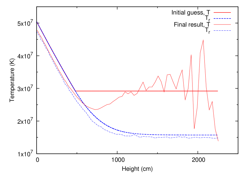
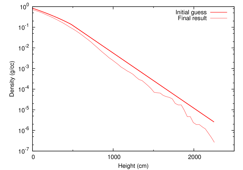
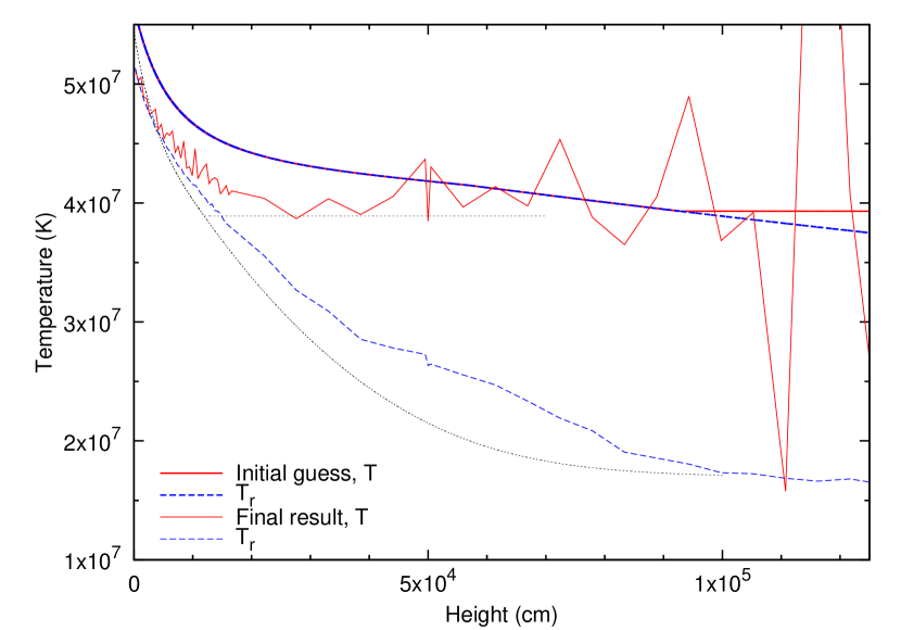
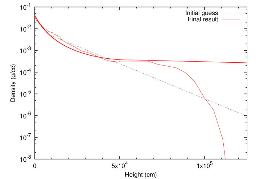
Figure 1.— Initial guess for the material and radiation temperature (the curves labeled “$T$” and “$T_{r}$”, respectively; left panels) and the density (right panels) as a function of the radial distance above the atmosphere base $r-r_{\rm base}$, for atmosphere models with solar composition, surface gravity $g_{\rm base}=10^{14}~{}{\rm cm~{}s^{-2}}$, and luminosity ratio $l_{\rm proj}=0.8$ (top panels) or $l_{\rm proj}=1.09$ (bottom panels). The temperature and density profiles at the end of the calculation are also shown (“Final result”; cf. Section 5). The $l_{\rm proj}=0.8$ profiles were generated using the “thin” atmosphere approximation while the $l_{\rm proj}=1.09$ profiles were generated using the “extended” atmosphere approximation (see text); in the bottom panels the $l_{\rm proj}=1.08$ profiles are shown for comparison as black/dotted lines.

For the initial guess above, if $F\geq F_{\rm crit}$ for certain regions in the atmosphere (see Section 2.3), we switch to an “extended” atmosphere approximation for those regions. To obtain an initial guess for extended regions, we assume that the flux remains at the critical level

$$F=F_{\rm crit}$$ (72)

throughout the region (Paczynski & Anderson, 1986). In steady state and radiative equilibrium (where the material emits as much radiation as it absorbs), we have from Equation (33) that

$$\frac{\partial\left(r^{2}F{\cal R}^{2}\right)}{\partial r}=0$$ (73)

or that

$$F=\frac{L_{\rm proj}}{4\pi r^{2}}\left(\frac{{\cal R}_{\rm base}}{{\cal R}}\right)^{2}$$ (74)

[cf. Equation (55)]. As in the thin-atmosphere case, in steady state with $P_{rr}=u/3$, isotropic $\kappa_{\nu}^{\rm tot}$ and $j_{\nu}^{\rm tot}$, and $u+P_{rr}\ll\rho c^{2}$, we have from Equations (38) and (72) that

$$\frac{1}{3}\frac{\partial u}{{\cal V}\partial r}\equiv=\frac{4a}{3}\frac{\partial T_{r}}{{\cal V}\partial r}=-\rho g_{r}\,.$$ (75)

We use the above assumptions, Equation (63) as an approximation for $\kappa_{F}^{\rm tot}$, and $T=T_{r}$ [cf. Equation (68)], along with Equations (72) and (74), to solve for $T_{r}$ and $T$ as functions of $r$; and then Equation (75) to solve for $\rho$ as a function of $r$. Note that Equations (72) and (74) combined give

$$\kappa_{F}^{\rm tot}=\frac{4\pi cGM}{L_{\rm proj}}{\cal V}\left(\frac{{\cal R}}{{\cal R}_{\rm base}}\right)^{2}\propto\frac{1}{1+z}\,;$$ (76)

that is, $\kappa_{F}^{\rm tot}$ must decrease toward the base of the atmosphere, since the redshift factor $1+z$ is largest there. This scaling is possible because the total scattering cross section drops toward the inner, hotter part of the atmosphere according to Equation (63). Solving Equation (76) for $T$ yields temperature profiles similar in shape to those in figure 1 of Paczynski & Anderson (1986). In the very outer layers of the atmosphere, if $T$ found in this manner is less than $T$ given by Equation (68), we revert to the “thin” atmosphere method outlined earlier [but with $F$ given by Equation (74) now]. Example initial guesses are given in Figure 1 for both a thin atmosphere and an atmosphere with an extended region. As can be seen in the figure, our initial guesses tend to overestimate the end-of-calculation temperatures and densities. This is particularly true for extended atmospheres, where the flux at any point in the atmosphere is close to the critical value such that small changes in $l_{\rm proj}$ lead to large changes in the temperature and density profiles. For example, in the solar, $g_{\rm base}=10^{14}~{}{\rm cm~{}s^{-2}}$, $l_{\rm proj}=1.09$ model our $l_{\rm proj}=1.08$ initial guess is a much better fit to the results of Section 5 (differing in $T_{r}$ by $<10\%$ in most places) than our $l_{\rm proj}=1.09$ initial guess (differing in $T_{r}$ by $>20\%$ in most places).

3.3. Monte Carlo method

The radiation transfer and material energy equations are solved using an implicit Monte Carlo (IMC) method; we discuss the basics of the method here but refer to the original paper (Fleck & Cummings 1971; see also Wollaber 2008) for details. We also discuss here how we implement general relativistic effects within the method. In the Appendix we discuss our Compton scattering algorithm and our treatment of stimulated scattering.

The material quantities are defined on a one-dimensional grid of cells and change at the end of each time step, as discussed above; but the radiation field is represented by discrete, stochastic particles that evolve continuously in space and time and can travel in any direction. Each Monte Carlo particle represents a packet of photons that are emitted at approximately the same radius and time, and are all moving in approximately the same direction with approximately the same frequency. Note that we do not localize these packets in polar angle or azimuthal angle; instead, we exploit the spherical symmetry of the model by grouping all similar photons across the entire $4\pi$ steradians of (spatial) solid angle into one “packet”. Therefore, we do not track location angles for the particles (only direction angles; see below).

Because the material quantities are only updated at the end of the time step but the radiation field evolves continuously in time, beginning-of-time-step values for, e.g., the material temperature are used during radiation-matter interactions (photon emission, absorption, and scattering). Solving Equation (5) as it is written, i.e., explicitly, can lead to large fluctuations in the radiation and material energies. The solution proposed by Fleck & Cummings (1971) is to treat the radiation transfer equation (Section 2.1) in a more implicit manner, by using the end-of-time-step material temperature $T^{n+1}$ for $B_{\nu}(T)$ in the equation, rewriting the equation in terms of the beginning-of-time-step temperature value, and then solving the resulting equation using Monte Carlo techniques. The expression for $T^{n+1}$ is found from the material energy equation (Section 2.2) assuming $I_{\nu}$ is given by its current value (not its average value over the time step) and that scattering is isotropic. Following their method, we obtain a new version of Equation (5) that differs only in the $j_{\nu}^{\rm tot}$ term [cf. Equation (3)], now given by

$$j_{\nu}^{\rm tot}=f_{\rm abs}j_{\nu}+(1-f_{\rm abs})j_{\nu}^{\rm eff}+j_{\nu}^{\rm sc}(\hat{\Omega})\,,$$ (77)

where

$$j_{\nu}^{\rm eff}=\chi_{\nu}\rho\int_{0}^{\infty}d\nu^{\prime}\kappa_{\nu^{\prime}}\int_{4\pi}d\Omega^{\prime}I_{\nu^{\prime}}(\hat{\Omega})$$ (78)

is the effective scattering coefficient,

$$\chi_{\nu}=\frac{\kappa_{\nu}B_{\nu}(T)}{\int_{0}^{\infty}d\nu^{\prime}\kappa_{\nu^{\prime}}B_{\nu^{\prime}}(T)}$$ (79)

is the reemission spectrum,

$$f_{\rm abs}=\frac{1}{1+(4aT^{3}/\rho c_{V})c\Delta t_{\rm cell}\rho\kappa_{\rm P}}$$ (80)

is the effective absorption factor and

$$\kappa_{\rm P}=\frac{\int_{0}^{\infty}d\nu\kappa_{\nu}B_{\nu}(T)}{\int_{0}^{\infty}d\nu B_{\nu}(T)}$$ (81)

is the Planck-averaged absorption opacity. In the IMC method, a fraction $f_{\rm abs}$ of the total emission in a time step is handled in the standard way, by creating new particles and decreasing the cell energy (see below); but the remaining $1-f_{\rm abs}$ is handled through “effective scattering”: a particle undergoing effective scattering is given a new direction, uniformly random, and a new frequency, random but weighted by $\chi_{\nu}$. Physically, the material absorbs the particle and then shortly after reemits the absorbed energy isotropically. Numerically, the time step is too large for the absorption and emission processes to be resolved separately, such that they appear as one scattering process ($f_{\rm abs}\rightarrow 0$ as $\Delta t_{\rm cell}\rightarrow\infty$).

The simulation is initially populated with Monte Carlo particles according to Equation (66). During each time step, the code creates new Monte Carlo particles to simulate the process of emission. The number of particles created depends on how many particles are already in the simulation: if there are relatively few existing particles then many are created, but if the number of existing particles is close to the maximum allowed value then few are created. We typically set the maximum to $10^{6}$ particles; we want enough particles to populate every cell and frequency group (Section 3.1), but not so many that our simulation runs slowly. For each particle, the details of its creation (location, direction, etc.) are randomly chosen. The cell of creation is randomly chosen with weighting $\Delta U_{\rm cell}$, the amount of energy the cell emits in the time step. Using Equations (10), (33), and (77) we have

$$\Delta U_{\rm cell}=f_{\rm abs}c\Delta t_{\rm cell}V_{\rm cell}\rho\kappa_{\rm P}aT^{4}\,,$$ (82)

where $V_{\rm cell}$ is the volume of the cell and $\Delta t_{\rm cell}$ is the time step for the cell (see below). For simplicity, the radius within the cell and the time within the time step are randomly chosen with uniform weighting; from Equation (10), the direction is weighted uniformly (isotropically) while the frequency is weighted by $\kappa_{\nu}B_{\nu}(T)$. The particle also has an energy weight, equal to the total energy of the photon packet. This is not randomly chosen; instead, all of the particles “emitted” in a time step have the same energy weight, given by

$$w_{\rm emit}=\frac{\sum_{\rm cells}\Delta U_{\rm cell}}{N_{\rm emit}}$$ (83)

with $N_{\rm emit}$ the number of Monte Carlo particles emitted in that step. At the end of the time step the cell temperature is adjusted due to emission using

$$\Delta T_{\rm emit}=-\frac{\Delta U_{\rm cell}}{V_{\rm cell}\rho c_{V}}$$ (84)

(see below).

Particles are also created at the inner boundary of the simulation, the base of the atmosphere. Here the physical process for the creation of the particles is not emission, but the escape of photons from the hot layers beneath the atmosphere. As before, the details of creation are chosen randomly; the time within the time step is chosen with uniform weighting, while from Equation (35), the direction is weighted by $\mu$ and the frequency is weighted by $B_{\nu}$. The energy weight for these particles is

$$w_{\rm base}=\frac{\Delta U_{\rm base}}{N_{\rm base}}$$ (85)

with $N_{\rm base}$ the number of particles created at the base in the time step and $\Delta U_{\rm base}$ the energy entering the simulation from the base of the atmosphere. From Equations (35) and (53) we have

$$\Delta U_{\rm base}=\Delta t_{\rm base}A_{\rm base}\sigma_{\rm SB}T_{\rm base}^{4}\,,$$ (86)

where $A_{\rm base}$ is the area of the base and $\Delta t_{\rm cell}$ is the time step at the base [cf. Equation (67)].

The created particles (photon packets) are transported according to the left-hand side of Equation (5). If general relativistic effects are ignored, the particles travel in straight lines. For a particle traveling a distance $s$ from the position $(r_{\rm old},\theta_{\rm old},\phi_{\rm old})$ and moving in the direction $\hat{\Omega}$ initially defined by $\hat{\Omega}=\Omega_{r,\rm old}\hat{r}_{\rm old}+\Omega_{\theta,\rm old}\hat{\theta}_{\rm old}$, where $\Omega_{r,\rm old}\equiv\mu_{\rm old}$, the new radius of the particle is given by the law of cosines:

$$r_{\rm new}=\sqrt{s^{2}+r_{\rm old}^{2}+2sr_{\rm old}\mu_{\rm old}}\,.$$ (87)

The new polar angle for the direction could be found in a similar manner, using Equation (87) and the law of cosines for $r_{\rm old}$ in terms of $s$ and $r_{\rm new}$: $\mu_{\rm new}=(s+r_{\rm old}\mu_{\rm old})/r_{\rm new}$. However, in our code this quantity is solved in a manner that is more consistent with general relativity, as we describe below. Note that because of the spherical symmetry of the problem, we orient the direction $\hat{\Omega}$ such that it has no azimuthal component $\Omega_{\phi}$ and do not track the azimuthal angle for the position (or the polar angle for the position, once $\mu_{\rm new}$ is known).

After the particle is transported using Equation (87), we apply general relativistic effects. Due to the gravitational redshift term in Equation (5) [the one proportional to $(g_{r}/c^{2})(\partial(I_{\nu}\nu^{-3})/\partial\nu)$], the new frequency and weight of the particle are given by

$$\nu_{\rm new}=\nu_{\rm old}\frac{{\cal R}_{\rm old}}{{\cal R}_{\rm new}}$$ (88)

and

$$w_{\rm new}=w_{\rm old}\frac{{\cal R}_{\rm old}}{{\cal R}_{\rm new}}\,;$$ (89)

the number of photons in the packet remains the same but their energy changes. Time dilation [represented by the $(1/c)(\partial u/{\cal R}\partial t)$ term in Equation (5)] is taken into account by using a different

$$\Delta t_{\rm cell}=\Delta t_{\rm base}\frac{{\cal R}}{{\cal R}_{\rm base}}$$ (90)

for each cell. For simplicity we consider gravitational light bending [represented by the $(g_{r}/c^{2})(\partial I_{\nu}/\partial\mu)$ term] as a perturbation on the particle trajectory; see Section 4.6. The trajectory of a photon traveling in a Schwarzschild geometry is given by (e.g., Misner et al., 1973)

$$\frac{d\theta}{dr}=-\frac{b}{r\sqrt{r^{2}-b^{2}\left(1-2GM/c^{2}r\right)}}\,,$$ (91)

where $b$ is the impact parameter. The impact parameter can be found by using the pre-transport position and direction quantities ($r_{\rm old}$, $\Omega_{r,\rm old}$, and $\Omega_{\theta,\rm old}$) to equate Equation (91) and

$$\frac{d\theta}{dr}=-\frac{\Omega_{\theta}}{r\Omega_{r}}\,,$$ (92)

which describes the local propagation direction of the particle. If $\hat{\Omega}=\pm\hat{\theta}$ [such that $\Omega_{r}=0$ and Equation (92) is undefined], we set $b=\pm r_{\rm old}/\sqrt{1-2GM/c^{2}r_{\rm old}}$. We then solve for $\mu_{\rm new}\equiv\Omega_{r,\rm new}$ by equating Equations (91) and (92) with $r_{\rm new}$ from Equation (87). Our approximation of using the Newtonian $r_{\rm new}$ rather than a post-transport radius calculated self-consistently with Equation (91) is accurate to first order in $(2GM/c^{2}r)(\Delta r/r)$ (Section 4.6).

After the particle is transported and general relativistic effects are applied, it undergoes an event. There are five particle events that our code accounts for: 1) the particle is absorbed; 2) the particle is effectively scattered (see earlier in this section); 3) the particle is actually scattered; 4) the particle reaches the boundary of a cell; 5) the time step ends. Each of these events has a distance associated with it, e.g., for event 4, the distance the particle needs to travel to reach the boundary of the cell. For each particle, the code determines which of the events has the shortest distance (i.e., which event will happen first), transports the particle by that distance [$s$ in Equation (87)], and then carries out the event as described below.

For event 1: absorption and event 2: effective scattering, the distance traveled is given by

$$s_{\rm abs}=-\frac{\ln\xi}{\rho\kappa_{\nu}}\,,$$ (93)

where $\xi$ is a (uniformly distributed) random number between 0 and 1. Equation (93) comes from assuming a probability for photon absorption of $e^{-\rho\kappa_{\nu}s}$ (Fleck & Cummings, 1971). A fraction $f_{\rm abs}$ of the particles undergo absorption, in which case the location of the event and the energy weight of the particle are recorded and then the particle is destroyed; the remainder undergo effective scattering, in which case the direction and frequency are adjusted as described earlier in this section and the energy weight remains at $w_{\rm new}$. For both events, the change in the radial momentum of the particle is recorded using only the pre-scattering contribution:

$$\Delta p_{r,\rm abs}=-\frac{\mu_{\rm new}w_{\rm new}}{c}\,;$$ (94)

we do not include the post-scattering contribution $\mu^{\prime}_{\rm new}w_{\rm new}/c$ in $\Delta p_{\rm abs}$ here, since due to the isotropic nature of effective scattering this contribution is on average zero (we do not record the momentum of emitted particles either, for the same reason). For event 3: actual scattering, the distance traveled is given by Equation (93) but with $\kappa_{\nu}^{\rm sc}$ in place of $\kappa_{\nu}$. The direction and frequency of the particle are adjusted based on the (Compton) scattering opacity in Equation (31), as described in the Appendix (cf. Canfield et al., 1987), the energy weight is adjusted according to

$$w^{\prime}_{\rm new}=\frac{\nu^{\prime}_{\rm new}}{\nu_{\rm new}}w_{\rm new}\,,$$ (95)

and then the location and change in energy weight is recorded. The change in momentum is recorded using

$$\Delta p_{r,\rm sc}=\frac{\mu^{\prime}_{\rm new}w^{\prime}_{\rm new}-\mu_{\rm new}w_{\rm new}}{c}\,.$$ (96)

For event 4: cell boundary, the distance traveled depends on the particle direction. The first cell boundary reached will be the inside boundary $r_{\rm in}$ if (using the Pythagorean theorem)

$$r_{\rm old}\mu_{\rm old}\leq-\sqrt{r_{\rm old}^{2}-r_{\rm in}^{2}}\,,$$ (97)

otherwise it will be the the outside boundary $r_{\rm out}$. Then the distance traveled is given by the law of cosines (ignoring light bending; see above):

$$s_{\rm bnd}=\left\{\begin{array}[]{ll}-r_{\rm old}\mu_{\rm old}+\sqrt{r_{\rm old}^{2}\mu_{\rm old}^{2}+r_{\rm out}^{2}-r_{\rm old}^{2}}\,,&\rm{outside};\\ -r_{\rm old}\mu_{\rm old}-\sqrt{r_{\rm old}^{2}\mu_{\rm old}^{2}+r_{\rm in}^{2}-r_{\rm old}^{2}}\,,&\rm{inside}.\end{array}\right.$$ (98)

If the particle leaves the simulation through the inner boundary it is destroyed. If the particle leaves the simulation through the outer boundary, its energy weight is recorded and then the particle is destroyed. For event 5: end of time step, the distance traveled is given by the speed of light multiplied by the time remaining until the end of the time step. After the particle is propagated to event 5, its properties (location, direction, frequency, and energy weight) are stored in memory until the next time step.

After the event, if the particle has not escaped the simulation or been absorbed and there is still time remaining in the current time step, the process continues with another event. At the end of the time step, the energy in each cell is decreased by the combined energy weights of all particles created in the cell during the step (through emission; see above), increased by the energy weights of all particles destroyed in the cell during the step (through absorption), and modified by all energy weight changes (due to scattering); cf. Equation (84). The fluence (the time- and area-integrated flux) at the outer boundary of the simulation ${\cal F}_{\rm surf}$ is increased by the quantity $w/c$ for all particles that cross the boundary, while the group-dependent fluence ${\cal F}_{\rm g,surf}$ is increased by $w/c$ only for those particles with frequencies in the range of the group. Here

$${\cal F}_{\rm surf}=\sum_{\rm groups}{\cal F}_{\rm g,surf}$$ (99)

and

$${\cal F}_{\nu,\rm surf}\simeq{\cal F}_{\rm g,surf}/\Delta\nu_{\rm g}\,,$$ (100)

where ${\rm g}$ is the frequency group and $\Delta\nu_{\rm g}$ is the width of that frequency group. The outgoing spectral flux at the surface $F_{\nu,\rm surf}$ and the luminosity are given by

$$F_{\nu,\rm surf}=\frac{\Delta{\cal F}_{\rm g,surf}/\Delta\nu_{\rm g}}{A_{\rm surf}\Delta t_{\cal F}}$$ (101)

and

$$L_{\rm surf}=\frac{\Delta{\cal F}_{\rm surf}}{\Delta t_{\cal F}}\,.$$ (102)

Here $\Delta t_{\cal F}$ is the time interval over which $\Delta{\cal F}_{\rm surf}$ is taken; to reduce noise, we typically use $\Delta t_{\cal F}=10^{-6}~{}{\rm s}\simeq 1000\Delta t_{\rm surf}$. Note that in the Monte Carlo method, the flux measured by counting particles crossing a cell boundary is naturally the flux in the direction normal to the boundary; there is no need to multiply each particle’s energy weight by $\mu$ [cf. Equation (35)]. This is because each particle implicitly carries with it a solid angle $\Delta\Omega$, such that when the particle intersects the boundary the energy weight is spread out over an area proportional to $\mu$.

3.4. Method for ensuring hydrostatic balance

Figure 2.— The quantity $\Delta p_{r,\rm cell}/\rho V_{\rm cell}\Delta t_{p}$ (where $\Delta p_{r,\rm cell}$ is the momentum deposited into the material; see text) as a function of height above the base of the atmosphere, for atmosphere models with solar composition, $g_{\rm base}=10^{14}~{}{\rm cm~{}s^{-2}}$, and a variety of luminosity ratios.

Every several time steps we adjust the structure of the atmosphere to maintain hydrostatic balance. We keep $\rho_{\rm base}$ fixed and adjust the mass density in the cells, attempting to satisfy Equation (46) in every cell. For stability reasons, we typically choose an interval between adjustments of $5\times 10^{-6}~{}{\rm s}\simeq 5000$ time steps, such that the atmosphere is close to radiative equilibrium, and restrict the density change in any particular cell to ten percent or less in each adjustment. The radiation term in Equation (46) is given by

$$-\frac{1}{c}\int_{0}^{\infty}d\nu\int_{4\pi}d\Omega\mu\left[-\rho\kappa_{\nu}^{\rm tot}(\hat{\Omega})I_{\nu}(\hat{\Omega})+j_{\nu}^{\rm tot}(\hat{\Omega})\right]$$

$$\qquad\qquad\qquad\qquad=\frac{\Delta p_{r,\rm cell}}{V_{\rm cell}\Delta t_{p}}\,,$$ (103)

where $\Delta t_{p}$ is the time interval over which $\Delta p_{r,\rm cell}$ is taken. To reduce noise, we typically use $\Delta t_{p}=5000\Delta t_{\rm cell}$; i.e., the momentum is differenced over the entire interval between density adjustments. Note that because of the symmetry of the model, in Equation (103) we ignore contributions to the radiation term due to momentum changes in non-radial directions. Figure 2 shows the “radiation pressure acceleration” (cf. equation 7 of Suleimanov et al., 2011b), given by the quantity $\Delta p_{r,\rm cell}/\rho V_{\rm cell}\Delta t_{p}$ from Equation (103), which should be less than or equal to $g_{r}$ when the atmosphere is in hydrostatic balance.

3.5. Reaching the end-of-calculation equilibrium

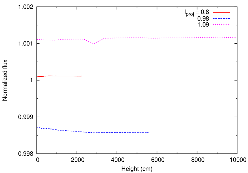
Figure 3.— The quantity $4\pi r^{2}F{\cal R}^{2}/(l_{\rm proj}L_{\rm Th}{\cal R}_{\rm base}^{2})$ (see text) as a function of height above the base of the atmosphere, for the same atmosphere models as in Figure 2.

We continue the process described in Sections 3.3 and 3.4, i.e., every time step transporting the photons and coupling them to the material in a manner described by Equations (5) and (41), and then every several time steps partially restoring hydrostatic balance using Equation (46), until steady state and radiative equilibrium is reached. Our criterion for reaching steady state is that the luminosity $L_{\rm proj}$ changes by less than one part in $10^{6}$ per time step. This criterion is typically satisfied after around $10^{6}$ time steps for thin atmospheres, more for thick atmospheres or when the system is far from hydrostatic balance. We do not explicitly check whether radiative equilibrium is reached; however, once the luminosity meets the above criterion, the quantity $r^{2}F{\cal R}^{2}$ usually varies by no more than 1% across the entire atmosphere [cf. Equation (73)]. We then adjust $T_{\rm base}$ as described in Section 3.1, and repeat the process to reach a new steady state/radiative equilibrium. We let the simulation run until the projected luminosity is within 0.2% of the desired value $l_{\rm proj}L_{\rm Th}$. At this point the simulation is very nearly in radiative equilibrium, as is shown in Figure 3.

4. Effect of various physical processes on the observed spectra

The pieces of physics we include in our simulations have varying degrees of effect on our results. Here we describe each piece.

4.1. Radiation transport

In the outer layers of a hot neutron star ($\rho\alt 1~{}{\rm g~{}cm^{-3}}$, $T\agt 10^{7}$ K), radiation transport is the dominant form of energy transport; heat conduction and convection contribute very little (Joss, 1977; Rajagopal & Romani, 1996; Potekhin et al., 1997; Weinberg et al., 2006). We therefore only consider radiation transport in our calculations here. Since we are modeling the deviation of the outgoing radiation spectra from a Planck function (i.e., from blackbody radiation), our problem is inherently multi-frequency. We assume a spherically symmetric atmosphere and a spherically symmetric but anisotropic radiation field (see Section 3). Axially symmetric or fully three-dimensional atmospheres are more accurate if the neutron star is highly non-spherical (due to rotation) or the thermonuclear burning powering the burst is not uniform over the star (see Miller 2013 and references therein), but they are computationally very expensive.

An anisotropic radiation field is necessary to correctly model the optically thin, outer atmosphere (e.g., Rybicki & Lightman, 1986). For example, we find that the radiation energy density in the outer layers is typically a few percent lower when using anisotropic radiation transport than when using radiation diffusion. Note that while the Monte Carlo method has many advantages, including the automatic treatment of multi-frequency and anisotropic physics mentioned above, one key disadvantage is stochastic noise. The effect of this noise can be seen in many of the figures in this paper; it is most noticeable at the high-$r$ end of the material temperature profiles (e.g., Figure 1) and at the high- and low-frequency ends of the spectra (e.g., Figure 5), where there are fewer particles. We have run our simulations with enough particles to compensate for this noise, but the computation time is an order of magnitude longer than for a diffusion calculation with a converged spectrum.

4.2. Radiation-material interaction

For a review on interactions between radiation and material, see Castor (2004). We assume that the radiation at the base of the atmosphere is in thermal equilibrium with the material there. For this to be an accurate assumption, most photons emitted at the base of the atmosphere must be absorbed before they escape; this latter condition occurs when (Rybicki & Lightman, 1986)

$$\sqrt{\tau_{\nu,\rm base}\tau_{\nu,\rm base}^{\rm tot}}\agt 1\,,$$ (104)

where $\tau_{\nu,\rm base}$ is the absorption-only optical depth at the base of the atmosphere and $\tau_{\nu,\rm base}^{\rm tot}$ is the total (absorption plus scattering) optical depth [cf. Equation (71)]. For the highest frequencies of interest here ($h\nu\sim 30$ keV; cf. Suleimanov et al., 2011b), the absorption opacities are very small, such that satisfying Equation (104) requires frequency-averaged total optical depths $\tau_{\rm base}^{\rm tot}\agt 100$. Ideally we should place the atmosphere base deep enough that $\tau_{\rm base}^{\rm tot}\gg 100$, for greater accuracy; for Monte Carlo calculations, however, the computation time increases quadratically with total optical depth (Densmore et al., 2007) and so we place the base right at this critical value. We have performed convergence studies in $\tau_{\rm base}^{\rm tot}$ for a few cases and found differences of only a couple percent between the spectra in the $\tau_{\rm base}^{\rm tot}=100$ case and the converged answer, and no detectable difference between the color correction factors for the two cases.

A change to the radiation field in the optically thick, inner layers of the atmosphere diffuses outward at a velocity $v_{\rm diff}\simeq c/\tau^{\rm tot}$, such that it reaches the surface after a time $t_{\rm diff}\simeq H\tau^{\rm tot}/c$, where $H$ is the thickness of the atmosphere; for $\tau_{\rm base}^{\rm tot}=100$ we have that thin atmospheres reach radiative equilibrium in $\sim 10^{-5}$ s, while extended ($\sim 10$ km) atmospheres reach radiative equilibrium in $\sim 10^{-2}$ s. For comparison, the temperature at the base of the atmosphere, which tracks the X-ray burst evolution, changes on a time scale of several seconds (the burst time). We therefore treat the temperature at the base of the atmosphere as constant over our simulation time and evolve the system to steady state (cf. Shaposhnikov & Titarchuk, 2002).

We consider both scattering and absorption-emission of photons by electrons. Specifically, we include Compton scattering – scattering of photons by free electrons (or “nearly free” electrons; see Section 4.3); inverse bremsstrahlung – absorption of photons by free electrons in the presence of an ion – and photoionization/photoexcitation – bound-free/bound-bound transitions of electrons through absorption of photons; and the reverse processes (that is, emission of photons by free or bound electrons). The exact implementation of each of these radiation-material interactions is discussed in Section 4.3.

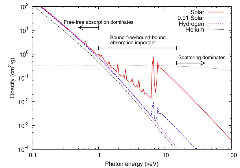
Figure 4.— Absorption opacity as a function of photon energy, for $\rho=0.46$ ${\mathrm{cm}}^{2}$ ${\mathrm{g}}^{-1}$and $k_{\rm B}T=1$ keV. The opacities shown here are averaged over frequency group; in our simulation we use 300 logarithmically spaced groups in the the range $\nu=10$ eV to $1$ MeV (see text). Each model curve is labeled with the atmosphere composition for that model. For the “Solar” composition model, the scattering opacity ignoring stimulated scattering [cf. Equation (13)] is also shown for comparison, as a thin solid line. The arrows show the approximate frequency regions where each type of absorption or scattering is important for these models.

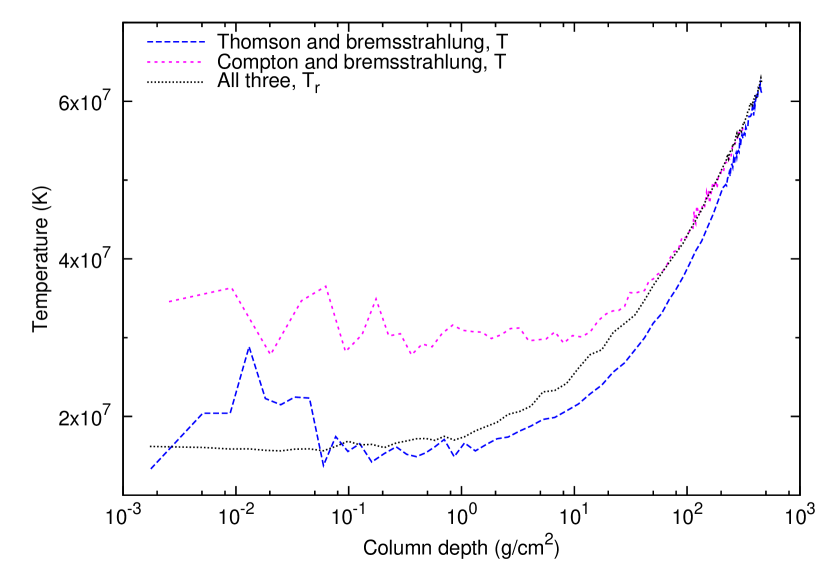
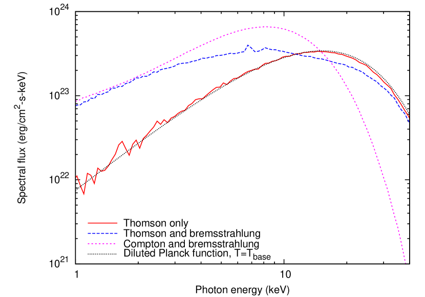
Figure 5.— Material and radiation temperature profiles (top panel) and the outgoing radiation spectrum (bottom panel), for a solar-composition, $g_{\rm base}=10^{14}~{}{\rm cm~{}s^{-2}}$, $l_{\rm proj}=0.98$ atmosphere. The three line colors/patterns represent three different models for scattering and absorption: red/solid curves represent Thomson scattering only, blue/long-dashed curves represent Thomson scattering and bremsstrahlung, and purple/short-dashed curves represent Compton scattering and bremsstrahlung. In the top panel, we do not show a curve of the material temperature $T$ for the model with Thomson scattering only, since the material has no effect on the outgoing spectrum in this case. In addition, we only show one representative curve of the radiation temperature $T_{r}$ (as a black/dotted line), since the $T_{r}$ curves are very similar for all three models. In the bottom panel, we show for comparison the diluted Planck function $\epsilon B_{\nu}(T_{\rm base})$ with $\epsilon=F/\sigma_{\rm SB}T_{\rm base}^{4}$ (see text).

Figure 4 shows the contributions of the scattering and absorption processes to the total frequency-dependent opacity. Inverse bremsstrahlung is the main contributor to the total opacity at low frequencies, because of the $\nu^{-3}$ dependence of this process. Compton scattering dominates at higher frequencies, except at low densities and temperatures for solar-like compositions, where photoionization and photoexcitation dominate the $h\nu\sim 1$–$10$ keV range. In terms of the outgoing radiation spectra, photoionization and photoexcitation cause absorption lines and edges for metal-rich bursts at low luminosities ($l_{\rm proj}\alt 0.01$, see Figure 12), but have little effect at high luminosities. Bremsstrahlung/inverse bremsstrahlung and Compton scattering, on the other hand, have strong effects at all compositions and luminosities we consider in this paper. Compton scattering is also the main contributor to the optical depth in the atmosphere, and therefore sets the general structure of the radiation there. To highlight the effects of these latter two processes we compare here three atmosphere models, shown in Figure 5: one with Thomson scattering (the non-relativistic limit of Compton scattering) only, one with Thomson scattering and bremsstrahlung, and one with Compton scattering and bremsstrahlung (cf. Madej et al., 2004; Miller et al., 2011). The top panel of Figure 5 shows the material and radiation temperatures $T$ and $T_{r}$ as a function of column depth for each model, while the bottom panel shows the outgoing spectrum.

In the Thomson-scattering-only atmosphere, the radiation field near the surface differs in magnitude from that at the base, but has the same frequency distribution; i.e., the radiation field is represented by a Planck function at the base [$I_{\nu}(\hat{\Omega})=B_{\nu}(T_{\rm base})$] and a diluted Planck function at the surface [$I_{\nu}(\hat{\Omega})=\epsilon(\hat{\Omega})B_{\nu}(T_{\rm base})$, where $\epsilon(\hat{\Omega})$ is the frequency-independent dilution factor]. This is because, although Thomson scattering reduces the number of photons traveling outward from the base, the direction and amount of scatter are independent of frequency and no energy is transferred between the photons and the material. For this type of atmosphere the material and the radiation are decoupled; i.e., $T$ and $T_{r}$ are independent of each other.

In the bremsstrahlung-plus-Thomson atmosphere, due to the strong frequency dependence of the bremsstrahlung process, low-frequency photons are absorbed after traveling only a short distance, and those that reach the surface are emitted from nearby, relatively cool layers. Hence, in this atmosphere the radiation field at low frequencies is described by (when the material is in LTE) $I_{\nu}=B_{\nu}(T)$, where $T$ is the local material temperature. Mid-frequency photons are emitted from deeper, hotter layers, and are described by $I_{\nu}=B_{\nu}(T_{\nu}^{*})>B_{\nu}(T)$ with $T_{\nu}^{*}>T$ that increases with frequency. The highest-frequency photons are neither absorbed nor emitted, but are scattered up from the base; the radiation field at these frequencies is $B_{\nu}(T_{b})/A\gg B_{\nu}(T)$, where $T_{b}$ is the temperature at the base of the atmosphere and $A$ is a normalization constant. The total radiation energy density is therefore larger than $(1/c)\int d\nu\int d\Omega B_{\nu}(T)=aT^{4}$, such that $T_{r}>T$ (cf. Mihalas, 1978). The effect is strongest in the outer layers, where the radiation is farthest from thermal equilibrium. At the surface and in steady state, $T\sim 0.5T_{r}$ for this type of atmosphere.

Compton scattering modifies this picture by transferring energy between the radiation field and the material with each scatter. During a scattering event, the fraction of energy gained by the photon is

$$\frac{\Delta\nu}{\nu}=\frac{4k_{\rm B}T-h\nu}{m_{e}c^{2}}\,,$$ (105)

assuming the electrons in the material are in thermal equilibrium (Rybicki & Lightman, 1986). Low-to-mid-frequency photons gain a small amount of energy per scatter ($\Delta\nu\sim\pm 0.01\nu$), and scatter at most a few times before they are absorbed, such that $I_{\nu}\simeq B_{\nu}(T)$ or $B_{\nu}(T_{\nu}^{*})$ as above; here, however, the deeper layers are not necessarily hotter than the local layer. High-frequency photons lose a large amount of energy per scatter ($\Delta\nu\sim 0.1\nu$) and scatter multiple times, such that the radiation field at high frequencies is of much lower energy density than in the Thomson-scattering case. The material temperature $T$ is therefore larger relative to $T_{r}$ in this type of atmosphere, and in the outer layers where the absorption opacity is lowest, the downscatter effect is so strong that $T>T_{r}$.

Note that in radiative equilibrium, where the flux through the atmosphere is constant, the radiation temperature $T_{r}$ decreases with increasing radius at a prescribed rate; e.g., in the diffusion approximation, $F\equiv-(c/\rho\kappa^{\rm tot})d(aT_{r}^{4})/dr={\rm constant}$. The material temperature $T$ has very little effect on this rate because it only enters the flux equation through the opacity, and only very weakly in the scattering-dominated atmospheres considered here. This is why the models shown in Figure 5, which all have the same atmospheric flux, have nearly the same $T_{r}$ profiles. Because the $T_{r}$ profile is essentially fixed by the flux $F$ (or $l_{\rm proj}$ in our formalism; see Section 3.1), the $T$ profile adjusts to the $T_{r}$ profile, not the other way around. In the bremsstrahlung-plus-Thomson atmosphere $T$ drops faster than $T_{r}$ starting at an optical depth of of unity, and continues to separate from $T_{r}$ until $T$ is half $T_{r}$ at the surface. In contrast, in the bremsstrahlung-plus-Compton atmosphere $T$ drops faster than $T_{r}$ in the mid layers of the atmosphere, but then rises in the outer layers to be equal to or greater than $T_{r}$ (in addition to Figure 5, see, e.g., figure 3 of either Madej et al. 2004 or Suleimanov et al. 2012). Effectively, scattering transports many high-frequency photons to the outer layers and these photons can not be efficiently absorbed by inverse bremsstrahlung (due to its $\nu^{-3}$ dependence), so the layers cool off. At the same time, however, many of these high-frequency photons are downscattered, causing the outer layers to heat up. The balance between these two attributes of scattering determines the overall temperature structure in the atmosphere.

4.3. Opacity

Our absorption opacities are provided by the LANL TOPS code, which calculates frequency-averaged opacities from the monochromatic cross sections in the LANL OPLIB database (Magee et al., 1995; Frey et al., 2013). Specifically, we request that the TOPS code average opacities over each frequency group using a Planck (linear with weight $B_{\nu}$) average at the local material temperature $T$. We have chosen this averaging for simplicity, since the online version of TOPS provides the absorption opacity in terms of a Planck average and since using $T$ requires fewer variables in the lookup table (only $\rho$ and $T$ rather than $\rho$, $T$, and $T_{r}$). We have checked for a few cases that using $T_{r}$ or a Rosseland (inverse with weight $\partial B_{\nu}/\partial T$) average instead does not noticeably change our results; but we do not expect it to due to the narrow widths of the frequency groups in our simulations. Note that we can not use a mixture of Rosseland and Planck averages as in Frey et al. (2013), because we are using Monte Carlo transport where there is no distinction between the opacity used in modeling the transport of photons and that used in the equilibration of the photons and the material.

The OPLIB database takes into account the ionization level of the material, though the atmosphere is mostly ionized at the temperatures considered here. A plasma cutoff is included in the form of an artificially large opacity for $h\nu\alt 30\rho^{1/2}$ eV, though this cutoff is lower than the lowest frequencies of interest in our simulations except in the deepest parts of the atmosphere for the hottest stars. The correction factor for stimulated emission, $1-e^{-h\nu/k_{\rm B}T}$ [Equation (11)], is automatically included in the opacities returned from the database through TOPS. Thermal broadening is also included in the database.

Figure 6.— Multigroup absorption opacity as a function of frequency group, for $\rho=10^{2}$ ${\mathrm{cm}}^{2}$ ${\mathrm{g}}^{-1}$and $k_{\rm B}T=10$ keV. Both LTE and non-LTE opacities are shown; the non-LTE opacities are generated using the RADIOM model (see text).

The monochromatic opacities contained within the OPLIB database are generated under the assumption that the material is in LTE, i.e., that the bound-electron populations and the free-electron energy distribution can be accurately described by Saha-Boltzmann statistics. By using the database we implicitly adopt this assumption in our paper; this also allows us to derive the emission coefficients from the database results, using Kirchoff’s law of thermal radiation [Equation (10)]. At the base of the XRB atmosphere the radiation-material system is in thermal equilibrium (Section 4.2). However, at optical depths of a few or less, this is no longer true: the radiation field is highly non-Planckian and $T\neq T_{r}$. Note that the material can be in LTE even when it is not in equilibrium with the radiation field (i.e., when $T\neq T_{r}$; e.g., Rybicki & Lightman, 1986; Castor, 2004). This happens when material-material collisions dominate radiation-material interactions (see Section 4.4). As is discussed in Section 4.4, in the outer layers of the atmosphere the material is not in thermal equilibrium even with itself. Assuming LTE conditions in these layers can introduce large errors in the bound-electron contributions to the frequency-dependent absorption opacities there. However, the error in the outgoing spectrum should be much less, due to two mitigating factors: first, the layers where LTE conditions break down are at low optical depths ($\tau^{\rm tot}\alt 0.1$), such that they contribute very little to the spectrum; and second, at the high temperatures and mostly hydrogen compositions of the XRB atmosphere (but see Section 4.7) bound transitions contribute only a small part of the total opacity. We did not implement non-LTE opacities in our model, so we can not compare LTE and non-LTE outgoing spectra; however, in Figure 6 we show for typical conditions in the outer layers the frequency-dependent LTE absorption opacities and their non-LTE approximations generated using the RADIOM model (see Section 4.4; Busquet, 1993). For certain frequencies the difference in the absorption opacity is a factor of two or more.

For our scattering opacity we use the Klein-Nishina differential cross section (e.g., Rybicki & Lightman, 1986), which is exact for Compton scattering of unpolarized radiation. Using the exact Klein-Nishina cross section rather than the Thomson approximation (which is $\kappa_{\nu}^{\rm sc}\simeq Y_{e}\sigma_{\rm Th}/m_{u}$) is essential for accurate modeling of high-luminosity atmospheres. In particular, since the Klein-Nishina total cross section is smaller than that of the Thomson approximation at high frequencies, we can have $l_{\rm proj}>1$, i.e., a projected luminosity greater than the Thomson Eddington luminosity of Equation (56), without mass loss. In addition, due to the drop in the Klein-Nishina cross section at high frequencies, the frequency-integrated scattering opacity decreases with increasing temperature at such a rate that $F<F_{\rm crit}$ [Equation (49)] throughout the atmosphere: even though $r^{2}F$ increases toward the base of the atmosphere due to the strong general relativistic effects there, $r^{2}F_{\rm crit}$ increases faster (see Section 3; Paczynski & Anderson, 1986; Suleimanov et al., 2012).

For $n_{e}$ in our scattering cross section formula [Equation (13)] we use the number density of all electrons, bound or free. This is because, for typical photons in the atmosphere, the energy $h\nu\agt 100$ eV is much larger than the binding energy of any bound electrons, such that the photons see all electrons as effectively free. In this regime the scattering cross section for bound electrons, like that for free electrons, is given by the Klein-Nishina form; Rayleigh scattering and other forms of bound-electron scattering can be ignored (Eisenberger & Platzman, 1970; Rybicki & Lightman, 1986).

Figure 7.— Material and radiation temperature profiles (top panel) and the outgoing radiation spectrum (bottom panel), for a solar-composition, $g_{\rm base}=10^{14}~{}{\rm cm~{}s^{-2}}$, $l_{\rm proj}=0.98$ model atmosphere with and without stimulated scattering.

To simulate repeated scatterings of photons by a distribution of electrons we solve the Boltzmann equation for Compton scattering; our method is discussed in the Appendix. Suleimanov et al. (2012) compared XRB atmosphere models solving the full Boltzmann equation with ones solving the Kompaneets approximation (see, e.g., Rybicki & Lightman, 1986), and found differences of around $5\%$ in the outgoing spectra at near-Eddington luminosities. Note that while the direct scattering terms in the Boltzmann equation are naturally handled by the Monte Carlo method, the stimulated scattering terms [$1+n_{\nu}$ and $1+n_{\nu^{\prime}}$ in Equations (13) and (32)] are not easily accounted for. In our calculations we have included an approximation to stimulated scattering, described in the Appendix. Stimulated scattering is most important at high temperatures and densities. Without it, $T\neq T_{r}$ in the deep parts of the atmosphere. In the hottest atmospheres, many high-frequency photons originate from layers where stimulated scattering is important, such that there is a noticeable change in both the outgoing spectra and the color correction factors when stimulated scattering is included in our models compared with when it is ignored. Figure 7 shows the effect of stimulated scattering on a hot atmosphere, both for the temperature profile and the outgoing spectrum.

4.4. Plasma physics

In the neutron star atmosphere, ions and free electrons collide much more frequently with each other than with photons. For example, electron-electron collision rates are around $10^{14}~{}(\rho/1~{}{\rm g~{}cm^{-3}})~{}{\rm s^{-1}}$ (e.g., Huba, 2013), while electron-photon rates are five orders of magnitude lower. We therefore assume that the ions and (free) electrons are in equilibrium with themselves and each other, i.e., that they are Maxwellian and have the same temperature $T_{i}=T_{e}$. We assume that the ions and electrons have Maxwell-Boltzmann, i.e., non-relativistic, distributions. This is an excellent assumption for the ions, since $k_{\rm B}T\ll m_{p}c^{2}$, but leads to an error of $\alt 2\%$ in the cumulative distribution for the electrons at the highest temperatures considered here. Since the XRB atmosphere temperatures are large ($\agt 1$ keV), the ions and electrons are also assumed to be ideal gases.

Note that while the free electrons, which are in equilibrium, obey Maxwell-Boltzmann statistics, the bound electrons do not necessarily. This is because the atomic level populations are set by the balance between radiative and inelastic collisions, which transfer energy to or from the electrons and cause them to transition between levels; the great majority of electron and ion collisions are elastic and do not affect this balance (e.g., Mihalas & Mihalas, 1984). Therefore, while it is appropriate to use LTE-derived opacities/coefficients for electron scattering and free-free absorption/emission throughout the atmosphere, it may not be for bound-free or bound-bound electron contributions (see Section 4.3). The point at which LTE conditions begin to break down for bound electrons can be estimated from the RADIOM model (Busquet, 1993; Busquet et al., 2009) using the parameter

$$\beta_{\rm RAD}\sim 0.3(T_{e}/1~{}{\rm keV})^{7/2}(\rho/1~{}{\rm g~{}cc^{-1}})^{-1}\,.$$ (106)

When $\beta_{\rm RAD}$ is larger than unity, the radiative rates dominate the collisional rates for transitions between neighboring ionization levels. For example, at $T_{e}=1$ keV the XRB atmosphere is in LTE for $\rho\agt 0.3~{}{\rm g~{}cc^{-1}}$. According to the RADIOM model, the bound-free and bound-bound contributions to the opacity at a temperature $T_{e}$ can be estimated by their LTE values at a temperature

$$T_{z}\simeq\frac{T_{e}}{(1+4\beta_{\rm RAD})^{0.2}};$$ (107)

this is the approximation we used to generate Figure 6.

4.5. Hydrodynamics

For simplicity, we do not solve the full radiation-hydrodynamics coupled equations, but use an iterative hydrostatic method (Section 3.4; cf. Ebisuzaki, 1987). That this is a reasonable approximation for our models can be seen by examining the gas sound speed, given for an ideal gas by $c_{s}=\sqrt{\gamma P_{g}/\rho}=\sqrt{\gamma k_{\rm B}T/m_{p}}\sim 10^{-3}c$. Even at the base of the atmosphere this is an order of magnitude smaller than the radiation diffusion velocity (Section 4.2), such that the time scale for the adjustment of the atmosphere structure is at least an order of magnitude larger than the time scale for the adjustment of the radiation field. Note that even for the thickest atmospheres we model here, a few km thick, the sound crossing time ($\sim 0.01$ s) is less than the typical time scale for changes in the X-ray burst ($0.1$–$1$ s; see Galloway et al., 2008). As long as the atmosphere remains in this thickness regime, it will evolve from one quasi-static state to the next as the burst grows or decays. In the future, if we extend our work to thicker atmospheres, with sound crossing times comparable to the X-ray burst rise time (Section 6), we will have to model the hydrodynamic processes more accurately.

4.6. Gravity

We consider general relativistic effects by solving the radiation transfer equation in a Schwarzschild geometry. Such a complication is required for models of extended atmospheres, since without the $(1+z)^{-2}$ scaling of $r^{2}F$ with radius provided by the Schwarzschild metric these atmospheres would be hydrodynamically unstable [Section 3.2; cf. Equation (76)]. However, it is not strictly necessary for models of thin atmospheres $r-r_{\rm base}\equiv\Delta r\alt 10^{5}$ cm (such as those considered in Section 5), since relativistic, thin atmospheres are almost identical to their Newtonian counterparts (Madej et al., 2004; Suleimanov et al., 2011b, 2012). This is because general relativistic effects depend on the change in the metric, which is of order $\Delta r/r\alt 10^{-1}$ across these atmospheres; or on the integrated radial and angular deviations in the case of light bending, which are both of order $(2GM/c^{2}r)(\Delta r/r)\alt 10^{-2}$ (see below).

We treat light bending as a perturbation on the photon transport, calculating the transport distance $r_{\rm new}-r_{\rm old}$ in the Newtonian limit and then using this distance to calculate the general-relativistic change in direction. From Equation (91), we have to first order in $2GM/c^{2}r$ that the deviation of $dr/d\theta$ from the straight-line trajectory of a photon in free space ($2GM/c^{2}r\rightarrow 0$) is

$$\frac{dr_{\rm dev}}{d\theta}=-\frac{GM}{c^{2}b}\frac{b^{2}}{\sqrt{r^{2}-b^{2}}}$$ (108)

such that

$$\frac{dr_{\rm dev}}{dr}=\frac{GM}{c^{2}r}\frac{b^{2}}{r^{2}-b^{2}}\,,$$ (109)

while the deviation of $d\theta/dr$ is

$$\frac{d\theta_{\rm dev}}{dr}=-\frac{GM}{c^{2}r}\frac{b^{3}}{r\left(r^{2}-b^{2}\right)^{3/2}}\,.$$ (110)

For most transport directions, we have $b^{2}/(r^{2}-b^{2})\alt 1$ [and for directions where this is not true, Equations (108)–(110) are not valid anyway]. Therefore, our approximation introduces both distance- and direction-related errors of order $(2GM/c^{2}r)(\Delta r/r)$.

Our models have three free parameters, $\{X\}$, $g_{\rm base}$, and $l_{\rm proj}$, that we vary to generate a series of atmospheres; the total and spectral fluxes from these atmospheres can be fit to observations to constrain the mass and radius of a given neutron star or set of neutron stars (Sections 5 and 6). Ideally we should also vary $r_{\rm base}$, to generate a larger series of atmospheres. However, as we discussed above, changing $r_{\rm base}$ by tens of percent makes no difference for the majority of our atmospheres, which have thicknesses much less than the stellar radius; these thin atmospheres only depend on composition, surface gravity, and luminosity. Therefore, we instead fix $r_{\rm base}=11.5$ km, a typical neutron star radius from the models of Steiner et al. (2010, 2013), with the intent that this $r_{\rm base}$ is only to be used as an order-of-magnitude estimate for generating atmospheres and is not to be taken as the actual radius of an observed neutron star. Since changing $r_{\rm base}$ does make a difference in extended atmospheres, in future work we will vary this parameter in our models for more accurate fits to X-ray bursts with strong atmosphere expansion.

In our models, we can safely ignore the atmosphere mass, pressure, and energy density when calculating the strength of various general relativistic effects: The column depth at the base of the atmosphere is around $100~{}{\rm g~{}cm^{-2}}$, such that the atmosphere mass $\sim 10^{36}~{}{\rm erg}/c^{2}$ is much less than the total mass of the neutron star $M\sim 10^{54}~{}{\rm erg}/c^{2}$. Similarly, the contribution of the local pressure to the gravitational acceleration $4\pi r^{3}P\alt 10^{40}~{}\mathrm{erg}$ for $T_{r}\sim 10~{}\mathrm{k}\mathrm{eV}$ (where the upper limit is for extended atmospheres with thicknesses of order tens of km) is much less than the contribution of the neutron star mass ($Mc^{2}$). The assumption $P_{rr}\ll\rho c^{2}$ breaks down for $\rho\alt 10^{-7}~{}{\rm g~{}cm^{-3}}$ (assuming $T_{r}\sim 1~{}\mathrm{k}\mathrm{eV}$ in the outer atmosphere); however, even in extended atmospheres this region (optical depth $\alt 0.1$) will contribute very little to the outgoing radiation.

4.7. Compositional mixing

On its own, the strong gravity on a neutron star would quickly (on the order of seconds; e.g., Lai, 2001) separate the outer layers by chemical species, such that the atmosphere would be composed entirely of the lightest species, hydrogen. However, this separation is counteracted by several processes: First, diffusion between layers of different species ensures that the atmosphere composition will not be uniform. In the atmosphere, the compositional gradient due to the balance between gravity and diffusion is most likely small (e.g., Chang & Bildsten, 2003), but its effect on the outgoing spectrum should be investigated. Second, accretion provides new material to the top of the atmosphere that is not immediately separated by gravity. If the accretion rate is large enough, it will modify the atmosphere composition in an observable way. Third, mass loss during PRE can change the atmosphere composition by exposing the underlying layers (Ebisuzaki, 1987; Ebisuzaki & Nakamura, 1988). Convection by itself can not affect the atmosphere composition, since the convective mixing zone does not reach the base of the atmosphere. Instead, convection mixes heavy elements (the ashes of the thermonuclear burning powering the XRB) to just below the base, and if PRE mass loss is large enough these heavy-element-enriched layers will become the new atmosphere (Weinberg et al., 2006; Kajava et al., 2016).

An accurate consideration of the effects of compositional mixing on the atmosphere is difficult. The composition of the accreted material is typically unknown (Strohmayer & Bildsten 2006; but see Galloway et al. 2004). In addition, modeling the XRB nuclear reaction network and convection zone physics is complicated (e.g., Woosley et al., 2004; Malone et al., 2014) and outside of the scope of this work. For simplicity, we ignore mixing effects and instead run simulations for a variety of possible XRB atmosphere compositions (see Section 5); ideally, these simulations will bound the space of possible mass-radius constraints. In future work we would like to consider mixing processes in more detail.

5. Results

Using the method described in Section 3, we have calculated a series of hot neutron star atmospheres. As mentioned in that section, our models have one fixed parameter, $r_{\rm base}=11.5$ km, and three free parameters, $\{X\}$, $g_{\rm base}$, and $l_{\rm proj}$. For ease of comparison, we vary our free parameters over the same range as does Suleimanov et al. (2011b), though unlike in that work we do not generate atmospheres for all possible combinations of the parameter values. We use six compositions: pure hydrogen, pure helium, a solar mixture $Z_{\odot}$, and “fractions” of that solar mixture 0.3$Z_{\odot}$, 0.1$Z_{\odot}$, and 0.01$Z_{\odot}$. Here the solar mixture is the fifteen most-abundant elements in table 1 of Asplund et al. (2009) (H, He, C, N, O, Ne, Na, Mg, Al, Si, S, Ar, Ca, Fe, and Ni) with the number fractions calculated by normalizing the relative abundances in that table; while the designation “$f_{Z}Z_{\odot}$” for a mixture means that the mass fraction of all elements $Z>2$ is $f_{Z}$ times the corresponding mass fraction in the solar mixture, the hydrogen mass fraction is fixed at $X_{\rm H}=0.7374$, and the helium mass fraction represents the remainder (such that $\sum_{i=1}^{15}X_{i}=1$). We use three gravities: $\log(g_{\rm base}/{\rm cm~{}s^{-2}})=14.0$, $14.3$, and $14.6$. In addition, we use the twenty luminosity ratios from Suleimanov et al. (2011b): $l_{\rm proj}$ = 0.001, 0.003, 0.01, 0.03, 0.05, 0.07, 0.1, 0.15, 0.2, 0.3, 0.4, 0.5, 0.6, 0.7, 0.75, 0.8, 0.85, 0.9, 0.95, and 0.98; along with three others: $l_{\rm proj}$ = 1.02, 1.06, and 1.09 (cf. Suleimanov et al., 2012). Note that the atmospheres shown in this section are relatively thin, with $r_{\rm surf}\alt 10^{5}$ cm. Our goal in this paper was to compare with XRB model results from other groups, particularly Madej et al. and Suleimanov et al. (Section 1). In future work we will consider atmospheres with $l_{\rm proj}>1.09$ and $r_{\rm surf}>10^{5}$ cm (see Section 6).

For consistency, the spectral fluxes shown in this section are plotted in terms of

$$F_{\nu,\rm proj}=F_{\nu,\rm surf}\frac{{\cal R}_{\rm surf}^{2}r_{\rm surf}^{2}}{{\cal R}_{\rm base}^{2}r_{\rm base}^{2}}$$ (111)

versus

$$\nu_{\rm proj}=\nu_{\rm surf}\frac{{\cal R}_{\rm surf}}{{\cal R}_{\rm base}}\,;$$ (112)

i.e., the spectra are projected on to the base of the atmosphere [cf. Equation (55)]. This modification has almost no effect on the spectra for thin atmospheres, but for extended atmospheres avoids some of the position-related ambiguity of general relativity; see Section 3.1. Note that to convert to spectral fluxes as seen at infinity (for comparison with observations), one would use

$$F_{\nu,\infty}=F_{\nu,\rm proj}\frac{{\cal R}_{\rm base}^{2}r_{\rm base}^{2}}{D^{2}}\equiv F_{\nu,\rm proj}\left[\frac{r_{\rm base}}{D(1+z_{\rm base})}\right]^{2}$$ (113)

and

$$\nu_{\infty}=\nu_{\rm base}(1+z_{\rm base})^{-1}\,,$$ (114)

where $D$ is the distance to the neutron star.

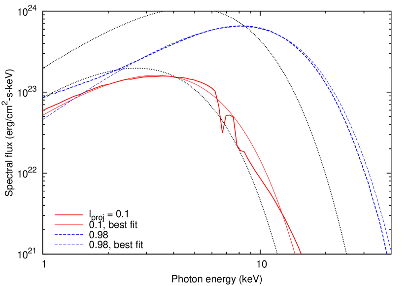
Figure 8.— Outgoing radiation spectrum, for atmospheres with solar composition, $g_{\rm base}=10^{14}~{}{\rm cm~{}s^{-2}}$, and $l_{\rm proj}=0.1$ or $0.98$. The best fit for each spectrum is shown as a thin line of the same color/pattern. The blackbody spectrum $B_{\nu}(T_{\rm eff,proj})$ for each atmosphere is also shown for comparison, as a black dotted line.

In this section we also plot the projected color correction (or spectral hardness) factor

$$f_{\rm c,proj}=\frac{T_{\rm c,proj}}{T_{\rm eff,proj}}\,,$$ (115)

where $T_{\rm c,proj}$ is the color temperature of the spectrum projected on to the base of the atmosphere [using Equations (111) and (112)] and $T_{\rm eff,proj}=(L_{\rm proj}/4\pi r_{\rm base}^{2}\sigma_{\rm SB})^{1/4}$ (London et al., 1986; Madej et al., 2004; Suleimanov et al., 2011b, 2012). For a given atmosphere, the color temperature is found by fitting the spectrum to a diluted Planck function

$$F_{\nu,\rm proj}\simeq wB_{\nu}(T_{\rm c,proj})\,;$$ (116)

for a perfect fit we would have $w=f_{\rm c,proj}^{-4}$. To fit our models to Equation (116) we use the “first” procedure of Suleimanov et al. (2011b), which consists of varying the parameters $w$ and $T_{\rm c,proj}$ to minimize the sum

$$\sum_{\rm n=1}^{N}\left[F_{\nu_{n},\rm proj}-wB_{\nu_{n}}(T_{\rm c,proj})\right]^{2}\,,$$ (117)

where $N$ is the number of frequency groups in the (RXTE PCA) energy band (3–20)$\times(1+z_{\rm base})$ keV [see Equation (101) for the conversion from frequency group to frequency]. Note that Suleimanov et al. treat the $1+z_{\rm base}$ factor slightly differently than we do, and therefore fit their models over a slightly different energy band; however, as they point out, such a change makes a negligible difference to the color correction values obtained. Figure 8 shows examples of spectra and their best fits from our models.

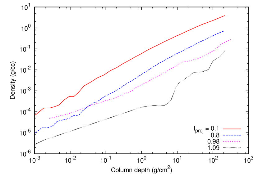
Figure 9.— Density as a function of column depth, for models with solar composition, $g_{\rm base}=10^{14}~{}{\rm cm~{}s^{-2}}$, and a variety of luminosity ratios. The quantity $r-r_{\rm base}$ (see Figure 1) at column depth $y=1~{}{\rm g~{}cm^{-2}}$ (optical depth $\tau_{F}^{\rm tot}\simeq 0.3$) is $130$, $850$, $3000$, and $4.4\times 10^{4}$ cm for the $l_{\rm proj}=0.1$, $0.8$, $0.98$, and $1.09$ model, respectively.

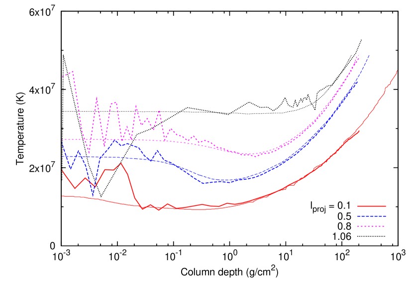
Figure 10.— Material temperature as a function of column depth, for atmospheres with solar composition, $g_{\rm base}=10^{14}~{}{\rm cm~{}s^{-2}}$, and a variety of luminosity ratios. The results from the model of Suleimanov et al. (2012) are shown as thin lines for comparison. The approximation $T_{\rm outer}$ from Equation (70) is $1.05$, $2.03$, $2.52$, and $3.21$ keV for the $l_{\rm proj}=0.1$, $0.5$, $0.8$, and $1.06$ atmosphere, respectively.

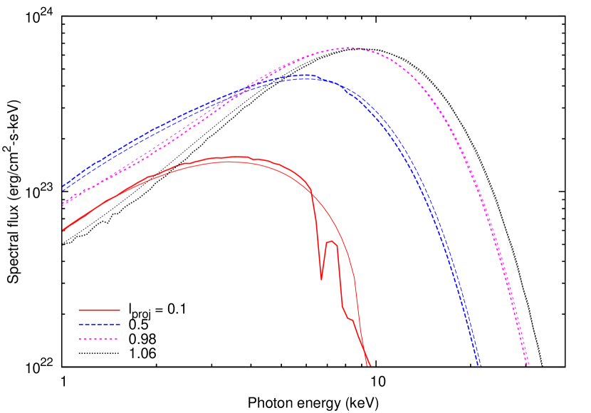
Figure 11.— Outgoing radiation spectrum, for atmospheres with solar composition, $g_{\rm base}=10^{14}~{}{\rm cm~{}s^{-2}}$, and a variety of luminosity ratios. The results from the model of Suleimanov et al. (2012) are shown for comparison, as thin lines with the same colors/patterns as our results.

Figures 9 and 10 show, respectively, examples of the density and temperature as a function of column depth from our models; while Figure 11 shows an example of the outgoing radiation spectrum. Figures 10 and 11 also show the results of Suleimanov et al. (2011b, 2012) for comparison (cf. figure 3 of either work). Our temperature profiles are qualitatively similar to those of Suleimanov et al.; compared to the results of Madej et al. (2004), however, our temperature profiles have a significantly larger dip at column depths of order unity (see, e.g., figure C.1 of Suleimanov et al., 2012). The profiles from both our work and that of Suleimanov et al. approach $T_{\rm outer}$ in the outer layers to within a few percent. Similarly, our spectra are qualitatively similar to those of Suleimanov et al. but differ substantially from those of Madej et al. (see below).

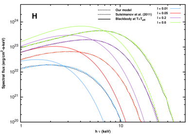
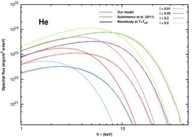
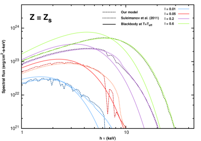
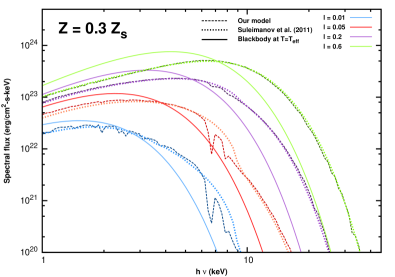
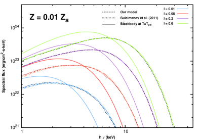
Figure 12.— Outgoing radiation spectrum for a variety of atmospheres (dashed lines). For comparison, the blackbody approximations are shown as solid lines and the results from the model of Suleimanov et al. (2012) are shown as dotted lines. Here the surface gravity is $g_{\rm base}=10^{14}~{}{\rm cm~{}s^{-2}}$.

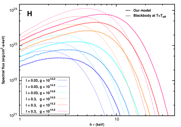
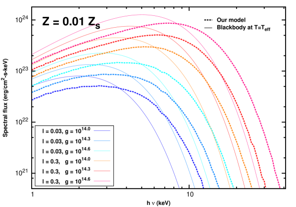
Figure 13.— Outgoing radiation spectrum for a variety of atmospheres (dashed lines). For comparison, the blackbody approximations are shown as solid lines. Here the composition is pure hydrogen (top panel) or modified solar (0.01$Z_{\odot}$; bottom panel).

Figure 12 shows a comparison of the outgoing spectra from our models and those of Suleimanov et al., for a variety of atmosphere compositions and luminosity ratios and a single gravity $\log(g_{\rm base}/{\rm cm~{}s^{-2}})=14.0$; Figure 13 shows a comparison for a variety of gravities. The spectra from the two works are very similar, except at the lowest luminosities and highest metallicities considered. In these low-$L$, high-$X_{\rm metal}$ cases, the spectra agree qualitatively but differ in the number of absorption features and the amplitudes of these features, owing to the different opacities used. As a consequence, the color corrections derived from these spectra are also different (see below). Conversely, the Madej et al. (2004) spectra have a qualitatively different shape, including a different peak and low- and high-frequency falloffs (again, compare our $g_{\rm base}=10^{14.3}~{}{\rm cm~{}s^{-2}}$, $l_{\rm proj}=0.5$ results to Madej et al.’s $T_{\rm eff}=2\times 10^{7}$ results; or see figure C.1 of Suleimanov et al. 2012). Note that if we had not included stimulated scattering in our models, our spectra would fall off faster with frequency at the high-frequency end and would not match as closely with the results of Suleimanov et al. (see Figure 7 in Section 4.3). On the other hand, for low frequencies our spectra with stimulated scattering differ by a few percent from those of Suleimanov et al., but without stimulated scattering are nearly exact; we attribute this difference to our approximate treatment of stimulated scattering (see the Appendix).

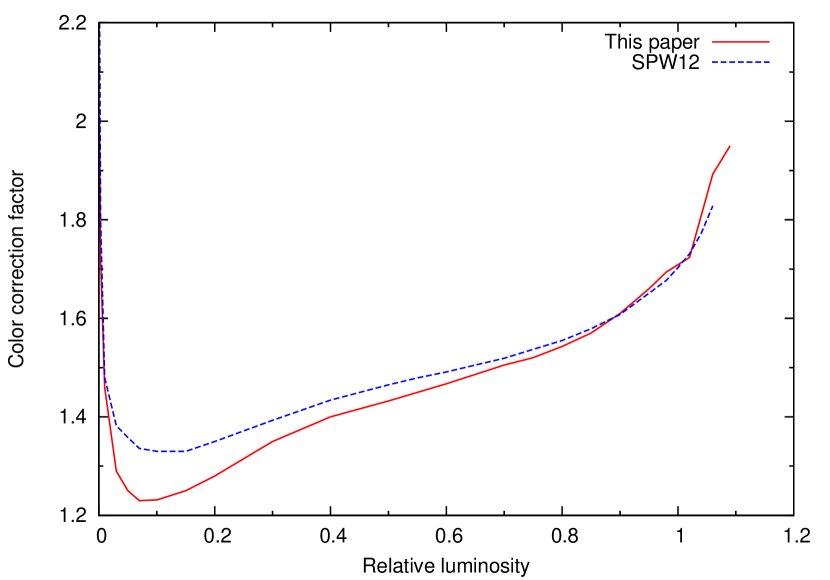
Figure 14.— Color correction factor as a function of relative luminosity for solar composition and $g_{\rm base}=10^{14}~{}{\rm cm~{}s^{-2}}$. The results from the model of Suleimanov et al. (2012) are shown as a dashed curve for comparison.

Figure 14 shows another comparison between our models and those of Suleimanov et al., in this case the color correction factor as a function of luminosity ratio for one atmosphere composition and gravity. A fixed $\{X\}$ and $g_{\rm base}$ corresponds to one burst on a hypothetical neutron star, assuming that the chemical composition in the atmosphere remains constant during the burst (Section 4.7). The curves from the two works are similar at high luminosity ratios, but differ by about 10% at low ratios ($l_{\rm proj}\alt 0.4$), due to the previously mentioned differences in the bound-free/bound-bound opacities used by each work. The large difference in $f_{\rm c,proj}$ for spectra that are very similar highlights the fact that at low luminosities a diluted Planck function is not a good fit to the model spectra (see Figure 8). Note that at the highest luminosities, the color corrections of either work differ from those of Madej et al. by about 5%.

6. Discussion/future directions

In this paper we model neutron star atmospheres at different times during an XRB. For each model we specify an atmosphere radius, composition, gravity, and equilibrium luminosity; guess the atmosphere structure and radiation field; and then evolve the atmosphere from our initial guess to the (quasi-)equilibrium by solving the time-dependent equations of radiation transfer and material energy along with the equation of hydrostatic balance (Section 2). This evolution proceeds in three steps, as described in Section 3: 1) We evolve the atmosphere to radiative equilibrium using the equations of radiation transfer and material energy. We solve these equations in a coupled manner, using an implicit Monte Carlo scheme that propagates photons in three dimensions; the photons interact with the atmosphere material via absorption/emission and scattering processes (Section 4 and the Appendix). 2) We adjust the material density profile using the equation of hydrostatic balance; to solve this equation we include contributions from both gas and radiation pressure. We then use step 1 to evolve the atmosphere to radiative equilibrium for this new hydrostatic state. 3) We repeat step 2 until a steady state is reached. If the luminosity from this steady state is not the desired value, we adjust the temperature at the base of the atmosphere and start the entire process over again. The validity of our piecewise method (in particular, the assumption that the atmosphere actually reaches a steady-state structure during an XRB) is discussed in Sections 4.1 and 4.5.

For accuracy we use absorption opacities from the OPLIB database; the additional bound-free and free-free transitions contained in the database lead to differences between our results and those of Suleimanov et al. (2011b, 2012) only at low luminosities and high metallicites (see Section 5). We also use Compton scattering and include the stimulated scattering contribution. Though stimulated scattering is not typically included in Monte Carlo calculations (because of the complexity it adds to the sampling algorithm for the scattered photon; but see Wienke et al. 2012), we find its inclusion necessary to obtain results that compare well with those of Suleimanov et al. (2012) (Sections 4.3 and 5). Additionally, we consider general relativistic effects within our model. In thin atmospheres ($r_{\rm surf}\alt 10^{5}$ cm), these effects can be added after calculation, as is done by, e.g., Madej et al. (2004) and Suleimanov et al. However, in the hottest XRBs, due to strong radiation pressure the atmosphere expands to many times its pre-burst size (e.g., Galloway et al., 2008), such that the change in gravitational field across the atmosphere is significant; in these atmospheres ($r_{\rm surf}\agt 10^{6}$ cm), general relativity must be included both for accuracy and for hydrostatic stability (Section 4.6).

We assume local thermodynamic equilibrium in the atmosphere, such that the material radiates as a Planck function according to Kirchoff’s law [Equation (10)]. The outgoing radiation spectrum from our models is non-Planckian, however, due to scattering and frequency-dependent absorption of the radiation field before it escapes the atmosphere (Section 4.2). At high temperatures, absorption is weak and the majority of the photons come from deep within the atmosphere; the color temperature of the outgoing spectrum is much larger than the effective temperature (i.e., $f_{\rm c,proj}\gg 1$; Section 5).

Our time-dependent, stochastic (Monte Carlo) approach to modeling XRB atmospheres differs from the time-independent, deterministic approaches of Madej et al. (2004), Suleimanov et al. (2012), and other groups, but our goals are the same: to find the equilibrium solution for a given set of atmosphere parameters. Our equilibrium spectra have the same qualitative shape as those of Suleimanov et al., and differ generally by less than 10%; the color correction factors compare even more closely (see Section 5). The fact that our results compare so well with those of Suleimanov et al. despite the different approaches, gives us more confidence in the validity of the methods and solutions of our group and theirs. On the other hand, our results do not compare well with those of Madej et al., which supports the conclusion of Suleimanov et al. that the former group’s results were in error.

Note that even though our models are time dependent, they do not represent the evolution of an atmosphere during a burst because we fix the temperature at the base of the atmosphere, and because we change the density profile in discrete jumps using a hydrostatic equation. To model the burst evolution we would need to use time-dependent temperature sources based on XRB energy generation models (e.g., Woosley et al., 2004; Malone et al., 2011, 2014), as well as solve the hydrodynamic equations together with our time-dependent radiation transfer and material energy equations (Section 4.5). We will consider these changes in future work.

We have attempted to include the relevant pieces of physics in our atmosphere models, but there is much we have left out for simplicity (see Section 4). For example, the composition of the atmosphere in our models is a free parameter and is uniform in space. In a real, X-ray-bursting neutron star atmosphere, the composition varies with radius, due to a combination of different processes: e.g., accretion, compositional mixing, and mass loss (Section 4.7). Not having an accurate model for the atmosphere composition introduces a large amount of uncertainty into our calculation results, since as we saw in Section 5, the composition strongly affects both the shape of the outgoing spectrum and the value of the color correction factor. While we compensate for this uncertainty by generating a variety of models with different compositions (see also Suleimanov et al., 2011b, 2012; Nättilä et al., 2015), this is not ideal since current model fits to observations can not distinguish between the possible compositions (e.g., Zamfir et al., 2012). In future work, we hope to implement into our atmosphere code a spatially varying composition that is motivated by detailed physics calculations of the convection zone (e.g., Woosley et al., 2004; Malone et al., 2014). As another example, the outer layers of our atmosphere are not in thermal equilibrium with the local radiation field. In the future we plan to implement opacities that account for that fact, at least crudely (Section 4.4).

In this paper we have attempted to reduce uncertainties in XRB models, but there are many other uncertainties associated with XRBs that we have not addressed or have addressed only partially (see Section 1). One uncertainty that we would like to address more fully in the future is how the apparent expansion and contraction of the atmosphere, characterized by the observed blackbody radius $R_{\rm bb}=\left(L_{\infty}/4\pi\sigma_{\rm SB}T_{\rm bb}^{4}\right)^{1/2}$ and color temperature $T_{\rm bb}$ (see Lewin et al. 1993 for a review), correlates with the actual expansion and contraction. During a PRE burst, $R_{\rm bb}$ grows to ${\rm a~{}few}\times 10$ km, then decays to a minimum value $\sim 10$ km, then in some cases grows by ${\rm a~{}few}\times 10\%$, before finally leveling off (e.g., 4U 1724–307; see Galloway et al., 2008). Presumably the growth and decay of $R_{\rm bb}$ is correlated with the expansion and contraction of the photosphere; however, this is complicated by the fact that $R_{\rm bb}$ also depends on the color correction factor, since the spectrum is not a blackbody. In particular, since $R_{\rm bb}\propto f_{\rm c,proj}^{-2}$, if during contraction $f_{\rm c,proj}^{2}$ decays faster than the photosphere radius does, the blackbody radius will actually grow. This could mean that the time when $R_{\rm bb}$ reaches a minimum, the so-called “touchdown” point, is not the same as the time when the photosphere has returned to its pre-burst radius (Steiner et al., 2010; Suleimanov et al., 2011b; Steiner et al., 2013). Even if the touchdown point corresponds to a fully contracted photosphere, it is difficult to derive constraints on the neutron star mass and radius from observations only, without a detailed model of the atmosphere behavior at touchdown. For example, some XRB groups (e.g., Lewin et al., 1993; Özel et al., 2009) argue that the luminosity at touchdown is given by the Eddington luminosity $L_{\rm Edd}$ [Equation (52)], since above this luminosity the atmosphere will be hydrodynamically unstable and therefore highly extended. However, one can not use the Thomson approximation $\kappa_{\rm Th}$ for the opacity in $L_{\rm Edd}$, since for neutron stars near the Eddington limit the atmosphere will be hot and the true opacity $\kappa_{F}^{\rm tot}\ll\kappa_{\rm Th}$ [Equation (63)]. Instead, for each atmosphere under consideration, one must self-consistently find $L_{\rm Edd}$ at the point where the atmosphere is on the edge of stability. We are currently using our XRB code to model extended atmospheres like those described by Paczynski & Anderson (1986) (see Section 3.2), with the goal of obtaining spectra and color correction factors at luminosity ratios all the way up to the value at touchdown (which could potentially be as large as $1+z_{\rm base}$; cf. Lewin et al., 1993; Suleimanov et al., 2011b). Whether this can be done with a hydrostatic code, or whether the full hydrodynamic equations must be solved, remains to be seen.

Appendix A Monte Carlo method for Compton scattering

Here we describe our method for implementing Compton scattering within the Monte Carlo framework, first when stimulated scattering is ignored (Section A.1), and then when it is included (Section A.2). Our method is similar to that of Canfield et al. (1987), but we sample from a Maxwell-Boltzmann electron distribution rather than a relativistic one. We refer to Kahn (1956); Everett & Cashwell (1983); Kalos & Whitlock (1986) for details on sampling from Maxwell-Boltzmann and Klein-Nishina distributions.

A.1. Ignoring stimulated scattering

To determine the probability of a scattering event occurring for a specific Monte Carlo particle in the simulation, our code needs to know the value of the scattering opacity $\kappa_{\nu}^{\rm sc}$. Ignoring stimulated scattering, Equation (31) becomes

$$\kappa_{\nu}^{\rm sc}=\frac{Y_{e}}{m_{u}}\int_{0}^{\infty}4\pi p^{2}dp\,f(p)\int_{-1}^{1}d\zeta\frac{1-\beta\zeta}{2}\sigma_{\rm KN}(\nu_{0})$$ (A1)

with

$$\sigma_{\rm KN}(\nu_{0})={} \int_{0}^{2\pi}\frac{d\zeta_{\perp}}{2\pi}\int_{0}^{2\pi}\frac{d\eta_{0,\perp}}{2\pi}\int_{\nu_{0}/(1+2x_{0})}^{\nu_{0}}d\nu^{\prime}_{0}\sigma_{\rm KN}(\nu_{0}\rightarrow\nu^{\prime}_{0})$$ (A2)

$$={} \frac{3\sigma_{\rm Th}}{4x_{0}^{2}}\left[2+\frac{x_{0}^{2}(1+x_{0})}{(1+2x_{0})^{2}}+\frac{x_{0}^{2}-2x_{0}-2}{2x_{0}}\ln(1+2x_{0})\right]$$ (A3)

(e.g., Rybicki & Lightman, 1986). Note that $\nu_{0}$, $\nu$, $\zeta$, $\gamma$, $\beta$, and $p$ do not depend on $\zeta_{\perp}$ and $\eta_{0,\perp}$ [Equations (19)–(21)], such that $\zeta_{\perp}$ and $\eta_{0,\perp}$ could be integrated out of Equation (A2); however, we keep these latter variables in the equation to demonstrate how our Monte Carlo sampling algorithm works. We can express the integrand on the right-hand side of Equation (A1) as a joint probability density function

$$P(\zeta,p)=P(\zeta|p)P(p)$$ (A4)

times a rejection factor $R$ times a constant $C$:

$$P(p)=4\pi p^{2}f(p)$$ (A5)

with

$$\int_{0}^{\infty}P(p)\,dp=1\,,$$ (A6)

$$P(\zeta|p)=\frac{1}{2}(1-\beta\zeta)$$ (A7)

with

$$\int_{-1}^{1}d\zeta\,P(\zeta|p)=1\,,$$ (A8)

$$R=\frac{\sigma_{\rm KN}(\nu_{0})}{\sigma_{\rm Th}}\leq 1\,,$$ (A9)

and therefore

$$C=\sigma_{\rm Th}\,.$$ (A10)

We find the value of the integral in Equation (A1) through rejection sampling: We first sample from $P(p)$, a Maxwell-Boltzmann distribution (e.g., Everett & Cashwell, 1983; Kalos & Whitlock, 1986). Given $p$, we then sample from $P(\zeta|p)$, by generating a random variable $\xi_{1}\in[0,1]$ and solving for $\zeta$ using

$$\int_{-1}^{\zeta}d\bar{\zeta}\,P(\bar{\zeta}|p)=\frac{1}{2}\left[\zeta+1-\frac{\beta}{2}\left(\zeta^{2}-1\right)\right]=\xi_{1}\,.$$ (A11)

Finally, we generate another random variable $\xi_{2}\in[0,1]$, and if $\xi_{2}>R$ we reject our $\{p,\zeta\}$ sample set. This process is repeated many times, and we record the fraction of the total sample sets that are accepted, $f_{\rm accept}$. After sufficient iterations such that $f_{\rm accept}$ is converged ($10^{4}$ iterations or more), the integral is given by $C\times f_{\rm accept}$, and $\kappa_{\nu}^{\rm sc}$ is $Y_{e}/m_{u}$ times that. A table of $\kappa_{\nu}^{\rm sc}$ values is calculated for a range of $\nu$ and $T$, analogous to the table of absorption opacities. The table generation is done only once, at the beginning of the simulation. Note that we could instead use the scattering opacities from the OPLIB database, also evaluated using Equation (A1). However, we can not use the OPLIB database for stimulated scattering (Section A.2), so we use the above method for consistency.

When a scattering event occurs, the code also needs to know the properties of the Monte Carlo particle after scattering, so that it can determine the momentum and energy transferred between the particle and the atmosphere material and can further transport the particle. We first sample from $P(p)$ and $P(\zeta|p)$; then if $\xi_{2}>R$, reject the $\{p,\zeta\}$ set and resample until $\xi_{2}\leq R$. Note that unlike above, we only do this procedure once (or rather, until the first time $\xi_{2}\leq R$) for each scattering event. Then the Klein-Nishina distribution is sampled (Kahn, 1956; Everett & Cashwell, 1983) to find $\nu^{\prime}_{0}$ and $\eta_{0}$, and $\zeta_{\perp}$ and $\eta_{0,\perp}$ are each sampled uniformly in $[0,2\pi]$. The photon direction after scattering $\hat{\Omega}^{\prime}$ is found through Lorentz transformations and three-dimensional rotations: We first find $\hat{n}$ from $\hat{\Omega}$, rotating $\hat{\Omega}$ by an angle $\arccos(\zeta)$ about the vector $\hat{\Omega}_{\perp 1}$, where $\hat{\Omega}_{\perp 1}$ is some direction orthogonal to $\hat{\Omega}$, to get $\hat{n}_{1}$; and then rotating $\hat{n}_{1}$ by an angle $\zeta_{\perp}$ about the vector $\hat{\Omega}$. From Rodrigues’ rotation formula we have

$$\hat{n}_{1}=\zeta\hat{\Omega}+\sqrt{1-\zeta^{2}}\hat{\Omega}_{\perp 2}$$ (A12)

and

$$\hat{n}=\zeta\hat{\Omega}+\sqrt{1-\zeta^{2}}\sin\zeta_{\perp}\hat{\Omega}_{\perp 1}+\sqrt{1-\zeta^{2}}\cos\zeta_{\perp}\hat{\Omega}_{\perp 2}\,,$$ (A13)

where $\hat{\Omega}_{\perp 2}$ is orthogonal to both $\hat{\Omega}_{\perp 1}$ and $\hat{\Omega}$. For simplicity we choose $\hat{\Omega}_{\perp 1}$ to be in the $x$-$y$ plane, such that in Cartesian coordinates

$$\hat{n}=\left(\begin{array}[]{c}\zeta\Omega_{x}+\frac{\sqrt{1-\zeta^{2}}}{\sqrt{1-\Omega_{z}^{2}}}\left(-\sin\zeta_{\perp}\Omega_{y}+\cos\zeta_{\perp}\Omega_{x}\Omega_{z}\right)\\ \zeta\Omega_{y}+\frac{\sqrt{1-\zeta^{2}}}{\sqrt{1-\Omega_{z}^{2}}}\left(\sin\zeta_{\perp}\Omega_{x}+\cos\zeta_{\perp}\Omega_{y}\Omega_{z}\right)\\ \zeta\Omega_{z}-\sqrt{1-\zeta^{2}}\sqrt{1-\Omega_{z}^{2}}\cos\zeta_{\perp}\end{array}\right)$$ (A14)

(unless $\hat{\Omega}\equiv\pm\hat{z}$, in which case we choose $\hat{n}=\pm\zeta\hat{z}+\sqrt{1-\zeta^{2}}\sin\zeta_{\perp}\hat{y}+\sqrt{1-\zeta^{2}}\cos\zeta_{\perp}\hat{x}$). Note that the ambiguity in the value of $\sin(\arccos(\zeta))=\pm\sqrt{1-\zeta^{2}}$ and the choice of $\hat{\Omega}_{\perp 1}$, is accounted for by the fact that $\zeta_{\perp}$ is a random number between $0$ and $2\pi$; we can define $\arccos(\zeta)$ over any domain and choose any orthogonal vector $\hat{\Omega}_{\perp 1}$ and still cover all possible directions for $\hat{n}$. After finding $\hat{n}$ we find $\hat{\Omega}_{0}$ (the photon direction pre-scattering and in the electron rest frame), using the Lorentz angle transformations (e.g., Rybicki & Lightman, 1986)

$$\zeta_{0}=\frac{\zeta-\beta}{1-\beta\zeta}=\frac{\nu}{\nu_{0}}\gamma(\zeta-\beta)$$ (A15)

and

$$\zeta_{0,\perp}=\frac{\zeta_{\perp}}{\gamma(1-\beta\zeta)}=\frac{\nu}{\nu_{0}}\zeta_{\perp}\,;$$ (A16)

combined, these give

$$\hat{\Omega}_{0}=\frac{\nu}{\nu_{0}}\left\{\hat{\Omega}+[(\gamma-1)\zeta-\gamma\beta]\hat{n}\right\}\,.$$ (A17)

We find $\hat{\Omega}^{\prime}_{0}$ (the photon direction post-scattering and in the electron rest frame) using Rodrigues’ rotation formula in the same manner as described above to get

$$\hat{\Omega}^{\prime}_{0}=\left(\begin{array}[]{c}\eta_{0}\Omega_{0,x}+\frac{\sqrt{1-\eta_{0}^{2}}}{\sqrt{1-\Omega_{0,z}^{2}}}\left(-\sin\eta_{0,\perp}\Omega_{0,y}+\cos\eta_{0,\perp}\Omega_{0,x}\Omega_{0,z}\right)\\ \eta_{0}\Omega_{0,y}+\frac{\sqrt{1-\eta_{0}^{2}}}{\sqrt{1-\Omega_{0,z}^{2}}}\left(\sin\eta_{0,\perp}\Omega_{0,x}+\cos\eta_{0,\perp}\Omega_{0,y}\Omega_{0,z}\right)\\ \eta_{0}\Omega_{0,z}-\sqrt{1-\eta_{0}^{2}}\sqrt{1-\Omega_{0,z}^{2}}\cos\eta_{0,\perp}\end{array}\right)\,.$$ (A18)

Finally, we find $\hat{\Omega}^{\prime}$ using Lorentz angle transformations in the same manner as above (but transforming back to the neutron star frame) to get

$$\hat{\Omega}^{\prime}=\frac{\nu^{\prime}_{0}}{\nu^{\prime}}\left\{\hat{\Omega}_{0}^{\prime}+[(\gamma-1)\zeta^{\prime}_{0}+\gamma\beta]\hat{n}\right\}\,,$$ (A19)

where

$$\nu^{\prime}=\gamma\nu_{0}^{\prime}(1+\beta\zeta^{\prime}_{0})$$ (A20)

and

$$\zeta^{\prime}_{0}=\hat{\Omega}^{\prime}_{0}\cdot\hat{n}\,.$$ (A21)

A.2. Including stimulated scattering

To find $\kappa_{\nu}^{\rm sc}$ when stimulated scattering is included, we must solve Equation (31) as written. Here we can not integrate $\nu^{\prime}_{0}$ out of the scattering equation (since the integral with respect to $\nu^{\prime}_{0}$ is not analytic), so we express the integrand on the right-hand side of the equation as

$$P(\nu^{\prime}_{0},\eta_{0,\perp},\zeta_{\perp},\zeta,p)=P(\nu^{\prime}_{0}|\eta_{0,\perp},\zeta_{\perp},\zeta,p)P(\eta_{0,\perp}|\zeta_{\perp},\zeta,p)P(\zeta_{\perp}|\zeta,p)P(\zeta|p)P(p)$$ (A22)

times a rejection factor $R$ times a constant $C$; $P(p)$ and $P(\zeta|p)$ are as in Equations (A5) and (A7),

$$P(\zeta_{\perp}|\zeta,p)=\frac{1}{2\pi}$$ (A23)

with

$$\int_{0}^{2\pi}P(\zeta_{\perp}|\zeta,p)\,d\zeta_{\perp}=1\,,$$ (A24)

$$P(\eta_{0,\perp}|\zeta_{\perp},\zeta,p)=\frac{1}{2\pi}$$ (A25)

with

$$\int_{0}^{2\pi}P(\eta_{0,\perp}|\zeta_{\perp},\zeta,p)\,d\eta_{0,\perp}=1\,,$$ (A26)

$$P(\nu^{\prime}_{0},\eta_{0,\perp},\zeta_{\perp},\zeta,p)=\frac{\sigma_{\rm KN}(\nu_{0}\rightarrow\nu^{\prime}_{0})}{\sigma_{\rm KN}(\nu_{0})}$$ (A27)

with

$$\int_{\nu_{0}/(1+2x_{0})}^{\nu_{0}}d\nu^{\prime}_{0}\,P(\nu^{\prime}_{0}|\eta_{0,\perp},\zeta_{\perp},\zeta,p)=1\,,$$ (A28)

$$R=\frac{1+c^{2}I_{\nu^{\prime}}(\hat{\Omega}^{\prime})/2h{\nu^{\prime}}^{3}}{1+[\exp(Ah\nu/k_{\rm B}T)-1]^{-1}}\frac{\sigma_{\rm KN}(\nu_{0})}{\sigma_{\rm Th}}\alt 1\,,$$ (A29)

and therefore

$$C=\left[1+\frac{1}{\exp(Ah\nu/k_{\rm B}T)-1}\right]\sigma_{\rm Th}\,.$$ (A30)

Here $A\leq 1$ is a parameter chosen by the user (see below). To reduce the noise on $I_{\nu}(\hat{\Omega})$ we average this quantity over 1000 time steps (cf. Section 3.3); we therefore also only recalculate the $\kappa_{\nu}^{\rm sc}$ table every 1000 time steps, to save calculation time. We sample the various probability density functions above as in Section A.1 [$P(\nu^{\prime}_{0}|\eta_{0,\perp},\zeta_{\perp},\zeta,p)$ is the Klein-Nishina distribution]; then repeat the sampling many times until we obtain a converged value of $f_{\rm accept}$, after which we set $\kappa_{\nu}^{\rm sc}=(Y_{e}/m_{u})Cf_{\rm accept}$. For a single scattering event, we sample the various functions once; then if $\xi>R$ reject the sample set and resample until $\xi\leq R$.

The approximation in our treatment of stimulated scattering is that $R$ in Equation (A29) never exceeds unity. The inequality

$$\sigma_{\rm KN}(x)\leq\sigma_{\rm Th}$$ (A31)

is always true, but

$$\frac{c^{2}I_{\nu^{\prime}}(\hat{\Omega}^{\prime})}{2h{\nu^{\prime}}^{3}}\leq\frac{1}{\exp(Ah\nu/k_{\rm B}T)-1}$$ (A32)

is an empirical relation (chosen because $c^{2}I_{\nu}/2h\nu^{3}=[\exp(h\nu/k_{\rm B}T)-1]^{-1}$ for a Planckian radiation field) that is only absolutely true in the limit $A\rightarrow 0$. In practical terms, the parameter $A$ should not be too small or the number of rejections will be very large and the Monte Carlo integration will take a long time; but it should not be too large or the error in the result will be large. For our XRB atmosphere calculations, we chose $A=0.2$ for reasonably fast integration time and a rejection factor Equation (A29) that exceeds unity less than 1 time in $10^{5}$.

References

- Asplund et al. (2009) Asplund, M., Grevesse, N., Sauval, A. J., & Scott, P. 2009, ARA&A, 47, 481
- Busquet (1993) Busquet, M. 1993, Physics of Fluids B, 5, 4191
- Busquet et al. (2009) Busquet, M., Colombant, D., Klapisch, M., Fyfe, D., & Gardner, J. 2009, High Energy Density Physics, 5, 270
- Cackett et al. (2010) Cackett, E. M., Brown, E. F., Miller, J. M., & Wijnands, R. 2010, ApJ, 720, 1325
- Canfield et al. (1987) Canfield, E., Howard, W. M., & Liang, E. P. 1987, ApJ, 323, 565
- Castor (2004) Castor, J. I. 2004, Radiation Hydrodynamics (Cambridge: Cambridge University Press)
- Catuneanu et al. (2013) Catuneanu, A., Heinke, C. O., Sivakoff, G. R., Ho, W. C. G., & Servillat, M. 2013, ApJ, 764, 145
- Chang & Bildsten (2003) Chang, P., & Bildsten, L. 2003, ApJ, 585, 464
- Damen et al. (1990) Damen, E., Magnier, E., Lewin, W. H. G., et al. 1990, A&A, 237, 103
- Demorest et al. (2010) Demorest, P. B., Pennucci, T., Ransom, S. M., Roberts, M. S. E., & Hessels, J. W. T. 2010, Nature, 467, 1081
- Densmore et al. (2007) Densmore, J. D., Urbatsch, T. J., Evans, T. M., & Buksas, M. W. 2007, Journal of Computational Physics, 222, 485
- Ebisuzaki (1987) Ebisuzaki, T. 1987, PASJ, 39, 287
- Ebisuzaki & Nakamura (1988) Ebisuzaki, T., & Nakamura, N. 1988, ApJ, 328, 251
- Eisenberger & Platzman (1970) Eisenberger, P., & Platzman, P. M. 1970, Phys. Rev. A, 2, 415
- Everett & Cashwell (1983) Everett, C. J., & Cashwell, E. D. 1983, A Third Monte Carlo Sampler, Los Alamos Technical Report LA-9721-MS, LANL
- Fleck & Cummings (1971) Fleck, Jr., J. A., & Cummings, J. D. 1971, Journal of Computational Physics, 8, 313
- Frey et al. (2013) Frey, L. H., Even, W., Whalen, D. J., et al. 2013, ApJS, 204, 16
- Galloway et al. (2004) Galloway, D. K., Cumming, A., Kuulkers, E., et al. 2004, ApJ, 601, 466
- Galloway & Lampe (2012) Galloway, D. K., & Lampe, N. 2012, ApJ, 747, 75
- Galloway et al. (2008) Galloway, D. K., Muno, M. P., Hartman, J. M., Psaltis, D., & Chakrabarty, D. 2008, ApJS, 179, 360
- Glendenning & Schaffner-Bielich (1998) Glendenning, N. K., & Schaffner-Bielich, J. 1998, Physical Review Letters, 81, 4564
- Guillot et al. (2013) Guillot, S., Servillat, M., Webb, N. A., & Rutledge, R. E. 2013, ApJ, 772, 7
- Heinke et al. (2006) Heinke, C. O., Rybicki, G. B., Narayan, R., & Grindlay, J. E. 2006, ApJ, 644, 1090
- Ho & Heinke (2009) Ho, W. C. G., & Heinke, C. O. 2009, Nature, 462, 71
- Ho et al. (2007) Ho, W. C. G., Kaplan, D. L., Chang, P., van Adelsberg, M., & Potekhin, A. Y. 2007, MNRAS, 375, 821
- Huba (2013) Huba, J. D. 2013, NRL plasma formulary, revised, Naval Research Lab. Report NRL/PU/6790-16-614, Naval Research Laboratory
- Joss (1977) Joss, P. C. 1977, Nature, 270, 310
- Kahn (1956) Kahn, H. 1956, Applications of Monte Carlo, U.S.A.E.C Report AECU-3259, Rand Corporation
- Kajava et al. (2016) Kajava, J. J. E., Nättilä, J., Poutanen, J., et al. 2016, ArXiv e-prints, arXiv:1608.06801
- Kalos & Whitlock (1986) Kalos, M. H., & Whitlock, P. A. 1986, Monte Carlo methods. (New York: John Wiley & Sons)
- Klochkov et al. (2015) Klochkov, D., Suleimanov, V., Pühlhofer, G., et al. 2015, A&A, 573, A53
- Kurkela et al. (2010) Kurkela, A., Romatschke, P., & Vuorinen, A. 2010, Phys. Rev. D, 81, 105021
- Lackey et al. (2006) Lackey, B. D., Nayyar, M., & Owen, B. J. 2006, Phys. Rev. D, 73, 024021
- Lai (2001) Lai, D. 2001, Reviews of Modern Physics, 73, 629
- Lattimer (2012) Lattimer, J. M. 2012, Annual Review of Nuclear and Particle Science, 62, 485
- Lattimer & Prakash (2004) Lattimer, J. M., & Prakash, M. 2004, Science, 304, 536
- Lattimer & Prakash (2007) —. 2007, Phys. Rep., 442, 109
- Lattimer & Steiner (2014) Lattimer, J. M., & Steiner, A. W. 2014, ApJ, 784, 123
- Lewin et al. (1993) Lewin, W. H. G., van Paradijs, J., & Taam, R. E. 1993, Space Sci. Rev., 62, 223
- Lindquist (1966) Lindquist, R. W. 1966, Annals of Physics, 37, 487
- London et al. (1986) London, R. A., Taam, R. E., & Howard, W. M. 1986, ApJ, 306, 170
- Madej et al. (2004) Madej, J., Joss, P. C., & Różańska, A. 2004, ApJ, 602, 904
- Magee et al. (1995) Magee, N. H., Abdallah, Jr., J., Clark, R. E. H., et al. 1995, in Astronomical Society of the Pacific Conference Series, Vol. 78, Astrophysical Applications of Powerful New Databases, ed. S. J. Adelman & W. L. Wiese, 51
- Majczyna et al. (2005) Majczyna, A., Madej, J., Joss, P. C., & Różańska, A. 2005, A&A, 430, 643
- Malone et al. (2011) Malone, C. M., Nonaka, A., Almgren, A. S., Bell, J. B., & Zingale, M. 2011, ApJ, 728, 118
- Malone et al. (2014) Malone, C. M., Zingale, M., Nonaka, A., Almgren, A. S., & Bell, J. B. 2014, ApJ, 788, 115
- Mihalas (1978) Mihalas, D. 1978, Stellar atmospheres /2nd edition/ (San Francisco: W. H. Freeman and Co.)
- Mihalas & Mihalas (1984) Mihalas, D., & Mihalas, B. W. 1984, Foundations of radiation hydrodynamics (New York: Oxford University Press)
- Miller (2013) Miller, M. C. 2013, ArXiv e-prints, arXiv:1312.0029
- Miller et al. (2011) Miller, M. C., Boutloukos, S., Lo, K. H., & Lamb, F. K. 2011, in Fast X-ray Timing and Spectroscopy at Extreme Count Rates (HTRS 2011)
- Misner et al. (1973) Misner, C. W., Thorne, K. S., & Wheeler, J. A. 1973, Gravitation (New York: W. H. Freeman and Company)
- Nättilä et al. (2015) Nättilä, J., Suleimanov, V. F., Kajava, J. J. E., & Poutanen, J. 2015, A&A, 581, A83
- Ofengeim et al. (2015) Ofengeim, D. D., Kaminker, A. D., Klochkov, D., Suleimanov, V., & Yakovlev, D. G. 2015, MNRAS, 454, 2668
- Özel et al. (2010) Özel, F., Baym, G., & Güver, T. 2010, Phys. Rev. D, 82, 101301
- Özel et al. (2009) Özel, F., Güver, T., & Psaltis, D. 2009, ApJ, 693, 1775
- Paczynski & Anderson (1986) Paczynski, B., & Anderson, N. 1986, ApJ, 302, 1
- Pavlov et al. (1991) Pavlov, G. G., Shibanov, I. A., & Zavlin, V. E. 1991, MNRAS, 253, 193
- Potekhin et al. (1997) Potekhin, A. Y., Chabrier, G., & Yakovlev, D. G. 1997, A&A, 323, 415
- Poutanen et al. (2014) Poutanen, J., Nättilä, J., Kajava, J. J. E., et al. 2014, MNRAS, 442, 3777
- Rajagopal & Romani (1996) Rajagopal, M., & Romani, R. W. 1996, ApJ, 461, 327
- Rutledge et al. (1999) Rutledge, R. E., Bildsten, L., Brown, E. F., Pavlov, G. G., & Zavlin, V. E. 1999, ApJ, 514, 945
- Rybicki & Lightman (1986) Rybicki, G. B., & Lightman, A. P. 1986, Radiative Processes in Astrophysics (Wiley-VCH)
- Sampson (1959) Sampson, D. H. 1959, ApJ, 129, 734
- Schulze et al. (2006) Schulze, H.-J., Polls, A., Ramos, A., & Vidaña, I. 2006, Phys. Rev. C, 73, 058801
- Shaposhnikov & Titarchuk (2002) Shaposhnikov, N., & Titarchuk, L. 2002, ApJ, 567, 1077
- Steiner et al. (2010) Steiner, A. W., Lattimer, J. M., & Brown, E. F. 2010, ApJ, 722, 33
- Steiner et al. (2013) —. 2013, ApJ, 765, L5
- Strohmayer & Bildsten (2006) Strohmayer, T. E., & Bildsten, L. 2006, in Compact Stellar X-ray Sources, ed. W. Lewin & M. van der Klis (Cambridge: Cambridge University Press), 113
- Suleimanov et al. (2011a) Suleimanov, V., Poutanen, J., Revnivtsev, M., & Werner, K. 2011a, ApJ, 742, 122
- Suleimanov et al. (2011b) Suleimanov, V., Poutanen, J., & Werner, K. 2011b, A&A, 527, A139
- Suleimanov et al. (2012) —. 2012, A&A, 545, A120
- Thorne (1967) Thorne, K. S. 1967, in High Energy Astrophysics, Volume 3, ed. C. Dewitt, E. Schatzman, & P. Véron, 259
- Thorne (1977) Thorne, K. S. 1977, ApJ, 212, 825
- van Paradijs (1979) van Paradijs, J. 1979, ApJ, 234, 609
- van Paradijs et al. (1990) van Paradijs, J., Dotani, T., Tanaka, Y., & Tsuru, T. 1990, PASJ, 42, 633
- van Paradijs & Lewin (1986) van Paradijs, J., & Lewin, H. G. 1986, A&A, 157, L10
- Weinberg et al. (2006) Weinberg, N. N., Bildsten, L., & Schatz, H. 2006, ApJ, 639, 1018
- Wienke (1985) Wienke, B. R. 1985, A&A, 152, 336
- Wienke et al. (2012) Wienke, B. R., Budge, K. G., Chang, J. H., Dahl, J. A., & Hungerford, A. L. 2012, J. Quant. Spec. Radiat. Transf., 113, 150
- Wollaber (2008) Wollaber, A. B. 2008, PhD thesis, University of Michigan
- Woosley et al. (2004) Woosley, S. E., Heger, A., Cumming, A., et al. 2004, ApJS, 151, 75
- Zamfir et al. (2012) Zamfir, M., Cumming, A., & Galloway, D. K. 2012, ApJ, 749, 69