A Concurrent Global-Local Numerical Method for Multiscale PDEs

Abstract.

We present a new hybrid numerical method for multiscale partial differential equations, which simultaneously captures the global macroscopic information and resolves the local microscopic events over regions of relatively small size. The method couples concurrently the microscopic coefficients in the region of interest with the homogenized coefficients elsewhere. The cost of the method is comparable to the heterogeneous multiscale method, while being able to recover microscopic information of the solution. The convergence of the method is proved for problems with bounded and measurable coefficients, while the rate of convergence is established for problems with rapidly oscillating periodic or almost-periodic coefficients. Numerical results are reported to show the efficiency and accuracy of the proposed method.

1. Introduction

Consider the elliptic problem with Dirichlet boundary condition

(1.1) $$\left\{\begin{aligned} -\operatorname{div}\left(a^{\,\varepsilon}(x)\nabla u^{\varepsilon}(x)\right)&=f(x),\qquad&&x\in D\subset\mathbb{R}^{n},\\ u^{\varepsilon}(x)&=0,\qquad&&x\in\partial D,\end{aligned}\right.$$

where $D$ is a bounded domain in $\mathbb{R}^{n}$ and $\varepsilon$ is a small parameter that signifies explicitly the multiscale nature of the coefficient $a^{\,\varepsilon}$. We assume $a^{\,\varepsilon}$ belongs to a set $\mathcal{M}(\lambda,\varLambda;D)$ that is defined as

$$\mathcal{M}(\lambda,\varLambda;D){:}=\Bigl{\{}a\in[L^{\infty}(D)]^{n\times n}\;\mid\; \xi\cdot a(x)\xi\geq\lambda\left\lvert\xi\right\rvert^{2},\xi\cdot a(x)\xi\geq(1/\varLambda)\left\lvert a(x)\xi\right\rvert^{2}$$

$$\quad\text{for any\;}\xi\in\mathbb{R}^{n}\text{\;and\;}a.e.\;x\text{\;in\;}D\;\Bigr{\}},$$

where $\left\lvert\cdot\right\rvert$ denotes the Euclidean norm in $\mathbb{R}^{n}$. Note that the coefficients $a^{\,\varepsilon}$ in $\mathcal{M}(\lambda,\varLambda;D)$ are not necessarily symmetric.

The large scale behavior of the solution of (1.1) is well understood by the theory of homogenization. In the sense of H-convergence due to Murat and Tartar [Tartar:2009, Theorem 6.5] and [MuratTartar:1997], for every $a^{\,\varepsilon}\in\mathcal{M}(\lambda,\varLambda;D)$ and $f\in H^{-1}(D)$ the sequence of solutions $\{u^{\varepsilon}\}$ of (1.1) satisfies

$$u^{\varepsilon} \rightharpoonup u_{0}\qquad \text{weakly in}\quad H_{0}^{1}(D),\,\text{and}$$

$$a^{\,\varepsilon}\nabla u^{\varepsilon} \rightharpoonup\mathcal{A}\nabla u_{0}\qquad \text{weakly in}\quad[L^{2}(D)]^{n},$$

where $u_{0}$ is the solution of a homogenized problem

(1.2) $$\left\{\begin{aligned} -\operatorname{div}\left(\mathcal{A}(x)\nabla u_{0}(x)\right)&=f(x),\qquad&&x\in D,\\ u_{0}(x)&=0,\qquad&&x\in\partial D,\end{aligned}\right.$$

with the homogenized coefficient $\mathcal{A}\in\mathcal{M}(\lambda,\varLambda;D)$.

For multiscale PDEs as (1.1), the quantities of interest include the macroscopic behavior of the solution and also the microscopic information (local fluctuation) of the solution [Ebook:2011]. Many numerical approaches based on the idea of homogenization have been proposed and thoroughly studied in the literature, such as the multiscale finite element method [HouWu:1997] and the heterogeneous multiscale method (HMM) [EEnquist:2003].

In this work, our focus is the scenario where the microscopic coefficient $a^{\,\varepsilon}$ is only available in part of the domain, while outside the region, only a coarse information is available about the coefficient field. More specifically, we only assume the knowledge of the homogenized coefficients outside a small region of the domain. The question is that given this information, whether it is still possible to recover the macroscopic behavior of the solution, together with resolving the local fluctuation of the solution, where the detailed information of the coefficient is known.

Several numerical approaches have been developed in recent years for such scenario. Those methods can be roughly put into two categories.

The first class is the global-local approach firstly proposed in [OdenVemaganti:2000, OdenVemaganti:2001], and further developed in [EEnquist:2003, EMingZhang:2005, BabuskaLipton:2011, BabuskaMotamedTempone:2014]. This is a two stage method: One first computes the homogenized global solution $u_{0}$ over the whole domain and then one finds the local fluctuation by solving an extra problem on a local part of the domain. The homogenized solution may be used as boundary condition in solving the local problem or be used to provide information on the fine scale based on a $L^{2}$-projection. The convergence of this approach has been investigated numerically in [MingYue:2006] for problems with many scales, within the HMM framework [HMMreview1, HMMreview2]. This approach has also been critically reviewed in [BabuskaLiptonStuebner:2008], where in particular the choice of the local approximation space was investigated.

Another class of method is based on the idea of domain decomposition, which concerns handshaking multiple operators acting on different parts of the physical domain. Those operators may be either the restrictions of the same governing differential operators to the overlapping or non-overlapping sub-domains [DuGunzburger:2000, Gervasio:2001, Glowinski:04, Pironneau:11], or different differential operators that describe perhaps different physical laws [KuberryLee:2013, Quarterior:2014]. The popular Arlequin method [BenDhia:1998, BenDhia:2005] also belongs to this category, for which the agreement of solutions on different scales is enforced using a Lagrange multiplier approach. A more recent work is [Abdulle:16], which considers a method following the optimization-based coupling strategy [DuGunzburger:2000, Gervasio:2001]: A discontinuous Galerkin HMM is used in a region with scale separation (periodic media), while a standard continuous finite element method is used in a region without scale separation, the unknown boundary conditions at the interface are supplied by minimizing the difference between the solutions in the overlapped domain. The well-posedness and the convergence of the method have been proved, while the convergence rate is yet unknown.

In this contribution, we propose a new concurrent global-local method to capture both the average information and the local microscale information simultaneously, as we shall explain in more details below. The current approach is mainly inspired by the recent work [LuMing:2011, LuMing:2014] by two of the authors, in which a hybrid method that couples force balance equations from the atomistic model and the Cauchy-Born elasticity is proposed and analyzed. Such method is proven to have sharp stability and optimal convergence rate.

Compared with the sequential global-local approach, our proposed method is a concurrent approach. Compared with the domain decomposition approach, our proposed method smoothly blends together the fine scale and coarse scale problem, instead of the usual coupling in domain-decomposition approach via boundary conditions or volumetric matching. To some extent, our coupling strategy can be understood as directly enforcing the agreement of the solutions at different scales in the coupling region, rather through the use of a penalty.

More concretely, our method starts with a hybridization of microscopic and macroscopic coefficients as follows. For a transition function $\rho$ satisfying $0\leq\rho\leq 1$, we define the hybrid coefficient as

(1.3) $$b^{\,\varepsilon}(x){:}=\rho(x)a^{\,\varepsilon}(x)+(1-\rho(x))\mathcal{A}(x).$$

Note in particular that $a^{\,\varepsilon}$ is only needed where $\rho\neq 0$, and only the homogenized coefficient $\mathcal{A}$ is used outside the support of $\rho$. This viewpoint is particularly useful when the microscopic information of the elliptic coefficient is not accessible everywhere.

On the continuum level, we solve the following problem with the hybrid coefficient $b^{\,\varepsilon}$: find $v^{\varepsilon}\in H_{0}^{1}(D)$ such that

(1.4) $$\left\langle b^{\,\varepsilon}\nabla v^{\varepsilon},\nabla w\right\rangle=\left\langle f,w\right\rangle\qquad\text{for all\quad}w\in H_{0}^{1}(D),$$

where we denote the $L^{2}(D)$ inner product by $\left\langle\cdot,\cdot\right\rangle$, and the $L^{2}(\widetilde{D})$ inner product by $\left\langle\cdot,\cdot\right\rangle_{L^{2}(\widetilde{D})}$ for any measurable subset $\widetilde{D}\subset D$. It is clear that $b^{\,\varepsilon}\in\mathcal{M}(\lambda,\varLambda;D)$, and the existence and uniqueness of the solution of Problem (1.4) follows from the Lax-Milgram theorem.

To numerically solve (1.4), let $X_{h}\subset H_{0}^{1}(D)$ be a standard Lagrange finite element space consisting of piecewise polynomials of degree $r-1$, we find $v_{h}\in X_{h}$ such that

(1.5) $$\left\langle b^{\,\varepsilon}_{h}\nabla v_{h},\nabla w\right\rangle=\left\langle f,w\right\rangle\qquad\text{for all\quad}w\in X_{h},$$

where

$$b^{\,\varepsilon}_{h}=\rho(x)a^{\,\varepsilon}(x)+(1-\rho(x))\mathcal{A}_{h}(x),$$

and $\mathcal{A}_{h}$ is an approximation of $\mathcal{A}$. In practice, if the homogenized coefficient is not directly given, $\mathcal{A}_{h}$ may be obtained by HMM type method or any other numerical homogenization / upscaling approaches. For practical concerns, we assume that the support of $\rho$ is small, which means that we essentially solve the homogenized problem in the most part of the underlying domain, where $\rho\simeq 0$, while the original problem is solved wherever the microscale information is of particular interest, where $\rho\simeq 1$. The goal is to get the microscopic information together with the macroscopic behavior with computational cost comparable to solving the homogenized equation.

Note that $b^{\,\varepsilon}\nabla v^{\varepsilon}=\rho a^{\,\varepsilon}\nabla v^{\varepsilon}+(1-\rho)\mathcal{A}\nabla v^{\varepsilon}$ is a hybrid flux (i.e., a hybrid stress tensor for elasticity problem), which reads

$$b^{\,\varepsilon}\nabla v^{\varepsilon}=\left\{\begin{aligned} &a^{\,\varepsilon}\nabla v^{\varepsilon},\quad&&\text{if\quad}\rho(x)=1,\\ &\mathcal{A}\nabla v^{\varepsilon},\quad&&\text{if\quad}\rho(x)=0,\\ &\rho a^{\,\varepsilon}\nabla v^{\varepsilon}+(1-\rho)\mathcal{A}\nabla v^{\varepsilon},\quad&&\text{otherwise.}\end{aligned}\right.$$

This implies that the proposed hybrid method actually mixes the flux/stress in a weak sense, which is different to the approach in [LuMing:2011, LuMing:2014] that mixes the forces in a strong sense. This is more appropriate because Problem (1.1) is in divergence form. It is perhaps worth pointing out that the proposed method differs from the well-known partition of unit method [BabuskaMelenk:1997], which incorporate the partition of unit function into the approximating space while we directly blend the differential operators on the continuum level by the transition functions.

We emphasize that the working assumption is that the microscopic information is only desired on a region with relatively small size, which might lie in the interior or possibly near the boundary of the whole domain, or even abut the boundary of the domain. Outside the part where the oscillation is resolved, we could at best hope for capturing the macroscopic information of the solution. This motivates that we should only expect the convergence of the proposed method to the microscopic solution $u^{\varepsilon}$ in a local energy norm instead of a global norm. Moreover, such local energy estimate should allow for highly refined grid that is quite often in practice, otherwise, the local events cannot be resolved properly.

The structure of the paper is as follows. In § 2, we study the H-limit of the hybrid method without taking into account the discretization. In § 3, the error estimate of the proposed method with discretization is proved, in particular, the local energy error estimate is established over a highly refined grid, which is the main theoretical result of this paper. In the last section, we report some numerical examples that validate the method. In the Appendix, we construct a one-dimensional example to show the size-dependence of the estimate over the measure of the support of the transition function $\rho$.

Throughout this paper, we shall use standard notations for Sobolev spaces, norms and seminorms, cf., [AdamsFournier:2003], e.g.,

$$\|u\|_{H^{1}(D)}{:}=\left(\int_{D}(u^{2}+\left\lvert\nabla u\right\rvert^{2})\,\mathrm{d}x\right)^{1/2},\quad\left\lvert u\right\rvert_{W^{k,p}(D)}{:}=\left(\sum_{\left\lvert\alpha\right\rvert=k}\|D^{\alpha}u\|_{L^{p}(D)}^{p}\right)^{1/p}.$$

We use $C$ as a generic constant independent of $\varepsilon$ and the mesh size $h$, which may change from line to line.

2. H-Convergence of the Concurrent Method

Before considering the convergence of the method, we first study the implication of the strategy of mixing microscopic and homogenized coefficients together as (1.3). To separate the influence of the discretization, we consider in this section the continuous Problem (1.4). The discretized problem is studied in the next section. By H-convergence theory, there exists a matrix $\mathcal{B}\in\mathcal{M}(\lambda,\varLambda;D)$ that is the H-limit of $b^{\,\varepsilon}$. The following theorem quantifies the difference between $\mathcal{A}$ and $\mathcal{B}$.

Theorem 2.1.

There holds

(2.1) $$\|\mathcal{A}(x)-\mathcal{B}(x)\|\leq 2\varLambda\left(\varLambda/\lambda+\sqrt{\varLambda/\lambda}\right)\rho(x)(1-\rho(x))\quad\textit{a.e.}\;x\in D.$$

Here $\|\cdot\|$ is the Frobenius norm of a matrix.

It follows from the above result that $\mathcal{B}\equiv\mathcal{A}$ whenever $\rho(x)=0$ or $\rho(x)=1$, a.e., $x\in D$, which fits the intuition. When $0<\rho<1$, the above estimate gives a quantitative estimate about the distance between the effective matrices $\mathcal{B}$ and $\mathcal{A}$.

The proof is based on a perturbation result of H-limit, which can be stated as the following lemma in terms of our notation.

Lemma 2.1.

[Tartar:2009, Lemma 10.9] If $a^{\,\varepsilon}\in\mathcal{M}(\alpha,\beta;D)$ and $b^{\,\varepsilon}\in\mathcal{M}(\alpha^{\prime},\beta^{\prime};D)$ H-converges to $\mathcal{A}$ and $\mathcal{B}$, and $\|a^{\,\varepsilon}(x)-b^{\,\varepsilon}(x)\|\leq\epsilon$ for a.e. $x\in D$, then

(2.2) $$\max_{x\in D}\|\mathcal{A}(x)-\mathcal{B}(x)\|\leq\epsilon\sqrt{\dfrac{\beta\beta^{\prime}}{\alpha\alpha^{\prime}}}.$$

We shall not directly use Lemma 2.1, while our proof largely follows the idea of the proof of this lemma.

Proof of Theorem 2.1  Firstly, we prove

(2.3) $$\|\mathcal{A}(x)-\mathcal{B}(x)\|\leq\dfrac{2\varLambda^{2}}{\lambda}(1-\rho(x))\quad\textit{a.e.}\;x\in D.$$

For any $f,g\in H^{-1}(D)$, we solve

$$\left\{\begin{aligned} -\operatorname{div}(a^{\,\varepsilon}\nabla\phi^{\varepsilon})&=f,\qquad&&\text{in\quad}D,\\ \phi^{\varepsilon}&=0,\qquad&&\text{on\quad}\partial D,\end{aligned}\right.$$

and

$$\left\{\begin{aligned} -\operatorname{div}\left((b^{\,\varepsilon})^{t}\nabla\psi^{\varepsilon}\right)&=g,\qquad&&\text{in\quad}D,\\ \psi^{\varepsilon}&=0,\qquad&&\text{on\quad}\partial D,\end{aligned}\right.$$

where $(b^{\,\varepsilon})^{t}$ is the transpose of the matrix $b^{\,\varepsilon}$. By H-limit theorem [Tartar:2009, Theorem 6.5], there exist $\mathcal{A},\mathcal{B}\in\mathcal{M}(\lambda,\varLambda;D)$ such that

$$\left\{\begin{aligned} \phi^{\varepsilon}&\rightharpoonup\phi_{0}\qquad&&\text{weakly in}\quad H_{0}^{1}(D),\;\text{and}\\ a^{\,\varepsilon}\nabla\phi^{\varepsilon}&\rightharpoonup\mathcal{A}\nabla\phi_{0}\qquad&&\text{weakly in}\quad[L^{2}(D)]^{n},\end{aligned}\right.$$

and

$$\left\{\begin{aligned} \psi^{\varepsilon}&\rightharpoonup\psi_{0}\qquad&&\text{weakly in}\quad H_{0}^{1}(D),\;\text{and}\\ (b^{\,\varepsilon})^{t}\nabla\psi^{\varepsilon}&\rightharpoonup(\mathcal{B})^{t}\nabla\psi_{0}\qquad&&\text{weakly in}\quad[L^{2}(D)]^{n},\end{aligned}\right.$$

with

$$\left\{\begin{aligned} -\operatorname{div}(\mathcal{A}\nabla\phi_{0})&=f,\qquad&&\text{in\quad}D,\\ \phi_{0}&=0,\qquad&&\text{on\quad}\partial D,\end{aligned}\right.$$

and

$$\left\{\begin{aligned} -\operatorname{div}\left(\mathcal{B}^{t}\nabla\psi_{0}\right)&=g,\qquad&&\text{in\quad}D,\\ \psi_{0}&=0,\qquad&&\text{on\quad}\partial D.\end{aligned}\right.$$

By the Div-Curl Lemma [Tartar:1979], we conclude

(2.4) $$\left\{\begin{aligned} \left\langle a^{\,\varepsilon}\nabla\phi^{\varepsilon},\nabla\psi^{\varepsilon}\right\rangle&\to\left\langle\mathcal{A}\nabla\phi_{0},\nabla\psi_{0}\right\rangle\quad&&\text{in the sense of measure},\\ \left\langle(b^{\,\varepsilon})^{t}\nabla\psi^{\varepsilon},\nabla\phi^{\varepsilon}\right\rangle&\to\left\langle(\mathcal{B})^{t}\nabla\psi_{0},\nabla\phi_{0}\right\rangle\quad&&\text{in the sense of measure}.\end{aligned}\right.$$

Therefore, for any $\varphi\in C_{0}^{\infty}(D)$, we have

$$\lim_{\varepsilon\to 0}\left\langle\varphi(b^{\,\varepsilon}-a^{\,\varepsilon})\nabla\phi^{\varepsilon},\nabla\psi^{\varepsilon}\right\rangle\to\left\langle\varphi(\mathcal{B}-\mathcal{A})\nabla\phi_{0},\nabla\psi_{0}\right\rangle.$$

Let $\varphi\geq 0$, and we define

$$X{:}=\lim_{\varepsilon\to 0}\left\langle\varphi(b^{\,\varepsilon}-a^{\,\varepsilon})\nabla\phi^{\varepsilon},\nabla\psi^{\varepsilon}\right\rangle.$$

It is clear that

$$X \leq\limsup_{\varepsilon\to 0}\left\langle\varphi(1-\rho)\left\lvert(\mathcal{A}-a^{\,\varepsilon})\nabla\phi^{\varepsilon}\right\rvert,\left\lvert\nabla\psi^{\varepsilon}\right\rvert\right\rangle$$

$$\leq 2\varLambda\limsup_{\varepsilon\to 0}\left\langle\varphi(1-\rho)\left\lvert\nabla\phi^{\varepsilon}\right\rvert,\left\lvert\nabla\psi^{\varepsilon}\right\rvert\right\rangle.$$

For any $\alpha>0$, we bound $X$ as

$$X \leq\dfrac{2\varLambda}{\lambda}\left(\alpha\lambda\limsup_{\varepsilon\to 0}\left\langle\varphi(1-\rho),\left\lvert\nabla\phi^{\varepsilon}\right\rvert^{2}\right\rangle+\dfrac{\lambda}{4\alpha}\limsup_{\varepsilon\to 0}\left\langle\varphi(1-\rho),\left\lvert\nabla\psi^{\varepsilon}\right\rvert^{2}\right\rangle\right)$$

$$\leq\dfrac{2\varLambda}{\lambda}\Bigl{(}\alpha\limsup_{\varepsilon\to 0}\left\langle\varphi(1-\rho)a^{\,\varepsilon}\nabla\phi^{\varepsilon},\nabla\phi^{\varepsilon}\right\rangle+\dfrac{1}{4\alpha}\limsup_{\varepsilon\to 0}\left\langle\varphi(1-\rho)b^{\,\varepsilon}\nabla\psi^{\varepsilon},\nabla\psi^{\varepsilon}\right\rangle\Bigr{)}.$$

Invoking the Div-Curl Lemma (2.4) once again, we obtain

$$X \leq\dfrac{2\varLambda}{\lambda}\left(\alpha\left\langle\varphi(1-\rho)\mathcal{A}\nabla\phi_{0},\nabla\phi_{0}\right\rangle+\dfrac{1}{4\alpha}\left\langle\varphi(1-\rho)\mathcal{B}\nabla\psi_{0},\nabla\psi_{0}\right\rangle\right)$$

$$\leq\dfrac{2\varLambda^{2}}{\lambda}\left(\alpha\left\langle\varphi(1-\rho),\left\lvert\nabla\phi_{0}\right\rvert^{2}\right\rangle+\dfrac{1}{4\alpha}\left\langle\varphi(1-\rho),\left\lvert\nabla\psi_{0}\right\rvert^{2}\right\rangle\right),$$

which implies that for a.e. $x\in D$,

$$\left\lvert(\mathcal{B}-\mathcal{A})\nabla\phi_{0}\cdot\nabla\psi_{0}\right\rvert\leq\dfrac{2\varLambda^{2}}{\lambda}\bigl{(}1-\rho(x)\bigr{)}\left(\alpha\left\lvert\nabla\phi_{0}\right\rvert^{2}+\dfrac{1}{4\alpha}\left\lvert\nabla\psi_{0}\right\rvert^{2}\right).$$

Optimizing $\alpha$, we obtain that for a.e. $x\in D$,

$$\left\lvert(\mathcal{B}-\mathcal{A})\nabla\phi_{0}\cdot\nabla\psi_{0}\right\rvert\leq\dfrac{2\varLambda^{2}}{\lambda}\bigl{(}1-\rho(x)\bigr{)}\left\lvert\nabla\phi_{0}\right\rvert\left\lvert\nabla\psi_{0}\right\rvert,$$

from which we obtain (2.3) because $\phi_{0}$ and $\psi_{0}$ are arbitrary.

Next, we prove

(2.5) $$\|\mathcal{A}(x)-\mathcal{B}(x)\|\leq 2\varLambda\sqrt{\varLambda/\lambda}\,\rho(x)\quad\textit{a.e.}\;x\in D.$$

The proof of (2.5) is essentially the same with the one that leads to (2.3) except that we define

$$X{:}=\lim_{\varepsilon\to 0}\left\langle\varphi(b^{\,\varepsilon}-\mathcal{A})\nabla\phi_{0},\nabla\psi^{\varepsilon}\right\rangle\qquad\text{for\quad}\varphi\geq 0.$$

It is clear that

$$X\leq\limsup_{\varepsilon\to 0}\left\langle\varphi\rho\left\lvert(\mathcal{A}-a^{\,\varepsilon})\nabla\phi_{0}\right\rvert,\left\lvert\nabla\psi^{\varepsilon}\right\rvert\right\rangle\leq 2\varLambda\limsup_{\varepsilon\to 0}\left\langle\varphi\rho\left\lvert\nabla\phi_{0}\right\rvert,\left\lvert\nabla\psi^{\varepsilon}\right\rvert\right\rangle.$$

For any $\alpha>0$, we bound $X$ as

$$X \leq 2\varLambda\left(\alpha\left\langle\varphi\rho,\left\lvert\nabla\phi_{0}\right\rvert^{2}\right\rangle+\dfrac{1}{4\alpha}\limsup_{\varepsilon\to 0}\left\langle\varphi\rho,\left\lvert\nabla\psi^{\varepsilon}\right\rvert^{2}\right\rangle\right)$$

$$\leq 2\varLambda\left(\alpha\left\langle\varphi\rho,\left\lvert\nabla\phi_{0}\right\rvert^{2}\right\rangle+\dfrac{1}{4\alpha\lambda}\limsup_{\varepsilon\to 0}\left\langle\varphi\rho b^{\,\varepsilon}\nabla\psi^{\varepsilon},\nabla\psi^{\varepsilon}\right\rangle\right).$$

Applying the Div-Curl Lemma (2.4) to the second term in the right-hand side of the above equation, we obtain

$$X \leq 2\varLambda\left(\alpha\left\langle\varphi\rho\nabla\phi_{0},\nabla\phi_{0}\right\rangle+\dfrac{1}{4\alpha\lambda}\left\langle\varphi\rho\mathcal{B}\nabla\psi_{0},\nabla\psi_{0}\right\rangle\right)$$

$$\leq 2\varLambda\left(\alpha\left\langle\varphi\rho,\left\lvert\nabla\phi_{0}\right\rvert^{2}\right\rangle+\dfrac{\varLambda}{4\alpha\lambda}\left\langle\varphi\rho,\left\lvert\nabla\psi_{0}\right\rvert^{2}\right\rangle\right),$$

which implies that for a.e. $x\in D$,

$$\left\lvert(\mathcal{B}-\mathcal{A})\nabla\phi_{0}\cdot\nabla\psi_{0}\right\rvert\leq 2\varLambda\rho\left(\alpha\left\lvert\nabla\phi_{0}\right\rvert^{2}+\dfrac{\varLambda}{4\alpha\lambda}\left\lvert\nabla\psi_{0}\right\rvert^{2}\right).$$

Optimizing $\alpha$, we obtain

$$\left\lvert(\mathcal{B}-\mathcal{A})\nabla\phi_{0}\cdot\nabla\psi_{0}\right\rvert\leq 2\varLambda\sqrt{\varLambda/\lambda}\,\rho(x)\left\lvert\nabla\phi_{0}\right\rvert\left\lvert\nabla\psi_{0}\right\rvert,$$

from which we obtain (2.5).

Finally we use the convex combination of (2.3) and (2.5) as

$$\|\mathcal{A}(x)-\mathcal{B}(x)\|=\rho(x)\|\mathcal{A}(x)-\mathcal{B}(x)\|+\left(1-\rho(x)\right)\|\mathcal{A}(x)-\mathcal{B}(x)\|$$

for $\textit{a.e.}\;x\in D$, this leads to (2.1). ∎

If we replace $\mathcal{A}$ by any matrix $\mathcal{C}\in\mathcal{M}(\lambda^{\prime},\varLambda^{\prime};D)$, then we may slightly generalize the above theorem as

Corollary 2.2.

Let $\mathcal{C}\in\mathcal{M}(\lambda^{\prime},\varLambda^{\prime};D)$, and we define $b^{\varepsilon}=\rho(x)a^{\,\varepsilon}(x)+(1-\rho(x))\mathcal{C}$. Denote by $\mathcal{B}$ the H-limit of $b^{\varepsilon}$, then for $\textit{a.e.}\;x\in D$, there holds

$$\|\mathcal{B}(x)-\rho(x)\mathcal{A}(x)-(1-\rho(x))\mathcal{C}(x)\|\leq\left(\varLambda+\widetilde{\varLambda}\right)\sqrt{\widetilde{\varLambda}/\widetilde{\lambda}}\left(\sqrt{\varLambda/\lambda}+1\right)\rho(x)(1-\rho(x)),$$

where $\widetilde{\varLambda}=\varLambda\vee\varLambda^{\prime}$ and $\widetilde{\lambda}=\lambda\wedge\lambda^{\prime}$.

The proof is omitted because it follows essentially the same line that leads to Theorem 2.1.

As a direct consequence of the above corollary, if we take $\rho(x)$ as the characteristic function of a subdomain $D_{0}$ of $D$, i.e., $\rho=\chi_{D_{0}}$, then

(2.6) $$\mathcal{B}(x)=\chi_{D_{0}}\mathcal{A}(x)+(1-\chi_{D_{0}})\mathcal{C}(x)\qquad\textit{a.e.}\;x\in D.$$

In particular, if we take $\mathcal{C}(x)=\mathcal{A}(x)$, then

(2.7) $$\mathcal{B}(x)=\mathcal{A}(x)\qquad\textit{a.e.}\;x\in D.$$

When $a^{\,\varepsilon}$ is locally periodic, i.e., $a^{\,\varepsilon}=a(x,x/\varepsilon)$ with $a(x,\cdot)$ is $Y$-periodic with $Y=(-1/2,1/2)^{n}$, we can characterize the effective matrix $\mathcal{B}$ more explicitly since $b^{\,\varepsilon}$ is also locally periodic with the same period. By classical homogenization theory [BenssousonLionsPapanicalou:1978], the effective matrix $\mathcal{B}$ is given by

(2.8) $$\mathcal{B}_{ij}(x)={\int\negthickspace\negthickspace\negthickspace\negthinspace-}_{Y}\left(b_{ij}+b_{ik}\dfrac{\partial\chi_{\rho}^{j}}{\partial y_{k}}\right)(x,y)\,\mathrm{d}y,$$

where $\{\chi_{\rho}^{j}(x,y)\}_{j=1}^{d}$ is periodic in $y$ with period $Y$ and it satisfies

(2.9) $$-\dfrac{\partial}{\partial y_{i}}\left(b_{ik}\dfrac{\partial\chi_{\rho}^{j}}{\partial y_{k}}\right)(x,y)=\dfrac{\partial b_{ij}}{\partial y_{i}}(x,y)\quad\text{in\quad}Y,\qquad\int_{Y}\chi_{\rho}^{j}(x,y)\,\mathrm{d}y=0.$$

For $x\in D$ with $\rho(x)=0$ or $\rho(x)=1$, we have $\mathcal{B}=\mathcal{A}$.

In particular, for $n=1$, we have the following explicit formula for $\mathcal{B}$.

$$\mathcal{B}(x)=\left(\int_{0}^{1}\dfrac{1}{\rho(x)a(x,y)+(1-\rho(x))\mathcal{A}(x)}\,\mathrm{d}y\right)^{-1},$$

where

$$\mathcal{A}(x)=\left(\int_{0}^{1}\dfrac{1}{a(x,y)}\,\mathrm{d}y\right)^{-1}.$$

As expected, when $\rho(x)=0$ or $\rho(x)=1$, it is clear from the above that $\mathcal{B}(x)=\mathcal{A}(x)$.

3. Convergence Rate for the Discrete Problem

We now study the convergence rate of the discrete Problem (1.5). We assume that $\mathcal{A}_{h}\in\mathcal{M}(\lambda^{\prime},\varLambda^{\prime};D)$. This is true for any reasonable approximation of $\mathcal{A}$. For example, if we use HMM method [EMingZhang:2005, HMMreview1, HMMreview2] to compute the effective matrix, then $\mathcal{A}_{h}\in\mathcal{M}(\lambda,\varLambda;D)$. By this assumption, we have $b^{\,\varepsilon}_{h}\in\mathcal{M}(\lambda,\varLambda;D)$.

To step further, let $\mathcal{T}_{h}$ be a triangulation of $D$ with maximum mesh size $h$. Denote by $h_{\tau}$ the diameter of each element $\tau\in\mathcal{T}_{h}$. we assume that all elements in $\mathcal{T}_{h}$ are shape-regular in the sense of Ciarlet and Raviart [Ciarlet:1978], that is each $\tau\in\mathcal{T}_{h}$ contains a ball of radius $c_{1}h_{\tau}$ and is contained in a ball of radius $C_{1}h_{\tau}$ with fixed constants $c_{1}$ and $C_{1}$.

Denote $K=\text{supp}\;\rho$ and $\left\lvert K\right\rvert{:}=\text{mes}K$, and define

$$\eta(K)=\begin{cases}\left\lvert\ln\left\lvert K\right\rvert\right\rvert^{1/2},&\text{if }n=2\;\text{and}\;s=1,\\ 1,&\text{if }n=3\;\text{or}\;s\in(0,1).\end{cases}$$

We begin with the following inequality that will be frequently used later on.

Lemma 3.1.

For any $v\in H^{s}(D)$ with $s\in(0,1]$, and for any subset $\Omega\subset D$, we have

(3.1) $$\|v\|_{L^{2}(\Omega)}\leq C\left\lvert\Omega\right\rvert^{s/n}\eta(\Omega)\|v\|_{H^{s}(D)},$$

where the constant $C$ independent of the measure of $D$.

Proof.

For $n=3$ with $0<s\leq 1$ and $n=2$ with $0<s<1$, let $2^{\ast}=2n/(n-2s)$ be the fractional critical exponent. By the Hölder’s inequality and the Sobolev embedding inequality [Nezza:2012], we obtain

$$\|v\|_{L^{2}(\Omega)}\leq\left\lvert\Omega\right\rvert^{1/2-1/2^{\ast}}\|v\|_{L^{2^{\ast}}(\Omega)}\leq\left\lvert\Omega\right\rvert^{s/n}\|v\|_{L^{2^{\ast}}(D)}\leq C\left\lvert\Omega\right\rvert^{s/n}\|v\|_{H^{s}(D)},$$

which yields (3.1).

As to $n=2$ and $s=1$, for any $p>2$, we have the Sobolev embedding inequality

$$\|v\|_{L^{p}(D)}\leq C\sqrt{p}\|v\|_{H^{1}(D)}\qquad\text{for all\quad}v\in H^{1}(D),$$

which together with the Hölder’s inequality gives

$$\|v\|_{L^{2}(\Omega)}\leq\left\lvert\Omega\right\rvert^{1/2-1/p}\|v\|_{L^{p}(\Omega)}\leq\left\lvert\Omega\right\rvert^{1/2-1/p}\|v\|_{L^{p}(D)}\leq C\sqrt{p}\left\lvert\Omega\right\rvert^{1/2-1/p}\|v\|_{H^{1}(D)}.$$

Taking $p=\left\lvert\ln\left\lvert\Omega\right\rvert\right\rvert$ in the above inequality, we obtain (3.1) for $n=2$ and $s=1$. ∎

Remark.

When $n=s=1$, (3.1) is still true with prefactor replaced by $\left\lvert\Omega\right\rvert^{1/2}$ by observing

$$\|v\|_{L^{2}(\Omega)}\leq\left\lvert\Omega\right\rvert^{1/2}\|v\|_{L^{\infty}(\Omega)}\leq\left\lvert\Omega\right\rvert^{1/2}\|v\|_{L^{\infty}(D)}\leq C\left\lvert\Omega\right\rvert^{1/2}\|v\|_{H^{1}(D)},$$

where we have used the imbedding $H^{1}(D)\hookrightarrow L^{\infty}(D)$ in the last step.

3.1. Accuracy for retrieving the macroscopic information

In this part, we estimate the approximation error between the hybrid solution and the homogenized solution. The following result is in the same spirit of the first Strang lemma [Ciarlet:1978]. Our proof relies on the Meyers’ regularity result [Meyers:1963] for Problem (1.2) in an essential way. We state Meyers’ results as follows. There exists $p_{0}>2$ that depends on $D,\varLambda$ and $\lambda$, such that for all $p\leq p_{0}$,

(3.2) $$\|\nabla u_{0}\|_{L^{p}(D)}\leq C\|f\|_{W^{-1,p}(D)}$$

with $C$ depends on $D,\varLambda$ and $\lambda$.

For any $\Omega\subset D$, by Hölder inequality and the above Meyers’ estimate, we obtain

(3.3) $$\|\nabla u_{0}\|_{L^{2}(\Omega)} \leq\left\lvert\Omega\right\rvert^{1/2-1/p}\|\nabla u_{0}\|_{L^{p}(\Omega)}\leq\left\lvert\Omega\right\rvert^{1/2-1/p}\|\nabla u_{0}\|_{L^{p}(D)}$$

$$\leq C\left\lvert\Omega\right\rvert^{1/2-1/p}\|f\|_{W^{-1,p}(D)},$$

where $C$ depends on $D$ but independent of $\Omega$.

Theorem 3.1.

Let $u_{0}$ and $v_{h}$ be the solutions of Problem (1.2) and Problem (1.5), respectively. Define $e(\emph{\text{HMM}}){:}=\max_{x\in D\setminus K}\|(\mathcal{A}-\mathcal{A}_{h})(x)\|$. There exists $C$ depends on $\lambda,\varLambda$ and $D$ such that for any $2<p<p_{0}$,

(3.4) $$\|\nabla(u_{0}-v_{h})\|_{L^{2}(D)} \leq C\inf_{\chi\in X_{h}}\|\nabla(u_{0}-\chi)\|_{L^{2}(D)}$$

$$\qquad+C\left(\left\lvert K\right\rvert^{1/2-1/p}+e(\emph{\text{HMM}})\right)\|f\|_{W^{-1,p}(D)},$$

and for any $2<p<\widetilde{p}_{0}$ with

$$\widetilde{p}_{0}=\left\{\begin{aligned} p_{0},\quad&\text{if \;}n=2,\\ p_{0}\wedge 6,\quad&\text{if\;}n=3.\end{aligned}\right.$$

we have

(3.5) $$\|u_{0}-v_{h}\|_{L^{2}(D)}\leq C\left(\inf_{\chi\in X_{h}}\|\nabla(u_{0}-\chi)\|_{L^{2}(D)}+\Bigl{(}\left\lvert K\right\rvert^{1/2-1/p}+e(\emph{\text{HMM}})\Bigr{)}\|f\|_{W^{-1,p}(D)}\right)\\ \times\left(\sup_{g\in L^{2}(D)}\dfrac{1}{\|g\|_{L^{2}(D)}}\inf_{\chi\in X_{h}}\|\nabla(\varphi_{g}-\chi)\|_{L^{2}(D)}+\left\lvert K\right\rvert^{1/2-1/p}\right),$$

where $\varphi_{g}\in H_{0}^{1}(D)$ is the unique solution of the variational problem:

(3.6) $$\left\langle\mathcal{A}\nabla v,\nabla\varphi_{g}\right\rangle=\left\langle g,v\right\rangle\qquad\text{for all\quad}v\in H_{0}^{1}(D).$$

The above estimates show that the solution of the hybrid problem is a good approximation of the solution of the homogenized problem provided that $\left\lvert K\right\rvert$ is small, besides certain approximation error. This is expected since in this case we essentially solve the homogenized problem over the main part of the domain $D$. The dependence on $\left\lvert K\right\rvert$ in the estimate (3.4) is also essential and sharp, as will be shown by an explicit one-dimensional example in the Appendix A. Similar constructions can be also done for higher dimensions, though it becomes much more tedious.

Let us also remark that the error estimates (3.4) and (3.5) are valid without any smoothness assumption on $u_{0}$. Convergence rate may be obtained if we assume extra smoothness on $u_{0}$, which may be found in Corollary 3.2.

Proof of Theorem 3.1  Let $\widetilde{u}\in X_{h}$ be the solution of the variational problem

$$\left\langle\mathcal{A}\nabla\widetilde{u},\nabla v\right\rangle=\left\langle f,v\right\rangle\qquad\text{for all\quad}v\in X_{h}.$$

By Cea’s lemma [Ciarlet:1978], we obtain

(3.7) $$\|\nabla(u_{0}-\widetilde{u})\|_{L^{2}(D)}\leq\dfrac{\varLambda}{\lambda}\inf_{\chi\in X_{h}}\|\nabla(u_{0}-\chi)\|_{L^{2}(D)}.$$

Denote $w=\widetilde{u}-v_{h}$ and using the definition of $v_{h}$ and $\widetilde{u}$, we obtain

$$\left\langle b^{\,\varepsilon}_{h}\nabla w,\nabla w\right\rangle=\left\langle b^{\,\varepsilon}_{h}\nabla\widetilde{u},\nabla w\right\rangle-\left\langle f,w\right\rangle=\left\langle(b^{\,\varepsilon}_{h}-\mathcal{A})\nabla\widetilde{u},\nabla w\right\rangle.$$

By $b^{\,\varepsilon}_{h}-\mathcal{A}=\rho(a^{\,\varepsilon}-\mathcal{A})+(1-\rho)(\mathcal{A}_{h}-\mathcal{A})$, we obtain

$$\left\langle b^{\,\varepsilon}_{h}\nabla w,\nabla w\right\rangle\leq\left(2\varLambda\|\nabla\widetilde{u}\|_{L^{2}(K)}+e(\text{HMM})\|\nabla\widetilde{u}\|_{L^{2}(D)}\right)\|\nabla w\|_{L^{2}(D)}.$$

Using the triangle inequality and (3.3) with $\Omega=K$, we obtain, for any $2<p<p_{0}$,

(3.8) $$\|\nabla\widetilde{u}\|_{L^{2}(K)}\leq\|\nabla(u_{0}-\widetilde{u})\|_{L^{2}(D)}+C\left\lvert K\right\rvert^{1/2-1/p}\|f\|_{W^{-1,p}(D)},$$

and the a-priori estimate $\|\nabla\widetilde{u}\|_{L^{2}(D)}\leq C\|f\|_{H^{-1}(D)}\leq C\|f\|_{W^{-1,p}(D)}.$ Combining the above three equations, we obtain

$$\left\langle b^{\,\varepsilon}_{h}\nabla w,\nabla w\right\rangle \leq C\|\nabla(u_{0}-\widetilde{u})\|_{L^{2}(D)}\|\nabla w\|_{L^{2}(D)}$$

$$\quad+\left(\left\lvert K\right\rvert^{1/2-1/p}+e(\text{HMM})\right)\|f\|_{W^{-1,p}(D)}\|\nabla w\|_{L^{2}(D)}.$$

This together with (3.7) concludes the estimate (3.4).

We exploit Aubin-Nitsche’s dual argument [Nitsche:1968] to prove the $L^{2}$ estimate. For any $\chi\in X_{h}$, using (3.6), we obtain

(3.9) $$\left\langle g,u_{0}-v_{h}\right\rangle=\left\langle\mathcal{A}\nabla(u_{0}-v_{h}),\nabla(\varphi_{g}-\chi)\right\rangle+\left\langle\mathcal{A}\nabla(u_{0}-v_{h}),\nabla\chi\right\rangle.$$

The first term may be bounded by

$$\left\lvert\left\langle\mathcal{A}\nabla(u_{0}-v_{h}),\nabla(\varphi_{g}-\chi)\right\rangle\right\rvert\leq\varLambda\|\nabla(u_{0}-v_{h})\|_{L^{2}(D)}\|\nabla(\varphi_{g}-\chi)\|_{L^{2}(D)}.$$

The second term in the right-hand side of (3.9) may be rewritten into

$$\left\langle\mathcal{A}\nabla(u_{0}-v_{h}),\nabla\chi\right\rangle=\left\langle f,\chi\right\rangle-\left\langle\mathcal{A}\nabla v_{h},\nabla\chi\right\rangle=\left\langle(b^{\,\varepsilon}_{h}-\mathcal{A})\nabla v_{h},\nabla\chi\right\rangle.$$

By $b^{\,\varepsilon}_{h}-\mathcal{A}=\rho(a^{\,\varepsilon}-\mathcal{A})+(1-\rho)(\mathcal{A}_{h}-\mathcal{A}),$ we obtain

$$\left\lvert\left\langle\mathcal{A}\nabla(u_{0}-v_{h}),\nabla\chi\right\rangle\right\rvert \leq 2\varLambda\|\nabla v_{h}\|_{L^{2}(K)}\|\nabla\chi\|_{L^{2}(K)}$$

$$\quad+e(\text{HMM})\|\nabla v_{h}\|_{L^{2}(D)}\|\nabla\chi\|_{L^{2}(D)}\Bigr{)}.$$

Proceeding along the same line that leads to (3.8), we obtain

$$\|\nabla v_{h}\|_{L^{2}(K)}\leq\|\nabla(u_{0}-v_{h})\|_{L^{2}(D)}+C\left\lvert K\right\rvert^{1/2-1/p}\|f\|_{W^{-1,p}(D)}.$$

Proceeding along the same line and using the imbedding $L^{2}(D)\hookrightarrow W^{-1,p}(D)$ for any $2<p<\widetilde{p}_{0}$, we obtain

$$\|\nabla\varphi_{g}\|_{L^{2}(K)}\leq C\left\lvert K\right\rvert^{1/2-1/p}\|g\|_{L^{2}(D)},$$

hence

$$\|\nabla\chi\|_{L^{2}(K)}\leq\|\nabla(\varphi_{g}-\chi)\|_{L^{2}(D)}+C\left\lvert K\right\rvert^{1/2-1/p}\|g\|_{L^{2}(D)}.$$

Summing up all the above estimates, using the triangle inequality and (3.4), we obtain (3.5). ∎

In Theorem 3.1, the factor $\left\lvert K\right\rvert^{1/2-1/p}$ may seem quite pessimistic. If there are some extra conditions on the solution $u_{0}$ or the source term $f$, the error bound may be significantly improved.

Corollary 3.2.

1. If $\|\nabla u_{0}\|_{L^{\infty}(K)}$ is bounded, then the index $p$ may be infinity.

2. If there holds the regularity estimate

   (3.10) $$\|u_{0}\|_{H^{1+s}(D)}\leq C\|f\|_{L^{2}(D)}\quad\text{for\quad}0<s\leq 1,$$

   there exists $C$ that depends on $\lambda,\varLambda$ and $f$ such that

   (3.11) $$\|\nabla(u_{0}-v_{h})\|_{L^{2}(D)} \leq C\left(h^{s}+\left\lvert K\right\rvert^{s/n}\eta(K)+e(\emph{\text{HMM}})\right),$$

   $$\|u_{0}-v_{h}\|_{L^{2}(D)} \leq C\left(h^{s}+\left\lvert K\right\rvert^{s/n}\eta(K)+e(\emph{\text{HMM}})\right)\left(h^{s}+\left\lvert K\right\rvert^{s/n}\eta(K)\right).$$

3. If $f$ is supported in $K$ and $f\in L^{2}(D)$, then we may replace $\left\lvert K\right\rvert^{s/n}\eta(K)$ in (3.11) by $\left\lvert K\right\rvert^{1/n}$.

Proof.

The first assertion is straightforward.

To prove the second assertion, we just need to replace Meyers’ estimate by the estimate (3.1) and apply the standard interpolation estimate.

As to the third assertion, denote by $q$ the conjugate index of $p$, we have

$$\|f\|_{W^{-1,p}(D)} \leq\sup_{g\in W_{0}^{1,q}(D)}\dfrac{\|f\|_{L^{2}(K)}\|g\|_{L^{2}(K)}}{\|g\|_{W^{1,q}(D)}}$$

$$\leq\left\lvert K\right\rvert^{1/2-1/r}\sup_{g\in W_{0}^{1,q}(D)}\dfrac{\|f\|_{L^{2}(K)}\|g\|_{L^{r}(K)}}{\|g\|_{W^{1,q}(D)}}$$

$$\leq C\left\lvert K\right\rvert^{1/2-1/r}\|f\|_{L^{2}(D)},$$

where we have used the Sobolev imbedding $W^{1,q}(D)\hookrightarrow L^{r}(D)$ with $1/r=1/q-1/n$. Substituting the above estimate into (3.4), we obtain the improved factor $\left\lvert K\right\rvert^{1/n}$ in the estimate (3.11) ∎

3.2. Accuracy for retrieving the local microscopic information

Parallel to the above results, we have the following energy error estimate for $u^{\varepsilon}-v_{h}$. Our proof also relies on the Meyers’ regularity result [Meyers:1963] for Problem (1.1) in an essential way. We state Meyers’ results as follows. There exists $p_{1}>2$ that depends on $D,\varLambda$ and $\lambda$, such that for all $p\leq p_{1}$,

(3.12) $$\|\nabla u^{\varepsilon}\|_{L^{p}(D)}\leq C\|f\|_{W^{-1,p}(D)}$$

with $C$ depends on $D,\varLambda$ and $\lambda$.

Lemma 3.3.

Let $u^{\varepsilon}$ and $v_{h}$ be the solutions of Problem (1.1) and Problem (1.5), respectively. There holds, for any $2<p<p_{1}$,

$$\|\nabla(u^{\varepsilon}-v_{h})\|_{L^{2}(D)}\leq C\left(\inf_{\chi\in X_{h}}\|\nabla(u^{\varepsilon}-\chi)\|_{L^{2}(D)}+\left\lvert D\setminus K\right\rvert^{1/2-1/p}{\|f\|_{W^{-1,p}(D)}}\right),$$

where $C$ depends on $\lambda,\lambda^{\prime},\varLambda,\varLambda^{\prime}$ and $D$.

The proof is omitted because it follows the same line that leads to (3.4) except that the Meyers’ estimate (3.12) for $u^{\varepsilon}$ is exploited.

The above estimate indicates that the global microscopic information can be retrieved provided that $\left\lvert K\right\rvert$ is big, namely we solve (1.1) almost everywhere, which seems to contradict with our motivation. In fact, our projective is less ambitious, since what we need is the local microscopic information. Therefore, the most relevant error notion is often related to the local norm instead of the global energy error. The following local energy estimate is the main result of this part.

We assume that $\rho\equiv 1$ on $K_{0}\subset\subset K$, and $\text{dist}(K_{0},\partial K\setminus\partial D)=d\geq\kappa h$ for a sufficiently large $\kappa>0$, moreover $\left\lvert\nabla\rho\right\rvert\leq C/d$ for certain constant $C$. For a subset $B\in D$, we define

$$H_{<}^{1}(B){:}=\left\{\,u\in H^{1}(D)\,\mid\,u|_{D\setminus B}=0\,\right\}.$$

In order to prove the localized energy error estimate, we state some properties of $X_{h}$ confined to $K$ following those of [Demlow:2011]. More detailed discussion on these properties may be found in [NitscheSchatz:1974]. Let $G_{1}$ and $G$ be subsets of $K$ with $G_{1}\subset G$ and $\text{dist}(G_{1},\partial G\setminus\partial D)=\widetilde{d}>0$. The following assumptions are assumed to hold:

1. Local interpolant. There exists a local interpolant such that for any $u\in H_{<}^{1}(G_{1})\cap C(G_{1})$, $Iu\in X_{h}\cap H_{<}^{1}(G)$.

2. Inverse properties. For each $\chi\in X_{h}$ and $\tau\in\mathcal{T}_{h}\cap K,1\leq p\leq q\leq\infty$, and $0\leq\nu\leq s\leq r$,

   (3.13) $$\|\chi\|_{W^{s,q}(\tau)}\leq Ch_{\tau}^{\nu-s+n/p-n/q}\|\chi\|_{W^{\nu,p}(\tau)}.$$

3. Superapproximation. Let $\omega\in C^{\infty}(K)\cap H_{<}^{1}(G_{1})$ with $\left\lvert\omega\right\rvert_{W^{j,\infty}(K)}\leq C\widetilde{d}^{-j}$ for integers $0\leq j\leq r$ for each $\chi\in X_{h}\cap H_{<}^{1}(G)$ and for each $\tau\in\mathcal{T}_{h}\cap K$ satisfying $h_{\tau}\leq d$,

   (3.14) $$\|\omega^{2}\chi-I(\omega^{2}\chi)\|_{H^{1}(\tau)}\leq C\left(\dfrac{h_{\tau}}{\widetilde{d}}\|\nabla(\omega\chi)\|_{L^{2}(\tau)}+\dfrac{h_{\tau}}{\widetilde{d}^{2}}\|\chi\|_{L^{2}(\tau)}\right),$$

   where the interpolant $I$ is defined in A$1$.

The assumptions A$1$,A$2$ and A$3$ are satisfied by standard Lagrange finite element defined on shape-regular grids. In particular, the Superapproximation property (3.14) was recently proved in [Demlow:2011, Theorem 2.1], which is the key for the validity of the local energy estimate over shape-regular grids.

Theorem 3.2.

Let $K_{0}\subset K\subset D$ be given, and let $\text{dist}(K_{0},\partial K\setminus\partial D)=d$. Let assumptions A$1$, A$2$ and A$3$ hold with $\widetilde{d}=d/16$, in addition, let $\max_{\tau\cap K\not=\emptyset}h_{\tau}/d\leq 1/16$. Then

(3.15) $$\|\nabla(u^{\varepsilon}-v_{h})\|_{L^{2}(K_{0})}\leq C\left(\inf_{\chi\in X_{h}}\|\nabla(u^{\varepsilon}-\chi)\|_{L^{2}(K)}+d^{-1}\|u^{\varepsilon}-v_{h}\|_{L^{2}(K)}\right),$$

where $C$ depends only on $\varLambda,\lambda,\varLambda^{\prime},\lambda^{\prime}$ and $D$.

Remark.

The estimate (3.15) is also valid even if the subdomain $K_{0}$ abuts the original domain $D$, which makes practical implementation convenient.

In the above local energy estimate, the first contribution comes from local approximation, the local events may be resolved by the adaptive method that may require highly refined mesh, which is allowed by the above theorem. All the other contributions are encapsulated in the second term $\|u^{\varepsilon}-v_{h}\|_{L^{2}(K)}$, which is a direct consequence of the $L^{2}$ estimate (3.5) and the triangle inequality as follows. To make the presentation simpler, we assume the regularity estimate (3.10) is valid with $s=1$, then

$$\|u^{\varepsilon}-v_{h}\|_{L^{2}(K)} \leq\|u^{\varepsilon}-v_{h}\|_{L^{2}(D)}\leq\|u_{0}-v_{h}\|_{L^{2}(D)}+\|u^{\varepsilon}-u_{0}\|_{L^{2}(D)}$$

$$\leq C\left(h^{2}+\left\lvert K\right\rvert^{2/n}\eta^{2}(K)+\max_{x\in D\setminus K}\|(\mathcal{A}-\mathcal{A}_{h})(x)\|(h+\left\lvert K\right\rvert^{1/n}\eta(K))\right)$$

$$\quad+\|u^{\varepsilon}-u_{0}\|_{L^{2}(D)}.$$

The convergence rate of the approximated solution in $L^{2}$ consists of two parts, the first one is how the solution approximates the homogenized solution, which relies on the smoothness of the homogenized solution, the size of the support of the transition function $\rho$, and the error committed by the approximation of the effective matrix. The second source of the error comes from the convergence rate in $L^{2}$ for the homoginization problem. For any bounded and measurable $a^{\,\varepsilon}$, $\|u^{\varepsilon}-u_{0}\|_{L^{2}(D)}$ converges to zero as $\varepsilon$ tends to zero by H-convergence theory. More structures have to be assumed on $a^{\,\varepsilon}$ if one were to seek for a convergence rate. There are a lot of results for estimating $\|u^{\varepsilon}-u_{0}\|_{L^{2}(D)}$ under various conditions on $a^{\,\varepsilon}$. Roughly speaking, $\|u^{\varepsilon}-u_{0}\|_{L^{2}(D)}\simeq\mathcal{O}(\varepsilon^{\gamma})$, where $\gamma$ depends on the properties of the coefficient $a^{\,\varepsilon}$ and the domain $D$. We refer to [KenigLinShen:2012] for a careful study of this problem for elliptic system with periodic coefficients. For elliptic systems with almost-periodic coefficients, we refer to [Shen:2015] and references therein for related discussions.

The proof of this theorem is in the same spirit of [NitscheSchatz:1974] by combining the ideas of [Demlow:2011] and [Schatz:2005]. In particular, the following Caccioppoli-type estimate for discrete harmonic function is a natural adaption of [Demlow:2011, Lemma 3.3], which is crucial for the local energy error estimate.

Lemma 3.4.

Let $K_{0}\subset K\subset D$ be given, and let $\text{dist}(K_{0},\partial K\setminus\partial D)=d$. Let assumptions A$1$, A$2$ and A$3$ hold with $\widetilde{d}=d/4$, and assume that $u_{h}\in X_{h}$ satisfies

$$\left\langle b^{\,\varepsilon}_{h}\nabla u_{h},\nabla v\right\rangle=0\qquad\forall v\in X_{h}\cap H_{<}^{1}(K).$$

In addition, let $\max_{\tau\cap K\not=\emptyset}h_{\tau}/d\leq 1/4$. Then, there exists $C$ such that

(3.16) $$\|u_{h}\|_{H^{1}(K_{0})}\leq\dfrac{C}{d}\|u_{h}\|_{L^{2}(K)},$$

where $C$ depends only on the constants in (3.13), (3.14), $\varLambda^{\prime}$ and $\lambda^{\prime}$.

Proof of Theorem 3.2.

Without loss of generality, we may assume that $K_{0}$ is the intersection of a ball $B_{d/2}$ with $D$, the general case may be proved by a covering argument as in [NitscheSchatz:1974, Theorem 5.1 and Theorem 5.2]. Let $\widetilde{K}$ be the intersection of a ball $B_{3d/4}$ with $D$ and $K$ be the intersection of a ball $B_{d}$ with $D$. Therefore, we have $K_{0}\subset\subset\widetilde{K}\subset\subset K$, and $\text{dist}(K_{0},\partial\widetilde{K}\setminus\partial D)=d/4$. Let $\widehat{u}=\rho u^{\varepsilon}$ and define $\widehat{u}_{h}\in X_{h}\cap H_{<}^{1}(K)$ as the local Galerkin projection of $\widehat{u}$, i.e., $\widehat{u}_{h}\in X_{h}\cap H_{<}^{1}(K)$ satisfying

$$\left\langle b^{\,\varepsilon}_{h}\nabla(\widehat{u}-\widehat{u}_{h}),\nabla v\right\rangle=F(v)\qquad\forall v\in X_{h}\cap H_{<}^{1}(K),$$

where $F(v){:}=\left\langle(b^{\,\varepsilon}_{h}-a^{\,\varepsilon})\nabla u^{\varepsilon},\nabla v\right\rangle$. By coercivity of $b^{\,\varepsilon}_{h}$, we immediately have the stability estimate

(3.17) $$\|\nabla\widehat{u}_{h}\|_{L^{2}(K)}\leq C\left(\|\nabla\widehat{u}\|_{L^{2}(K)}+\|\nabla u^{\varepsilon}\|_{L^{2}(K\cap K_{1})}\right)$$

for certain $C$ that depends only on $\varLambda,\lambda,\varLambda^{\prime}$ and $\lambda^{\prime}$.

By definition and recalling that $\rho\equiv 1$ on $\widetilde{K}$, we may verify that $\widehat{u}_{h}-v_{h}$ is discrete harmonic in the sense that for any $v\in X_{h}\cap H_{<}^{1}(\widetilde{K})$, there holds

$$\left\langle b^{\,\varepsilon}_{h}\nabla(\widehat{u}_{h}-v_{h}),\nabla v\right\rangle =\left\langle b^{\,\varepsilon}_{h}\nabla\widehat{u}_{h},\nabla v\right\rangle-\left\langle f,v\right\rangle$$

$$=\left\langle b^{\,\varepsilon}_{h}\nabla\widehat{u},\nabla v\right\rangle-F(v)-\left\langle f,v\right\rangle$$

$$=\left\langle b^{\,\varepsilon}_{h}\nabla u^{\varepsilon},\nabla v\right\rangle-\left\langle a^{\,\varepsilon}\nabla u^{\varepsilon},\nabla v\right\rangle-F(v)$$

$$=0.$$

Using (3.16) and recalling that $\rho\equiv 1$ on $\widetilde{K}$, we obtain

$$\|\nabla(u^{\varepsilon}-v_{h})\|_{L^{2}(K_{0})} \leq\|\nabla(\widehat{u}-\widehat{u}_{h})\|_{L^{2}(K_{0})}+\|\nabla(\widehat{u}_{h}-v_{h})\|_{L^{2}(K_{0})}$$

$$\leq\|\nabla(\widehat{u}-\widehat{u}_{h})\|_{L^{2}(K)}+\dfrac{C}{d}\|\widehat{u}_{h}-v_{h}\|_{L^{2}(\widetilde{K})}$$

$$\leq\|\nabla(\widehat{u}-\widehat{u}_{h})\|_{H^{1}(K)}+\dfrac{C}{d}\left(\|\widehat{u}_{h}-\widehat{u}\|_{L^{2}(\widetilde{K})}+\|u^{\varepsilon}-v_{h}\|_{L^{2}(\widetilde{K})}\right).$$

Using Poincare’s inequality, we obtain

$$\|\widehat{u}_{h}-\widehat{u}\|_{L^{2}(\widetilde{K})}\leq Cd\|\nabla(\widehat{u}_{h}-\widehat{u})\|_{L^{2}(\widetilde{K})}.$$

Combining the above two inequalities, we obtain

(3.18) $$\|\nabla(u^{\varepsilon}-v_{h})\|_{L^{2}(K_{0})}\leq C\|\nabla(\widehat{u}-\widehat{u}_{h})\|_{L^{2}(K)}+\dfrac{C}{d}\|u^{\varepsilon}-v_{h}\|_{L^{2}(\widetilde{K})}.$$

Next we use the triangle inequality and (3.17), we obtain,

$$\|\nabla(\widehat{u}-\widehat{u}_{h})\|_{L^{2}(K)} \leq C\left(\|\nabla\widehat{u}\|_{L^{2}(K)}+\|\nabla u^{\varepsilon}\|_{L^{2}(K\cap K_{1})}\right)$$

$$\leq C\left(\|\nabla u^{\varepsilon}\|_{L^{2}(K)}+d^{-1}\|u^{\varepsilon}\|_{L^{2}(K)}+\|\nabla u^{\varepsilon}\|_{L^{2}(K\cap K_{1})}\right)$$

$$\leq C\left(\|\nabla u^{\varepsilon}\|_{L^{2}(K)}+d^{-1}\|u^{\varepsilon}\|_{L^{2}(K)}\right).$$

Substituting the above inequality into (3.18), we obtain

$$\|\nabla(u^{\varepsilon}-v_{h})\|_{L^{2}(K_{0})}\leq C\left(\|\nabla u^{\varepsilon}\|_{L^{2}(K)}+d^{-1}\|u^{\varepsilon}\|_{L^{2}(K)}+\dfrac{C}{d}\|u^{\varepsilon}-v_{h}\|_{L^{2}(\widetilde{K})}\right).$$

For any $\chi\in X_{h}$, we write $u^{\varepsilon}-v_{h}=(u^{\varepsilon}-\chi)-(v_{h}-\chi)$, and we employ the above inequality with $u^{\varepsilon}$ taken to be $u^{\varepsilon}-\chi$ and $v_{h}$ taken to be $v_{h}-\chi$. This implies

(3.19) $$\|\nabla(u^{\varepsilon}-v_{h})\|_{L^{2}(K_{0})} \leq C\inf_{\chi\in X_{h}}\left(\|\nabla(u^{\varepsilon}-\chi)\|_{L^{2}(K)}+d^{-1}\|u^{\varepsilon}-\chi\|_{L^{2}(K)}\right)$$

$$\quad+\dfrac{C}{d}\|u^{\varepsilon}-v_{h}\|_{L^{2}(\widetilde{K})}.$$

Let $\chi^{\ast}=\arg\inf_{\chi\in X_{h}}\|\nabla(u^{\varepsilon}-\chi)\|_{L^{2}(K)}$, we let

$$\chi=\chi^{\ast}+{\int\negthickspace\negthickspace\negthickspace\negthinspace-}_{K}(u^{\varepsilon}-\chi^{\ast})\,\mathrm{d}x.$$

Using Poincare’s inequality, there exists $C$ independent the size of $K$ such that

$$\|u^{\varepsilon}-\chi\|_{L^{2}(K)}=\|u^{\varepsilon}-\chi^{\ast}-{\int\negthickspace\negthickspace\negthickspace\negthinspace-}_{K}(u^{\varepsilon}-\chi^{\ast})\|_{L^{2}(K)}\leq Cd\|\nabla(u^{\varepsilon}-\chi^{\ast})\|_{L^{2}(K)}.$$

Substituting the above inequality into (3.19), we obtain (3.15) and complete the proof. ∎

4. Numerical Examples

In this section, we present some numerical examples to demonstrate the accuracy and efficiency of the proposed method. The domain $K_{0}$ whose microstructure is of interest is assumed to be a square for simplicity, i.e., $K_{0}=(-L,L)^{2}$. The first step in implementation is to construct the transition function $\rho$. For any parameter $\delta>0$, we let $\gamma_{\delta}:[-L-\delta,L+\delta]\to[0,1]$ be a first order differentiable function such that $\gamma_{\delta}(t)\equiv 1$ for $0\leq t\leq L$, and $\gamma_{\delta}^{\prime}(L)=0,\gamma_{\delta}(L+\delta)=\gamma_{\delta}^{\prime}(L+\delta)=0$. Moreover, $\gamma_{\delta}$ is an even function with respect to the origin. We may extend $\gamma_{\delta}$ to a function defined on $\mathbb{R}$ by taking $\gamma_{\delta}(t)\equiv 0$ for $\left\lvert t\right\rvert\geq L+\delta$. Finally we define the transition function $\rho(x){:}=\gamma_{\delta}(x_{1})\gamma_{\delta}(x_{2})$. In particular, we denote $K{:}=(-L-\delta,L+\delta)^{2}$.

For both examples, we compute

$$\|u^{\varepsilon}-v_{h}\|_{H^{1}(K_{0})}\qquad\text{and}\qquad\|u_{0}-v_{h}\|_{H^{1}(D\backslash K)},$$

which are the two quantities of major interest, and the domain $D=(0,1)^{2}$. The reference solutions $u^{\varepsilon}$ and $u_{0}$ are not available analytically, we compute both $u^{\varepsilon}$ and $u_{0}$ over very refined mesh, and the details will be given below.

4.1. An example with two scales

In this example, we take

$$a^{\varepsilon}(x)=\dfrac{(R_{1}+R_{2}\sin(2\pi x_{1}))(R_{1}+R_{2}\cos(2\pi x_{2}))}{(R_{1}+R_{2}\sin(2\pi x_{1}/\varepsilon))(R_{1}+R_{2}\sin(2\pi x_{2}/\varepsilon))}I,$$

where $I$ is a two by two identity matrix. The effective matrix is given by

$$\mathcal{A}(x)=\dfrac{(R_{1}+R_{2}\sin(2\pi x_{1}))(R_{1}+R_{2}\cos(2\pi x_{2}))}{R_{1}\sqrt{R_{1}^{2}-R_{2}^{2}}}I.$$

In the simulation, we let $R_{1}=2.5,R_{2}=1.5$ and $\varepsilon=0.01$. The forcing term $f\equiv 1$ and the homogeneous Dirichlet boundary condition is imposed. The subdomain around the defect is $K_{0}=(0.5,0.5)+(-L,L)^{2}$ with $L=0.05$.

We compute $u^{\varepsilon}$ with $P_{1}$ Lagrange element over a uniform mesh with mesh size $3.33e-4$, which amounts to putting $30$ points inside each wave length, i.e., $h\simeq\varepsilon/30$. The homogenized solution $u_{0}$ is computed by directly solving the homogenized problem (1.2) with $P_{1}$ Lagrange element over a uniform mesh with mesh size $3.33e-4$, and the above analytical expression for $\mathcal{A}$ is employed in the simulation. We take these numerical solutions as the reference solutions, which are still denoted by $u^{\varepsilon}$ and $u_{0}$, respectively. Note that the mesh is a body-fitted grid with respective to the defect domain $K_{0}$.

We solve the problem (1.5) over a non-uniform body-fitted mesh as in Figure 1.

Figure 1. Mesh for the concurrent method

The solutions $u^{\varepsilon},u_{0}$ and $v_{h}$ are plotted in Figure 2, which look almost identical to each other on the macroscopic scale.

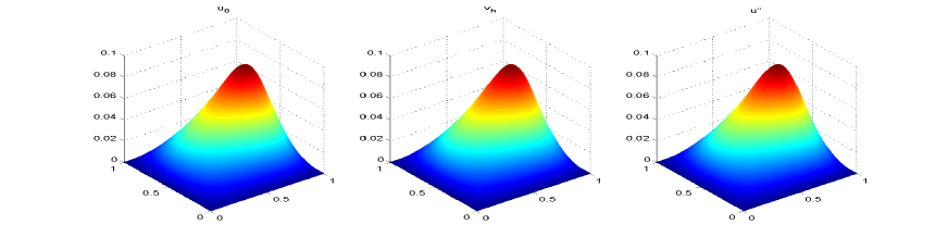
Figure 2. Solutions in D and $\delta=0.05$. Left: the homogenized solution $u_{0}$; Middle: the solution of the concurrent method; Right: the solution of Problem (1.1).

We plot the zoomed-in solutions inside the defect domain $K_{0}$ in Figure 3, it seems the hybrid solution approximates the original solution very well because it captures the oscillation of the microstructures inside $K_{0}$.

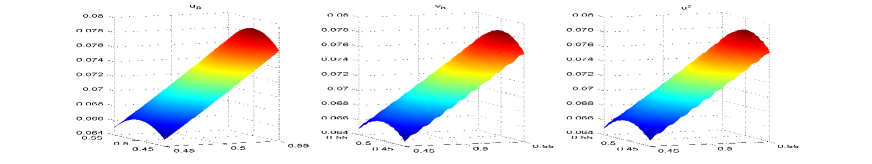
Figure 3. Solutions inside the defect domain $K_{0}$ and $\delta=0.05$. Left: the homogenized solution $u_{0}$; Middle: the solution of the concurrent method; Right: the solution of Problem (1.1).

Next we plot the zoomed-in solutions in $D\backslash K$ in Figure 4, i.e., outsie the defect domain $K_{0}$, it seems that the hybrid solution approximates the homogenized solution very well because it is as smooth as the homogenized solution, while there is oscillation in $u^{\varepsilon}$.

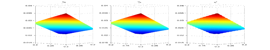
Figure 4. Solution in a subdomain of $D/K$ and $\delta=0.05$. Left: the homogenized solution $u_{0}$; Middle: the solution of the concurrent method; Right: the solution of Problem (1.1).

The localized error $\|u^{\varepsilon}-v_{h}\|_{H^{1}(K_{0})}$ is shown in Figure 5(a) for both the smooth and nonsmooth transition functions. Here the nonsmooth transition function is the characteristic function of $K_{0}$. The results show first that the parameter $\delta$ has little influence on the local energy error, and secondly the result obtained by the nonsmooth transition function is less accurate.

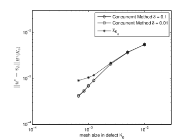
(a)

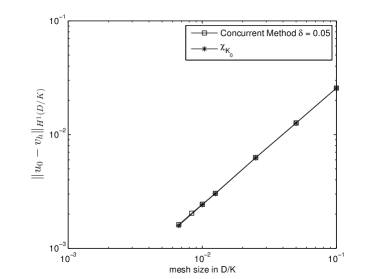
(b)

Figure 5. (a) Localized H¹ error with respective to the mesh size inside the defect domain $K_{0}$. (b) Error between the hybrid solution and the homogenized solution outside $K$.

Finally, we plot the error $\|u_{0}-v_{h}\|_{H^{1}(D\backslash K)}$ in Figure 5(b) for both the smooth and nonsmooth transition functions. For fixed $L$, this quantity decreases as the mesh outside $K$ is refined. It seems that the smoothness of the transition function has little effect on the accuracy of the homogenized solution, which is consistent with the theoretical results.

The results in Table 1 show the convergence rate of the hybrid solution to the homogenized solution. It is optimal in the sense that the solution of the hybrid problem converges to the homogenized solution with first order in the energy norm, and it converges with second order in the $L^{2}$ norm. This seems consistent with the theoretical estimates (3.4) and (3.5), because

$$\|\nabla(u_{0}-v_{h})\|_{L^{2}(D)}\leq C\left(h+L\left\lvert\ln L\right\rvert^{1/2}\right),\quad\|u_{0}-v_{h}\|_{L^{2}(D)}\leq C\left(h^{2}+L^{2}\left\lvert\ln L\right\rvert\right).$$

When $L\simeq h$, the convergence rate is of first order with respect to the energy norm, while the mesh size is smaller than $L$, the dominant term in the error bound is $L\left\lvert\ln L\right\rvert^{1/2}$, the convergence rate deteriorates a little bit, which is clear from the last line of Table 1. The same scenario applies to the $L^{2}$ error estimate.

Table 1. Error between the hybrid solution and the homogenized solution outside $K$.

h	$\|u_{0}-v_{h}\|_{L^{2}(D\backslash K)}$	order	$\|u_{0}-v_{h}\|_{H^{1}(D\backslash K)}$	order
1/10	9.04E-04		2.56E-02
1/20	2.47E-04	1.87	1.26E-02	1.02
1/40	7.96E-05	1.64	6.28E-03	1.01
1/80	3.41E-05	1.22	3.04E-03	1.04
1/160	2.47E-05	0.47	1.61E-03	0.92

4.2. An example without scale separation in the defect domain

The setup for the second example is the same with the first one except that the coefficient is replaced by $a^{\varepsilon}=\chi_{K_{0}}\tilde{a}+(1-\chi_{K_{0}})\tilde{a}^{\varepsilon}$, where

$$\tilde{a}(x)=3+\frac{1}{7}\sum_{j=0}^{4}\sum_{i=0}^{j}\frac{1}{j+1}\cos\left(\left\lfloor 8(ix_{2}-\frac{x_{1}}{i+1})\right\rfloor+\left\lfloor 150ix_{1}\right\rfloor+\left\lfloor 150x_{2}\right\rfloor\right),$$

and

$$\tilde{a}^{\varepsilon}(x)=\left(2.1+\cos(2\pi x_{1}/\varepsilon)\cos(2\pi x_{2}/\varepsilon)+\sin(4x_{1}^{2}x_{2}^{2})\right)I.$$

The above coefficient is taken from [Abdulle:15], which has no clear scale inside $K_{0}$; while it is locally periodic outside $K_{0}$. We plot the coefficient $a^{\varepsilon}$ in Figure 6 with $\varepsilon=0.1$.

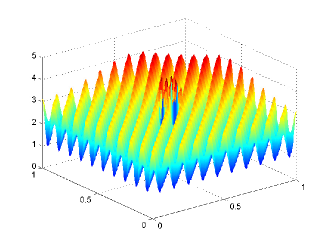
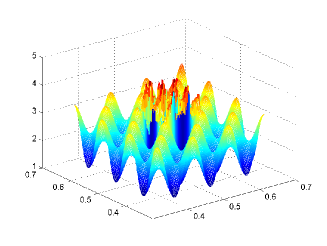
Figure 6. Coefficient $a^{\varepsilon}$ with $\varepsilon=0.1$. The right one is the zoomed-in plot near the defect.

We let $\varepsilon=0.0063$ for the sake of comparison with those in [Abdulle:15] and compute $u^{\varepsilon}$ over a uniform mesh with mesh size $3.33e-4$. By Corollary 2.2 and the identity (2.6), the effective matrix $\mathcal{A}=\chi_{K_{0}}\widetilde{a}+(1-\chi_{K_{0}})\widetilde{A}$ and the approximating effective matrix $\mathcal{A}_{h}=\chi_{K_{0}}\widetilde{a}+(1-\chi_{K_{0}})\widetilde{A}_{h}$, where $\widetilde{A}_{h}$ is an approximation of the effective matrix associated with $\widetilde{a}^{\varepsilon}$ through a fast solver based on the discrete least-squares reconstruction in the framework of HMM (see [LiMingTang:2012] and [HuangLiMing:2016] for details of such fast algorithm). We reconstruct $\widetilde{A}_{h}$ to high accuracy so that the reconstruction error is negligible. The homogenized solution $u_{0}$ is computed by solving Problem (1.2) with $\mathcal{A}$, which has also been used in solving the hybrid problem (1.5), i.e.,

$$b_{h}^{\varepsilon} =\rho\chi_{K_{0}}\widetilde{a}+\rho(1-\chi_{K_{0}})\widetilde{a}^{\varepsilon}+(1-\rho)\chi_{K_{0}}\widetilde{a}+(1-\rho)(1-\chi_{K_{0}})\widetilde{A}_{h}$$

$$=\chi_{K_{0}}\widetilde{a}+(1-\chi_{K_{0}})\left(\rho\widetilde{a}^{\varepsilon}+(1-\rho)\widetilde{A}_{h}\right).$$

We solve Problem (1.5) over a non-uniform mesh as in Figure 1, and plot $u^{\varepsilon},v_{h}$ and $u_{0}$ and the zoomed-in solution in Figure 7. The difference among them are small because there is no explicit scale inside the defect domain $K_{0}$.

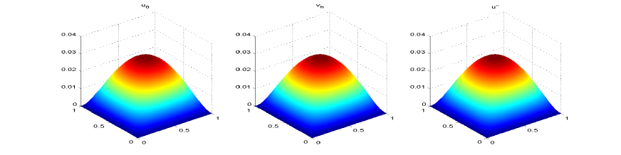
(a) Solutions in D

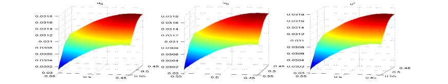
(b) Solutions in $K_{0}$.

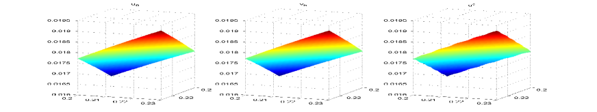
(c) Solutions in a subdomain of $D/K$.

Figure 7. The solution of hybrid method with $\delta=0.05$ in the simulation.

We plot the localized $H^{1}$ error in Figure 8(a). It seems the hybrid method converges slightly faster than the direct method, and the parameter $\delta$ has no significant effect on the results.

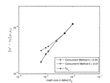
(a)

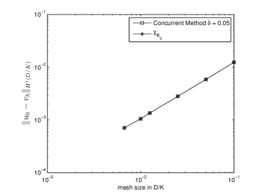
(b)

Figure 8. (a) Localized H¹ error with respective to the mesh size inside $K$ with different $\delta$. (b) Error between the hybrid solution and the homogenized solution outside $K$.

Next we plot the error outside $K$ in Figure 8(b). The results in Table 2 shows that the convergence rate of the hybrid solution to the homogenized solution is optimal with respect to both the energy norm and the $L^{2}$ norm.

Table 2. Error between the hybrid solution and the homogenized solution outside $K$.

h	$\|u_{0}-v_{h}\|_{L^{2}(D\backslash K)}$	order	$\|u_{0}-v_{h}\|_{H^{1}(D\backslash K)}$	order
1/10	3.93E-04		1.24E-02
1/20	8.92E-05	2.14	5.86E-03	1.08
1/40	2.06E-05	2.11	2.81E-03	1.06
1/80	4.92E-06	2.07	1.35E-03	1.06
1/160	1.45E-06	1.76	7.05E-04	0.94

4.3. Comparison with the global-local approach

In this part, we compare the present method with the global-local method [OdenVemaganti:2000]. The local region is $\Omega_{\eta}=(0.5,0.5)+(-L-\eta,L+\eta)^{2}$ for a positive parameter $\eta$. The recovered solution is denoted by $\widetilde{u}^{\epsilon}$. The results for Example 4.1 and Example 4.2 are plotted in Figure 9 and Figure 10, respectively. The results in both figures show that the concurrent approach yields comparable results with those obtained by the global-local approach, and the concurrent approach being slightly more accurate. Moreover, it seems the parameter $\eta$ has little effect on the accuracy of the global-local method.

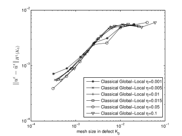
(a)

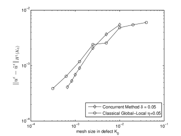
(b)

Figure 9. (a)Localized H¹ error inside $K_{0}$ for Example 4.1 by the global-local method with different $\eta$. (b) Comparison of the localized H¹ error inside $K_{0}$ for Example 4.1 with the global-local approach and the concurrent method.

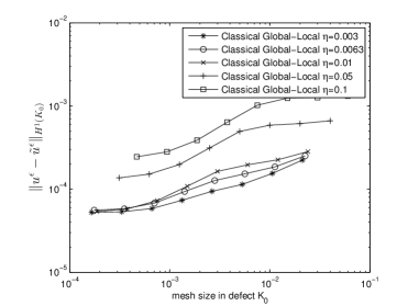
(a)

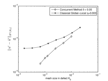
(b)

Figure 10. (a) Localized H¹ error inside $K_{0}$ for Example 4.2 by the global-local method with different $\eta$. (b) Comparison of the localized H¹ error inside $K_{0}$ for Example 4.2 with the global-local approach and the concurrent method.

5. Conclusion

We propose a new hybrid method that retrieves the global macroscopic information and resolves the local events simultaneously. The efficiency and accuracy of the proposed method have been demonstrated for problems with or without scale separation. The rate of convergence has been established when the coefficient is either periodic or almost-periodic.

For possible future directions, the formulation of the method can be naturally extended to treat problems with finite number of localized defects, the random coefficients and also time-dependent problems. It is also interesting to study the case when the local mesh inside the defect domain is not body-fitted, which can be done with the aid of the existing methods for elliptic interface problem; See e.g., [Gunzman:2016]. We shall leave these for further exploration.

Appendix A Example

To better appreciate the estimates (3.4) and (3.5), which are crucial in our analysis, let us consider a one-dimensional problem

$$\left\{\begin{aligned} &-\left(a^{\,\varepsilon}(x)u^{\prime}(x)\right)^{\prime}=0,\quad x\in(0,1),\\ &u(0)=0,\quad a^{\,\varepsilon}(1)u^{\prime}(1)=1,\end{aligned}\right.$$

where $a^{\,\varepsilon}(x)=2+\sin(x/\varepsilon)$. A direct calculation gives that the effective coefficient $\mathcal{A}=\sqrt{3}$ and the solution of the homogenized problem is $u_{0}(x)=x/\mathcal{A}$.

We consider a uniform mesh given by

$$x_{0}=0<x_{1}=h<\cdots<x_{i}=ih<\cdots<x_{2N}=1,$$

where $h=1/(2N)$. The finite element space $X_{h}$ is simply the piecewise linear element associated with the above mesh with zero boundary condition at $x=0$.

Case $h\gg\varepsilon$. We firstly consider the case that $h\gg\varepsilon$, while the precise relation between $h$ and $\varepsilon$ will be made clear below. Denote $v_{h}(x_{j})=v_{j}$ and the interval $I_{j}=(x_{j-1},x_{j})$, the mean of the coefficients $b^{\,\varepsilon}$ over each $I_{j}$ is denoted by $b_{j}={\int\negthickspace\negthickspace\negthickspace\negthinspace-}_{I_{j}}b^{\,\varepsilon}(x)\,\mathrm{d}x$.

We define the transition function $\rho$ as a piecewise linear function that is supported in $(-2L,2L)$, where $L$ is a fixed number with $0<L<1/4$. Without loss of generality, we assume that $L=Mh$ with $M$ an integer. In particular,

$$\rho(x)=\left\{\begin{aligned} 0&\quad 0\leq x\leq x_{N-2M},\\ \dfrac{x-x_{N-2M}}{L}&\quad x_{N-2K}\leq x\leq x_{N-M},\\ 1&\quad x_{N-M}\leq x\leq x_{N+M},\\ \dfrac{x_{N+2M}-x}{L}&\quad x_{N+M}\leq x\leq x_{N+2M},\\ 0&\quad x_{N+2M}\leq x\leq x_{2N}=1.\end{aligned}\right.$$

By construction, we get the size of the support of $\rho$ is $\left\lvert K\right\rvert=4L$.

We easily obtain the linear system for $\{v_{j}\}_{j=1}^{2N}$ as

$$\left\{\begin{aligned} -b_{j}v_{j-1}+(b_{j}+b_{j+1})v_{j}-b_{j+1}v_{j+1}&=0,\quad j=1,\cdots,2N-1,\\ -b_{2N}v_{2N-1}+b_{2N}v_{2N}&=h.\end{aligned}\right.$$

Define $c_{j}{:}=(v_{j}-v_{j-1})b_{j}/h$, we rewrite the above equation as

$$c_{j}-c_{j-1}=0,\quad j=1,\cdots,2N-1,\qquad c_{2N}=1.$$

Hence $c_{j}=1$ for $j=1,\cdots,2N$, and the above linear system reduces to

$$(v_{j}-v_{j-1})b_{j}=h.$$

Using $v_{0}=0$, we obtain

(A.1) $$v_{j}=h\sum_{i=1}^{j}\dfrac{1}{b_{i}}.$$

Observing that $v_{h}(x)=u_{0}(x)$ for $x\in[0,x_{N-2M}]$ because they are linear functions that coincide at all the nodal points $x_{i}$ for $i=0,\cdots,N-2M$.

For $x\in I_{N-2M+j+1}$, we obtain

$$u_{0}(x)-v_{h}(x)=h\sum_{i=1}^{j}\left(\dfrac{1}{\mathcal{A}}-\dfrac{1}{b_{N-2M+i}}\right)+(x-x_{N-2M+j})\left(\dfrac{1}{\mathcal{A}}-\dfrac{1}{b_{N-2M+j+1}}\right).$$

Define $S_{j}{:}=h\sum_{i=1}^{j}\left(\dfrac{1}{\mathcal{A}}-\dfrac{1}{b_{N-2M+i}}\right)$, we rewrite the above equation as

(A.2) $$u_{0}(x)-v_{h}(x)=\dfrac{x_{N-2M+j+1}-x}{h}S_{j}+\dfrac{x-x_{N-2M+j+1}}{h}S_{j+1},$$

which immediately yields

(A.3) $$\int_{x_{N-2M}}^{x_{N-M}}\left\lvert u_{0}^{\prime}(x)-v_{h}^{\prime}(x)\right\rvert^{2}\,\mathrm{d}x =h\sum_{j=1}^{M}\left\lvert\dfrac{1}{\mathcal{A}}-\dfrac{1}{b_{N-2M+j}}\right\rvert^{2}$$

$$\geq\dfrac{h}{27}\sum_{j=1}^{M}\left\lvert\mathcal{A}-b_{N-2M+j}\right\rvert^{2}.$$

This is the starting point of later derivation. A direct calculation gives

$$b_{N-2M+j}-\mathcal{A} ={\int\negthickspace\negthickspace\negthickspace\negthinspace-}_{I_{N-2M+j}}\rho(x)(a^{\varepsilon}(x)-\mathcal{A})\,\mathrm{d}x$$

$$=\dfrac{2-\mathcal{A}}{2}\bigl{(}\rho(x_{N-2M+j-1})+\rho(x_{N-2M+j})\bigr{)}+{\int\negthickspace\negthickspace\negthickspace\negthinspace-}_{I_{N-2M+j}}\sin\dfrac{x}{\varepsilon}\,\mathrm{d}x$$

$$=\dfrac{(2-\mathcal{A})h}{2L}(2j-1)+{\int\negthickspace\negthickspace\negthickspace\negthinspace-}_{I_{N-2M+j}}\sin\dfrac{x}{\varepsilon}\,\mathrm{d}x,$$

and an integration by parts yields

$${\int\negthickspace\negthickspace\negthickspace\negthinspace-}_{I_{N-2M+j}}\sin\dfrac{x}{\varepsilon}\,\mathrm{d}x =\dfrac{2j\varepsilon}{L}\sin\dfrac{h}{2\varepsilon}\sin\dfrac{x_{N-2M+j-1/2}}{\varepsilon}$$

$$\quad-\dfrac{\varepsilon}{L}\cos\dfrac{x_{N-2M+j-1}}{\varepsilon}+\dfrac{\varepsilon^{2}}{Lh}\left(\cos\dfrac{x_{N-2M+j-1}}{\varepsilon}-\cos\dfrac{x_{N-2M+j}}{\varepsilon}\right).$$

Combining the above two equations, we obtain

(A.4) $$b_{N-2M+j}-\mathcal{A}=\dfrac{(2-\mathcal{A})h}{2L}(2j-1)+\dfrac{2j\varepsilon}{L}\sin\dfrac{h}{2\varepsilon}\sin\dfrac{x_{N-2M+j-1/2}}{\varepsilon}+\text{REM},$$

where the remainder term

$$\text{REM}{:}=-\dfrac{\varepsilon}{L}\cos\dfrac{x_{N-2M+j-1}}{\varepsilon}+\dfrac{\varepsilon^{2}}{Lh}\left(\cos\dfrac{x_{N-2M+j-1}}{\varepsilon}-\cos\dfrac{x_{N-2M+j}}{\varepsilon}\right),$$

which can be bounded as

$$\left\lvert\text{REM}\right\rvert \leq\dfrac{\varepsilon}{L}+\dfrac{2\varepsilon^{2}}{Lh}\left\lvert\sin\dfrac{h}{2\varepsilon}\right\rvert\left\lvert\cos\dfrac{x_{N-2M+j-1/2}}{\varepsilon}\right\rvert$$

$$\leq\dfrac{\varepsilon}{L}+\dfrac{2\varepsilon^{2}}{Lh}\dfrac{h}{2\varepsilon}=\dfrac{2\varepsilon}{L}.$$

Note that $\sum_{j=1}^{M}(2j-1)^{2}=M(4M^{2}-1)/3,$ and

$$\sum_{j=1}^{M}j^{2}\sin^{2}\dfrac{x_{N-2M+j-1/2}}{\varepsilon}\leq\sum_{j=1}^{M}j^{2}=\dfrac{1}{6}M(M+1)(2M+1).$$

Summing up all the above estimates and using the elementary inequality

$$(a+b+c)^{2}+b^{2}+c^{2}\geq\dfrac{a^{2}}{3}\quad\text{for any\quad}a,b,c\in\mathbb{R},$$

we have, for $M\geq 3$,

$$\sum_{j=1}^{M}\left\lvert\mathcal{A}-b_{N-2M+j}\right\rvert^{2} \geq\dfrac{1}{3}\dfrac{(2-\mathcal{A})^{2}h^{2}}{4L^{2}}\sum_{j=1}^{M}(2j-1)^{2}-\dfrac{4\varepsilon^{2}}{L^{2}}\sin^{2}\dfrac{h}{2\varepsilon}\sum_{j=1}^{M}j^{2}\sin^{2}\dfrac{x_{N-2M+j-1/2}}{\varepsilon}$$

$$\quad-\dfrac{4Mh\varepsilon^{2}}{L^{2}}$$

$$\geq\dfrac{(2-\mathcal{A})^{2}h^{2}}{36L^{2}}M(4M^{2}-1)-\dfrac{2\varepsilon^{2}}{3L^{2}}M(M+1)(2M+1)-\dfrac{4M\varepsilon^{2}}{L^{2}}$$

$$\geq\dfrac{(2-\mathcal{A})^{2}h^{2}}{36L^{2}}M(4M^{2}-1)-\dfrac{2\varepsilon^{2}}{3L^{2}}M(4M^{2}-1)$$

$$\geq\dfrac{(2-\mathcal{A})^{2}h^{2}}{72L^{2}}M(4M^{2}-1)$$

provided that $\varepsilon/h\leq(2-\mathcal{A})/(4\sqrt{3})$. Substituting the above estimate into (A.3), we obtain

$$\int_{x_{N-2M}}^{x_{N-M}}\left\lvert u_{0}^{\prime}(x)-v_{h}^{\prime}(x)\right\rvert^{2}\,\mathrm{d}x \geq\dfrac{(2-\mathcal{A})^{2}h^{3}}{1944L^{2}}M(4M^{2}-1)$$

$$\geq\dfrac{(2-\mathcal{A})^{2}h^{3}}{648L^{2}}M^{3}=\dfrac{(2-\mathcal{A})^{2}}{648}L.$$

This implies

$$\|u_{0}^{\prime}-v_{h}^{\prime}\|_{L^{2}(1/2-2L,1/2-L)}\geq\dfrac{2-\mathcal{A}}{18\sqrt{2}}L^{1/2}=\dfrac{2-\mathcal{A}}{36\sqrt{2}}\left\lvert K\right\rvert^{1/2}.$$

This shows that the factor $\left\lvert K\right\rvert^{1/2}$ in (3.4) is sharp. The same argument shows the size-dependence of $\left\lvert K\right\rvert$ in the estimate (3.5).

Case $h\ll\varepsilon$. We next consider the case when $h\ll\varepsilon$. In fact, we may employ coarser mesh with mesh size $H$ outside the defect region with $H\gg h$, while a finer mesh with mesh size $h$ inside the defect region. The above derivation remains true and we still have $v_{h}(x)=u_{0}(x)$ for $x\in[0,1/2-2L]$. We start from the inequality (A.3). Notice that the dominant term in the expression of $b_{N-2M+j}-\mathcal{A}$ is the oscillatory one in (A.4). Denote $\phi=2h/\varepsilon$. A direct calculation gives

$$\quad\sum_{j=1}^{M}j^{2}\sin^{2}\dfrac{x_{N-2M+j-1/2}}{\varepsilon}=\dfrac{1}{2}\sum_{j=1}^{M}j^{2}-\dfrac{1}{2}\sum_{j=1}^{M}\cos\dfrac{x_{2N-4M+2j-1}}{\varepsilon}$$

$$=\dfrac{1}{12}M(M+1)(2M+1)$$

$$\quad-\biggl{\{}\dfrac{M(M+1)}{4\sin(\phi/2)}\sin[(N-M)\phi]+\dfrac{M+1}{4\sin^{2}\phi/2}\cos[(N-M)\phi]\cos\dfrac{\phi}{2}$$

$$\qquad\quad-\dfrac{\cos[(N-3M/2-1)\phi]\cos\dfrac{\phi}{2}\sin\dfrac{M+1}{2}\phi}{4\sin^{3}(\phi/2)}\biggr{\}}.$$

We assume that

(A.5) $$\sin\dfrac{\phi}{2}\geq\dfrac{5}{M}.$$

Denote the terms in the curled bracket by $I$. Given (A.5), using the elementary inequalities $2x/\pi\leq\sin x\leq x$ for $x\in[0,\pi/2]$, we bound $I$ as

$$\left\lvert I\right\rvert \leq\dfrac{(M+1)M}{4\sin(\phi/2)}+\dfrac{M+1}{4\sin^{2}(\phi/2)}+\dfrac{(M+1)\phi/2}{4\sin^{3}(\phi/2)}$$

$$\leq\dfrac{(M+1)M}{4\sin(\phi/2)}+\dfrac{M+1}{4\sin^{2}(\phi/2)}+\dfrac{(M+1)\pi}{8\sin^{2}(\phi/2)}$$

$$\leq\dfrac{M^{2}(M+1)}{12},$$

which immediately yields

$$\sum_{j=1}^{M}j^{2}\sin^{2}\dfrac{x_{N-2M+j-1/2}}{\varepsilon}\geq\dfrac{M^{3}}{12}.$$

This implies

$$\dfrac{4\varepsilon^{2}}{L^{2}}\sin^{2}\dfrac{h}{2\varepsilon}\sum_{j=1}^{M}j^{2}\sin^{2}\dfrac{x_{N-2M+j-1/2}}{\varepsilon}\geq\dfrac{4\varepsilon^{2}}{L^{2}}\left(\dfrac{2}{\pi}\dfrac{h}{2\varepsilon}\right)^{2}\dfrac{M^{3}}{12}=\dfrac{M}{3\pi^{2}}.$$

Note also

$$\dfrac{(2-\mathcal{A})^{2}h^{2}}{4L^{2}}\sum_{j=1}^{M}(2j-1)^{2}\leq\dfrac{(2-\mathcal{A})^{2}}{3}M.$$

Combining the above two estimates, we obtain

$$\sum_{j=1}^{M}\left\lvert\mathcal{A}-b_{N-2M+j}\right\rvert^{2} \geq\dfrac{1}{2}\sum_{j=1}^{M}\left(\dfrac{2\varepsilon}{L}\sin\dfrac{h}{2\varepsilon}j\sin\dfrac{x_{N-2M+j-1/2}}{\varepsilon}+\dfrac{(2-\mathcal{A})h}{2L}(2j-1)\right)^{2}$$

$$\quad-\dfrac{4M\varepsilon^{2}}{L^{2}}$$

$$\geq\left(\dfrac{1}{6}\left(1/\pi+\mathcal{A}-2\right)^{2}-\dfrac{4\varepsilon^{2}}{L^{2}}\right)M>0$$

provided that

$$h>\dfrac{\sqrt{6}\varepsilon}{(1/\pi+\mathcal{A}-2)M}.$$

This condition suffices for the validity of (A.5), which is satisfied under a weaker condition $h>{5\pi\varepsilon}/(2M).$

Substituting the above estimate into (A.3), we may find that there exists $C$ depending only on $\mathcal{A}$ such that

$$\|u_{0}^{\prime}-v_{h}^{\prime}\|_{L^{2}(1/2-2L,1/2-L)}\geq CL^{1/2}=\dfrac{C}{2}\left\lvert K\right\rvert^{1/2}.$$

This proves that the factor $\left\lvert K\right\rvert^{1/2}$ is sharp for (3.4). The same argument shows the size-dependence of $\left\lvert K\right\rvert$ in the estimate (3.5).