A Computationally Efficient Approach for Calculating Galaxy Two-Point Correlations

Abstract

We developed a modification to the calculation of the two-point correlation function commonly used in the analysis of large scale structure in cosmology. An estimator of the two-point correlation function is constructed by contrasting the observed distribution of galaxies with that of a uniformly populated random catalog. Using the assumption that the distribution of random galaxies in redshift is independent of angular position allows us to replace pairwise combinatorics with fast integration over probability maps. The new method significantly reduces the computation time while simultaneously increasing the precision of the calculation. It also allows to introduce cosmological parameters only at the last and least computationally expensive stage, which is helpful when exploring various choices for these parameters.

1 Introduction

The two-point spatial correlation function (2pcf) is a key tool used in astrophysics for the study of large scale structure (LSS). Given an object such as a galaxy, the number of other galaxies within a volume element $\Delta V$ at a distance $s$ from the first galaxy is

$$\Delta N=\overline{n}(1+\xi(s))\Delta V,$$ (1)

where $\overline{n}$ is the mean number density and $\xi(s)$ is the two-point correlation function characterizing the deviation from the uniform distribution in separation between galaxies (Peebles, 1973).

The correlation function $\xi(s)$ and its Fourier transform, the galaxy power spectrum $\mathcal{P}(k)$, have been used to describe the distribution of matter in galaxy surveys (Yu & Peebles, 1969; Peebles & Hauser, 1974; Groth & Peebles, 1977; Feldman et al., 1994). During the past decade $\xi(s)$ has become a popular tool for the reconstruction of the clustering signal known as baryon acoustic oscillations, or BAO (Eisenstein et al., 2005). The BAO signal is the signature of the density differences that arose in the early universe before the thermal decoupling of photons and baryons (Sunyaev & Zeldovich, 1970; Peebles & Yu, 1970). It is detectable today as a characteristic peak in the galaxy spatial correlation function at roughly $s=110h^{-1}$ Mpc, where $h$ defines the Hubble parameter $H_{0}=100h$ km s^-1 Mpc^-1.

Given a spectroscopic survey containing the 3D coordinates of each galaxy, there exist several possible ways to estimate $\xi(s)$. The most popular estimator is due to Landy & Szalay (1993), which is constructed by combining pairs of galaxies from a catalog of observed objects $D$ (“data”) and a randomly generated catalog $R$ with galaxies distributed uniformly over the fiducial volume of the survey but using the same selection function as the data. The Landy-Szalay (LS) estimator is

$$\hat{\xi}(s)=\frac{DD(s)-2DR(s)+RR(s)}{RR(s)},$$ (2)

where $DD$, $RR$, and $DR$ are the normalized distributions of the pairwise combinations of galaxies from the data and random catalogs (plus cross terms) at a given distance $s$ from each other.

There exist many 2pcf estimators other than the LS estimator, and they have different advantages and limitations. However, all commonly known estimators are functions of $DR$ and/or $RR$ distributions (see Hamilton (1993); Kerscher et al. (2000); Vargas-Magana et al. (2013)) and therefore depend on the random catalog $R$. To limit statistical fluctuations in $\hat{\xi}(s)$, it is typical to generate random catalogs with one to two orders of magnitude more galaxies than the survey under investigation. Unfortunately, the “brute-force” computation of $\hat{\xi}(s)$, in which all possible pair combinations are counted, is an $\mathcal{O}(N_{R}^{2})$ calculation due to $RR$, where $N_{R}$ is the number of galaxies in the random catalog $R$; this results in a trade-off between statistical uncertainties and computation time. This trade-off has consequences beyond reducing uncertainties. For example, researchers often simulate a variety of cosmological parameters when studying the LSS, but the computational overhead required to calculate $\hat{\xi}(s)$ may limit the number and type of possible analyses that can be carried out. The overhead also increases the effort needed to compute the covariance of the 2pcf as well as the effect of different sources of systematic uncertainties.

In this paper, we suggest a method which substantially reduces the time needed to compute $RR$ and $DR$ and hence is applicable to any estimator $\hat{\xi(s)}$. Moreover, the computationally intensive part of the calculation is independent of the choice of cosmological parameters, allowing exploring a larger parameter space. The method is based on the assumption that the probability for a galaxy to be observed at a particular location in the random catalog can be factorized into separate angular and redshift components. This assumption is frequently made in the analysis of large scale structures and it allows us to replace pairwise combinatorics in the calculations of $RR$ and $DR$ with fast integration over probability maps. We find that the estimation of $\hat{\xi}(s)$ significantly speeds up with respect to the brute-force calculation. In practical terms, this means an estimate of $\hat{\xi}(s)$ which is typically carried out on large computing clusters can be performed on a modern notebook computer.

The paper is structured as follows. In Section 2 we describe the mathematical justification of the method. In Section 3 we describe the resulting algorithm used to compute $\hat{\xi}(s)$ in detail. The performance of the algorithm is studied in Section 4 using mock catalogs and spectroscopic data from the CMASS portion of the Sloan Digital Sky Survey (SDSS) DR9 catalog (Ross et al., 2012; Sanchez et al., 2012; Anderson et al., 2013; Percival et al., 2014). We then conclude in Section 5.

2 Mathematical proof

2.1 Random-random distribution

The 3D position of any galaxy $\vec{r}$ is described by its right ascension $\alpha$, declination $\delta$, and its redshift $z$. Based on this information the cosmological distances are calculated given a set of cosmological parameters: $\Omega_{M}$ - the present day relative matter density of the universe, $\Omega_{k}$ - the measure of the curvature of space, and $\Omega_{\Lambda}$ - the relative density due to the cosmological constant. The comoving radial distance $r(z)$ is calculated from the observed redshift $z$ as

$$r(z)=D_{H}I(z),\\$$ (3)

where

$$D_{H}=c/H_{0}\\$$ (4)

is the Hubble distance, $c$ is the speed of light and $I(z)$ is calculated as:

$$I(z)=\int_{0}^{z}\mathrm{d}z^{\prime}\,\left(\Omega_{M}(1+z^{\prime})^{3}+\Omega_{k}(1+z^{\prime})^{2}+\Omega_{\Lambda}\right)^{-1/2}.$$ (5)

The transverse distance $t(z)$ is calculated as:

$$t(z)=\begin{cases}D_{H}/\sqrt{\Omega_{k}}\ \sinh\big{(}\sqrt{\Omega_{k}}I(z)\big{)},\text{for }\Omega_{k}>0\\ r(z),\text{for }\Omega_{k}=0\\ D_{H}/\sqrt{|\Omega_{k}|}\ \sin\big{(}\sqrt{|\Omega_{k}|}I(z)\big{)},\text{for }\Omega_{k}<0\\ \end{cases}$$ (6)

As suggested by current cosmological constraints (see e.g. Aubourg et al. (2015); Ade et al. (2016)), $\Omega_{k}$ is small and thus eq. 6 can be approximated by

$$t(z)=r(z)\Big{(}1+\frac{\Omega_{k}}{6}\big{(}I(z)\big{)}^{2}\Big{)}.\\$$ (7)

The angular separation $\theta_{12}$ between points $1$ and $2$ given their right ascension $\alpha$, declination $\delta$ is calculated as

$$\theta_{12}=\cos^{-1}\big{(}\cos{\delta_{1}}\cos{\delta_{2}}\cos{(\alpha_{1}-\alpha_{2})}+\sin{\delta_{1}}\sin{\delta_{2}}\big{)}.$$ (8)

The distance $s_{12}$ between these two points (illustrated in Fig. 1) is approximated by:

$$s_{12}=\sqrt{\sigma_{12}^{2}+\pi_{12}^{2}},$$ (9)

where $\sigma_{12}$ and $\pi_{12}$, the distances transverse and parallel to the line of sight (LOS) respectively, are defined as:

$$\sigma_{12}=(t_{1}+t_{2})\sin{\frac{\theta_{12}}{2}},$$ (10)

$$\pi_{12}=\left|r_{1}-r_{2}\right|\cos{\frac{\theta_{12}}{2}}.$$ (11)

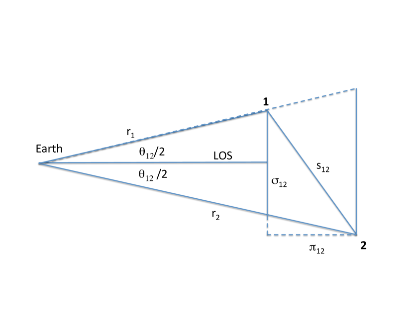
Figure 1: Calculation of the distance between points $1$ and $2$ given their comoving distances from the Earth $r_{1}$ and $r_{2}$ and their angular separation $\theta_{12}$.

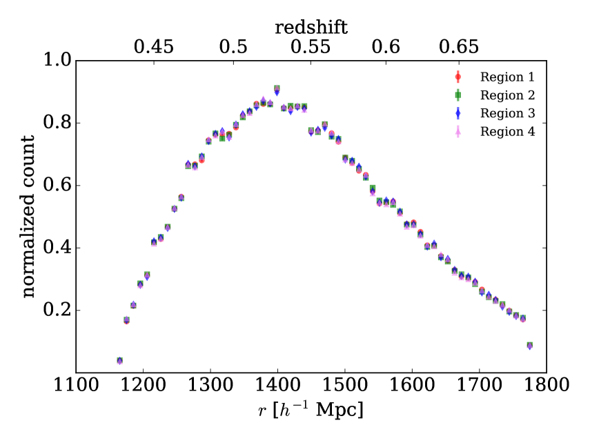
Figure 2: Distribution of galaxies over redshift and comoving distance $r$, calculated using cosmological parameters defined in Section 4, in four widely separated regions of the Northern sky based on the SDSS-III DR9 random catalog. Regions are defined by the following selection criteria: region 1 ($-4<\delta<8^{o}$, $125<\alpha<250^{o}$), region 2 ($8<\delta<57^{o}$, $108<\alpha<135^{o}$), region 3 ($25<\delta<50^{o}$, $135<\alpha<225^{o}$), region 4 ($8<\delta<40^{o}$, $225<\alpha<265^{o}$).

Since random catalogs are typically generated by uniformly populating the fiducial volume of the survey, the galaxy distribution over $z$, and thus over $r$, is factorizable from the angular distribution. In other words, any angular region of the sky has the same distribution of galaxies in $z$ (see Ross et al. (2012) and Fig. 2). This means that the expected count of random galaxies, $R(\vec{r})$, can be factorized into the product of the expected count $R_{\text{ang}}(\alpha,\delta)$ at a given angular position and a redshift probability density function (PDF) $P_{z}(z)$:

$$R(\vec{r})=R_{\text{ang}}(\alpha,\delta)P_{z}(z).$$ (12)

$R(\vec{r})$ evaluated this way has smaller statistical uncertainty since the precision of $R_{\text{ang}}(\alpha,\delta)$ depends on the number of points in the 2D angular cell, and the precision of $P_{z}(z)$ depends on the number of points in the 1D range in $z$. In contrast, the statistical precision without the factorizability assumption is determined by the number of points in a 3D cell $(z,\alpha,\delta)$. We will show in Section 4 that the uncertainties in $\hat{\xi}(s)$ evaluated using the suggested method are indeed smaller.

The expected count of random-random galaxy pairs separated by a distance $s$ can be expressed as:

$$RR(s)=\frac{1}{2}\int\mathrm{d}\Omega_{1}\mathrm{d}z_{1}\mathrm{d}\Omega_{2}\mathrm{d}z_{2}\,R_{\text{ang}}(\alpha_{1},\delta_{1})\,P_{z}(z_{1})\\ \hskip 86.72377pt\times R_{\text{ang}}(\alpha_{2},\delta_{2})\,P_{z}(z_{2})\,\delta(s-s_{12}),\\$$ (13)

where $\Omega$ represents a solid angle (and $\mathrm{d}\Omega=\cos{\delta}\,\mathrm{d}\delta\,\mathrm{d}\alpha$), $s_{12}$ is calculated according to eq. 9. The integral is taken over the entire fiducial volume of the random catalog $R$, and a factor of $1/2$ is introduced to account for double counting of the random-random pairs. The Dirac-$\delta$ function is introduced to ensure that the distance between two galaxies $s_{12}$ is equal to the distance of interest $s$. To isolate the angular variables, we rewrite the $\delta$ function in eq. 13 as an integral of the product of two $\delta$ functions:

$$\delta(s-s_{12})=\int\mathrm{d}\theta\,\delta\left(s-s_{12}\right)\delta(\theta-\theta_{12}).$$ (14)

Note that the second $\delta$ function is independent of the radial positions $r_{1},r_{2}$ of the galaxies, or their redshifts. Thus, $RR$ can be rewritten as

$$RR(s)=\int\mathrm{d}z_{1}\mathrm{d}z_{2}\mathrm{d}\theta\,P_{z}(z_{1})P_{z}(z_{2})\,f(\theta)\\ \times\delta\left(s-s_{12}\right),$$ (15)

where

$$f(\theta)=\frac{1}{2}\int\mathrm{d}\Omega_{1}\mathrm{d}\Omega_{2}\,R_{\text{ang}}(\alpha_{1},\delta_{1})\,R_{\text{ang}}(\alpha_{2},\delta_{2})\,\\ \times\delta(\theta-\theta_{12})$$ (16)

is the count of $RR$ galaxy pairs whose angular separation is $\theta$.

The count of random galaxy pairs is constructed in two steps:

1. histogramming, where we construct the distribution $f(\theta)$ over angular separation using the count of random galaxies $R_{\text{ang}}(\alpha,\delta)$ according to eq. 16,

2. integration, where we convolve the angular distribution with the redshift PDFs $P_{z}(z_{1})$ and $P_{z}(z_{2})$ to obtain the distribution of random pairs over $s$.

Note that only the second step depends on the choice of cosmological parameters.

2.2 Data-random and data-data distributions

Unlike in the random catalog, in the data catalog the distribution of galaxies over $z$ cannot be factorized from their angular distribution. Thus, the count distribution over the opening angle between galaxies in the data and random catalogs is also a function of $z_{1}$, the position of the data galaxy:

$$g(\theta,z_{1})=\int\mathrm{d}\Omega_{1}\mathrm{d}\Omega_{2}\,D(z_{1},\alpha_{1},\delta_{1})\,R_{\text{ang}}(\alpha_{2},\delta_{2})\\ \times\delta(\theta-\theta_{12}).$$ (17)

The $DR$ distribution can then be calculated as

$$DR(s)=\int\mathrm{d}z_{1}\mathrm{d}z_{2}\mathrm{d}\theta\,P_{z}(z_{2})\,g(\theta,z_{1})\\ \times\delta\left(s-s_{12}\right).$$ (18)

At the histogramming step, we construct the distribution $g(\theta,z_{1})$ according to eq. 17, keeping track of the redshift of the data galaxies $z_{1}$. At the integration step $g(\theta,z_{1})$ is convolved with the redshift PDF $P_{z}(z_{2})$ to obtain the distribution of data-random pairs over $s$ according to eq. 18.

Finally, the data-data count $DD$ is estimated using a brute-force iteration over all possible data galaxy pairs. For uniformity, the $DD$ calculation is also broken down into histogramming and integration steps. At the histogramming step the count distribution over the opening angle $u(\theta,z_{1},z_{2})$ is constructed from the pair count of data galaxies keeping track of the redshifts of both galaxies in the pair.

At the integration step, $DD(s)$ is evaluated from $u(\theta,z_{1},z_{2})$ by converting the redshifts into distances and calculating the distance between the two galaxies $s$. This breakdown does not offer any time savings in the calculation of $DD$, but it allows for the definition of the cosmological parameters only at the second step. This way the computationally intensive first step can be performed once and then the computationally fast second step is performed for each set of cosmological parameters.

2.3 Generalization of the 2pcf to anisotropic case

The discussion up to this point has dealt with only a spherically symmetric 2pcf. However, the algorithm is easily generalized to study anisotropy in the 2pcf (Davis & Peebles, 1983).

The histogramming step is identical to the isotropic case. At the integration step, we compute $RR$, $DR$ and $DD$ in two dimensions $(\sigma,\pi)$:

$$RR(\sigma,\pi)=\frac{1}{N_{RR}}\int\mathrm{d}z_{1}\mathrm{d}z_{2}d\theta\,P_{z}(z_{1})\,P_{z}(z_{2})\,f(\theta)\\ \times\delta(\sigma-\sigma_{12})\delta(\pi-\pi_{12}),$$ (19)

$$DR(\sigma,\pi)=\frac{1}{N_{DR}}\int\mathrm{d}z_{1}\mathrm{d}z_{2}\mathrm{d}\theta\,P_{z}(z_{2})\,g(\theta,z_{1})\\ \times\delta(\sigma-\sigma_{12})\delta(\pi-\pi_{12}),$$ (20)

where the distances transverse ($\sigma$) and parallel ($\pi$) to the LOS are computed according to eqs. 10 and 11 respectively.

The BAO signal is expected to manifest itself as an ellipse in this 2D histogram. In the isotropic case the ellipse is reduced to a circle.

3 Description of the algorithm

3.1 Weights

To data we apply the weights according to the prescription of Ross et al. (2012) to deal with the issues of close-pair corrections ($w_{\text{cp}}$), redshift-failure corrections ($w_{\text{rf}}$), systematic targeting effects ($w_{\text{sys}}$) and shot noise and cosmic variance ($w_{\text{FKP}}$) (Feldman et al., 1994) such that the total weight of a given data galaxy is:

$$w^{D}=w_{\text{FKP}}\cdot w_{\text{sys}}\cdot(w_{\text{rf}}+w_{\text{cp}}-1).$$ (21)

Each galaxy in the random catalog has a $z$-dependent weight $w^{R}(z)$, defined the same way as $w_{\text{FKP}}$ in data catalog. The algorithm can be generalized to the case where the random weights also depend on angular position and are factorizable into angular and redshift weights: $w^{R}=w^{R}(z)w^{R}(\alpha,\delta)$.

3.2 Binning

$RR$ and $DR$ are calculated using finely binned probability densities in $(\alpha,\delta)$ and $z$ defined from the existing random catalog, or based on the completeness map and the radial selection function. The choice of the bin sizes is important and is determined by the final bin size $\Delta s$ desired in $\hat{\xi}(s)$. In practice, this means that the bin sizes in $\alpha$, $\delta$ and $\theta$ must be smaller than the angle $\theta_{min}$ subtended by $\Delta s$ at the outermost radius of the data set, $R_{max}$ at least by a factor of two ($\theta_{min}=\Delta s/2/R_{max}$). The bin size in $z$ should be chosen such that the corresponding $\Delta r(z)$ be smaller than $\Delta s$ by the same factor. We note that the binning is not equal-area but for fine enough bins it does not affect the result. Some assumption about the cosmological parameters must be made for the calculation of $R_{max}$ and $r(z)$, so to be on the conservative side one should use the largest $R_{max}$ for the set of the cosmological parameters under evaluation, which typically means using the smallest value of $\Omega_{m}$. Using this algorithm with steps smaller than 1 $h^{-1}$ Mpc is possible but impractical as it results in an angular map that is too finely segmented and thus very large and noisy.

3.3 Limits

In the calculation presented in this paper, we only consider galaxy pairs separated by a distance less than a certain maximum distance scale of interest $l_{\text{max}}$. For this, the 2D angular space is divided into regions of the size $(\Delta\alpha,\Delta\delta)$, such that $\Delta\alpha=\Delta\delta=l_{\text{max}}/r_{min}$, where $r_{min}=R_{min}\cos(\delta_{max})$. Here, $R_{min}$ is the smallest radial distance of the survey for a set of cosmological parameters under consideration (typically corresponding to the largest value of $\Omega_{m}$), and $\delta_{max}$ is the maximum declination of the survey. The algorithm proceeds to calculate $f(\theta_{12})$, $g(\theta_{12},z_{1})$ and $u(\theta_{12},z_{1},z_{2})$ only within one $(\Delta\alpha,\Delta\delta)$ region and its neighbors.

3.4 Algorithm

3.4.1 Probability Density Functions

Once the binning and limits are chosen, the algorithm proceeds as follows. First, using the random catalog, we produce the count distribution $R_{\text{ang}}(\alpha,\delta)$ and PDF $P_{z}(z)$. For each galaxy, $P_{z}(z)$ is incremented by $w^{R}(z)/N_{R}$, and $R_{\text{ang}}(\alpha,\delta)$ is incremented by 1. If the catalog contains the angular dependent weight $w^{R}(\alpha,\delta)$ then $R_{\text{ang}}(\alpha,\delta)$ is incremented by that amount.

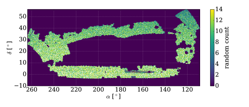
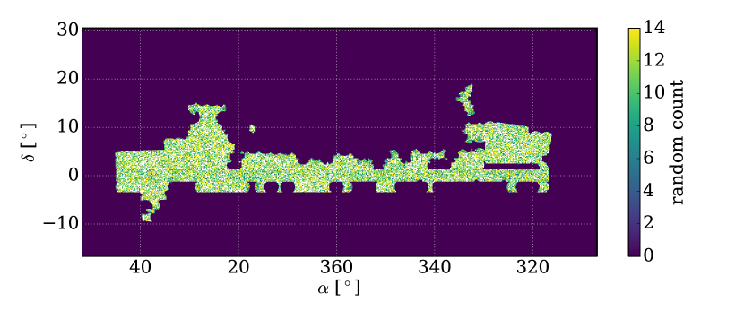
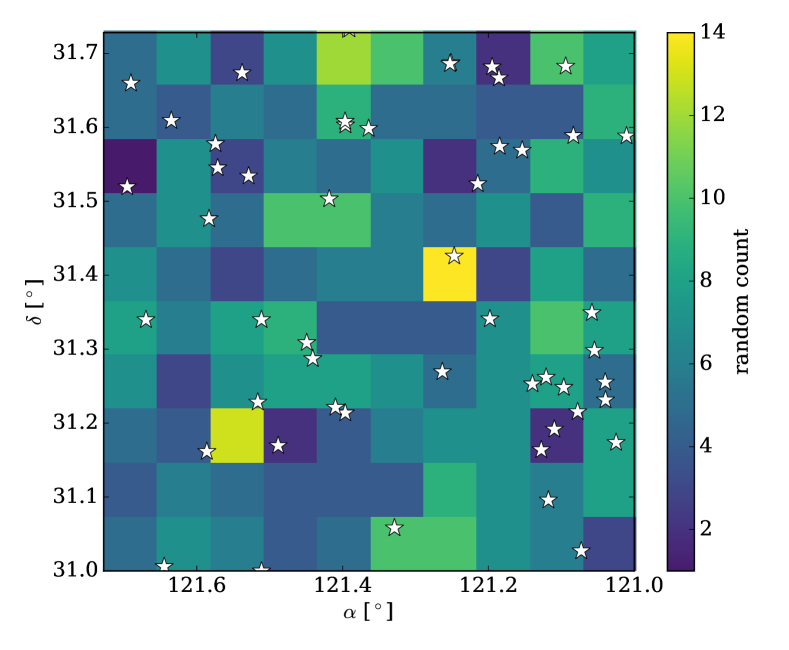
Figure 3: Top: Distribution of the DR9 random catalog in $(\alpha,\delta)$ in the northern sky. Middle: the DR9 random catalog in the southern sky. Bottom: a zoomed-in view of northern sky. The positions of galaxies observed in the DR9 survey are plotted as white stars.

This part of the algorithm is linear in the number of galaxies in random catalog and hence is very fast.

Examples of binned angular histograms are shown in Fig. 3. It is clear from the zoomed up view that the statistical fluctuations, determined by the finite size of the random catalog, are significant. However, it is important to note that these fluctuations are much smaller than the fluctuations in 3D cells with full coordinates $(z,\alpha,\delta)$, effectively used in the brute-force approach, or in any other approach that relies on 3D number density distribution. In this paper, we generate the 2D angular and 1D redshift probability maps based on an existing random catalog (published along with the observational data), but ideally these maps should be generated directly based on the tile completeness and radial selection function. This approach will create smoother probability maps and minimize the shot noise associated with the use of random catalogs.

3.4.2 Histogramming

We compute the random-random 1D binned distribution $f(\theta_{12})$ using $R_{\text{ang}}(\alpha,\delta)$. To compute binned $f(\theta_{12})$, we consider all non-repeating pairs of angular cells $(\alpha_{1},\delta_{1})$ and $(\alpha_{2},\delta_{2})$. The angle $\theta_{12}$ between the two cells is calculated from their angular positions using eq. 8 and the corresponding bin is incremented:

$$f(\theta_{12})\mathrel{+}=aR_{\text{ang}}(\alpha_{1},\delta_{1})R_{\text{ang}}(\alpha_{2},\delta_{2}),$$ (22)

where a factor is introduced such that $a=1/2$ when the two cells are identical and $a=1$ otherwise.

Then, we calculate the data-random 2D binned distribution $g(\theta_{12},z_{1})$ using galaxies from the data catalog and $R_{\text{ang}}(\alpha,\delta)$. Here, we consider every pair of a data galaxy $(z_{1},\alpha_{1},\delta_{1})$ and an angular cell $(\alpha_{2},\delta_{2})$. The angle $\theta_{12}$ between the data galaxy and the angular cell is calculated from their angular positions using eq. 8 and the corresponding 2D bin is incremented:

$$g(\theta_{12},z_{1})\mathrel{+}=w^{D}R_{\text{ang}}(\alpha_{2},\delta_{2}),$$ (23)

where $w^{D}$ is the weight of the data galaxy.

We compute the data-data 3D binned distribution $u(\theta_{12},z_{1},z_{2})$ by looping over all non-repeating pairs of galaxies. Each pair is weighted by the product of the weights of individual galaxies in the survey:

$$u(\theta_{12},z_{1},z_{2})\mathrel{+}=w^{D}_{1}\times w^{D}_{2}.$$ (24)

3.4.3 Integration

Next, we perform an integration over redshifts $z_{1}$ and $z_{2}$ and produce the distributions $RR$, $DR$ and $DD$. This is achieved in three nested loops iterating over $\theta_{12}$, $z_{1}$ and $z_{2}$. Given these three variables and choice of cosmological parameters, we compute the distance separation $s_{12}$ using eq. 9 and increment the corresponding bin of the final distributions:

$$RR(s_{12}) \mathrel{+}=f(\theta_{12})P_{z}(z_{1})P_{z}(z_{2}),$$ (25)

$$DR(s_{12}) \mathrel{+}=g(\theta_{12},z_{1})P_{z}(z_{2}),$$ (26)

$$DD(s_{12}) \mathrel{+}=u(\theta_{12},z_{1},z_{2}).$$ (27)

For the computation of the anisotropic 2pcf distances $\sigma_{12}$ and $\pi_{12}$ are computed according to eq. 10 and eq. 11 respectively.

3.4.4 Normalization

The histograms are normalized in the following way. For the unweighted calculation (all galaxies have weight $1$), the normalization constant of $RR$ is simply $N_{RR}=N_{R}(N_{R}-1)/2$. However, for the weighted calculation, the normalization constant $N_{RR}$ is:

$$N_{RR}=\sum_{i=1}^{N_{R}}\sum_{j=i+1}^{N_{R}}w^{R}_{i}w^{R}_{j}$$ (28)

where $w^{R}_{i}$ is the weight of the $i^{\text{th}}$ galaxy in the random catalog. In this specific form, the calculation is $\mathcal{O}\left(N_{R}^{2}\right)$ and requires a double loop over indices. However, it can be rewritten as:

$$N_{RR}=\frac{1}{2}\left[\left(\sum_{i=1}^{N_{R}}w^{R}_{i}\right)^{2}-\sum_{i=1}^{N_{R}}\left(w^{R}_{i}\right)^{2}\right]$$ (29)

which is now an $\mathcal{O}\left(N_{R}\right)$ calculation. The same approach can be applied when normalizing the $DD$ histogram.

For the unweighted calculation, the normalization constant of $DR$ is simply $N_{DR}=N_{D}\times N_{R}$ where $N_{D}$ is the total number of galaxies in the data catalog. For the weighted calculation, the normalization constant $N_{DR}$ is:

$$N_{DR}=\sum_{i=1}^{N_{D}}w^{D}_{i}\sum_{i=1}^{N_{R}}w^{R}_{i}$$ (30)

where $w^{D}_{i}$ is the weight of the $i^{\text{th}}$ galaxy in the data catalog. The normalization constant $N_{DR}$ only requires an $\mathcal{O}\left(N_{R}\right)$ computation and hence can be computed quickly even in the weighted calculation. Finally, the LS estimator is calculated according to eq. 2. All the other estimators can be calculated just as easily, based on $DD$, $RR$ and $DR$ distributions computed above.

4 Performance of the algorithm

4.1 Algorithm settings and Random catalog generation

The performance of the new algorithm is evaluated by calculating the runtime and the uncertainty of the LS estimator of the 2pcf. Though the method described in this paper can be applied under any cosmology, for certainty we assume a $\Lambda$CDM+GR flat cosmology with parameters consistent with those used in the analysis of the SDSS-III DR9 data set (Anderson et al., 2013), i.e. $\Omega_{M}=0.274$ and $\Omega_{\Lambda}=0.726$. In the distance calculation we set $H_{0}=100h$ km s^-1 Mpc^-1, and define the distances in units of $h^{-1}$ Mpc.

Usually, the calculations of $RR$ and $DR$ are the most computationally expensive since the size of the random catalog is typically much larger than the size of the data catalog. Therefore, we report the results of $RR$ and $DR$ for different sizes of random catalogs, while we do not change the data catalog.

To generate random catalogs of any desired size, we begin with the northern sky of the existing SDSS-III DR9 random catalog which contains $\sim$3.5M galaxies and extract the distributions $R_{\text{ang}}(\alpha,\delta)$ and $P_{z}(z)$. We then randomly generate new galaxies according to the product of these distributions. In each angular cell we generate the number of galaxies $N_{R}(\alpha,\delta)$, which is distributed according to Poisson distribution with a mean of $R_{\text{ang}}(\alpha,\delta)$. Each of these galaxies is assigned a redshift $z$, which is distributed according to $P_{z}(z)$. Weights are a function of the redshift $z$. While the new catalogs may amplify existing statistical fluctuations in the DR9 random catalog, our interest is in testing the runtime of the algorithms and estimating the variation from the mean in $\hat{\xi}(s)$ as a function of random catalog size. We find the bias in the 2pcf, defined as deviations from the true mean (which is zero), is significantly smaller than statistical uncertainties (Fig. 8). The bias is produced by shot noise in the random catalog, so if $R_{\text{ang}}(\alpha,\delta)$ and $P_{z}(z)$ are generated from the tile completeness and radial selection function it can be minimized.

4.2 Timing study

We compare the timing of the algorithm presented here against brute-force pair counting and the parallelized algorithm CUTE (Alonso, 2012). In all cases, we report runtime in CPU hours rather than elapsed wall-clock time. As in the fast algorithm, the brute-force pair count and computation with CUTE are performed using a grid scheme with a maximum distance of $l_{\text{max}}=400h^{-1}$ Mpc. Hence, the three sets of results include the same amount of statistics.

In Fig. 4, we show the runtime of the algorithms measured for the pure algorithmic parts of the executable, which are based on a C++ implementation running on modern CPUs for random catalog sizes of $N_{R}=\text{1M}$ to 50M galaxies. For this study we chose the following algorithm settings. The size of the binning in the right ascension $\alpha$, declination $\delta$ and the angular separation $\theta$ is 1 mrad, which corresponds to the transverse separation of 2.55 $h^{-1}$ Mpc at the outermost radius. The binning in $r$ corresponds to a separation of 1 $h^{-1}$ Mpc along the LOS. As expected, the runtime of our realization of the brute-force calculation as well as that of CUTE are proportional to $N_{R}^{2}$ for $RR$ and $N_{R}$ for $DR$. In contrast, the runtime of the fast algorithm plateaus around a constant value because it depends on the fiducial volume and the number of angular and radial bins, rather than the size of the random catalog $N_{R}$. The maximum runtime of the fast algorithm is reached when each bin in the $R_{\text{ang}}(\alpha,\delta)$ distribution is populated and hence is used in the calculation of $\hat{\xi}(s)$.

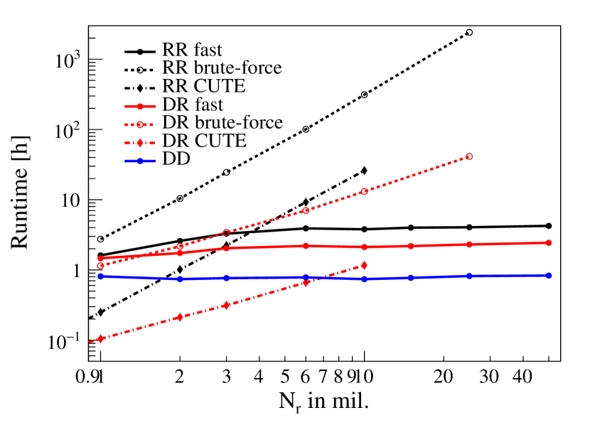
Figure 4: The total runtime (in CPU hours) of the fast, brute-force and CUTE calculations of $\hat{\xi}(s)$ as a function of the size of the random catalog.

The fits of the runtime dependence on $\Delta s$, shown in Fig. 5, include terms proportional to $\Delta s^{-1}$ and $\Delta s^{-2}$. The fits of the runtime dependence on $l_{\text{max}}$, shown in Fig. 6, include terms linear and quadratic in $l_{\text{max}}$. The numbers of bins in $\alpha$, $N_{\alpha}$ and $\delta$, $N_{\delta}$ scale inversely with the bin size $\Delta s$ in the final histogram, and linearly with the distance scale of interest $l_{\text{max}}$. The total number of the 2D angular cells is the product of $N_{\alpha}$ and $N_{\delta}$. Thus, the calculation time scales linearly with the total number of the 2D angular cells. Other fast computational techniques based on the number density rather than the actual permutation counting rely on data distribution in 3D cells (Moore et al., 2001) and thus have stronger scaling with the number of bins.

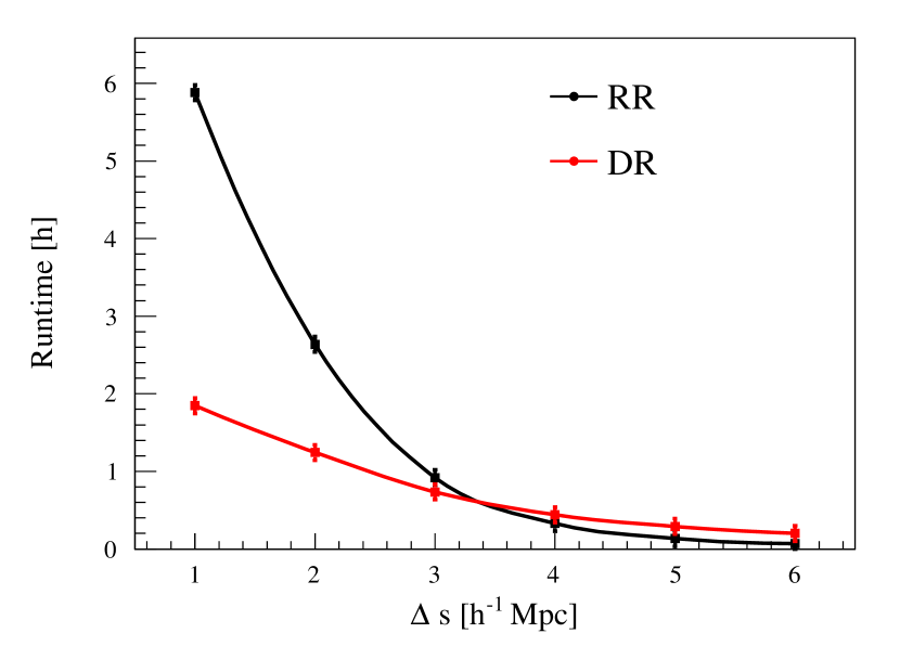
Figure 5: The total runtime (in CPU hours) of the fast calculation of the pair-wise combinations as a function of the step in $\Delta s$. In this study $l_{\text{max}}=200\,h^{-1}$ Mpc. The binning in $r$ is $\Delta s/2$. The angular binning is $\Delta s/2/R_{max}$.

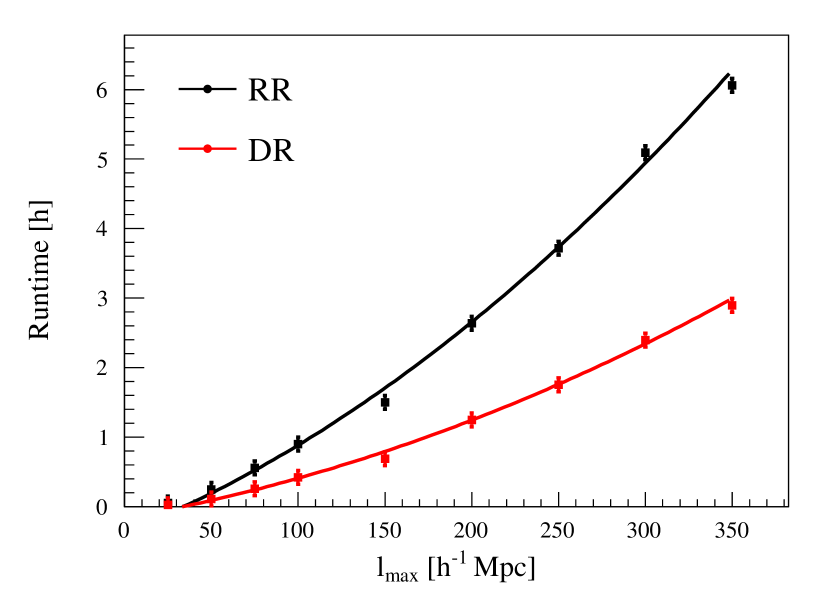
Figure 6: The total runtime (in CPU hours) of the fast calculation of the pair-wise combinations as a function of the maximum distance $l_{\text{max}}$. The binning in $r$ is $1h^{-1}$ Mpc. The angular binning is 0.56 mrad.

4.3 Algorithm precision

To check the precision of the fast algorithm we generate 20 realizations of random catalogs with 3.5M galaxies each using the procedure described above. We estimate the root mean square (RMS) of $\hat{\xi}(s)$ using the 20 random catalogs and present it in Fig. 7. Note that though the bin size used in computation is small as specified above, the result is plotted with a much larger bin size, simply for visual purposes. In both the brute-force and fast algorithms, the uncertainties in $\hat{\xi}(s)$ decrease as the size of the random catalog increases, but the uncertainties in the results based on the fast algorithm are smaller than those in the respective brute-force results, in agreement with the qualitative argument presented in Section 2.

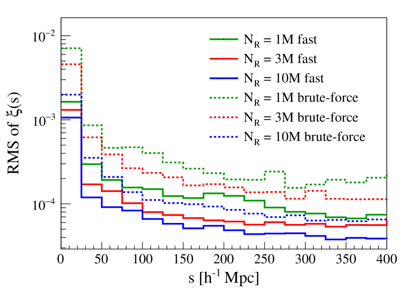
Figure 7: Uncertainties in $\hat{\xi}(s)$ as a function $s$ and the size of the random catalog. The uncertainties are calculated as the RMS of $\hat{\xi}(s)$ obtained with 20 catalogs generated for each of three catalog sizes, for both methods of computing $\hat{\xi}(s)$.

To check the fast algorithm for bias, we compute $\hat{\xi}(s)$ for 20 mock catalogs representing $D$ with 200k galaxies Poisson-distributed within the survey volume. These mock catalogs are produced using the same procedure used to generate the random catalogs. We find no significant bias; that is, the mean of $\hat{\xi}(s)$ is centered at zero as expected for a truly random distribution, and its RMS obeys a Poisson distribution (Fig. 8). Note that the Poisson error is dominated by $DD$, since the $DR$ and $RR$ are much larger and hence contribute smaller relative errors.

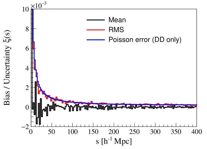
Figure 8: Mean and RMS uncertainty in $\hat{\xi}(s)$ of 20 uniformly-generated mock data sets with 200k galaxies per data set.

4.4 Performance on data with BAO signal

To demonstrate the performance of the algorithm for the anisotropic case we present the result on a mock dataset with a strong signal embedded (Fig. 9). The signal was generated by adding spatially correlated galaxy pairs on top of a uniform background. The galaxy pair separation distance is distributed according to a Gaussian of mean $105h^{-1}$ Mpc and a standard deviation of $5h^{-1}$ Mpc. To avoid biasing the $z$ distribution of galaxies in the mock sample, after signal addition some of the galaxies are removed to preserve the original distribution in $z$.

Finally, the algorithm is also applied to the SDSS-III DR9 BOSS data catalog. The results obtained from the fast algorithm and the brute-force algorithm and their difference are presented in Fig. 10. The BAO peak is clearly visible in both, and the two distributions are consistent.

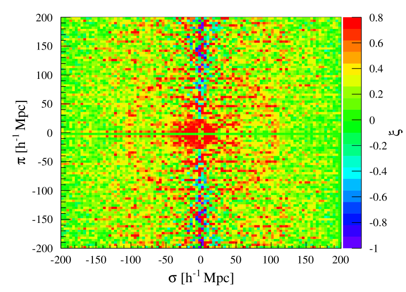
Figure 9: $\hat{\xi}(\sigma,\pi)$ based on a mock data set with embedded BAO signal with the radius of $105h^{-1}$ Mpc. The BAO signal is clearly seen as a circle in the 2D distribution.

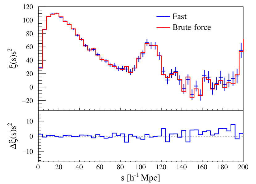
Figure 10: Top: $\hat{\xi}(s)\times s^{2}$ for SDSS-III DR9 BOSS data catalog using the fast algorithm suggested in this paper (blue) compared to brute-force calculation (red). The error bars represent Poisson uncertainties in $DD$. Bottom: the difference between the fast and brute-force estimates of $\hat{\xi}(s)\times s^{2}$.

5 Conclusion

We have presented a new computational method of the galaxy 2pcf that replaces summation over all possible galaxy pairs with a numeric integration of the probability map. The method provides a significant reduction in the calculation time and improves the precision of the calculation. Moreover, the computationally intensive histogramming part of the calculation is independent of the choice of cosmological parameters. The output of the histogramming stage is used at the fast integration stage, where the cosmological parameters need to be defined to compute the cosmological distances. The integration stage can be repeated for a different set of parameters without redoing the histogramming stage allowing for a fast probe of a larger parameter space.

In the future, the method could be used for a fast evaluation of the galaxy correlations in large spectroscopic surveys. In this case, the generation of large-size random catalogs can be replaced by weighted probability maps determined by observational conditions.

References

- Ade et al. (2016) Ade P. A. R., et al., 2016, Astron. Astrophys., 594, A13
- Alonso (2012) Alonso D., 2012, preprint, (arXiv:1210.1833)
- Anderson et al. (2013) Anderson L., et al., 2013, Mon. Not. Roy. Astron. Soc., 427, 3435
- Aubourg et al. (2015) Aubourg E., et al., 2015, Phys. Rev. D 92, 123516 (2015)., 92, 123516
- Davis & Peebles (1983) Davis M., Peebles P. J. E., 1983, Astrophys. J., 267, 465
- Eisenstein et al. (2005) Eisenstein D. J., et al., 2005, Astrophys. J., 633, 560
- Feldman et al. (1994) Feldman H. A., et al., 1994, Astrophys. J., 426, 23
- Groth & Peebles (1977) Groth E. J., Peebles P. J. E., 1977, Astrophys. J., 217, 385
- Hamilton (1993) Hamilton A. J. S., 1993, Astrophys. J., 417, 19
- Kerscher et al. (2000) Kerscher M., Szapudi I., Szalay A. S., 2000, Astrophys. J., 535, L13
- Landy & Szalay (1993) Landy S. D., Szalay A. S., 1993, Astrophys. J., 412, 64
- Moore et al. (2001) Moore A. W., et al., 2001, in Mining the Sky. pp 71–82 (arXiv:astro-ph/0012333)
- Peebles (1973) Peebles P. J. E., 1973, Astrophys. J., 185, 413
- Peebles & Hauser (1974) Peebles P. J. E., Hauser M. G., 1974, Astrophys. J. Suppl., 28, 19
- Peebles & Yu (1970) Peebles P. J. E., Yu J. T., 1970, Astrophys. J., 162, 815
- Percival et al. (2014) Percival W. J., et al., 2014, Mon. Not. Roy. Astron. Soc., 439, 2531
- Ross et al. (2012) Ross A. J., et al., 2012, Mon. Not. Roy. Astron. Soc., 424, 564
- Sanchez et al. (2012) Sanchez A. G., et al., 2012, Mon. Not. Roy. Astron. Soc., 425, 415
- Sunyaev & Zeldovich (1970) Sunyaev R. A., Zeldovich Ya. B., 1970, Astrophys. Space Sci., 7, 3
- Vargas-Magana et al. (2013) Vargas-Magana M., et al., 2013, Astron. Astrophys., 554, A131
- Yu & Peebles (1969) Yu J. T., Peebles P. J. E., 1969, Astrophys. J., 158, 103