An Affine-Transformation Invariant Bayesian Cluster Process with Split-Merge Gibbs Sampler

Abstract

In order to identify clusters of objects with features transformed by unknown affine transformations, we develop a Bayesian cluster process which is invariant with respect to certain linear transformations of the feature space and able to cluster data without knowing the number of clusters in advance. Specifically, our proposed method can identify clusters invariant to orthogonal transformations under model I, invariant to scaling-coordinate orthogonal transformations under model II, or invariant to arbitrary non-singular linear transformations under model III. The proposed split-merge algorithm leads to an irreducible and aperiodic Markov chain, which is also efficient at identifying clusters reasonably well for various applications. We illustrate the applications of our approach to both synthetic and real data such as leukemia gene expression data for model I; wine data and two half-moons benchmark data for model II; three-dimensional Denmark road geographic coordinate system data and an arbitrary non-singular transformed two half-moons data for model III. These examples show that the proposed method could be widely applied in many fields, especially for finding the number of clusters and identifying clusters of samples of interest in aerial photography and genomic data.

KEY WORDS: Affine Invariant clustering, Bayesian Cluster Process, Split-Merge, Ewens process, affine transformation, Gibbs sampling

1 Introduction

Clustering of objects invariant with respect to affine transformations of feature vectors is an important research topic since objects may be recorded via different angles and positions so that their coordinates may vary and their nearest neighbors may belong to other clusters. For example, the longitude, latitude, and altitude coordinates of an object which are recorded by devices equipped in aircrafts or satellites change across different observation time. In this situation, distance-based clustering method including $K$-means (MacQueen, 1967), hierarchical clustering (Ward, 1963), clustering based on principal components, spectral clustering (Ng et al., 2001), and others (Jain and Dubes, 1988; Ozawa, 1985) may fail to identify the correct clusters by grouping nearest points. Another category is distribution-based clustering methods (Banfield and Raftery, 1993; Fraley and Raftery, 1998, 2002, 2007; McCullagh and Yang, 2008; Vogt et al., 2010) which may specify a partition as a parameter in a likelihood function and estimate it under a Bayesian framework. These existing methods typically assume that the covariance structure is proportional to an identity matrix, and thus may not work on general cases in which data are distorted by an affine transformation.

In certain areas of application, the goal is to cluster objects $i=1,\ldots,n$ into disjoint subsets based on their feature vectors $Y_{i}\in\mathbb{R}^{d}$. This paper considers three closely related cluster process that are invariant with respect to three groups of linear transformations $g\colon\mathbb{R}^{d}\to\mathbb{R}^{d}$ acting on the feature space. Group invariance implies that the feature configurations $Y$ and $Y^{\prime}$ in $\mathbb{R}^{n\times d}$ determine the same clustering, or probability distribution on clusterings, if they belong to the same group orbit. For example, if the feature space is Euclidean and $\cal{G}$ is the group of Euclidean isometries or congruences, the clustering is a function only of the maximal invariant, which is the array of Euclidean distances $D_{ij}=\|Y_{i}-Y_{j}\|$. For example, image data such as the aerial photography and three-dimensional protein structures are two motivating examples. The shape and relative locations of data may vary due to the change of the viewer’s angle and positions.

McCullagh (2008) modeled the data $Y=\{Y_{i,j}\}$ as $d$ series of a stationary autoregressive Gaussian process with mean zero, three between-series variance structures, and an autocorrelation function $\Gamma.$ Then the profile likelihoods of covariance and partition were derived under three types of covariance structures which could be (1) proportional to an identity matrix, $\sigma^{2}I_{d},$ (2) proportional to a diagonal matrix, and (3) an arbitrary positive definite matrix. These three covariance structures correspond to three kinds of affine transformation: (1) index permutations, rotation, one-scaling on all variables, and location-translation transformations which are under the first type of covariance structures that is named model I and the transformation and covariance structure $\sigma^{2}I_{d}$ were also adopted by Vogt et al. (2010); (2) each variable may have different scaling transformations which are under the second type of covariance structures that is named model II; (3) the variables are transformed by a nonsingular matrix that is named model III, where the observed variables may be linear combinations of some latent variables in model I. These models cover fairly general situations of clustering in nature.

In the literature, the use of a Dirichlet process prior prevents users from assuming the the number of clusters before finding the partition. In this paper, we follow McCullagh and Yang (2008) and assume that the prior on partitions of objects follows the Ewens distribution (Ewens, 1972). We also propose an efficient split-merge sampling algorithm in generating partition candidates while keeping the resulting partition-valued Markov chain ergodic.

2 Cluster process and priors

In this paper, an $\mathbb{R}^{d}$-valued cluster process $(Y,B)$ means a random partition $B$ of the natural numbers, together with an infinite sequence $Y_{1},Y_{2},\ldots$ of random vectors in the state space $\mathbb{R}^{d}$. The restriction of such a process to a finite sample $[n]=\{1,\ldots,n\}$ of units or specimens consists of the restricted partition $B[n]$ in company with the finite sequence $Y[n]=(Y_{1},\ldots,Y_{n})$. A partition $B[n]:[n]\times[n]\to\{0,1\}$ is the partition of the sample units expressed as a binary cluster-factor matrix of $B_{i,j}=1$ if $Y_{i}$ and $Y_{j}$ are of the same cluster (denoted as $i\sim j$), and $B_{i,j}=0$ otherwise. The term cluster process implies infinite exchangeability, which means that the joint distribution $p_{n}$ of $(Y[n],B[n])$ is symmetric (McCullagh and Yang, 2006) or invariant under permutations of indices (Pitman, 2006), and $p_{n}$ is the marginal distribution of $p_{n+1}$ under deletion of the $(n+1)$th unit from the sample.

The simplest example of such processes is the exchangeable Gaussian mixtures constructed as follows (McCullagh and Yang, 2008). First, $B\sim p$ is some infinitely exchangeable random partition. Second, the conditional distribution of the samples $Y$, which is regarded as a matrix of order $n\times d$ given $B$ and $\theta$, is Gaussian with mean and variance as follows

$$E(Y_{i,r}\,|\,B)=\mu_{r},\qquad{\mathop{\rm Cov}\nolimits}(Y_{i,r},Y_{j,s}\,|\,B,\theta)=(\delta_{i,j}+\theta B_{i,j})\Sigma_{r,s}.$$

where $\delta$ is Kronecker’s delta, that is, $\delta_{i,j}=1$ if $i=j$ and $0$ if $i\neq j$, $\theta$ is a positive parameter, and $\Sigma=\left(\Sigma_{r,s}\right)$ is a positive definite matrix of order $d\times d$ for $1\leq i,j\leq n$ and $1\leq r,s\leq d.$ The mean and covariance of $Y$ given $B$ are

$$E(Y\,|\,B)={\bf 1}_{n}\bm{\mu}^{\intercal},\qquad{\mathop{\rm Cov}\nolimits}(Y\,|\,B,\theta)=(I_{n}+\theta B[n])\otimes\Sigma$$

where $\bm{\mu}^{\intercal}$ is the transpose of the feature mean vector $\bm{\mu}=(\mu_{1},\ldots,\mu_{d})^{\intercal}$, ${\bf 1}_{n}$ is the vector in $\mathbb{R}^{n}$ whose components are all one, and “$\otimes$” indicates the Kronecker product. The identity matrix itself is also a partition in which each cluster consists of one element.

Given the number of clusters $k$, the cluster size $(n_{1},\ldots,n_{k})$ follows a multinomial distribution $\bm{\pi}=(\pi_{1},\ldots,\pi_{k}),$ and $\bm{\pi}$ is a random vector from the exchangeable Dirichlet distribution Dir$(\lambda/k,\ldots,\lambda/k)$. After integrating out $\pi$, the partition follows a Dirichlet-Multinomial prior

$$p_{n}(B|n,\lambda,k)=\frac{k!}{(k-\#B)!}\frac{\Gamma(\lambda)\prod_{b\in B}\Gamma(n_{b}+\lambda/k)}{\Gamma(n+\lambda)[\Gamma(\lambda/k)]^{\#B}},$$

where $\#B\leq k$ denotes the number of clusters present in the partition $B$ and $n_{b}$ is the size of cluster $b$ (MacEachern, 1994; Dahl, 2005; McCullagh and Yang, 2008). The limit as $k\to\infty$ is well defined and known as the Ewens process with a distribution

$$p_{n}(B|n,\lambda)=\frac{\Gamma(\lambda)\lambda^{\#B}}{\Gamma(n+\lambda)}\prod_{b\in B}\Gamma(n_{b}),$$

which is also known as Chinese Restaurant process (Ewens, 1972; Neal, 2000; Blei and Jordan, 2006; Crane, 2016).

In this paper, we adopt the Ewens prior for partition $B$ which implies $k=\infty$ in the population. Note that $\#B\leq n$ for any given sample size $n$. McCullagh and Yang (2008) provided a framework with a finite number of clusters and more general covariance structures.

We choose a proper prior distribution for the variance ratio $\theta$, the symmetric $F$-family

$$p(\theta)\propto\frac{\theta^{\alpha-1}}{(1+\theta)^{2\alpha}}$$

with $\alpha>0$ allowing a range of reasonable choices (Chaloner, 1987).

We propose a Gibbs sampling procedure to estimate the partition $B$ and the parameter $\theta$ from conditional probabilities. Since the conditional distribution of $\theta$ does not have a recognized form, we propose to use a discrete version $\{p(\theta_{j})\}^{J}_{j=1},$ where $J$ is a moderately large number.

3 Affine-transformation invariant clustering

The conditional distribution on partitions of $[n]=\{1,\ldots,n\}$ is determined by the finite sequence $Y=(Y_{1},\ldots,Y_{n})$ regarded as a configuration of $n$ labeled points in $\mathbb{R}^{d}$. The exchangeability condition implies that any permutation of the sequence induces a corresponding permutation in $B$, i.e. $p_{n}(B^{\pi}\,|\,Y^{\pi})=p_{n}(B\,|\,Y),$ where $Y^{\pi}_{i}=Y_{\pi(i)}$ and $B^{\pi}_{i,j}=B_{\pi(i),\pi(j)}$. In many cases, it is reasonable to assume additional symmetries involving transformations in $\mathbb{R}^{d}$, for example $p_{n}(B\,|\,Y)=p_{n}(B\,|\,-Y)$. We are asking, in effect, whether two labeled configurations $Y$ and $Y^{\prime}$ which are geometrically equivalent in $\mathbb{R}^{d}$ should determine the same conditional distribution on sample partitions.

If the state space $\mathbb{R}^{d}$ is regarded as $d$-dimensional Euclidean space with the standard Euclidean inner product and Euclidean metric, the configurations $Y$ and $Y^{\prime}$ are congruent if there exists a vector $\bm{a}=(a_{1},\ldots,a_{d})\in\mathbb{R}^{d}$ and an orthogonal matrix $A\in\mathbb{R}^{d\times d}$ such that $Y^{\prime}_{i}=\bm{a}+AY_{i}$ for each $i$. Equivalently, the $n\times n$ arrays of squared Euclidean distances $D_{ij}=\|Y_{i}-Y_{j}\|^{2}$ and $D^{\prime}_{ij}=\|Y^{\prime}_{i}-Y^{\prime}_{j}\|^{2}$ are equal. The configurations are geometrically similar if $Y^{\prime}_{i}=\bm{a}+bY_{i}$ for $b\in\mathbb{R}$ and $b\neq 0$, implying that the arrays of distances are proportional $D^{\prime}=b^{2}D$. After respecting an observation as a group orbit, without loss of generality we can assume that there is a representative element of the group orbit with feature mean vector $\bm{\mu}={\bf 0}_{d}$, so that $Y\sim N({\bf 0}_{n\times d},(I_{n}+\theta B)\otimes b^{2}I_{d})$. The set of linear transformations $\{A=bI_{d}|b\neq 0\}$ forms a group $\mathbb{R}^{d}\times\mathbb{R}/\{0\}:\;y_{ij}\mapsto a_{j}+by_{i}$ for $\bm{a}\in\mathbb{R}^{d},b\neq 0.$ This is model I, which is the case considered in Vogt et al. (2010).

In essence, the observation is not regarded as a point in $\mathbb{R}^{n\times d}$ but is treated as a group orbit generated by the group of rigid transformations, or similarity transformations if scalar multiples are permitted. In statistical terms, this approach meshes with the sub-model in which the matrix $\Sigma$ in (1) is a scaled identity matrix $I_{d}$. An equivalent way of saying the same thing for $n>d$ is that the column-centered sample matrix $\tilde{Y}=Y-{\bf 1}_{n}{\bf 1}_{n}^{\intercal}Y/n$ determines the sample covariance matrix $S=(\tilde{Y}^{\intercal}\tilde{Y})/(n-1)$ and hence the Mahalanobis metric $\|x-x^{*}\|^{2}=(x-x^{*})^{\intercal}S^{-1}(x-x^{*})$ in the state space. One implication is that the $n\times n$ matrix $D=(D_{ij})=(\|Y_{i}-Y_{j}\|^{2})$ of standardized inter-point Mahalanobis distances is maximal invariant, and the conditional distribution on sample partitions depends on $Y$ only through this matrix.

In practice, the $d$ variables are sometimes measured on scales that are not commensurate with one another, so the state space seldom has a natural metric. In this case, we assume that $Y$ and $Y^{\prime}$ as equivalent configurations for each feature $Y_{\cdot,j}$ if there is a vector $a_{j},\;b_{j}\in\mathbb{R}^{d}$ such that $Y^{\prime}_{\cdot,j}=a_{j}+b_{j}Y_{\cdot,j}$. After respecting an observation as a group orbit, without loss of generality we can assume that there is a representative element of the group orbit with feature mean vector $\bm{\mu}=\bm{0}_{d}$, so that $Y\sim N\left({\bf 0}_{n\times d},(I_{n}+\theta B)\otimes\left(\mbox{diag}(b_{1}^{2},\ldots,b_{d}^{2})I_{d}\right)\right)$. The element of the set of linear transformations $\left\{A=\mbox{diag}(b_{1},\ldots,b_{d})|b_{i}\neq 0,\;i=1,\ldots,d\right\}$ is essentially the group $\mathop{\it GA}(\mathbb{R})^{d}:\;y_{ij}\mapsto a_{j}+b_{j}y_{ij}$ for $\bm{a}\in\mathbb{R}^{d},b_{j}\neq 0$ that is the general affine group acting independently on the $d$ columns of $Y.$ No linear combinations are permitted here, so that the integrity of the variables is preserved. This is model II.

Moreover, in some cases, the location information or shapes of objects from aerial photography applications may be distorted by the viewer’s angle or position so that the variables may be strongly correlated. A more extreme approach avoids the metric assumption by regarding $Y$ and $Y^{\prime}$ as equivalent configurations if there exists a vector $a\in\mathbb{R}^{d}$ and a non-singular matrix $A\in\mathbb{R}^{d\times d}$ such that $Y^{\prime}_{i}=\bm{a}+AY_{i}$ with $A^{\intercal}A$ is a positive definite matrix for all $i$. This is the general affine group $\mathop{\it GA}(\mathbb{R}^{d}):\;y_{i}\mapsto\bm{a}+Ay_{i}$ acting component-wise on the sequence. For $n\leq d+1$, the action is essentially transitive in the sense that all configurations of $n$ distinct points in $\mathbb{R}^{d}$ belong to the same orbit: all other orbits are negligible in that they have Lebesgue measure zero. As a result, the observation $Y$ regarded as a group orbit ${\cal G}Y$ is uninformative for clustering unless $n>d+1$. Consequently there is a congruent group orbit with mean $\mu=0$, $Y\sim N({\bf 0}_{n\times d},(I_{n}+\theta B)\otimes A^{\intercal}A),$ where $A^{\intercal}A\in PD_{d}$ and $PD_{d}$ is the collection of $d\times d$ symmetric positive definite matrices. This is model III.

3.1 Gaussian marginal probabilities

The big advantage of regarding the observation $Y$ as a group orbit rather than a point is that the partition of $Y$ is affine invariant and the same as the partition of the group orbit ${\cal G}Y\subset\mathbb{R}^{n\times d}$, which is independent of the mean ${\bf 1}_{n}\bm{\mu}^{\intercal}$. Consequently, the distribution of the column-centered group orbit, ${\cal G}Y,$ is assumed as a Gaussian distribution

$$N({\bf 0}_{n\times d},(I_{n}+\theta B)\otimes A^{\intercal}A)$$

depends only on $I_{n}+\theta B$ and $A^{\intercal}A$.

McCullagh (2008) studied the $d$ series with an autocorrelation $\Gamma$ and $n$ observations in time or space following three Gaussian distribution models $N({\bf 0}_{n\times d},\Gamma\otimes\Sigma)$ under three assumptions of $\Sigma$ as follows :

$$\mbox{Model I: }\Sigma = \sigma^{2}I_{d},$$ (1)

$$\mbox{Model II: }\Sigma = diag\{\sigma^{2}_{1},\cdots,\sigma^{2}_{d}\},$$ (2)

$$\mbox{Model III: }\Sigma \in PD_{d}.$$ (3)

These three models correspond to our three models of affine transformed group orbits which we discussed in the previous section. In this paper, we set $(1+\theta B)$ as $\Gamma$ and $A^{\intercal}A$ as $\Sigma$, and then the log likelihood based on $Y$ for all three models is obtained as follows:

$$l(\Gamma,\Sigma|Y) = -\frac{1}{2}\log\det(\Gamma\otimes\Sigma)-\frac{1}{2}\mbox{tr}(Y^{\prime}\Gamma^{-1}Y\Sigma^{-1})$$

$$= -\frac{d}{2}\log\det(\Gamma)-\frac{n}{2}\log\det(\Sigma)-\frac{1}{2}\mbox{tr}(Y^{\prime}\Gamma^{-1}Y\Sigma^{-1}),$$

where $\Gamma^{-1}=I_{n}-\theta WB$, $W=\mbox{diag}(w)$, $w$ is a vector with entries $w_{i}=1/(1+\theta N_{ii})$, and $N=\mbox{diag}(B\bf{1}_{n})$. After plugging in the maximum likelihood estimator of $\Sigma$ which for model III is $\hat{\Sigma}_{\Gamma}=Y^{\prime}\Gamma^{-1}Y/n$, for model II is $\mbox{diag}(\hat{\Sigma}_{\Gamma})$, and for model I is $\mbox{tr}(\hat{\Sigma}_{\Gamma})I_{d}/d$, the profile likelihood of $\Gamma$, a function on orbits (constant on each orbit), is

$$L_{p}(\Gamma^{-1}|\mathcal{G}Y)=\left\{\begin{array}[]{ll}{\mathop{\rm det}\nolimits}(\Gamma^{-1})^{d/2}/{\mathop{\rm tr}\nolimits}(Y^{\prime}\Gamma^{-1}Y)^{nd/2}&\hbox{(I)}\\ {\mathop{\rm det}\nolimits}(\Gamma^{-1})^{d/2}/\prod_{r=1}^{d}(Y_{r}^{\prime}\Gamma^{-1}Y_{r})^{n/2}&(II)\\ {\mathop{\rm det}\nolimits}(\Gamma^{-1})^{d/2}/\det(Y^{\prime}\Gamma^{-1}Y)^{n/2}&(III)\end{array}\right..$$

The conditional distribution on partitions of $[n]$ depends on the group orbit and the assumptions made regarding $\Sigma$. For group I, with $\Sigma\propto I_{d}$ in the Gaussian model, the likelihood depends only on the distance matrix $D$, so the likelihood is constant on the orbits associated with the larger group of Euclidean similarities Therefore, for model I, the similarity transformation can be generalized as if $Y^{\prime}_{i}=\bm{a}+AY_{i}$ for $A^{\intercal}A=\sigma^{2}I_{d}$ and $\sigma\neq 0$, implying that the arrays of distances are proportional $D^{\prime}=\sigma^{2}D$. Consequently, there is a representative element of the group orbit with feature mean vector $\bm{\mu}=\bm{0}_{d}$, so that $Y\sim N({\bf 0}_{n\times d},(I_{n}+\theta B)\otimes\sigma^{2}I_{d})$.

For model II, the affine transformation can be generalized as $Y^{\prime}_{i}=a+AY_{i},$ where $a\in\mathbb{R}^{d}$ and a matrix $A\in\mathbb{R}^{d\times d}$ with $A^{\intercal}A$ as a diagonal matrix with non-zero diagonal entries for all $i$. As a result, there is a representative element of the group orbit with feature mean vector ${\bm{\mu}}={\bm{0}}_{d}$, so that $Y\sim N\left({\bf 0}_{n\times d},(I_{n}+\theta B)\otimes\left(\mbox{diag}(\sigma^{2}_{1},\ldots,\sigma^{2}_{d})I_{d}\right)\right)$. This is to work with ${\mathop{\it GA}\nolimits}(\mathbb{R})^{d}$ which is the general affine group acting independently on the $d$ columns of $Y$. For model III, $\Sigma$ is an arbitrary matrix in $PD_{d}$. The group is ${\mathop{\it GA}\nolimits}(\mathbb{R}^{d})$ and $n>d+1$. These three models are nested by $\rm model\;I\subset model\;II\subset model\;III.$

Affine invariance in $\mathbb{R}^{d}$ is a strong requirement, which comes at a small cost for moderate $d$ provided that $d/n$ is small. If $d/n<1$ is not small, model III will work, but $Y^{\prime}\Gamma^{-1}Y$ may be ill-conditioned (Dempster, 1972; Stein, 1975). In this case, $\det(Y^{\prime}\Gamma^{-1}Y)$ is close or equal to zero, so that the resulting profile likelihood discussed becomes unstable. In contrast, model II that is less computationally expensive than model III, and model I is the most efficient one.

4 Markov chain Monte Carlo sampling

We use the prior and posterior of $\theta$ and $B$ discussed in the previous section through a Markov chain Monte Carlo (MCMC) algorithm for estimation. The iterative $\theta$ is obtained by Gibbs sampling (Geman and Geman, 1984) according to the conditional distribution $p_{n}(\theta_{j}|B,{\cal G}Y)\propto p(\theta_{j})\times L_{p}(\Gamma^{-1}|{\cal G}Y),$ where $p(\theta_{j})\propto\theta_{j}^{\alpha-1}/(1+\theta_{j})^{2\alpha}$ for $j=1,\ldots,J.$ For instance, $\alpha=1$ and the discrete set $2^{-3,\ldots,10}$ for the range of $\theta$ are used as the default setting in our experiments. For updating $B$, the conditional distribution on partitions is

$$p_{n}(B|\theta,{\cal G}Y)\propto p_{n}(B|n,\lambda)\times L_{p}(\Gamma^{-1}|\theta,{\cal G}Y),$$

where $p_{n}(B|n,\lambda)$ is the Ewens distribution, and a Metropolis-Hasting algorithm (Hastings, 1970) is used to choose the iterative $B$. After burning in a certain number of the resulting Markov chain, we use the average of the partition matrix as the similarity matrix to make inference on partition. Notice that for Algorithm 1 as follows, the transition probability $q(B^{*}|B^{(k)})=q(B^{(k)}|B^{*})$.

Algorithm 1 MCMC algorithm

1:Update $B$ and $\theta$

2:for $k=1:N$ do$\triangleright$ $N$ is the number of total iterations. Suppose that the current values are $\theta^{(k)}$ and $B^{(k)}$.

3:     Randomly sample $\theta^{(k+1)}$ from the discrete posterior of $\theta$

4:     Randomly select an element $y_{i}$. Suppose $y_{i}$ belongs to a cluster $b_{i}\in B^{(k)}$

5:     Randomly assign $y_{i}$ into a cluster $b_{j}\in B^{(k)}$ other than $b_{i}$

6:     In the case that $|b_{i}|\geq 2$, $b_{j}$ can be an empty cluster.

7:     Call the new partition $B^{*}$.

8:     $R=\frac{p_{n}(B^{*}|n,\lambda)L_{p}(B^{*}|\theta^{(k+1)},{\cal G}Y)}{p_{n}(B^{(k)}|n,\lambda)L_{p}(B^{(k)}|\theta^{(k+1)},{\cal G}Y))}$

9:     Accept $B^{(k+1)}=B^{*}$ with probability $\min\{1,R\}$

10:     Keep $B^{(k+1)}=B^{(k)}$ with probability $1-\min\{1,R\}$

11:end for

12:return All the $B^{(k)}$’s and $\theta^{(k)}$’s.

4.1 Split-merge Metropolis-Hastings algorithm

In order to improve the Metropolis-Hastings sampling efficiency on partition $B$ in terms of number of blocks or clusters, we propose a split-merge algorithm. The details of splitting and merging operations and calculations of the transition probabilities $q(B^{*}|B^{(k)})$ and $q(B^{(k)}|B^{*})$ are described as follows. We assign the probabilities $(p_{s},p_{m},p_{k})$ for splitting a cluster, merging two clusters, or keeping the previous partition. For example, $(0.475,0.475,0.05)$ is the default setting in our experiments.

For the splitting action, a cluster is randomly selected with a probability proportional to its within-cluster distance. Here we consider two distances: (1) the average of all pairwise distances between two observations,

$$\frac{1}{n_{b}(n_{b}-1)}\sum_{i,j\in b}\|Y_{i}-Y_{j}\|_{2},$$

where $n_{b}$ is the number of elements in a cluster $b$ and $\|\cdot\|_{2}$ is the Euclidean norm (note that it does not need to specify $i\neq j$ since $\|Y_{i}-Y_{j}\|_{2}=0$ when $i=j$), and (2) the maximum of all pairwise distances in cluster $b$

$$\max_{i,j\in b}\|Y_{i}-Y_{j}\|_{2}.$$

After the cluster is selected, if there are only two points in the cluster, then it is separated into two clusters directly. Otherwise, we find two observations with the largest pairwise distance, and use them as the cores of the new two clusters, and then independently assign the rest points with the probability proportional to their distances with these two cores. Furthermore, we allow one core to jump to the other cluster with a small probability, say 0.01. The probability of the resulting partition by splitting is the product of choosing a cluster, the points assigning to the cores, and the jumping the core, say $prob^{*}$. Therefore, the transition probability $q(B^{*}|B^{(k)})=p_{s}\times prob^{*}$ (recall that $p_{s}$ is the splitting probability). By doing this we have a positive backward transition probability in all possible cases to guarantee the aperiodicity of the Markov chain.

For the merging action, there are four options of between-cluster distances: (1) the average of all the pairwise distances crossing the two clusters $b_{1}$ and $b_{2}$

$$\frac{1}{n_{b_{1}}n_{b_{2}}}\sum_{i\in b_{1},j\in b_{2}}\|Y_{i}-Y_{j}\|_{2},$$

(2) the maximum of pairwise distances crossing the two clusters

$$\max_{i\in b_{1},j\in b_{2}}\|Y_{i}-Y_{j}\|_{2},$$

(3) the minimum of pairwise distances from two clusters

$$\min_{i\in b_{1},j\in b_{2}}\|Y_{i}-Y_{j}\|_{2},$$

and (4) the Hausdorff distance between the two clusters

$$\max\{\max_{i\in b_{1}}\min_{j\in b_{2}}\|Y_{i}-Y_{j}\|_{2},\max_{j\in b_{2}}\min_{i\in b_{1}}\|Y_{i}-Y_{j}\|_{2}\}.$$

A pair of clusters is sampled with the probability that is proportional to the reciprocal of their between-cluster distance, say $prob^{*}$. Therefore, the transition probability $q(B^{*}|B^{(k)})=p_{m}\times prob^{*}$ (recall that $p_{m}$ is the merging probability). The backward transition probability is one of the following three cases. Case 1: If the two merged clusters can be obtained by the splitting action without jumping a core, then the backward transition probability is the product of the splitting probability, $p_{s}$, the probability of selecting the two cores, and the probability of assigning the rest samples to the selected cores. Case 2: If the two merged clusters can be obtained by the splitting action with jumping a core to the other cluster, then the backward transition probability is the one in case 1 multiplied by the jumping probability. Case 3: If the two merged clusters cannot be obtained by either cases 1 or 2, then the backward transition probability is zero.

Algorithm 2 Split-Merge MCMC algorithm

1:Update $B$ and $\theta$.

2:for $k=1:N$ do$\triangleright$ $N$ is the number of total iterations. Suppose that the current values are $\theta^{(k)}$ and $B^{(k)}$.

3:     Randomly sample $\theta^{(k+1)}$ from the discrete posterior of $\theta$

4:     Randomly choose splitting, merging, or remaining the same with probabilities $(p_{s},p_{m},p_{k})$.

5:     Do splitting or merging actions as described in the previous paragraph, call the new partition $B^{*}$.

6:     Calculate

$$R=\frac{p_{n}(B^{*}|n,\lambda)L_{p}(B^{*}|\theta^{(k+1)},{\cal G}Y)q(B^{*}|B^{(k)})}{p_{n}(B^{(k)}|n,\lambda)L_{p}(B^{(k)}|\theta^{(k+1)},{\cal G}Y)q(B^{(k)}|B^{*})},$$

where the transition probabilities $q(B^{*}|B^{(k)})$ and $q(B^{(k)}|B^{*})$ depend on splitting or merging action applied.

7:     Accept $B^{(k+1)}=B^{*}$ with probability $\min\{1,R\}$

8:     Keep $B^{(k+1)}=B^{(k)}$ with probability $1-\min\{1,R\}$

9:end for

10:return all the $B^{(k)}$’s and $\theta^{(k)}$’s.

It is important to show that our proposed split-merge MCMC algorithm converges to its stationary distribution regardless of the initial state. Since we leave a small probability that the partition keeps the same in the Gibbs sampling and the discrete posterior of $\theta$ stays positive always, then the transition probability

$$p_{n}(\theta^{(k+1)},B^{(k+1)}|\theta^{(k)},B^{(k)})>0,$$

where $\theta^{(k+1)}=\theta^{(k)}$ and $B^{(k+1)}=B^{(k)},$ and then the $(\theta,B)$-valued Markov chain constructed by Algorithm 2 is aperiodic.

Lemma 1

The $(\theta,B)$-valued Markov chain constructed by Algorithm 2 is aperiodic.

Since there is positive chance that the partition can be split further into a simplest partition in which each element is a cluster, then all possible partitions communicate with each other, so that the $(\theta,B)$-valued Markov chain constructed by Algorithm 2 is irreducible. Given that the sample size $n$, the size of the state space of $B$ known as the Bell number (Bell, 1934), and the size of the state space of $\theta$ are all finite, then the irreducibility also implies positive recurrence. Consequently, the $(\theta,B)$-valued Markov chain constructed by Algorithm 2 is ergodic (Issacson and Madsen, 1976).

Lemma 2

The $(\theta,B)$-valued Markov chain constructed by Algorithm 2 is irreducible, and thus is positive recurrent.

Theorem 1

(Ergodic theorem) The $(\theta,B)$-valued Markov chain constructed by Algorithm 2 converges to its stationary distribution $p_{n}(\theta,B|{\cal G}Y)\propto p(\theta)\times p_{n}(B|n,\lambda)\times L_{p}(\Gamma^{-1}|{\cal G}Y)$.

5 Experiments

We test the proposed Baysian cluster process with Algorithm 2 on both synthetic and real data. The initial partition $B$ is set as $I_{n}$ in which each observation is a block, and target the expected partition or the estimated similarity matrix

$$S=\sum_{k=n_{0}+1}^{N}\frac{B^{(k)}}{N-n_{0}},$$

where $n_{0}$ is the number of burn-in iterations. Furthermore, we also define a distance matrix $D$ as $\bm{1}_{n}\bm{1}_{n}^{\intercal}-S.$ The distance matrix, $D$, can be expressed by a heatmap which represents a matrix with grayscale colors with white as $1$, black as $0$, and the spectrum of gray as values between $0$ and $1.$ Additionally, $D$ can be used as the distance for the distance-based dendrogram (Everitt, 1998) to represent the hierarchical relationships of the samples. Here we apply the single-linkage tree in our experiments (Gower and Ross, 1969; Sibson, 1987).

5.1 Synthetic data

Four clusters on the vertices of a unit square data

We first applied the proposed cluster process with model I on the synthetic data for four clusters centered at the four vertices of a unit square. For each vertex $\mu_{k}$, we generate 20 points from $N(\mu_{k},(1/4)I_{2})$ for $k=1,\ldots,4$ (see Figure 1, the left panel). We call the data $X_{I}$, and then apply model I to cluster $X_{I}$ with the average within- and between-cluster distances. With $500$ burn-ins we use the 1000 Markov chains of $B$ samples to calculate $D$. The resulting heatmap and tree both successfully reveal the true clusters for most of the points (not shown here).

Then we transform the data by $X_{II}=X_{I}\times\left(\begin{array}[]{cc}3&0\\ 0&1/3\\ \end{array}\right).$ The transformed features seem to have two groups (see Figure 1, the middle panel), clusters $(1,2)$ and clusters $(3,4)$. The cluster process with model I does not work well for this case, while the heatmap and tree based on model II without knowing the transformation do correctly reveal the true clusters for most of the points with we use the $2000$ iterations after $500$ burn-in iterations (not shown here).

Furthermore we transform the data by $X_{III}=X_{I}\times\left(\begin{array}[]{cc}4.1&2.1\\ 1.9&1.1\\ \end{array}\right).$ The transformed features are aligned in a straight line (see Figure 1, the right panel). The transformed data $X_{III}$ is more difficult to cluster than $X_{I}$ and $X_{II}$, since the original four clusters are transformed to be not well separated.

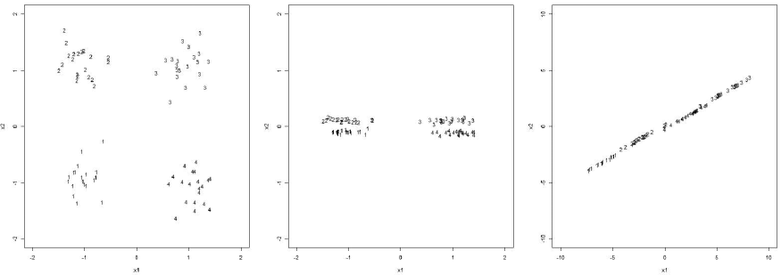
Figure 1: The scatter plots for $X_{I}$, $X_{II}$, and $X_{III}$ of the unit square synthetic data from the left to the right. The most left panel is the original features which have four clusters at the vertices of the unit square with equal size $20$; the middle panel is the features which are transformed by scaling each dimension differently, clusters 1 and 2 are grouped as well as clusters 3 and 4 are grouped; the right panel shows the transformed features are aligned as a straight line.

After $500$ burn-in iterations, we use the $2000$ Markov chains of $B$ samples based on model III to calculate $D$. The resulting heatmap and tree both correctly reveal the true clusters for most of the points (see Figure 2).

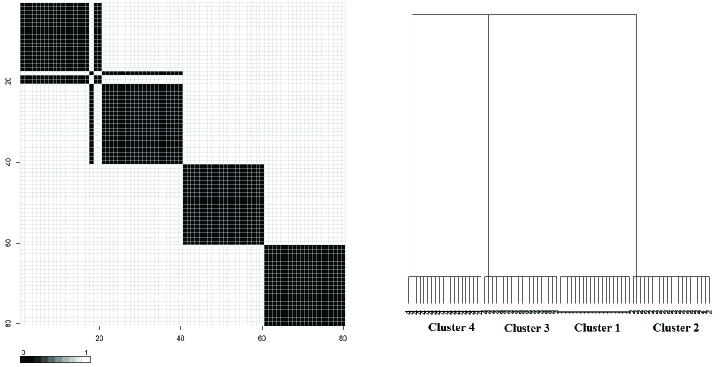
Figure 2: The heatmap of the distance matrix and tree both successfully reveal the true clusters for most of the transformed data $X_{III}$.

Two half-moons data

Further, we apply our approach with model II to the famous two half-moons data (see Figure 3, the left panel) which is generated by the R package of ‘clusterSim’ (Walesiak and Dudek, 2012) with the formula as follows

$$(-0.4+|r\times\cos(\alpha)|,r\times\sin(\alpha))$$ for the first half-moon shape

$$(-|r\times\cos(\alpha)|,r\times\sin(\alpha)-1) \mbox{for the second half-moon shape},$$

where $r\sim\mbox{Uniform}(0.8,1.2),$ and $\alpha\sim\mbox{Uniform}(0,2\pi).$ Both two clusters are not convex. Consequently, it makes distance-based clustering methods such as $K$-means and distance-based hierarchical clustering (Everitt, 1998; Jain et al., 1988) even more difficult to identify the correct clusters. We use the average between-cluster distance and the minimum within-cluster with $1000$ iterations after $610$ burn-in iterations. The resulting heatmap and model tree both show the two half moons clearly.

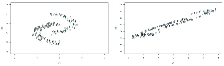
Figure 3: The scatter plots of the original and transformed two half-moons data. Both of the original and the transformed data are difficult for clustering since the clusters are not convex.

In contrast, due to non-convex clusters, the classical $K$-means centering with $K=2$ cannot correctly identify the two half-moons clusters by assigning two convex clusters with centers $(0.1521,0.0922)$ and $(-0.5762,-1.2349)$, respectively. The error rate of the $K$-means approach with $K=2$ is $0.23$ while the average error rate of our approach with model II is $0.115$.

We further transformed the two half-moons data by

$$Y^{\prime}=YA,\;\mbox{where }A=\left(\begin{array}[]{cc}4.1&1.1\\ 2.1&1.1\\ \end{array}\right),$$

and apply our approach based on model III with the maximum within-cluster distance and the minimum between-cluster distance. After the transformation, the two half-moons clusters become thin and long, and are still not well separated. However, our approach with model III can still recover the clusters successfully according to the resulting heatmap and tree (Figure 4) with $1000$ iterations after $400$ burn-in iterations. The error rate of the $K$-means approach with $K=2$ is $0.15$ while the average error rate of our approach with model III is $0.11$.

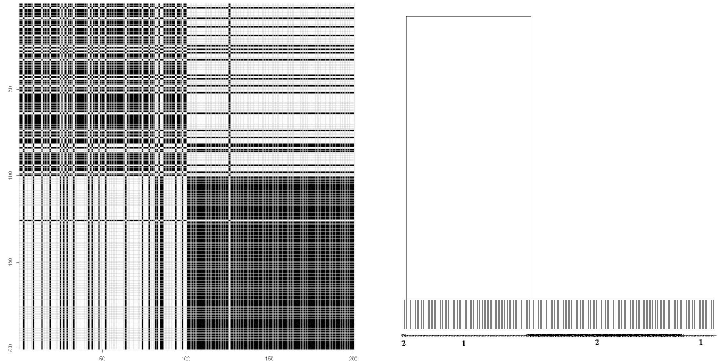
Figure 4: The heatmap of the distance matrix and single-linkage tree both successfully reveal the true clusters for most of the transformed two half-moons data.

5.2 Real data

Model I: Gene expression data of Leukemia patients

Besides the synthetic data, we also evaluate the performance of the proposed approach by using real data. The gene expression microarray data (Lichman, 2013) has been used to study genetic disorder such as identifying diagnostic or prognostic biomarkers or clustering and classifying diseases (Dudoit et al., 2002). For example, Golub et al. (1999) classified patients of acute leukemia into two sub types, Acute Lymphoblastic Leukemia (ALL) and Acute Myeloid Leukemia (AML). For illustration purpose, we use the training set of the leukemia data which consists of 3051 genes and 38 tumor mRNA samples. Pretending we do not know the label information, we would like to cluster the $38$ samples according to their $3051$ features (gene expression levels). The two clusters comprise $27$ ALL cases and 11 AML cases. Since the number of features is larger than the sample size, our approach is not applicable to this dataset directly. Therefore, we first reduce the dimension by projecting the data on the subspace which consists of the first twenty principal components (PC) (Jolliffe, 1986). Note that these PCs are orthonormal which satisfies the assumption of model I. We show the scatter plot of the leukemia data after projecting the original data onto the subspace spanned by the first two principal components $(PC_{1},PC_{2})$ in Figure 5. The resulting tree and heatmap based on model I (Figure 6) both reveal the true clusters with the average within- and between-cluster distances and $1000$ iterations after $500$ burn-in iterations.

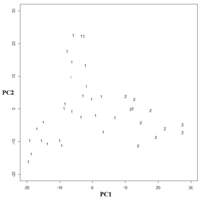
Figure 5: The scatter plot of the leukemia data after projecting the original data onto the subspace spanned by the first two principal components $(PC_{1},PC_{2})$.

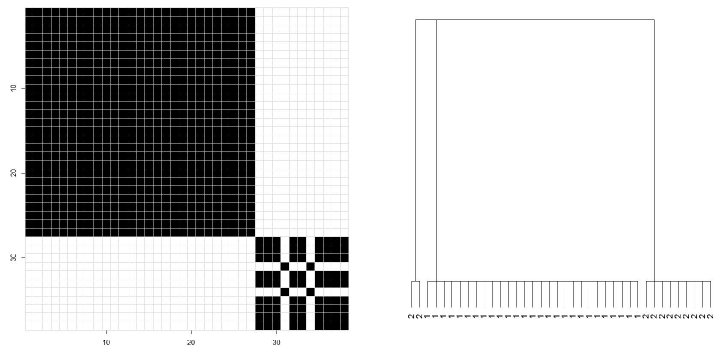
Figure 6: Both the heatmap of the distance matrix and single-linkage tree reveal the two clusters of the leukemia data for most of the points.

Model II: Wine data

We also explore the benchmark wine data (Lichman, 2013). These data are the results of a chemical analysis of wines grown in the same region in Italy but derived from three different cultivars clusters. The cluster sizes are 59, 71, and 48, respectively. The clustering analysis is based on the 13 attributes of the three types of wines with 178 observations. Based on model I, we run $1500$ iterations after $1350$ burn-in iterations with the average between-cluster distance, the minimum within-cluster distance, and $(p_{s},p_{m},p_{k})=(0.09,0.90,0.01)$. The heatmap and tree (Figure 7) both show that the proposed approach with model I can identify the tree clusters for most of the points.

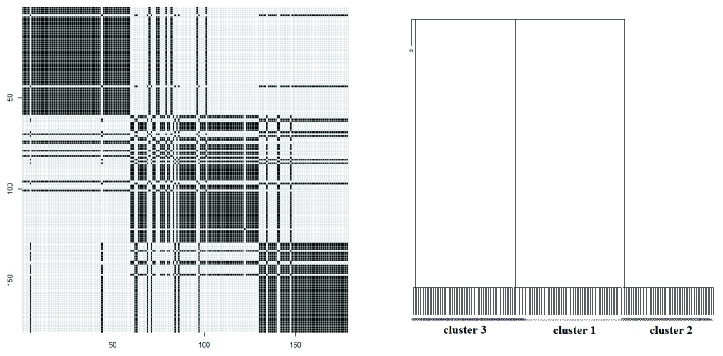
Figure 7: Both the heatmap of the distance matrix and single-linkage tree reveal the three clusters of the wine data for most of the points.

Model III: Geographic coordinate system data of Denmark’s 3D Road Network

This three dimensional road network dataset of geographic coordinates includes the altitude, latitude, and longitude degrees of each road segments in North Jutland in northern Denmark, which is publicly available at the UC Irvine Machine Learning Repository (Kaul, 2013; Lichman, 2013). We obtain 87 observations of 10 different objects which belong to two clusters (cluster 1: objects 1 to 8; cluster 2: objects 9 to 10) based on their longitude and latitude degrees. Note that each objects may have several observations measured from different angles, and the altitude values are extracted from NASA’s Shuttle Radar Topography Mission (SRTM) data (Jarvis et al., 2008). The number of observations of the objects varies from four to twenty. The average geographic coordinates of cluster 1 are $(14.9137,56.9522,8.7564)$, which are the altitude, latitude, and longitude degrees, respectively, and the average geographic coordinates of cluster 2 are $(70.2441,56.6335,9.9938).$ The standard deviations of the altitude, latitude, and longitude degrees of cluster 1 are $(5.2903,0.1330,0.3750)$, and the standard deviations of cluster 2 are $(9.6316,0.0013,0.0054).$ The longitude and latitude degrees determine the true clusters, and they both have much smaller variances than the altitude (see the boxplots in Figure 8). The resulting heatmap and tree (Figure 9) both show the true two clusters with the average within- and between-cluster distances and $1000$ iterations after $500$ burn-in iterations.

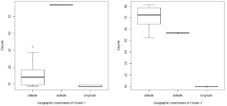
Figure 8: The boxplots show that the altitude has high higher variances for both clusters 1 and 2. The boxplots also indicate that both clusters have higher variances of altitude than latitude and longitude, and the two clusters have very different altitude and latitude degrees on average.

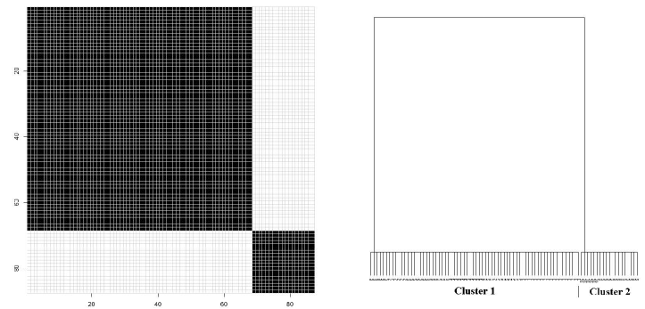
Figure 9: Both the heapmat of the distance matrix and single-linkage tree reveal the two true clusters of the Denmark 3-D road map data.

6 Discussion

We have presented a Bayesian clustering approach which is invariant to different groups of affine transformations. These problems are dealt with an exchangeable partition prior which avoids label-switching problems and the profile likelihoods under three types of covariance structures. Note that the proposed approach does not target the partition maximizing the posterior distribution. Instead, it estimates the expected partition or the distance matrix, which is more reliable for a moderate sample size. It works reasonably well across various applications. Additionally, the transition probability ratio is influenced by the choice of between- and within-cluster distances and the split and merge probabilities $(p_{s},p_{m})$. For example, we choose the minimum within-cluster distance and $(p_{s},p_{m},p_{k})=(0.019,0.98,0.001)$ for both the original and transformed two half-moons data. However, we apply the average between-cluster distance for the original data, but the maximum between-cluster distance for the transformed data. Moreover, when applying other types of the proposed within-cluster distances, the proposed split-merge algorithm does generate the desired clusters after $2000$ burn-in iterations in our experiments. The minimum between-cluster distance tends to connect two nearest clusters and produce a long cluster where neighboring elements in the same cluster have small distances. remain a cluster with a small with-cluster distance (Gower and Ross, 1969; Sibson, 1987). Therefore, we obtain a posterior mean partition matrix instead of a maximum likelihood estimate of partition.

The main contributions of our work include: 1) The proposed three clustering models with three types of covariance structures can handle general cases of affine transformations. In contrast, Vogt et al. (2010) only dealt with the case of model I. 2) The split-merge algorithm can generate partition candidates for the Gibbs sampling much more efficiently (not shown here) than the classical Algorithm 1. It also ensures that the resulting partition-valued Markov chain is ergodic and convergent in distribution. 3) The experiments show the advantages of our cluster process which successfully identifies the true clusters using the proposed distance matrix. In particular if the clusters are not well separated, the distance matrix with probabilistic nature can still reveal the relationships through hierarchical approaches.

The proposed method could be used to extract interesting information from aerial photography, genomic data, and data with attributes under different scales, especially when the nearest neighbors may belong to different clusters in the feature space. R code for implementing the proposed clustering method can be obtained upon request.

References

- Banfield and Raftery (1993) Banfield, J.D. and Raftery, A.E. (1993). Model-based Gaussian and non Gaussian Clustering. Biometrics, 49, 803821.
- Bell (1934) Bell, E.T. (1934). Exponential polynomials. Annals of Mathematics, 35: 258277.
- Ben-Hur and Guyon (2003) Ben-Hur, A. and Guyon, I. (2003). Detecting stable clusters using principal component analysis. In Functional Genomics: Methods and Protocols. M.J. Brownstein and A. Kohodursky (eds.) Humana press, 159182.
- Blei and Jordan (2006) Blei, D. and Jordan, M. (2006). Variational inference for Dirichlet process mixtures. Bayesian Analysis, 1, 121144.
- Chaloner (1987) Chaloner, K. (1987). A Bayesian approach to the estimation of variance components in the unbalanced one-way random-effects model. Technometrics, 29, 323337.
- Crane (2016) Crane, H. (2016). The ubiquitous Ewens sampling formula. Statistical Science, 31, 119.
- Dahl (2005) Dahl, D.B. (2005). Sequentially-allocated merge-split sampler for conjugate and non-conjugate Dirichlet process mixture models. Technical report, Texas A&M University, 2005.
- Dempster (1972) Dempster, A.P. (1972). Covariance Selection. Biometrics, 28(1), 157175.
- Dudoit et al. (2002) Dudoit, S., Fridlyand, J., Speed T.P. (2002). Comparison of discrimination methods for the classification of tumors using gene expression data. Journal of the American Statistical Association, 97(457), 7787.
- Everitt (1998) Everitt, B. (1998). Dictionary of Statistics. Cambridge, UK: Cambridge University Press.
- Ewens (1972) Ewens, W.J. (1972). The sampling theory of selectively neutral alleles. Theoretical Population Biology, 3, 87112.
- Fraley and Raftery (1998) Fraley, C. and Raftery, A.E. (1998). How many clusters? Which clustering methods? Answers via model-based cluster analysis. Computer Journal, 41, 578588.
- Fraley and Raftery (2002) Fraley, C. and Raftery, A.E. (2002). Model-Based Clustering, Discriminant Analysis, and Density Estimation. Journal of the American Statistical Association, 97, 611631.
- Fraley and Raftery (2007) Fraley, C. and Raftery, A.E. (2007). Bayesian Regularization for Normal Mixture Estimation and Model-Based Clustering. Journal of Classification, 24, 155181.
- Geman and Geman (1984) Geman, S. and Geman, D. (1984). Stochastic Relaxation, Gibbs Distributions, and the Bayesian Restoration of Images. IEEE Transactions on Pattern Analysis and Machine Intelligence, 6(6), 721741.
- Golub et al. (1999) Golub, T.R., Slonim, D.K., Tamayo P., Huard C., Gaasenbeek, M., Mesirov, J.P., Coller H., Loh M.L. Downing, J.R., Caligiuri, M.A., Bloomfield, C.D., Lander, E.S. (1999). Molecular Classification of Cancer: Class Discovery and Class Prediction by Gene Expression Monitoring. Science, 531537.
- Gower and Ross (1969) Gower, J.C.; Ross, G.J.S. (1969). Minimum spanning trees and single linkage cluster analysis. Journal of the Royal Statistical Society, Series C, 18(1), 5464.
- Hastings (1970) Hastings, W.K. (1970). Monte Carlo Sampling Methods Using Markov Chains and Their Applications. Biometrika, 57(1), 97109.
- Issacson and Madsen (1976) Isaacson, D.L. and Madsen R.W. (1976). Markov Chains, Wiley, New York, 1976.
- Jain and Dubes (1988) Jain, A.K. and Dubes, R.C. (1988). Algorithms for clustering data. Prentice Hall.
- Jain et al. (1988) Jain, A.K., Murty, M.N. and Flynn, P.J. (1999). Data clustering: a review. ACM Computing Surveys, 31(3), 264323.
- Jarvis et al. (2008) Jarvis, A., H.I. Reuter, A. Nelson, E. Guevara, (2008). Hole-filled SRTM for the globe Version 4, available from the CGIAR-CSI SRTM 90m Database.
- Jolliffe (1986) Jolliffe, I. T. (1986). Principal Component Analysis. Springer-Verlag.
- Kaul et al. (2013) Kaul, M., Yang, B., Jensen, C.S. (2013). Building Accurate 3D Spatial Networks to Enable Next Generation Intelligent Transportation Systems. Proceedings of International Conference on Mobile Data Management (IEEE MDM).
- Kaul (2013) Kaul, M. (2013). Building Accurate 3D Spatial Networks to Enable Next Generation Intelligent Transportation Systems. Proceedings of International Conference on Mobile Data Management (IEEE MDM), June 36 2013, Milan, Italy.
- Lichman (2013) Lichman, M. (2013). (UCI) Machine Learning Repository. University of California, Irvine, School of Information and Computer Sciences.
- MacEachern (1994) MacEachern, S.N. (1994). Estimating normal means with a conjugatestyle Dirichlet process prior. Communication in Statistics: Simulation and Computation, 23, 727741.
- MacQueen (1967) MacQueen, J.B. (1967). Some Methods for classification and Analysis of Multivariate Observations. Proceedings of 5th Berkeley Symposium on Mathematical Statistics and Probability. University of California Press. 281297.
- McCullagh (2008) McCullagh, P. (2008). Marginal likelihood for parallel series. Bernoulli, 14(3), 593603.
- McCullagh and Yang (2006) McCullagh, P. and Yang, J. (2006). Stochastic classification models. Proceedings of the International Congress of Mathematicians (Madrid, 2006), III:669686.
- McCullagh and Yang (2008) McCullagh, P. and Yang, J. (2008). How many clusters? Bayesian Analysis, 3, 101120.
- Neal (2000) Neal, R.M. (2000). Markov chain sampling methods for Dirichlet process mixture models. Journal of Computational and Graphical Statistics, 9, 249265.
- Ng et al. (2001) Ng, A., Jordan, M., and Weiss, Y. (2001). On spectral clustering: Analysis and an algorithm. Advances in Neural Information Processing Systems, 14.
- Ozawa (1985) Ozawa, K. (1985). A stratificational overlapping cluster scheme. Pattern Recognition, 18, 279286.
- Pitman (2006) Pitman, J. (2006). Combinatorial stochastic processes. In Picard, J.(ed.), Ecole d’Ete de Probabilites de Saint-Flour XXXII-2002. Springer, 2006.
- Sibson (1987) Sibson, R. (1973). SLINK: an optimally efficient algorithm for the single-link cluster method. The Computer Journal. British Computer Society, 16(1), 3034.
- Stein (1975) Stein, C. (1975). Estimation of a covariance matrix. Reitz Lecture, IMS-ASA Annual Meeting in 1975.
- Vogt et al. (2010) Vogt, J.E., Prabhakaran, S., Fuchs, T.J., and Roth, V. (2010). The translation-invariant Wishart-Dirichlet process for clustering distance data. Proceedings of the 27 th International Conference on Machine Learning.
- Walesiak and Dudek (2012) Walesiak, M., Dudek, A. (2012). Package clusterSim. http://http://cran.r-project.org/web/packages/clusterSim/clusterSim.pdf (accessed 4.04.12).
- Ward (1963) Ward, J. H., Jr. (1963). Hierarchical Grouping to Optimize an Objective Function. Journal of the American Statistical Association, 58, 236244.