The sandpile revisited: computer assisted determination
of constitutive relations and the breaking of scaling

Abstract

We revisit the problem of the stress distribution in a frictional sandpile under gravity, equipped with a new numerical model of granular assemblies with both normal and tangential (frictional) inter-granular forces. Numerical simulations allow a determination of the spatial dependence of all the components of the stress field as a function of systems size, the coefficient of static friction and the frictional interaction with the bottom surface. Our study clearly demonstrates that interaction with the bottom surface plays a crucial role in the formation of a pressure dip under the apex of a granular pile. Basic to the theory of sandpiles are assumptions about the form of scaling solutions and constitutive relations for cohesive-less hard grains for which no typical scale is available. We find that these constitutive relations must be modified; moreover for smaller friction coefficients and smaller piles these scaling assumptions break down in the bulk of the sandpile due to the presence of length scales that must be carefully identified. After identifying the crucial scale we provide a predictive theory to when scaling solutions are expected to break down. At the bottom of the pile the scaling assumption always breaks, due to the different interactions with the bottom surface. The consequences for measurable quantities like the pressure distribution and shear stress at the bottom of the pile are discussed. For example one can have a transition from no dip in the base-pressure to a dip at the center of the pile as a function of the system size.

I Introduction

Piles of granular matter are all around us, from apples in the market stalls to dunes near the beach. The ubiquity of such aggregates that are typified by sandpiles have raised the interest of scientists for a long time, driven theoretically to understand the shape of such piles (angle of repose) and the distribution of normal and shear stresses. Needless to say these issues are also technologically of high interest from the engineering of silos to the wind-induced migration of sand dunes. Indeed, experimental knowledge has accumulated for over a century 20HF ; 38Hou ; 56Tro ; 81SN ; 99VHCB ; 13AOCRZ . Among the many findings relating to the angle of repose and the stability of such piles, experiments indicated the non-intuitive result that the pressure at the bottom of the pile does not necessarily maximize at the center. Rather, there may appear a dip in the pressure at the center with a ring of maxima (for piles in 3 dimensions) some radius away from the center point. In 2-dimensional piles there may be two maxima in the pressure some distance away from the dip in the center. The existence of such a dip may depend on material parameters and growth protocols like the piling history14ZY , the shape of the grains 93PB , and as we show below, also on the size of the pile and coefficient of static friction $\mu$. Computational investigations corroborated these experimental results 92LCH ; 94BP . The explanation of the dip in the pressure is still not fully settled; in a recent publication 14ZY it was even questioned whether classical continuum theories can predict such dips at all. Below we will show that computer assisted continuum theories can indeed result in a dip in the pressure under the apex of the pile.

Modern theoretical developments began with Edwards’ and Oakeshott’s proposition of the concept of arching 89EO . This concept underlined the relevance of the directional properties of the field of principal axes of the stress tensor. As pointed out in later contributions 95BCC ; 96WCCB ; 97WCC this concept requires an understanding of the spatial solution of the stress tensor, a problem whose mechanics is under-determined. Accordingly, a constitutive relation has to be selected. Since this relation is not dictated by equilibrium mechanics, this selection may be dangerous as it may depend on details of the friction mechanism, the shape of the particles, the protocol of growing the sandpile 99VHCBC etc.

The advent of supercomputers allows us to revisit these interesting issues equipped with a granular model where the effects of friction coefficient, the protocol of growth and the system size can be studied carefully, and where the stress field can be measured accurately. As shown below we find that generically the constitutive relations are hard to guess a-priori, and moreover, they may change with the growth of the pile. For example we will show that a dip in the pressure at the bottom surface under the apex of the pile may develop with the growth of the pile 01BCLO .

A major theoretical assumption made in analyzing the equations of static equilibrium 95BCC ; 96WCCB ; 97WCC is the existence of scaling solutions which for a two-dimensional sandpile in $(x,z)$ coordinates depend only on a scaling variable $S\equiv x\tan\phi/z$ where $\phi$ is the angle of repose. The coordinates $x$ and $z$ are measured from the apex of the pile with $z$ in the direction of gravitational force. The scaling solutions are only tenable when there is no typical length scale in the sandpile other than the system size. We show below that this assumption is broken for small friction coefficients and for small number of grains. One of our tasks is to identify the most relevant length-scale and correlate it with the breaking of scaling and its inevitable consequences. More importantly, even when there exist scaling solutions they are not necessarily of the type assumed in the literature as is shown below. Interestingly, often scaling is only weakly broken in the bulk of the pile, but strongly broken at the bottom where interactions with the supporting surface may differ from the bulk interactions. We will show that the appearance of a pressure dip in the center may very well be related to this strong breaking of scaling.

The structure of the paper is as follows: In Sect. II we describe our numerical model and the results of numerical simulations including the dependence of the angle of repose on the static friction coefficients and the profiles of pressure and shear stresses everywhere in the pile. In Sect. III we briefly review the theoretical background available in the literature. In Sect IV we explain the theoretical modification necessary to get a closer agreement with the simulation results and to provide accurate estimates of the stress and pressure profiles that are of interest. Sect. V examines the observed breakdown in scaling and the necessity for incorporating new length-scales to account for the observed phenomena. Sect. VI offers a summary, conclusions, and some remarks on the road ahead.

II The Model and Simulation Results

II.1 The model

Many models of frictional amorphous materials use time dependent dynamics. In our work we opt to derive a model that can provide complete mechanical equilibration such that at rest the force and the torque on each grain vanishes. To implement an amorphous (non-crystalline) two-dimensional sandpile we construct a model consisting of a 50:50 binary system of disks of two sizes, one with a smaller radius $\sigma_{s}=\lambda$ and the other with a larger radius $\sigma_{\ell}=1.4\lambda$. At every contact between any two disks $i$ and $j$ we assign a normal and a tangential linear spring aligned in parallel and perpendicularly to the radius vector connecting their center of masses. The normal and tangential spring constants are $K_{N}$ and $K_{T}$, respectively. The position of the center of mass of the $i$th disk is denoted as ${\bm{R}}_{i}$ while the vector distance between the center of mass of two particles in contact is denoted as ${\bm{r}}^{ij}$. The unit vector in the direction of ${\bm{r}}^{ij}$ is $\hat{{\bm{r}}}^{ij}$.

The force law for the normal spring, ${\bm{f}}^{ij}_{N}=K_{N}{\bm{n}}^{ij}$, responds to the amount of overlap between particles $i$ and $j$, ${\bm{n}}^{ij}=(\sigma_{i}+\sigma_{j})\hat{{\bm{r}}}^{ij}-{\bm{r}}^{ij}$, as determined by the system configuration. The tangential spring has an analogous force law, ${\bm{f}}_{T}^{ij}=K_{T}{\bm{t}}^{ij}$, however the value of $t^{ij}$ is not readily available from the system configuration. The tangential spring elongation $t^{ij}$ is dependent on the system’s history and needs thus to be tracked along the system’s path. Consider particles $i$ and $j$; when this pair of particles is coming into contact the tangential spring is created and by definition is at its rest length, $t^{ij}=0$. When grazing, the spring is loaded with respect to the degree of grazing, $\Delta t^{ij}=\sigma_{i}\Delta\Phi^{ij}+\sigma_{j}\Delta\Phi^{ji}$. Here $\Delta\Phi^{ij}$ denotes change in angle of the contact point of disc $i$ on disc $j$. For computing the degree of relative rotation we consider the radius to be invariant as long as the compression is small. The expression $\sigma_{i}\Delta\Phi^{ij}$ therefore captures the arc-length and direction along which the point of contact with disc $j$ has moved about particle $i$. During the simulation the actual value of $t^{ij}$ is obtained by summing up the incremental values $\Delta t^{ij}$ until the Coulomb limit is reached. In order to fully define the behavior of particle interaction at the contact it is necessary to differentiate between two types of tangential motions which are rolling and grazing. Two particles rolling on top of each other do not load the spring, $t^{ij}$ remains unchanged. Both types of interaction are taken into account in the present model. Finally, particles $i$ and $j$ share the same springs and it therefore follows, by Newton’s third law, that ${\bm{t}}^{ij}=-{\bm{t}}^{ji}$ and ${\bm{n}}^{ij}=-{\bm{n}}^{ji}$.

The frictional slips are dominated by Coulomb’s law; the maximal deviation of the tangential spring from its rest length is defined by $f_{T,{\rm max}}^{ij}=\mu f_{N}^{ij}$, where $\mu$ is the friction coefficient. When $f_{T}^{ij}=f_{T,{\rm max}}^{ij}$, then the contact breaks and a slip event occurs, redefining the anchoring point of the tangential spring on both particles $i$ and $j$. Following experimental evidence Fineberg we model the slip event by giving up a fixed portion, chosen below as 20%, of the tangential loading. In other words, upon reaching the Coulomb limit we set $t_{\rm new}^{ij}=0.8t_{\rm old}^{ij}$ (representing the movement of the tangential spring’s anchor on the surface of both particles $i$ and $j$).

To construct a sandpile we start with a horizontal “floor” at $h=0$ along the $x$-direction, with one small disk positioned at $x=0$. We then add alternating small and large disks always at $x=0$ with some noise $\delta x$ chosen with a uniform distribution in the range $[-0.1,0.1]$. The particle is positioned at a small clearance in its height that guarantees zero overlap with the highest disk in the pile. After each addition of a disk, we perform conjugate gradient minimization to reach mechanical equilibrium where the forces and torques on each particle sum up to zero. The interaction of the particles with the floor is at our disposal, and we chose to have the same normal law but with with a higher value of $K_{T}$. There is no reason to assume that the grains interact with the floor as they do among themselves. Most of the simulations described below are done with a value of $K_{T}$ for the floor interaction that is double the value in the bulk. We do however test different ratios of the tangential force constants, and see below for details. Finally, the acceleration due to gravity was chosen in the following way: to get a realistic sandpile we should choose the gravitational energy $mg\lambda$ of one particle at height $\lambda$ to be of the order of the elastic energy $\frac{1}{2}K_{N}(\delta\lambda)^{2}$ where $\delta$ is the amount of compression. For $m=1$ for the small particle (and $m=1.96$ for the large particle), $K_{N}=0.1$ and $K_{T}=0.05$ we expect $\delta$ not to exceed, say $10^{-1}$, and thus $g$ should be chosen of the order of $g=0.001$. With this value of $g$ and all the other choices of parameters we get sandpiles that appear physical.

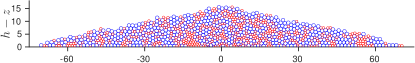
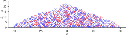
Figure 1: Typical sandpiles grown by the model which employs circular “grains” of two sizes. The friction coefficients are $\mu=0.01$ (upper panel), $\mu=0.1$ (middle panel) and $\mu=1$ (lower panel).

II.2 Results of simulations

Typical results for sandpiles are shown in Fig. 1 for a number of values of the friction coefficient $\mu$. Each of these realizations can be used to define an angle of repose $\tilde{\phi}$ by best fitting to a triangular shape, but of course this angle of repose is a random variable with fluctuations that depend on $N$. We determine the average angle of repose $\phi$ by averaging $\tilde{\phi}$ over ${{\mathcal{N}}}$ realizations. For example we created sandpiles with ${\mathcal{N}}=718,1123,555$ for $\mu=0.01,0.1,1$, respectively. The relation between the angle of repose $\phi$ at a given size $N$ and $\mu$ for given material parameters $K_{N},K_{T}$ and for the fixed circular disks in this model is shown in Fig. 2. One sees that $\tan\phi$ starts as a linear function of $\mu$ for small $\mu$, $\tan\phi\approx C_{1}\mu$ where $C_{1}\approx 2.5$. At larger values of $\mu$, $\tan\phi$ saturates with a maximal angle of repose $\phi_{\rm max}\approx 24^{\circ}$. The function shown in Fig. 2 can be fitted using a Padé approximation as

$$\tan\phi\approx\frac{C_{1}\mu}{1+C_{2}\mu}\ ,\quad\frac{C_{1}}{C_{2}}=\tan\phi_{\rm max}\ .$$ (1)

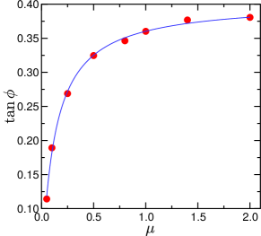
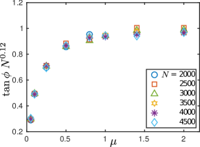
Figure 2: Upper panel: $\tan\phi$ as a function of the friction coefficient $\mu$ for a given system size $N=3000$. The fitting function in continuous blue line is $\tan\phi\approx C_{1}\mu/(1+C_{2}\mu)$, cf. Eq. 1. Lower panel: data collapse of $\tan\phi$ for different values of system size $N$ as a function of $\mu$. It is possible that for much larger values of $N$ the angle or repose reaches an asymptotic value.

It should be noted that for systems sizes simulated here the angle of repose is a weak function of the system size $N$, decreasing approximately like $N^{-0.12}$ for all the values of $\mu$. In other words, for different system sizes $N$ and different values of $\mu$ one can find a master curve for which the angle of repose shows data collapse by plotting $\tan\theta\times N^{0.12}$ vs. $\mu$, see Fig. 2 lower panel. A similar weak dependence of the angle of repose on system size for small size sandpiles had been found numerically before, cf. Ref. 94BP .

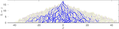
Figure 3: Typical appearance of the force chains in a sandpile of size $N=600$ and $\mu=0.35$.

An interesting and often studied characteristic of granular compressed media is the geometry of force chains. To present these one needs to choose a threshold for the inter-particle forces ${\bm{f}}_{ij}$ at the contacts and plot only those forces that exceed the threshold. This is somewhat arbitrary and is in the eyes of the beholder. Choosing the force chains to be system spanning Somfai we get typical results as shown in Fig. 3. This figure underlines the existence of a typical scale that will be discussed below, i.e. the typical distance between bifurcations of the force chains.

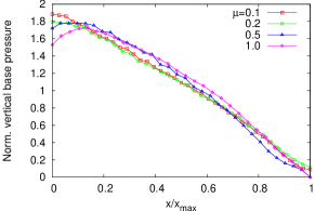
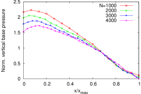
Figure 4: Base pressure distribution normalized by $Mg/(2x_{max})$. Upper panel: systems consisting of $4000$ grains with different $\mu$. Lower panel: $\mu=1$ but with different number of grains, $N$.

Fig. 4 shows the pressure distribution along the bottom (base pressure) of the pile. The base pressure is defined to be the amplitude of the force acting on each grain fixed on the bottom and averaged in symmetric cells of dimension $4.0\lambda$. The base pressure is normalized by $Mg/(2x_{max})$ where $M$ is the total mass of the pile and $x_{max}$ is the maximum horizontal spread from the center of the pile. In the upper panel of Fig. 4 we show that there is a transition from no-dip to dip as $\mu$ is increased. The number of grains $N$ is fixed at $4000$ for all the curves. In the lower panel of Fig. 4 we show that even for a fixed $\mu$ ($=1$ in the plot) the dip-height reduces very sharply with decreasing $N$. For $\mu=1$ we see pressure dip even for very small piles $N=500$. However, for lower $\mu$ we observe a no-dip to dip transition as $N$ is increased. In Fig. 5 we plot the critical number of grains $N_{c}$ below which no pressure dip is observed at the corresponding $\mu$.

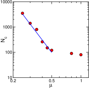
Figure 5: Number of grains below which no pressure dip has been observed, as a function of $\mu$.

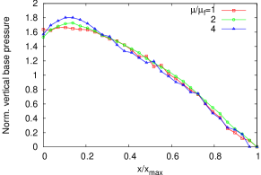
Figure 6: Base pressure distribution normalized by $Mg/(2x_{max})$ for three different particle-floor friction coefficient ${\it viz}$ $\mu_{f}=1.0,2.0,4.0$. The particle-particle friction coefficient $\mu=1$.

Another striking observation is that the dip in the base-pressure depends strongly on the floor to particle friction coefficient. The dip height increases with the increase in the floor-particle friction coefficient which we denote by $\mu_{f}$. This is shown in Fig. 6 where we plot the distribution of normalized base pressure for three different floor-particle friction coefficient ${\it viz}$ $\mu_{f}=1.0,2.0,4.0$, particle-particle friction coefficient $\mu=1$ and the number of grains being $N=4000$ for all the cases. In all the simulations in which we do not report a different value we have used $\mu_{f}=2\mu$.

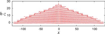
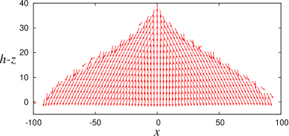
Figure 7: Direction of the principal axis $\Psi(x,z)$ of the stress in the sandpile for two different values of the friction coefficient. Upper panel: $\mu=0.1$ Lower panel $\mu=1$. A similar figure for $\mu=0.01$ is not shown since it does not display well.

A quantity of crucial theoretical interest which is used below in the context of constitutive relations is the direction of the principal axis of the stress tensor in the pile. We define $\Psi(x,z)$ as the angle between the principal axis and the $z$-axis. To obtain our numerical calculation of $\Psi$ we consider the aforementioned ${\mathcal{N}}$ copies of sandpiles with a given value of $\mu$, and system size $N$. For each realization we compute the stress field on plaquettes of sizes $2.4\lambda\times 2.4\lambda$ using the standard algorithms 07IMPS . We average the obtained stress field in each plaquette over all the realizations. Finally, we determine the principal axis $\Psi(x,z)$ using Eqs. (4) below. Typical results for $\mu=0.1$ and 1 are shown in Fig 7. The image for $\mu=0.01$ does not display well. The reader should note the very strong fluctuations, even after averaging on many independent samples of $\Psi(x,z)$ on the surface of the sand piles. We will argue below that these fluctuation are responsible in part for destroying the scaling assumptions.

III Theoretical background

An extremely useful and important review is provided by Ref. 97WCC . For the two-dimensional sandpile (which corresponds to our simulations) the fundamental equations for the stress field at equilibrium read

$$\partial_{x}\sigma_{xx}+\partial_{z}\sigma_{xz} = 0$$

$$\partial_{x}\sigma_{xz}+\partial_{z}\sigma_{zz} = mg/\lambda^{2}\ ,$$ (2)

where $mg$ is the gravity force on a grain of mass $m$ and area $\lambda^{2}$. The coordinate $z$ is measured from the apex of the pile and $x$ is measured from the symmetry axis. Note that these equations are under-determined since there are two equations for the three independent components of the stress tensor $\sigma_{xx},\sigma_{xz}=\sigma_{zx}$ and $\sigma_{zz}$. Using the trace and determinant of the stress tensor as invariants one can find the angle of inclination $\Psi$ between the principal axis of the stress and the $z$ axis. Defining the invariants

$$P \equiv \frac{1}{2}(\sigma_{xx}+\sigma_{zz})$$

$$R^{2} \equiv \frac{1}{4}(\sigma_{zz}-\sigma_{xx})^{2}+\sigma^{2}_{zx}\ ,$$ (3)

one can then write

$$\sigma_{xx} = P-R\cos(2\Psi)\ ,$$

$$\sigma_{zz} = P+R\cos(2\Psi)\ ,$$

$$\sigma_{xz} = R\sin(2\Psi)\ .$$ (4)

The maps of principal axes shown in Sect. II were computed with the help of these equations.

Discussing the stability of the sand pile, we recall that the simulations employ three independent material parameters, i.e. $K_{N}$, $K_{T}$ and $\mu$. It is customary to introduce a phenomenological material constant, sometime denoted as $\tan\phi^{*}$ which is referred to as the angle of internal friction and used in the limit of stability

$$|\sigma_{nt}|\leq\tan\phi^{*}\sigma_{nn}\ ,$$ (5)

where $\sigma_{nn}$ and $\sigma_{nt}$ are the normal and tangential components of the stress on any chosen plane. We find in our simulations that $\phi^{*}$ is equal to the angle of repose $\phi$. Eq. (5) can be recast, using the invariants $P$ and $R$ into a stability condition of the form

$$Y\equiv\frac{R}{P\sin\phi}\leq 1\ ,$$ (6)

everywhere in the sandpile. Specifically on the surface of the pile we expect marginal stability such that the inequalities (5) and (6) are saturated.

Although Eqs. (2) are under-determined, they do allow seeking scaling solutions in the form

$$\sigma_{xx} = \frac{mgz}{\lambda^{2}}s_{xx}(S)\ ,$$

$$\sigma_{xz} = \sigma_{zx}=\frac{mgz}{\lambda^{2}}s_{xz}(S)\ ,$$

$$\sigma_{zz} = \frac{mgz}{\lambda^{2}}s_{zz}(S)\ ,$$ (7)

where $S\equiv x\tan\phi/z$. Plugging this ansatz into Eqs. (2) results in the scaled equations

$$\tan\!\phi~{}s^{\prime}_{xx}+s_{xz}-Ss^{\prime}_{xz} = 0\ ,$$

$$\tan\!\phi~{}s^{\prime}_{xz}+s_{zz}-Ss^{\prime}_{zz} = 1.$$ (8)

where $s^{\prime}\equiv ds/dS$.

To close these equations one needs a constitutive relation. Using Eq. (4), dividing $\sigma_{xx}$ by $\sigma_{xz}$ and rearranging we can derive the following relation

$$s_{xx}(S)=s_{zz}(S)-2\cot\big{(}2\Psi(S)\big{)}s_{zx}(S)\ .$$ (9)

This equation is of course useless as long as we do not know $\Psi(S)$. In general we are not even guaranteed that $\Psi(S)$ exists as function of one variable. In the general case we should use instead of $\Psi(S)$ a function of two variables $\Psi(S,z)$. The dependence on one variable $S$ means that as the pile grows $S$ is changing and with it so does $\Psi(S)$. The strategy is therefore to determine the function $\Psi(S)$ from the numerics, and then to use Eq. (9) as the constitutive relation that will close the problem and will allow us to determine the stress field everywhere in the pile.

III.1 Numerical Integration of the Scaling Solutions

Eqs. (8) and (9) together with the boundary conditions $s_{xz}(S=1)=0$ and $s_{zz}(S=1)=0$ admit solutions close to the free surface $S=1$ that are linear in $(1-S)$. These linear solutions as $S\to 1$ demand that $\cot(2\Psi(S=1))=\tan\phi$ or, equivalently 95BCC ; 96WCCB ; 97WCC , that

$$\Psi(S=1)=\frac{\pi-2\phi}{4}\ .$$ (10)

There is less information about $\Psi(S=0)$ but simulations suggest (see below) that $\Psi(S=0)=0$. In other words the principal axis ends up pointing in the direction of the gravity field as $S=0$ under the apex of the sandpile.

As a first attempt in solving the problem we will use a fit to the numerical data that satisfies the boundary condition (10). We will see that this solution does not predict a dip in the pressure at $S=0$. Examining our numerical estimate of $\Psi(S)$, see Fig. 8,

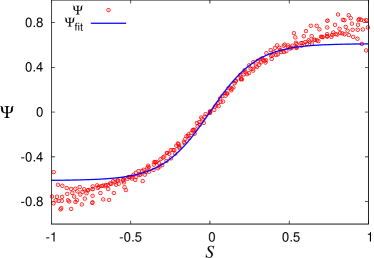
Figure 8: The fitting function $\Psi_{\rm fit}(S)$ compared to the actual data for $\mu=1$.

we choose a global parameterized fit of the form

$$\Psi_{\rm fit}(S)=\frac{(\pi-2\phi)}{4}\frac{\tanh(\beta S)}{\tanh\beta}\ .$$ (11)

We find that with $\beta=3$ (cf. Fig. 8) we get a reasonable fit to the data that obeys Eq. (10). A consequence of the agreement of our parameterized $\Psi_{\rm fit}(S)$ with the theoretical limit $\Psi(S=1)=(\pi-2\phi)/4$ as in Eq. (11) is that the solution becomes marginally stable on the surface of the pile. This is physically pleasing since one expects the outer surface to be just marginally stable and ready to avalanche with every addition of a new particle. If we allowed the function $\Psi_{\rm fit}(S)$ to asymptote to the correct limit found in the simulations, which is higher than the expected theoretical value, it would lead to the loss of marginal stability at the surface. The solutions would become either stable or unstable at the surface of the sandpile.

The ordinary differential equations that should be solved are derived in the next subsection. Here we show that the strategy of integrating them from the outer boundary does not yield acceptable results. Starting from the given boundary condition we can solve numerically the linear coupled inhomogeneous ode’s (13) starting at the surface of the sand pile and integrating inward. In Fig. 9 we present solution for the three independent components of the stress tensor for different values of the angle of repose.

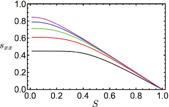
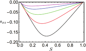
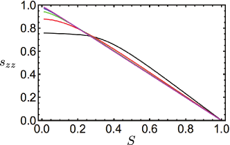
Figure 9: The numerical results for the functions $s_{xx}(S)$, $s_{xz}(S)$ and $s_{zz}(S)$ for sandpiles with different angle of repose found by solving Eqs. 8 inwards from $S=1$ where the boundary conditions are known.

The result is disappointing, there is no tendency to form a dip in any of the stress components at the center of the pile. Should we believe these solutions?

To see that these results are in fact untenable we should examine the stability of these continuum solutions. To this aim we return to Eq. (6) and plot in Fig. 10 the value of $Y^{2}(S)$ for different values of the angle of repose.

Figure 10: The test of stability of the scaling solutions using $Y^{2}(S)$ for the same values of $\phi$ as in Fig. 9.

We immediately note that deep in the sandpile, exactly where the peak to dip transitions can be expected to occur these scaling solutions become unstable, cf. Eq. (6).

We conclude that the scaling solutions become unstable deep in the sandpile (see Fig. 10), especially near the center of the sandpile. It is just here, however, that the very interesting transitions in the pressure at the bottom of the sandpile from showing a peak to showing a dip appear. We thus need to forsake the straightforward scaling solutions and examine the situation with greater scrutiny.

IV Computer assisted theory

IV.1 Numerical evidence for the breaking of scaling

Having extracted the stress tensor in the pile as a function of $(x,z)$ we can compute the theoretically relevant tensors $s_{xx}(S,z)$, $s_{xz}(S,z)$ and $s_{zz}(S,z)$. These are plotted for $\mu=1$ and $\phi\approx 0.36=\pi/8.73$ for different values of $z$, in the three panels of Fig. 11. In comparing the plots in Fig. 9 and Fig. 11 one should observe that the model simulations are not precisely scaling and depend explicitly on $z$. This should not be confused with the theoretical curves in Fig. 9 that pertain to different angles of repose but that show perfect scaling.

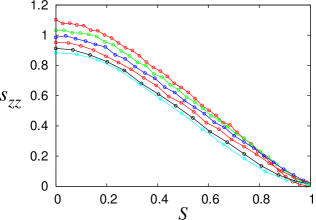
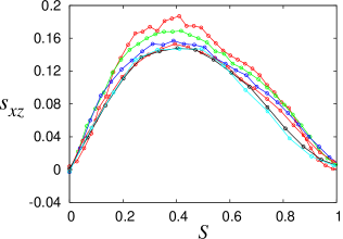
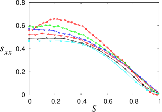
Figure 11: The simulation results for the functions $s_{zz}(S,z)$, $s_{xz}(S,z)$ and $s_{xx}(S,z)$ for one angle of repose, $\phi\approx\pi/8.73$ which pertains to $\mu=1$. The different curves are now due to the fact that the scaling assumption is broken, and the functions are shown at different heights $z$. The reader should not confuse these figures with Fig. 9 where the different color represent different angles of repose. The color code here refers to the following values of $z$ as measured from the apex: red : $z=32.35$, green: $z=27.55$, blue: $z=22.75$, magenta: $z=17.95$, black: $z=13.15$, cyan: $z=8.35$.

Clearly, scaling appears to be broken and the ”scaling” solutions $s_{xx}(S)$, $s_{xz}(S)$ and $s_{zz}(S)$ are actually functions of both $(S,z)$. The same problem exists with the function $\Psi(S)$ as discussed in the next subsection.

IV.2 The Direction Of the Principal Stress Axis

Solving Eqs. (8) is impossible without adding an explicit form for the principal stress axis $\Psi$ into the constitutive relation Eq. (9) to close the mathematical problem. A number of constitutive relations have been proposed; we find the so-called “Fixed Principal Axis” quite plausible, since it is based on the physical assumption that once the principal axis of the stress was determined near the surface, it gets buried unchanged with the growth of the sandpile. Note that this makes no assumption about the magnitude of the principal stresses, only about their directions. Nevertheless our simulations are not in full agreement with this assumption, neither near the surface nor deep in the pile. We therefore turn now to the analysis of the principal axis of the stress field as seen in simulations.

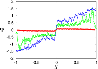
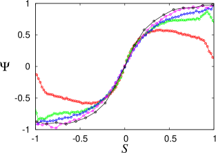
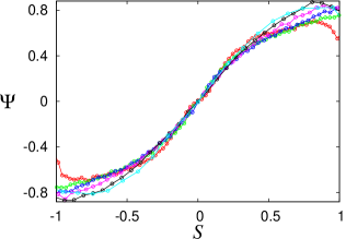
Figure 12: The angle $\Psi(S,z)$ as a function of $S$ computed for sandpiles created with $\mu=0.01$ (upper panel), $\mu=0.1$ (middle panel) and $\mu=1$ (lower panel). The different colors correspond to different heights $z$. If the scaling assumption prevailed all these plots should collapse. Note that for $\mu=1$ the scaling assumption is close to being obeyed but it breaks totally for $\mu=0.01$. The color code refers to different values of $z$ as measured from the apex which are: upper panel; red : $z=8.28$, green: $z=5.88$, blue: $z=3.48$. Middle panel; red : $z=23.42$, green: $z=18.62$, blue: $z=13.82$, magenta: $z=9.02$, black: $z=4.22$. Lower panel; red : $z=32.35$, green: $z=27.55$, blue: $z=22.75$, magenta: $z=17.95$, black: $z=13.15$, cyan: $z=8.35$.

When the scaling assumptions discussed above are valid, $\Psi$ should be a function of $S$ only, $\Psi(S)$. If scaling breaks down this function depends on both $S$ and $z$. The numerical evidence is shown in Fig. 12. The three panels present $\Psi(S,z)$ at different heights $z$ in the sandpile. If the scaling assumption were corroborated by the simulation we would expect that all these curves would collapse on a single function $\Psi(S)$. We learn that for large values of the friction coefficient $\mu$, which correspond to large angle of repose, the scaling assumption is reasonably obeyed. The scaling assumption deteriorates when $\mu$ and the angle of repose decrease, until eventually it breaks down entirely. Notice however that the actual function $\Psi(S)$, even when the scaling assumption is relatively acceptable does not agree with many constitutive relations that were assumed in the literature, which are often piece-wise linear, cf. Refs. 95BCC ; 96WCCB ; 97WCC and reference therein.

For large of values of $\mu$, $\Psi(S,z)$ does indeed approach a scaling function $\Psi(S)$ except for coordinates at the bottom of the pile, cf. the curve shown in red in lower panel of Fig. 12. Note that even in those cases $\lim_{S\to 1}\Psi(S)$ is not very close the theoretical expectation Eq. (10), which for $\mu=1$ and $\phi=0.36$ predicts $\Psi(S=1)\approx 0.61$. We propose that this discrepancy stems from the large fluctuations in the surface geometry which manifests itself in the large fluctuations in $\Psi$ seen in Fig. 7 at the surface, and see below for more details.

IV.3 Analytic solutions Valid Near The Center Of The Sandpile

When we integrate the scaled equations (8) from the surface of the sandpile using the boundary conditions $s_{xz}(S=1)=0$ and $s_{zz}(S=1)=0$ the solutions become unstable deep in the sandpile. We therefore change our approach here and attempt to supplement our numerical integration of Eqs. (8) and Eq. (9) with analytical approaches valid deep in the sandpile. Thus substituting Eq. (9) in Eqs. (8) and rearranging we find for

$${{\bm{s}}}(S)=\left(\begin{array}[]{c}s_{xz}(S)\\ s_{zz}(S)\\ \end{array}\right).$$ (12)

the set of coupled linear inhomogeneous ordinary differential equations

$${\bm{A}}(S){\bm{s}}^{\prime}(S)+{\bm{D}}(S){\bm{s}}(S)=\left(\begin{array}[]{c}0\\ 1\\ \end{array}\right).$$ (13)

Here

$${\bm{A}}(S)\equiv\left(\begin{array}[]{cc}-\Big{(}2\tan\phi\cot\big{(}2\Psi(S)\big{)}+S\Big{)}&\tan\phi\\ \tan\phi&-S\\ \end{array}\right).$$ (14)

and

$${\bm{D}}(S)\equiv\left(\begin{array}[]{cc}1+\frac{4\tan\phi}{\sin^{2}\big{(}2\Psi(S)\big{)}}\Psi^{\prime}(S)&0\\ 0&1\\ \end{array}\right).$$ (15)

We cannot simply integrate from the center of the sandpile ($S=0$) towards the surface, however, as we do not possess the required boundary value for $s_{zz}(0)$. We will therefore take another approach.

Eq. (13) is in principal exactly soluble as it is a linear inhomogenous equation, and we also have a good knowledge of the symmetry properties of all the relevant variables near the center of the sandpile. We can therefore find a solution that is valid order by order in $S$ for small $S$ near the center of the sandpile.

First we will write the general solution of Eqs (13) as the sum of a particular solution and a complementary solution of the associated homogeneous equation as ${\bm{s}}(S)={\bm{s}}_{p}(S)+{\bm{s}}_{hom}(S)$ where the particular solution is

$${\bm{s}}_{p}(S)=\left(\begin{array}[]{c}0\\ 1\\ \end{array}\right).$$ (16)

and the complementary solution obeys (using from now on the notation $t\equiv\tan\phi$)

$$d{\bm{s}}_{hom}(S)/dS+{\bm{B}}(t,S){\bm{s}}_{hom}(S)=\left(\begin{array}[]{c}0\\ 0\\ \end{array}\right).$$ (17)

Here ${\bm{B}}={\bm{A}}^{-1}{\bm{D}}$ or

$${\bm{B}}(t,S)\equiv-{\det{\bm{A}}}^{-1}$$ (18)

$$\left(\begin{array}[]{cc}S\big{(}1+\frac{4t}{\sin^{2}\big{(}2\Psi(S)\big{)}}\Psi^{\prime}(S)\big{)}&t\\ t\big{(}1+\frac{4t}{\sin^{2}\big{(}2\Psi(S)\big{)}}\Psi^{\prime}(S)\big{)}&\Big{(}2t\cot\big{(}2\Psi(S)\big{)}+S\Big{)}\end{array}\right)\ .$$ (21)

where $\det{\bm{A}}(t,S)=S(2t\cot(2\Psi(S)\big{)}+S)-t^{2}$.

Eq. (17) can be integrated exactly from $S=0$ to $S=1$ and using the boundary outer boundary conditions

$${\bm{s}}_{hom}(1)=\left(\begin{array}[]{c}0\\ -1\\ \end{array}\right).$$ (22)

we can find an explicit equation for ${\bm{s}}(S)$ in the form

$${\bm{s}}(t,S)=(I-{\bm{M}}^{-1}(t,S){\bm{M}}(t,1))\left(\begin{array}[]{c}0\\ 1\\ \end{array}\right).$$ (23)

where

$${\bm{M}}(t,S)=\exp{\int_{0}^{S}{\bm{B}}(t,S^{\prime})dS^{\prime}}.$$ (24)

Eq. 24 is a $2\times 2$ matrix that depends explicitly on the scaling variable $S$ and the angle of repose $\phi$ through the variable $t\equiv\tan{\phi}$. It is a global function of $S$. For example, we can find an explicit expression for $s_{zz}(t,0)=1-M(t)$ at the center of the sand pile and consequently an expression for the pressure at the center of the sandpile in terms of a global integral over the whole sandpile

$$M(t)=\big{(}\exp{\int_{0}^{1}{\bm{B}}(t,S^{\prime})dS^{\prime}}\big{)}_{22}.$$ (25)

We are especially interested in the behavior of the scaling variables near the center of the sandpile (small $S$) as this will allow us to see any peak to dip transitions transitions in the stress. We shall now expand the angle of the principal axis near the center of the sandpile as

$$\Psi(S)=\alpha S-\beta S^{3}+\gamma S^{5}+\cdots\ ,$$ (26)

using the fact that this angle is an odd function of $S$ (see Fig. 12). We will assume that $\alpha$ and $\beta$ are dimensionless parameters dependent on the material properties of the sandpile.

We are now in a position to calculate the series expansion of the complete stress tensor as a series expansion in $S$. Using the symmetry properties of the scaled stress tensor components we write

$$s_{xz}(t,\alpha,S) = s_{xz1}(t,\alpha)S+s_{xz3}(t,\alpha)S^{3}+s_{xz5}(t,\alpha)S^{5}+\cdots$$

$$s_{zz}(t,\alpha,S) = s_{zz0}(t,\alpha)+s_{zz2}(t,\alpha)S^{2}+s_{zz4}(t,\alpha)S^{4}+s_{zz6}(t,\alpha)S^{6}+\cdots$$

$$s_{xx}(t,\alpha,S) = s_{xx0}(t,\alpha)+s_{xx2}(t,\alpha)S^{2}+s_{xx4}(t,\alpha)S^{4}+s_{xx6}(t,\alpha)S^{6}+\cdots$$

Substituting expressions  (LABEL:st) into the scaled continuum Eq. (8b), we can expand order by order in $S$ and in this manner get explicit expressions for the following coefficients of the stress tensor:

$$s_{xz1}(t) = \frac{1-s_{zz0}}{t}$$

$$s_{xz3}(t,\alpha) = \frac{s_{zz2}}{3t}$$

$$s_{xz5}(t,\alpha) = \frac{3s_{zz4}}{5t}$$

$$s_{xz7}(t,\alpha) = \frac{5s_{zz6}}{7t}.$$ (28)

Now, substituting expressions  (LABEL:st) into Eq. (8a), we can again expand order by order in $S$ and get the following relations:

$$s_{xx2}(t) = 0$$

$$s_{xx4}(t,\alpha) = \frac{s_{xz3}}{2t}=\frac{s_{zz2}}{6t^{2}}$$

$$s_{xx6}(t,\alpha) = \frac{2s_{xz5}}{3t}=\frac{2s_{zz4}}{5t^{2}}$$

$$s_{xz7}(t,\alpha) = 0,$$ (29)

Finally, we substitute expressions  (LABEL:st) into the constitutive equation Eq. (9) and obtain the following expressions:

$$s_{xx0}(t,\alpha) = s_{zz0}-\frac{s_{xz1}}{\alpha}$$

$$s_{xx2}(t,\alpha) = s_{zz2}-\frac{s_{xz3}}{\alpha}+\frac{4\alpha s_{xz1}}{3}-\frac{\beta s_{xz1}}{\alpha^{2}}$$

$$s_{xx4}(t,\alpha) = s_{zz4}-\frac{s_{xz5}}{\alpha}+\frac{4\alpha s_{xz3}}{3}-\frac{\beta s_{xz3}}{\alpha^{2}}+\frac{16\alpha^{3}s_{xz1}}{45}$$

$$- \frac{4\beta s_{xz1}}{3}-\frac{\beta^{2}s_{xz1}}{\alpha^{3}}+\frac{\gamma s_{xz1}}{\alpha^{2}}$$

$$s_{xx6}(t,\alpha) = s_{zz6}+\frac{128\alpha^{5}s_{xz1}}{945}-\frac{\beta^{3}s_{xz1}}{\alpha^{4}}-\frac{16\alpha^{2}\beta s_{xz1}}{15}$$ (30)

$$+ \frac{4\gamma s_{xz1}}{3}+\frac{2\beta\gamma s_{xz1}}{\alpha^{3}}-\frac{\beta^{2}s_{xz3}}{\alpha^{3}}+\frac{16\alpha^{3}s_{xz3}}{45}$$

$$- \frac{4\beta s_{xz3}}{3}+\frac{\gamma s_{xz3}}{\alpha^{2}}-\frac{\beta s_{xz5}}{\alpha^{2}}+\frac{4\alpha s_{xz5}}{3}.$$

Using $s_{zz0}(t)=1-M(t)$, we can further simplify the above expressions to obtain

$$s_{zz0}(t) = 1-M(t)$$

$$s_{xz1}(t) = M(t)/t$$

$$s_{xx0}(t,\alpha) = 1-M(t)(1+\frac{1}{\alpha t})$$

$$s_{zz2}(t,\alpha) = \frac{M(t)(4\alpha^{3}-3\beta)}{\alpha(1-3t\alpha)})$$

$$s_{xz3}(t,\alpha) = \frac{M(t)(4\alpha^{3}-3\beta)}{3t\alpha(1-3t\alpha)}$$

$$s_{xx2}(t,\alpha) = 0\ ,$$ (31)

$$s_{zz4}(t,\alpha) = \frac{M(t)(-4\alpha^{4}(5+8t\alpha(-2+t\alpha))+15\alpha(1+8t\alpha(-1+t\alpha))\beta+90t^{2}\beta^{2}+30t\gamma(1-3t\alpha))}{6t\alpha(-1+3t\alpha)(-3+5t\alpha)}$$

$$s_{xz5}(t,\alpha) = \frac{M(t)(-4\alpha^{4}(5+8t\alpha(-2+t\alpha))+15\alpha(1+8t\alpha(-1+t\alpha))\beta+90t^{2}\beta^{2}+30t\gamma(1-3t\alpha))}{10t^{2}\alpha(-1+3t\alpha)(-3+5t\alpha)}$$

$$s_{xx4}(t,\alpha) = \frac{M(t)(4\alpha^{3}-3\beta)}{6t^{2}\alpha(1-3t\alpha)}$$

$$s_{zz6}(t,\alpha) = 0$$

$$s_{xx6}(t,\alpha) = \frac{M(t)(-4\alpha^{4}(5+8t\alpha(-2+t\alpha))+15\alpha(1+8t\alpha(-1+t\alpha))\beta+90t^{2}\beta^{2}+30t\gamma(1-3t\alpha))}{15t^{3}\alpha(-1+3t\alpha)(-3+5t\alpha)}$$ (32)

Let us analyze $s_{zz2}(t,\alpha)=[M(t)/\alpha)(4\alpha^{3}-3\beta)/(1-3t\alpha)]$ more closely. We first note that if $(4\alpha^{3}-3\beta)=0$ the coefficient goes through zero. Thus a critical value of the principal axis gradient exists, given by

$$\alpha_{c}=(3\beta/4)^{1/3}.$$ (33)

This will create the well known peak to dip transition in sand pile pressure at the center of the sandpile. There is also a second transition apparent in the coefficients. We can also see that at lower values of $\alpha$ a singularity develops in the coefficients when $(1-3t\alpha)=0$. Or

$$\alpha_{sing}=\frac{1}{3t}.$$ (34)

A fitting of principal stress direction $\Psi(S)$ near the center of the pile using Eq. (26) is shown in Fig. 13. Now, using these fitted values of $\beta$ and $\gamma$, we compute $s_{zz}(\alpha,S)$ and $s_{xx}(\alpha,S)$ for $t=\pi/9.0$, which corresponds to the angle of repose for $\mu=1$. These functions are shown in Fig. 14. We see that there is a transition in $s_{zz}(\alpha,S)$ from a peak ($s_{zz2}<0$) to a dip ($s_{zz2}>0$) as $\alpha$ decreases. This is in accordance with our simulation results as smaller values of $\alpha$ will correspond to a higher $\mu$. A similar but less prominent dip is also observed in $s_{xx}(\alpha,S)$ in the same range of $\alpha$. Furthermore, we also find a singularity in the second and higher order coefficients at $\alpha=1/(3t)\approx 0.955$, but it is not clear at present whether this is an observable singularity. The reason being that Eq. (33) depends on the parameter $\beta$ and for real materials this may lead to $\alpha_{crit}\gg\alpha_{sing}$ for sandpiles.

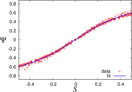
Figure 13: A plot of principal stress direction $\Psi(S)$ near the center of the pile. Red circles are the raw data obtained from the simulation and the blue curve is a fit (Eq. (26)) to the data. The fitting parameters are $\alpha=1.64052,\beta=2.77268,\gamma=3.872$.

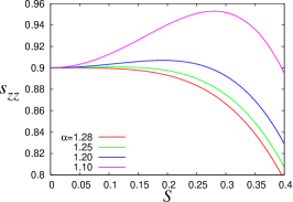
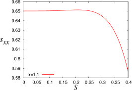
Figure 14: Plots of $s_{zz}$ (upper panel) and $s_{xx}$ (lower panel) as a function of $S$ and $\alpha$ near the center of the sandpile. Note the transition from a peak to a dip as the principal axis gradient $\alpha$ decreases. We have chosen $\phi=\pi/9.0,\beta=2.77268$ and $\gamma=3.872$ for these plots.

We can conclude that the theory proposed here is in agreement with the observed phenomenology concerning the creation of a dip in the base pressure. What remains is to consider some of the physical reasons why a breakdown in scaling may exist in sandpiles, and how this phenomenon is related to the value of $\mu$, or equivalently to the value of the angle of repose.

V New Length Scales

It appears that there exists a clear transition at some critical angle of repose, say $\phi_{\rm crit}$, below which scaling solutions stop being stable inside the sandpile. This does not mean that there cannot exist stable solutions to the mechanical equilibrium problem, but rather, as we see in the simulations, scaling is broken and the solutions become heterogeneous, dependent on both $x$ and $z$. Thus in some sense the theory predicts its own demise as is corroborated by the simulations. This is not a trivial remark. We have taken a “reasonable” constitutive relation fitted to the case $\mu=1$ where the scaling assumption seems to be approximately obeyed. We find that this constitutive relation predicts its own irrelevance for lower values of $\mu$ as the predicted scaling solutions become mechanically unstable. Here we explore several reasons why broken scaling may be expected.

We need to stress at this point that the whole formalism we have developed thus far can only be accepted when the gravity $g$ acting on cohesion-less particles provides the only length scale in the problem. There are, however, at least three potential length scales that may interfere with these assumptions: (i) there are elastic length scales which will involve the bulk and shear moduli, (ii) there exist a bifurcation length scales that determines the distance between bifurcations in the force chains as seen in the simulations, and (iii) a length scale associated with surface roughening or height fluctuations on the surface due to ever-existing avalanches. Here we examine how this modifies the theory presented above.

V.1 The effect of surface fluctuations

Obviously in our model with the chosen parameters the scaling assumption can be broken. As said above, this can stem from the existence of a number of unrelated typical length scales. In softer systems one could expect buckling to introduce an important scale which we do not expect and do not observe in the present model. A second typical scale can stem from the bifurcations of the force chains, cf. Fig. 3. This length had been studied in Ref. 01BCLO . If the number density of bifurcation points is $n$ per unit area, then the probability $p$ that a particle lies at a bifurcation point scales like $p\sim n\lambda^{2}$, and the bifurcation length $\xi_{b}\sim\lambda/p\sim 1/(n\lambda)$. But in our opinion it is not the relevant length scale responsible for the breaking of scaling because it is not growing with the system size. Thus it can renormalize the elastic properties of the medium but for large enough piles we do not expect it to destroy the scaling behavior. On the other hand, the height fluctuations on the surface of the pile do grow with the system size (albeit sub-extensively) and can be responsible for destroying the scaling solutions also for large piles. The scaling exponents characterizing this scale were discussed in the literature, cf. Ref 94BCPE and references there in. We can however measure the height fluctuations over an edge of length $L$ with growing sandpile sizes. We find that as a result of the surface growth and re-construction the rms height fluctuations $W(L)$ scale like

$$W(L)\sim\lambda\left(\frac{L}{\lambda}\right)^{\alpha}\ .$$ (35)

As can be seen from Fig. 15, the value of the exponent $\alpha$ depends on the friction coefficient $\mu$, tending to $\alpha\approx 0.5$ for small values of $\mu$. For larger values of $\mu$ the exponent $\alpha$ decreases, reaching a value $\alpha\approx 0.39$ for $\mu=1$.

For a sandpile with $N$ disks and angle of repose $\phi$ the sandpile is approximately a triangle with $z_{\rm max}=x_{\rm max}\tan\phi$. Elementary trigonometry then results in the estimate

$$z_{\rm max}\approx\lambda\sqrt{N\tan\phi}\ ,\quad L\approx\lambda\sqrt{\frac{2N}{\sin 2\phi}}\ .$$ (36)

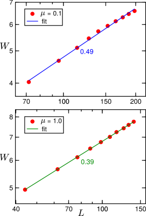
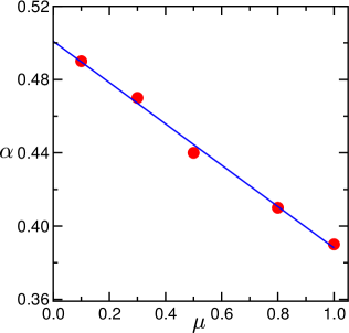
Figure 15: Upper and middle panels: log-log plots of the width $W$ as a function of the length $L$ on the boundary of the sandpile. For different values of $\mu$ the scaling exponent $\alpha$ in Eq. (35) changes. In the lower panel we show the values of $\alpha$ obtained for different values of $\mu$. The exponent $\alpha$ appears to extrapolate to $\alpha=1/2$ for $\mu\to 0$.

The ratio $\cal R$ of $W(L)$ to the height of the sandpile $z_{\rm max}$ will give us an estimate for the importance of the surface fluctuation relative to the size of the sandpile. This ratio is

$${\cal R}=\frac{W(L)}{z_{\rm max}}\approx\frac{2^{\alpha/2}N^{\frac{(\alpha-1)}{2}}}{(\sin 2\phi)^{\alpha/2}\sqrt{\tan\phi}}\ .$$ (37)

We now note that for small values of $\mu$ the angle of repose $\phi\to 0$ and for $\alpha\approx 1/2$,

$${\cal R}\sim N^{-1/4}\phi^{-3/4}\ ,$$ (38)

which becomes of the order of unity when the angle of repose reaches a critical value $\phi_{c}$ where

$$\phi_{c}\sim N^{-1/3}\ .$$ (39)

The meaning of this result is that for a fixed angle of repose there will be a value of $N$ below which scaling is broken since ${\cal R}>1$. For small values of $\phi$ this can be a very large value of $N$.

The same conclusion can be reached from a different point of view. Fluctuations in the surface height will lead to fluctuations in the angle of repose of standard deviation $\delta\phi$ where

$$\delta\phi\sim\frac{W}{L}\sim\left(\frac{L}{\lambda}\right)^{(\alpha-1)}\sim\left(\frac{2N}{\sin 2\phi}\right)^{-1/4}\ .$$ (40)

For small angle of repose the fluctuation in the angle of repose approach the magnitude of the angle of repose itself, when the angle of repose $\phi_{c}$ is of the order $\phi_{c}\sim N^{-1/3}$ as had been previously estimated in Eq. (39). Note that for larger values of $\mu$ similar estimates can be made, but the angle $\phi$ is no longer small, so nonlinear corrections are called for.

V.2 Consequences of breaking of scaling at the bottom

Let us discuss the dip in pressure under the apex of the pile further. To do so we need to focus on the function $\Psi(S,z=h)$. At the bottom when $S\to 1$ one always encounters an edge of the pile with newly added grains that are highly susceptible to height fluctuations. Therefore the form of $\Psi(S\to 1,z=h)$ is no longer given by the form Eq. (10). Since the particles at the edge are mostly subject to gravity rather than the whole weight of a pile on their shoulders, we expect

$$\Psi(1,z=h)=0$$ (41)

to hold. This dramatic change in the form of $\Psi(S,z=h)$ is plotted in Fig. 12. Specifically, while $\Psi(S\rightarrow 0,z=h)\rightarrow 0$ for both scaling and broken scaling solutions, the behavior for $\Psi(S\rightarrow 1,z=h)$ is very different for the scaling and broken scaling principal axis directions. This difference in the functional form of $\Psi$ is probably due to both the interaction of the sandpile with the surface on which it lies, as well as fluctuations of the sandpile surface.

Note also that $\Psi(S\to 1,z=h)$, as can be also seen directly in the simulation results in Figs. 7 and 12, that at some value of $S$, say $S_{m}$, inside the pile, this function has a maximum which is of the order of the value given by the scaling solution Eq. (10). The value of $S_{m}$ can be estimated as follows. Remembering that $S\equiv x\tan\phi/z$ we now use the shift $\Delta x$ towards the maximum and estimate

$$S_{m}=1-\frac{\Delta x\tan\phi}{h}\sim 1-\frac{W}{L}\ ,$$ (42)

where we have used $\Delta x=W\cos\phi$ and $h=L\sin\phi$. Using now Eq. (40) we end up with the estimate

$$S_{m}=1-\left(\frac{2N}{\sin 2\phi}\right)^{-1/4}\ .$$ (43)

In our simulations with $N$ of the order of 1000 $S_{m}\approx 0.8$ in very good agreement with the numerical results.

Accordingly we present in Fig. 16 the positive branch of an anti-symmetric function $\Psi(S,z=h)$ that begins at zero and ends up at zero with a maximum at the expected value of $S_{m}$.

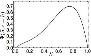
Figure 16: A model function $\Psi(S,z=h)$ which mimics the behavior of the function found in the numerics near the bottom of the pile, as shown in Fig. 12.

This function is simply a fourth order polynomial with coefficients chosen to respect all the wanted properties. The reader should compare this function with “bottom” function shown in the lower panel of Fig. 12. Plugging this function as the constitutive relation into Eqs. (8), (9), we can integrate the equations starting from the outer edge. Solving for the pressure $P\equiv s_{xx}+s_{yy}$ as a function of the angle of repose we get the curves shown in Fig. 17.

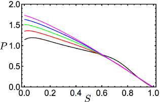
Figure 17: The pressure at the bottom of the pile obtained by integrating the continuum equations starting from the edge. The different curves are for for the same values of $\phi$ as in Fig. 9. For larger angles of repose a dip in the pressure is developing naturally.

Note that we do not need to match two solutions starting from the edge and from the center. The conclusion is that when the angle of repose is small, the pressure is expected to maximize under the apex of the pile. For increasing angles of repose (equivalently increasing $\mu$) there is an increasing tendency for the pressure to dip under the apex with a maximum away from the center. The results indicate that the reason for the dip within the classical continuum theory is actually the breaking of the scaling assumption by the existence of a bottom boundary to the sand-pile. Note that this breaking of scaling is different from the one discussed in the previous subsection where surface fluctuations introduced a typical length-scale.

VI Summary and discussion

In this paper we have examined sandpiles that were grown using a new quasi-static model which allows a detailed computation of the characteristics of the sandpile, including its angle of repose, the stress field, the orientation of the principal axis of the stress etc., all as a function of the coefficient of friction and the system size. We can compare these results with the predictions of a theory based on continuum equilibrium mechanics. As explained, the equations of equilibrium mechanics are under-determined and their solution requires and input of constitute relations. In addition, seeking scaling solutions leads to a very elegant formalism, which appears however to be challenged by the numerical simulations. Note that even when scaling is obeyed, the fact that $\Psi$ is a function of $S$ implies memory in the growth of the sandpile. Further, our sandpiles have stress fields which do not agree with the scaling assumption in all detail, resulting in the function $\Psi$ depending on both $S$ and $z$ and not only on $S$. Fortunately, for larger values of the friction coefficient and for larger system sizes the breaking of scaling is weak in the bulk, allowing an approximate analytic theory which agrees well with the observations. On the other hand, scaling is strongly broken even for large $N$ and for large $\mu$ at the bottom of the pile near the floor. Interestingly enough, when we input the data for $\Psi$ found in the numerics into the analytic theory, we find the often observed dip in the pressure at the center of the pile, without needing to match two piece-wise linear solutions as was necessary in previous publications, 96WCCB ; 97WCC . We propose that our model provides evidence that the dip in the pressure results from the broken scaling solution which presumably is generic due to the special interactions of the particles with the substrate support.

The mechanism proposed here for the appearance of a typical scale that breaks the scaling solutions is not the only one possible. Another interesting proposition was offered in Ref. 01BCLO where the length-scale associated with the bifurcations of the force chains leads to a convective-diffusive equation for the stress field. Solution of this equation predict a dip in the pressure at the bottom of the pile. It is possible that there exist other mechanisms. In fact, one should stress that the particular properties of the numerical model employed in this paper may very well affect the solution. Changing the dissipation mechanism associated with frictional slips, replacing the quasi-static growth of the sandpile with continuous additions of grains before mechanical equilibrium is restored, and other such details, may result in very different profiles of $\Psi(S,z)$. Thus one cannot judge agreement or disagreement with other models 14ZY ; 05GG of the sandpile without comparing the profiles of $\Psi(S,z)$. In the present case discussed above the appearance of non-scaling solutions is strongly supported by the numerics, and the agreement with their shape as discussed in Sect. V.2 gives credence to the mechanism proposed here. It is not impossible that details of the grains shapes, their interactions between themselves and also with the floor may require different approaches to explain the observed characteristics of the sand pile. What should remain invariant is the approach proposed here to expand the solutions near the center of the pile in accordance with the measured profile of $\Psi$ to find what the theory predicts.

- (1) F.H. Hummel and E.J. Finnan, Minutes of Proc. Inst. Civil Eng., Session 1920-1921, Part II, Selected papers 212, 369 (1920).
- (2) B.K. Hough, Trans. ASCE 103, 1414 (1938).
- (3) D.H. Trollope, “The Stability of Wedges of Granular Materials”, PhD thesis, University of Melbourne, 1956.
- (4) J. Smid and J. Novosad, Proc. Powtech D3/V, 1, (1981).
- (5) L. Vanel, D. Howell, D. Clark, R. P. Behringer, and E. Clément, Phys. Rev. E 60, R5040 (1999).
- (6) J. Ai, J.Y. Ooi, J.-F. Chen, J.M. Rotter and Z. Zhong, Mech. of Mat., 66, 160 (2013).
- (7) Q. Zheng and A. Yu, Phys. Rev. Lett. 113, 068001 (2014).
- (8) T. Pöschel and V. Buchholtz, Phys. Rev. Lett. 71, 3963 (1993).
- (9) K. Liffman, D.Y.C. Chan, and B.D. Hughes, Powtech 72 255 (1992); Powtech 78, 263 (1994).
- (10) V. Buchholtz and T. Pöschel, Physica A 202, 390 (1994).
- (11) S. F. Edwards and R.B.S. Oakeshott, Physica D 38, 86 (1989).
- (12) J.P. Bouchaud, M.E. Cates and P. Claudin, J.Phys. I France 5, 639 (1995).
- (13) J.P. Wittmer, P. Claudin, M.E Cates and J.-P. Bouchaud, Nature, 382, 336 (1996).
- (14) J.P. Wittmer, M.E. Cates and P. Claudin, J.Phys. I France 7, 39 (1997).
- (15) Ł. Vanel, D. Howell, D. Clark, R.P. Behringer and E. Clément, Phys. Rev. E 60, R5040 (1999).
- (16) J.-P. Bouchaud, P. Claudin, D. Levine and M. Otto, Eur.Phys. J. E/ 4, 451 (2001).
- (17) J. Fineberg, private communication.
- (18) J.-P. Bouchaud, M.E. Cates, J. Ravi Prakash and S.F. Edwards J. Phys. I France, 4, 1383 (1994) and references therein.
- (19) S. Ostojic, E. Somfai and B. Nienhuis, Nature 439, 828 ( 2006).
- (20) V. Ilyin, N. Makedonska, I. Procaccia, and N. Schupper, Phys. Rev. E 76, 052401 (2007).
- (21) G. Goldenberg and I. Goldhirsch, Nature 435, 188 (2005)