Thermoelectric transport in junctions of Majorana and Dirac channels

Abstract

We investigate the thermoelectric current and heat conductance in a chiral Josephson contact on a surface of a 3D topological insulator, covered with superconducting and magnetic insulator films. The contact consists of two junctions of Majorana and Dirac channels next to two superconductors. Geometric asymmetry results in a supercurrent without a phase bias. The interference of Dirac fermions causes oscillations of the electric and heat currents with an unconventional period $2\Phi_{0}=h/e$ as functions of the Aharonov-Bohm flux. Due to the gapless character of Majorana modes, there is no threshold for the thermoelectric effect and the current-flux relationship is non-sinusoidal. Depending on the magnetic flux, the direction of the electric current can be both from the hot to cold lead and vice versa.

I Introduction

A Majorana fermion is simply the real or imaginary part of a complex fermion. At first sight this implies that no meaningful distinction exists between systems of complex and Majorana fermions. However, it is more practical and much more conventional to use the language of complex fermions for normal metals and many other systems. On the other hand, Majorana fermions provide a natural description for various topological materials. The simplest example is the Kitaev chain Kitaev . Its low-energy degrees of freedom are two Majorana excitations at the chain’s ends. Two-dimensional topological materials bring richer examples of Majorana physics. For example, Majorana edge modes rmp-nonab are expected in several candidates states review-5-2 ; php for the quantum Hall effect at the filling factor $5/2$.

If a Majorana system is in contact with a system of complex fermions then a natural question concerns transformations between the two types of fermions when the systems exchange electrons. The simplest version of that question involves electron tunneling tn1 ; tn2 ; tn3 . A more interesting setting is a Y-junction of Majorana modes that merge into a Dirac quantum channel. Such junctions can be build on a surface of a 3D topological insulator (TI)  FuKane3DTI ; FuKaneMachZehnder .

It has long been known that 1D charge-neutral Majorana fermions can exist as subgap edge modes of 2D chiral $p$-wave topological superconductors qi2011 ; Alicea2012 . An $s$-wave superconductor (SC) can also give rise to such modes in a partially gapped hybrid structure with a superconducting film on a surface of a TI. A splitted film that hosts an SC-insulator-SC interface on top of a 3D TI supports a gapped non-chiral 1D Majorana mode while an SC/ferromagnet junction supports a gapless chiral one ($\chi$MM)  FuKane3DTI ; FuKaneMachZehnder . Recently topological superconductivity and Majorana 1D edge modes were reported in an anomalous quantum Hall insulator/SC heterostructure He and in a single atomic Pb layer on a magnetic Co/Si(111) island Menard .

A magnetic domain wall on top of a TI hosts a chiral Dirac mode ($\chi$DM). Combinations of such domain walls with SC/magnet junctions allow the implementation of novel quantum devices. The simplest example is a Y-junction of Majorana and Dirac modes. Other proposals include the Mach-Zehnder FuKaneMachZehnder ; AkhmerovMachZehnder , Fabry-Pérot LawFabryPerot ; ButtikerFabryPerot , and Hanbury-Brown Twiss HBT quantum interferometers. In our work ShapiroShnirmanMirlin we introduced a 3D TI-based chiral Josephson contact.

The previous work has focused on electric transport in the above devices. In the present paper we extend this line of research to thermoelectric and thermal transport. Our motivation comes from the question about the nonequilibrium state that forms, if two Majorana modes with different temperatures fuse into a Dirac mode. We focus on the setup from Ref. ShapiroShnirmanMirlin, and derive analytical expressions for the thermoelectric and heat currents in the presence of the magnetic field through the normal region. Note that thermal transport between a lead and a 1D Majorana mode has been studied in Ref. thermo-DF, . The case of localized Majorana bound states has been studied in Ref. Ramos, .

Our device is shown in Fig. 1. It can be understood as a Fabry-Pérot interferometer made of four chiral Y-junctions. Each junction converts neutral Majorana fermions into charged Dirac particles. The charge is supplied by a superconductor.

Figure 1: A chiral Josephson junction on a surface of a 3D topological insulator (3D TI). The lines with a single arrow surrounding black superconducting films (SC) stand for gapless Majorana fermion channels $\chi_{r,l}$ and the arrows show chiralities. Superconducting electrodes have different temperatures $T_{l}$ and $T_{r}$. The light and dark gray areas are magnetic insulators (MI) which induce exchange fields of the opposite polarizations and energy gaps $\pm M$. Magnetic domain walls support chiral charged modes $\psi_{a,b}$ marked by double arrows. A magnetic flux $f$ in the $-M$ region induces the Aharonov-Bohm phase $\phi_{AB}=\pi f/\Phi_{0}$.

The device is a relative of a quantum-Hall-based Josephson junction with a gapped superconductor and a quantum Hall bar in the normal region Ostaay ; Zyuzin . In such a structure, the supercurrent is carried by chiral edge states. A recent experimental realization of a quantum Hall junction involved molybdenum-rhenium contacts mediated by a $\mu$m sized graphene bar encapsulated in boron nitride Amet . An important feature, common to our setting and the quantum Hall device, is the spatial separation of electrons and holes in Andreev pairs due to the spatial separation of the chiral transport channels. One consequence of such splitting is a ‘single-electron’ Aharonov-Bohm periodicity in the transport behavior: All transport quantities are periodic in the magnetic flux through the gray region of Fig. 1 with the period $2\Phi_{0}=h/e$. For comparison, S/N/S junctions, based on quantum spin-Hall (or 2D TI) films Tkachov ; LMAY ; Baxevanis or two-channel nanowires Mironov , exhibit even-odd transitions between the $\Phi_{0}$- and $2\Phi_{0}$-periodicities. The heat transport and interference effects in thermally biased 2D TI-based Josephson junctions have been studied in Refs. thermo1-DS, ; thermo2-DS, .

Below we compute the thermal and thermoelectric currents. The time reversal symmetry is broken by the magnetic film. As a consequence, the inevitable geometric asymmetry of the junction results in a nonzero electric current even in the absence of a temperature gradient, a phase difference between superconductors, and an Aharonov-Bohm flux. The thermoelectric effect requires particle-hole asymmetry. This asymmetry is due to the Aharonov-Bohm effect. Our results reveal a significant difference of thermal transport in the setup of Fig. 1 from the threshold-like transport in a conventional S/N/S junction with gapped leads. The thermoelectric current oscillates as a function of the Aharonov-Bohm flux, and, consequently, as a function of the interferometer area. The oscillation amplitude is geometry dependent. We find the maximal current of the order of $eE_{Th}/\hbar\sim e/\tau$, where $E_{Th}$ is the Thouless energy and $\tau$ is the electron travel time through the device, if the temperatures of the leads satisfy $T_{l}\gg E_{Th}\gg T_{r}$ or $T_{r}\gg E_{Th}\gg T_{l}$. The $2\Phi_{0}$-periodic heat conductance oscillates from zero to one half of the heat conductance quantum. The maximum heat conductance agrees with what is expected for a fully transparent junction of chiral Majorana channels Gnezdilov . Note that the experimental measurement of quantized thermal conductance has recently been accomplished in the integer iqhe-thermo and fractional fqhe-thermo quantum Hall effect.

The width $d$ and length $L$ of the normal region, bounded by two counter-propagating charged $\chi$DMs, are much longer than the coherence lengths $\xi$ of the induced superconductivity. Hence, the Thouless energy, proportional to the inverse travel time through the interferometer, is much lower than the superconducting proximity gap and the magnetic exchange gap $E_{Th}\ll\Delta,M$. We assume that the temperatures of the incoming Majorana modes are below those gaps. We will mostly focus on the case of a much higher exchange than superconducting gap $M\gg\Delta$. In this case all contributions to the Josephson current arise from the 1D Dirac channels and do not involve the 2D band between the superconducting leads. Indeed, we expect no contributions to the Josephson effect from the energies $E>M\gg\Delta$. The gray 2D area exhibits insulating behavior for the energies below $M$ and the tunneling through the insulator is suppressed due to its large size $L\gg\xi$. Another assumption is that the superconducting leads are large and have a constant chemical potential which crosses the Dirac point. This means that the DC Josephson effect in this contact is $2\pi$-periodic because the fermion parity is not conserved. The unconventional non-equilibrium $4\pi$-periodic component, predicted in Refs. Kitaev ; Jiang11 ; FuKane ; 1 ; 2 ; Ioselevich for localized zero-energy Majorana bound states Mourik , is suppressed in our device.

Since we only consider 1D physics, we ignore phonons in the bulk. Phonons are not expected to have much effect on the electric current. They do contribute to the thermal conductance. We are only interested in the oscillating contribution from topological modes. One can isolate it experimentally in a setting, where two hot Majorana modes are brought to a cold device.

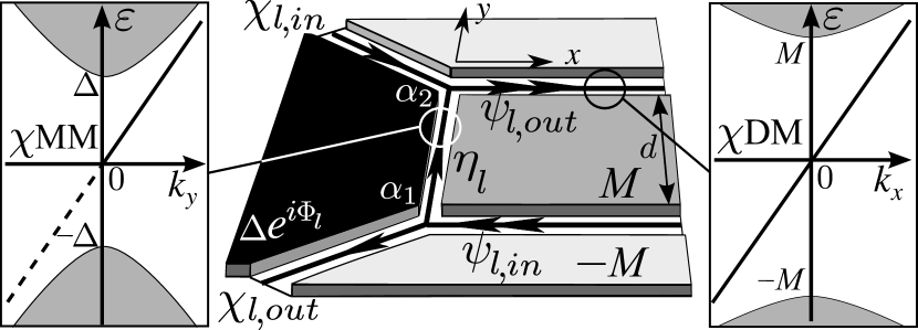
Figure 2: The structure of the chiral Dirac-Majorana 1D contact formed by two Y-junctions. Film of a superconductor with the phase of the order parameter $\Phi_{l}$ and magnetic insulators of the opposite magnetizations induce proximity $\Delta$ and exchange gaps $\pm M$ on the 2D helical surface. The boundaries between the superconductors and magnets support the chiral charged modes $\psi_{in,out}$ and the neutral modes $\chi_{in,out}$ and $\eta_{l}$.

II Dirac and Majorana 1D liquids

The mean-field Hamiltonian of the 2D structure introduced in Fig. 1 reads

$$H=\frac{1}{2}\int dxdy\Psi^{+}h\Psi\ ,\,h=iv\tau_{z}\mathbf{z}\cdot(\boldsymbol{\sigma}\times\boldsymbol{\nabla})+\\ +\tau_{0}\sigma_{z}M(x,y)+(\tau_{+}\Delta(x,y)+\tau_{-}\Delta^{*}(x,y))\sigma_{0},$$ (1)

where $\boldsymbol{\sigma}$ and $\boldsymbol{\tau}$ are the Pauli matrices in the spin and Nambu spaces. The spinor $\Psi=[\psi_{\uparrow},\psi_{\downarrow},\psi_{\downarrow}^{+},-\psi_{\uparrow}^{+}]^{T}$ contains field operators of free electrons and holes on the surface of the topological insulator. The helical states of the 2D surface are described by the Rashba Hamiltonian with the Fermi velocity $v$ and the chemical potential $\mu=0$ crossing the Dirac point. The superconducting $s$-wave pairing potential is given by $\tau_{+}\sigma_{0}\Delta(x,y)$ while the exchange field of the magnetic insulator films is described by $\tau_{0}\sigma_{z}M(x,y)$ term. The black areas of right (left) SC contacts have $\Delta(x,y)=\Delta e^{-i\Phi_{r,l}}$. In the normal region filled with magnetic films the magnetization is perpendicular to the 2D surface and changes its sign: in the light gray regions the induced exchange gap $M(x,y)=M$ and in the dark gray rectangle $M(x,y)=-M$. Both $M$ and $\Delta$ are real.

An effective 1D Hamiltonian of a Majorana mode, like the one marked by single arrow in Fig. 2, was derived by Fu and Kane FuKaneMachZehnder . This derivation is based on a solution of the 2D Bogolyubov-de Gennes equation. Below we review that solution for the mode $\eta$ which connects Y-junctions 1 and 2 in Fig. 2 and propagates along the SC/magnet interface at $x=0$. In the SC region (the $x<0$ half plane), there is an $s$-wave SC pairing potential given by $\Delta(x,y)=\Delta e^{i\Phi_{l}}\theta(-x)$, while at $x>0$ the magnetic film induces the exchange gap $M(x,y)=-M\,\theta(x)$. There exists a 1D solution of the Bogolyubov-de Gennes equation $h\xi_{k_{y}}=\varepsilon_{k_{y}}\xi_{k_{y}}$ such that the wave function decays exponentially in the directions, normal to the SC/magnet interface as $\sim\exp[-|(\theta(x)M-\theta(-x)\Delta)x|/(\hbar v)]$ and is a plane wave with the momentum $k_{y}$ along the boundary. This 1D chiral mode with the dispersion relation

$$\varepsilon_{k_{y}}=-{\rm sign}(M)v{k_{y}}$$ (2)

is nondegenerate within the gap, i.e., for $\varepsilon_{k_{y}}<{\rm min}(\Delta,M)$, but continues to exist also for higher energies. The eigenvectors are self conjugate, $\xi_{k_{y}}=\sigma_{y}\tau_{y}\xi_{-{k_{y}}}^{*}$, which is consistent with the the fact that the field $\Psi$ is self charge conjugate, $\Psi=\sigma_{y}\tau_{y}\Psi^{*}$. Hence, the Bogolyubov quasiparticle operator

$$\eta_{k_{y}}=\int dxdy(\xi_{k_{y}}(x,y))^{\dagger}\cdot\Psi(x,y)$$ (3)

is real, $\eta_{k_{y}}=\eta^{+}_{-k_{y}},$ and describes a chiral Majorana mode.

The normal region with Dirac modes is confined by domain walls where the magnetization sign changes (the horizontal lines marked by double arrows in Fig. 2). To derive the effective 1D Hamiltonian for those modes from the 2D Hamiltonian in the Nambu space (1), we set $\Delta(x,y)=0$ and focus on the mass term $M(x,y)=M\,{\rm sign}(y)$ at $y\approx 0$.

The eigenvalues $\varepsilon_{k_{x}}$ of the Bogolyubov-de Gennes Hamiltonian are now doubly degenerate in contrast to the case of $\chi$MM. We denote two orthogonal degenerate eigenstates as $\zeta_{e,k_{x}}$ and $\zeta_{h,k_{x}}$ and associate them with electrons and holes. Their wave functions are related via the charge conjugation constraint as $\zeta_{h,{k_{x}}}=\sigma_{y}\tau_{y}\zeta_{e,-{k_{x}}}^{*}$. The dispersion relation is the same as for the Majorana channels: $\varepsilon_{k_{x}}=-{\rm sign}(M)v{k_{x}}$. The difference from the neutral mode consists in the existence of two independent excitations of the same energy $\varepsilon_{k_{x}}$ in the Nambu space: an electron of momentum ${k_{x}}$ and a hole of momentum $-{k_{x}}$. In terms of Bogolyubov operators this is the Dirac gapless mode described by a complex field. In the second quantization language, the electron and hole operators are given by

$$\psi_{e,k_{x}}=\int dxdy(\zeta_{e,k_{x}}(x,y))^{\dagger}\cdot\Psi(x,y)\ ,$$ (4)

and

$$\psi_{h,k_{x}}=\int dxdy(\zeta_{h,k_{x}}(x,y))^{\dagger}\cdot\Psi(x,y)\ .$$ (5)

They are not independent since $\psi_{h,k_{x}}=\psi_{e,-k_{x}}^{+}$ due to the charge conjugation constraints for $\Psi(x,y)$ and $\zeta_{e,{k_{x}}},\zeta_{h,{k_{x}}}$. In what follows we do not use $\psi_{h,e}$ and instead introduce the field $\psi_{k_{x}}$ such that $\psi_{e,k_{x}}=\psi_{k_{x}}$ and $\psi_{h,k_{x}}=\psi_{-k_{x}}^{+}$.

At this point we are in the position to write down effective 1D Hamiltonians for free Majorana and Dirac particles. The secondary quantized $\Psi$-operators of these 1D modes are:

$$\Psi_{M}(x,y)=\int\frac{dk_{y}}{2\pi}\xi_{k_{y}}(x,y)\eta_{k_{y}}$$ (6)

for $\chi$MM and

$$\Psi_{D}(x,y)=\int\frac{dk_{x}}{2\pi}\left(\zeta_{e,k_{x}}(x,y)\psi_{k_{x}}+\zeta_{h,k_{x}}(x,y)\psi_{-k_{x}}^{+}\right)$$ (7)

for $\chi$DM. Integrating out the $y$ coordinate in the Bogolyubov-de Gennes Hamiltonian yields the effective Hamiltonians of the Majorana modes

$$H_{M}={\rm sign}(M)\frac{iv}{2}\int\!\eta(y)\partial_{y}\eta(y)dy$$ (8)

and the Dirac modes

$$H_{D}={\rm sign}(M)iv\int\!\psi^{+}(x)\partial_{x}\psi(x)dx,$$ (9)

where we introduced the 1D operators

$$\eta(y)=\eta^{+}(y)=\int\frac{d{k_{y}}}{2\pi}\eta_{k_{y}}e^{i{k_{y}}y}$$ (10)

and

$$\psi(x)=\int\frac{d{k_{x}}}{2\pi}\psi_{k_{x}}e^{i{k_{x}}x},$$ (11)

which describe coherent propagation of neutral and charged fermions through 1D guiding channels with the Fermi velocity $v$. For $M>0$ the chiralities of the 1D modes are shown by the arrows in Figs. 1 and 2. The factor $1/2$ in the Majorana Hamiltonian $H_{M}$ reflects the fact that the negative and positive energy excitations in the $\chi$MM are not independent. In other words, the lower branch of the dispersion $\varepsilon_{k_{y}}=-{\rm sign}(M)v{k_{y}}$ at ${k_{y}}<0$ is redundant (it is shown as a dashed line in the left inset of Fig. 2). The coefficient $1/2$ implies that a neutral Majorana fermion carries only a half of the heat current of a Dirac mode at the same temperature so that the ballistic heat conductance $G_{0}$ of a single $\chi$MM is one half of the heat conductance quantum:

$$G_{0}=\frac{1}{2}\frac{\pi^{2}k_{\rm B}^{2}T}{3h},$$ (12)

where $T$ is the temperature.

III Scattering in a Majorana-Dirac contact

The normal region includes a rectangular magnetic film (dark gray area in Fig. 1) of the length $L$ and the width $d$. $L$ and $d$ exceed significantly both the SC and magnetic coherence lengths $d,L\gg\hbar v/\Delta,\hbar v/M$. Four Y-junctions are in the corners of the film. A single Y-junction is formed by two Majorana and one Dirac channels (Fig. 2). The angles between the channels as well as other microscopic details are not necessarily the same in different Y-junctions.

We start with the calculation of the scattering matrix describing two nonidentical Y-junctions shown in Fig. 2 (see ShapiroShnirmanMirlin ). This scattering matrix describes the coupling between $\chi$MMs on the SC/magnet interfaces and two 1D Dirac modes. Specifically, it provides a relation between the operators of incoming and outgoing electrons and holes $\psi_{in,out},\psi_{in,out}^{+}$ of $\chi$DM (horizontal lines marked by double arrow) and $\chi_{in,out}$ of semi-infinite neutral $\chi$MMs (lines marked by single arrow). The 1D modes, described by the wave functions $\xi$ and $\zeta_{e,h}$ are spin-nondegenerate and have in-plane spin textures. Hence, the conversion between Majorana and Dirac modes in Y-junctions is accompanied by spin rotation. Thus, scattering in a Y-junction involves a geometric Berry phase, which is encoded in the phase $\alpha$ below. The calculation of $\alpha$ for a given geometry is straightforward.

Scattering in the upper and lower Y-junctions in Fig. 2 is described by the $S_{out}$ and $S_{in}$ matrices which were found in Refs. AkhmerovMachZehnder, ; FuKaneMachZehnder,

$$\begin{bmatrix}\eta_{l,out}\\ \\ \chi_{l,out}\end{bmatrix}=S_{in,\alpha_{1}}\begin{bmatrix}\psi_{l,in}\\ \\ \psi_{l,in}^{+}\end{bmatrix},\,\,\,\begin{bmatrix}\psi_{l,out}\\ \\ \psi_{l,out}^{+}\end{bmatrix}=S_{out,\alpha_{2}}\begin{bmatrix}\eta_{l,in}\\ \\ \chi_{l,in}\end{bmatrix}$$ (13)

Note that the operators in (13) correspond to the incoming and outgoing scattering states rather than to free plane waves of (3), (4), and (5) Blanter .

Let us assume first that $\Phi_{l}=0$ in the electrode. A non-zero $\Phi_{l}$ will be included in a final expression for the $S$-matrix by means of a gauge transformation of Dirac $\psi$-operators. The matrix $S_{in,\alpha_{1}}$ involves the phase difference $\alpha_{1}$ between an electron and hole converting into two Majorana fermions. The matrix $S_{out,\alpha_{2}}$ involves a phase $\alpha_{2}$ accumulated under merging two Majoranas into a Dirac fermion. The structure of $S_{out}$ is related to that of $S_{in}$ by a time-reversal transformation AkhmerovMachZehnder : $S_{out}=S_{in}^{T}.$ The expression for the $S_{in}$-matrix of the lower Y-junction is

$$\quad S_{in,\alpha_{1}}=\begin{bmatrix}1/\sqrt{2}&&1/\sqrt{2}\\ \\ i/\sqrt{2}&&-i/\sqrt{2}\end{bmatrix}\begin{bmatrix}e^{i\alpha_{1}}&&0\\ \\ 0&&e^{-i\alpha_{1}}\end{bmatrix}.$$ (14)

Note that whereas the phase $\alpha_{1}$ can be easily gauged out if the Y-junction is considered on its own, it becomes important once several Y-junctions are combined into a circuit.

In Ref. ShapiroShnirmanMirlin the symmetry of four Y-junctions ($\alpha_{i}=\alpha$) was assumed. In this paper we consider an arbitrary set of the phases $\alpha_{i}$. We will see that this modifies the current-phase relation in such a way that a nonzero current may flow at a zero external phase bias $\Phi$, like in Josephson $\varphi$-junction devices Buzdin ; Goldobin ; Sickinger .

We proceed by matching the Majorana operators $\eta_{l,in}$ and $\eta_{l,out}$ at a given energy $\varepsilon$ as $\eta_{l,in,\varepsilon}=e^{ik_{\varepsilon}}\eta_{l,out,\varepsilon}$. The dynamic phase $k_{\varepsilon}=\varepsilon d/v$ is accumulated by a Majorana excitation during the propagation from the lower to upper Y-junctions, separated by the distance $d$. The full $S_{\alpha_{1},\alpha_{2}}$-matrix of the contact, acting on $(\psi_{in,\varepsilon},\ \chi_{in,\varepsilon},\ \psi^{+}_{in,-\varepsilon})^{T}$, can be found after the exclusion of $\eta$ from Eqs. (13) and is defined by the equation

$$\begin{bmatrix}\psi_{l,out,\varepsilon}\\ \\ \chi_{l,out,\varepsilon}\\ \\ \psi^{+}_{l,out,-\varepsilon}\\ \end{bmatrix}=\\ =\begin{bmatrix}\frac{1}{2}e^{ik_{\varepsilon}+i(\text{$\alpha_{1}$}+\text{$\alpha_{2}$})}&\frac{ie^{i\text{$\alpha_{2}$}}}{\sqrt{2}}&\frac{1}{2}e^{ik_{\varepsilon}-i(\text{$\alpha_{1}$}-\text{$\alpha_{2}$})}\\ \\ \frac{ie^{i\text{$\alpha_{1}$}}}{\sqrt{2}}&0&-\frac{ie^{-i\text{$\alpha_{1}$}}}{\sqrt{2}}\\ \\ \frac{1}{2}e^{ik_{\varepsilon}+i(\text{$\alpha_{1}$}-\text{$\alpha_{2}$})}&-\frac{ie^{-i\text{$\alpha_{2}$}}}{\sqrt{2}}&\frac{1}{2}e^{ik_{\varepsilon}-i(\text{$\alpha_{1}$}+\text{$\alpha_{2}$})}\\ \end{bmatrix}\begin{bmatrix}\psi_{l,in,\varepsilon}\\ \\ \chi_{l,in,\varepsilon}\\ \\ \psi^{+}_{l,in,-\varepsilon}\\ \end{bmatrix}.$$ (15)

To account for a non-zero SC phase $\Phi_{SC}$ of an electrode (colored black in Figure 2), we employ the transformation $\psi\to e^{i\Phi_{SC}/2}\psi$. For the left contact in Fig. 1 this yields

$$S_{l}=C(-\Phi_{l})S(\alpha_{1},\alpha_{2})C(\Phi_{l}),$$ (16)

while for the scattering matrix for the right contact it gives

$$S_{r}=C^{-1}(\Phi_{r})S(\alpha_{3},\alpha_{4})C(\Phi_{r}).$$ (17)

Here we have introduced an auxiliary matrix

$$C(\Phi_{SC})=\begin{bmatrix}e^{i\Phi_{SC}}&0&0\\ \\ 0&1&0\\ \\ 0&0&e^{-i\Phi_{SC}}\\ \end{bmatrix}.$$ (18)

The above $S_{l,r}$-matrices describe partial Andreev reflection in spinless 1D Dirac channels and the creation of excitations in neutral Majorana modes. The Andreev part of this process is accompanied by a Cooper pair absorption in an SC electrode.

We transform the $S_{l,r}$-matrices acting on $\psi_{l,in},\psi_{l,out}$ ($\psi_{r,in},\psi_{r,out}$) on the left (right) ends of the Dirac channels into new matrices $\tilde{S}_{l,r}$, acting on the operators $\psi_{a},\psi_{b}$ in the geometric centers of the 1D channels. The $S$ and $\tilde{S}$ operators are related by a phase shift by the sum of the dynamical phase $\frac{\varepsilon L}{2\hbar v}$, accumulated by an electron of energy $\varepsilon$ over the distance $L/2$, and an Aharonov-Bohm phase. For the upper $a$-arm the relation of the scattering matrices can be deduced from the equation

$$\psi_{a,\varepsilon}=e^{i\frac{\varepsilon L}{2\hbar v}+i\phi_{AB}/4}\psi_{l,out,\varepsilon}.$$ (19)

We assume here that the same Aharonov-Bohm phases are accumulated on each portion of the Dirac channels of the same length. The scattering matrices, acting on the $\psi$-operators in the centers of the channels, take the form

$$\tilde{S}_{l,r}=C\left(\frac{\phi_{AB}}{4}\right)D\left(\frac{\varepsilon L}{2v}\right)S_{l,r}D\left(\frac{\varepsilon L}{2v}\right)C\left(\frac{\phi_{AB}}{4}\right),$$ (20)

where $\phi_{AB}$ is the total Aharonov-Bohm phase. The dynamical phases are encoded in (20) via the matrix

$$D\left(\frac{\varepsilon L}{2\hbar v}\right)=\begin{bmatrix}e^{i\frac{\varepsilon L}{2\hbar v}}&0&0\\ \\ 0&1&0\\ \\ 0&0&e^{i\frac{\varepsilon L}{2\hbar v}}\\ \end{bmatrix}.$$ (21)

The difference of the above expression from the $C$-matrix is that the first and third diagonal components coincide: the dynamical phases are equal for an electron of the energy $\varepsilon$ and a hole of the energy $-\varepsilon$. We can exclude $\alpha_{i}$ from the diagonal terms of the $S$-matrices by redefining the superconducting phase bias $\Phi$ and the Aharonov-Bohm phase $\phi_{AB}$. To do that we introduce the phases

$$\phi_{l}=\frac{\alpha_{1}+\alpha_{2}}{2},\quad\phi_{r}=\frac{\alpha_{3}+\alpha_{4}}{2}$$ (22)

and

$$\varphi_{0}=\frac{\Phi_{l}+\Phi_{r}}{2}.$$ (23)

We can always shift both superconducting phases by the same constant. It will be convenient to shift them so that

$$\varphi_{0}=\frac{\alpha_{2}-\alpha_{1}+\alpha_{4}-\alpha_{3}}{4}.$$ (24)

With this choice we find

$$S_{l}=C\left(\phi_{l}-(\Phi+\varphi)/2\right)S_{0}C\left(\phi_{l}+(\Phi+\varphi)/2\right)$$ (25)

and

$$S_{r}=C\left(\phi_{r}+(\Phi+\varphi)/2\right)S_{0}C\left(\phi_{r}-(\Phi+\varphi)/2\right),$$ (26)

where $S_{0}\equiv S_{\alpha_{1}=\alpha_{2}=0}$ (15),

$$\Phi=\Phi_{l}-\Phi_{r}$$

is the SC phase bias, and the phase shift

$$\varphi=\frac{1}{2}(\alpha_{1}-\alpha_{2}-\alpha_{3}+\alpha_{4}).$$ (27)

It follows from this representation of $S_{l,r}$ and $\tilde{S}_{l,r}$ that the superconducting phase cannot be gauged out by the Aharonov-Bohm phase. We also observe that $\phi_{l,r}$ and $\phi_{AB}$ enter the $C$-matrices in the same way, and hence, $\phi_{l,r}$ can be gauged out by redefining the total Aharonov-Bohm phase as

$$\phi_{AB}\to\phi_{AB}+2(\phi_{l}+\phi_{r})=\sum\limits_{i}^{4}\alpha_{i}+\phi_{AB}.$$ (28)

IV Josephson current

In our formalism the operators of Dirac fermions are expressed as linear combinations of uncorrelated field operators $\chi_{l}\equiv\chi_{l,in}$ and $\chi_{r}\equiv\chi_{r,in}$ of incident Majorana modes. The latter are characterized by the Fermi distribution functions

$$n_{l,r}(\varepsilon)=\frac{1}{2}\left(1-\tanh\frac{\varepsilon}{2T_{l,r}}\right),$$ (29)

i.e.,

$$\langle\chi_{\varepsilon,i}^{\dagger}\chi_{\varepsilon,j}^{\phantom{{\dagger}}}\rangle=v^{-1}\delta_{i,j}n_{i}(\varepsilon),$$ (30)

where the Fourier transformed operators

$$\chi_{\varepsilon,i}=\chi_{-\varepsilon,i}^{\dagger}=\int\chi_{i}(t)e^{i\varepsilon t}dt,$$ (31)

and the index $i=l,r$ stands for the left and right incident modes and $v^{-1}$ is the density of states in the $\chi$MM channels. We assume $k_{\rm B}=1$ everywhere and recover it in the final expressions. The linear spectrum of 1D Dirac modes means that the chiral current is proportional to the charge density $j_{a,b}=-ev\rho_{a,b}$ and, hence, the current $j$ is given by the integral over energies

$$j=\int\frac{d\varepsilon}{2\pi\hbar}(-ev)(\langle\psi_{a,\varepsilon}^{+}\psi_{a,\varepsilon}\rangle-\langle\psi_{b,\varepsilon}^{+}\psi_{b,\varepsilon}\rangle)\ .$$ (32)

Here $\psi_{a,\varepsilon}$ and $\psi_{b,\varepsilon}$ are the electron operators in the centers of the Dirac channels and the positive direction of the current is defined from the left to the right.

The $S$-matrices are used to express the Dirac fermion operators in Eq. (32) in terms of the incoming Majorana modes

$$\psi_{a,\varepsilon}=\frac{i\sqrt{2}e^{\frac{1}{4}i(\frac{2L\varepsilon}{v}+\phi-\Phi-\varphi)}}{1+2e^{i\phi}\cos(\Phi+\varphi)+e^{2i\phi}-4e^{i(\phi-\varphi_{\varepsilon})}}\times\\ \left[\left(1+e^{i(\Phi+\varphi+\phi)}-2e^{i(\phi-\varphi_{\varepsilon})}\right)\chi_{l}-\right.\\ \left.-2ie^{i\phi-i\frac{1}{2}\varphi_{\varepsilon}}\sin\left(\frac{\Phi+\varphi+\phi}{2}\right)\chi_{r}\right]$$ (33)

with

$$\phi=\phi_{AB}+\sum\limits_{i}\alpha_{i}.$$ (34)

Due to the symmetry between the $a$ and $b$ arms we get a similar expression for $\psi_{b}$ with $\Phi\to-\Phi,\varphi\to-\varphi$ and the interchanged $\chi_{l}$ and $\chi_{r}$. This expression for Dirac operators is a straightforward generalization of that from Ref. ShapiroShnirmanMirlin, to our asymmetric setup: (i) the sum of the phases $\alpha_{i}$ shifts the total Aharonov-Bohm phase (34) and (ii) the phase $\varphi$, introduced in (27), shifts the external superconducting phase bias $\Phi$.

With the use of the expressions for Dirac operators in N-region (33) we obtain that the current can be represented as

$$j=j_{t}+j_{\Phi}$$ (35)

where $j_{t}$ is induced by the temperature gradient and $j_{\Phi}$ generalizes the Josephson current from Ref. ShapiroShnirmanMirlin, to a two-temperature situation. The two contributions read as

$$j_{t}=\int\frac{d\varepsilon}{2\pi\hbar}(-e)\frac{n_{l}(\varepsilon)-n_{r}(\varepsilon)}{2}J_{t,\varepsilon},$$ (36)

and

$$j_{\Phi}=\int\frac{d\varepsilon}{2\pi\hbar}(-e)\frac{n_{l}(\varepsilon)+n_{r}(\varepsilon)}{2}J_{\varepsilon}.$$ (37)

Thermoelectric part (36) is given by a rapidly convergent integral due to the factor $(n_{l}-n_{r})$. If $T_{l}=T_{r}$ then $j_{t}=0$ and the total current (35) is given by the Josephson term $j_{\Phi}$. We calculate $j_{\Phi}$ in this section and analyze $j_{t}$ in the next one.

The spectral current $J_{\varepsilon}$, entering into $j_{\Phi}$, reads

$$J_{\varepsilon}=\frac{\sin\varphi_{\varepsilon}\sin(\Phi+\varphi)}{1+\left(\frac{\cos\phi+\cos(\Phi+\varphi)}{2}\right)^{2}-(\cos(\Phi+\varphi)+\cos\phi)\cos\varphi_{\varepsilon}}\ ,$$ (38)

with $\varphi_{\varepsilon}=\varepsilon/E_{Th}$ being the dynamical phase, accumulated by an excitation of the energy $\varepsilon$ on the closed path that connects all four Y-junctions. Note that the Josephson term (37) does not converge at high $\varepsilon$ and a regularization is needed. Indeed, the spectral current (38) depends periodically on the energy, due to the 1D nature of the chiral modes carrying the current. On physical grounds we expect this dependency to be replaced by a slowly decaying (and oscillating) one, once the energy $\varepsilon$ reaches the lowest border of the 2D continuum, ${\rm min}(\Delta,M)\gg E_{Th}$. We, thus, smoothly cut off the integration in (37) at $\varepsilon\gg E_{Th}$ which leads to the following current-phase relationship for equal $T_{l}=T_{r}=T$

$$j_{\Phi}=4\pi{\frac{ek_{\rm B}T}{h}}\sin(\Phi+\varphi)\times\\ \sum\limits_{n=0}^{\infty}\frac{1}{2\exp\left(\pi\frac{k_{\rm B}T(1+2n)}{E_{Th}}\right)-\cos\phi-\cos(\Phi+\varphi)}.$$ (39)

The phase $\phi$ shifts $h/e$-periodic pattern of critical current-flux oscillations, while $\varphi$ results into non-zero Josephson current without phase bias. The result for different temperatures $T_{l}\neq T_{r}$ equals half the sum of the two expressions (39) taken at $T=T_{l}$ and at $T=T_{r}$ respectively.

To further support the validity of this the regularization procedure based on smooth cutoff, we can perform the derivation in a slightly different way that leads to the same result. Specifically, this alternative – but equivalent – regularization procedure amounts to subtracting and adding a high-temperature Josephson current at $T_{l}=T_{r}\gg E_{Th}$. The difference of the Josephson current and the counter-term converges. At the same time, the counter-term is expected to be negligible on physical grounds. Indeed, the Josephson effect is possible due to the particle-hole coherence between the two Dirac channels. Such coherence extends to the length scales of the order of the thermal length $hv/(k_{\rm B}T)$. For $T\gg E_{Th}$ the thermal length is much shorter than the distance $L$ between the superconductors. Thus, the high-temperature Josephson effect is suppressed. This agrees with the results for S/N/S structures, where the normal region is a long quantum wire Winkelholz ; Maslov ; Fazio ; Dubos ; Levchenko . We emphasize once again that the convergence subtlety discussed here relates to the Josephson current only. The thermoelectric and the heat currents discussed below are given by convergent integrals.

V Thermoelectric current

Below we focus on the thermoelectric effect. Thus, we take $T_{l}\neq T_{r}$ and set the SC phase bias $\Phi=-\varphi$ so that the Josephson current $j_{\Phi}=0$ in (35). Recall that we have redefined the Aharonov-Bohm phase $\phi$ in Eq. (34). We investigate the current $j_{t}$ as a function of two temperatures, $T_{l,r}$, and of $\phi$. We use the scattering matrices to express the $\psi_{a,\varepsilon}$-operator at $\Phi=-\varphi$ in the center of the upper Dirac channel as We use the expression (33) for $\psi_{a,\varepsilon}$-operator at $\Phi=-\varphi$ in the center of the upper Dirac channel

$$\psi_{a,\varepsilon}=i\sqrt{2}e^{\frac{1}{4}i\left(\frac{2L\varepsilon}{v}+\phi\right)}\\ \frac{\left(e^{i\varphi_{\varepsilon}}+e^{i\left(\varphi_{\varepsilon}+\phi\right)}-2e^{i\phi}\right)\chi_{l}-\left(e^{i\phi}-1\right)e^{\frac{1}{2}i\left(\varphi_{\varepsilon}+\phi\right)}\chi_{r}}{e^{i\varphi_{\varepsilon}}(1+e^{i\phi})^{2}-4e^{i\phi}}.$$ (40)

The $\psi_{b}$ is given by the interchanged $\chi_{l}$ and $\chi_{r}$ for the rectangular geometry of the N-region.

The above operator relations (40) allow the calculation of the dimensionless spectral current $J_{t,\varepsilon}$ entering $j_{t}$, Eq. (36):

$$J_{t,\varepsilon}=\frac{(1+\cos\phi)(1-\cos\varphi_{\varepsilon})-\sin\phi\sin\varphi_{\varepsilon}}{1+\left(\frac{1+\cos\phi}{2}\right)^{2}-(1+\cos\phi)\cos\varphi_{\varepsilon}}.$$ (41)

The term $(1+\cos\phi)(1-\cos\varphi_{\varepsilon})$ in (41) is an even function of $\varepsilon$ and does not contribute to the integral (36) which is evaluated by means of the summation over the residues of $\tanh\left(\varepsilon/(2T_{l,r})\right)$. Finally, for arbitrary temperatures and $\phi$ we obtain an expression for the thermoelectric current

$$j_{t}=\frac{k_{\rm B}e}{\hbar}\sin\phi\sum\limits_{n=0}\left(\frac{T_{r}}{2\exp\left(\frac{\pi k_{\rm B}T_{r}(1+2n)}{E_{Th}}\right)-1-\cos\phi}\right.\\ \left.-\frac{T_{l}}{2\exp\left(\frac{\pi k_{\rm B}T_{l}(1+2n)}{E_{Th}}\right)-1-\cos\phi}\right).$$ (42)

We focus on the regime of $T_{l}\gg E_{Th}\gg T_{r}$ or $T_{r}\gg E_{Th}\gg T_{l}$. We expect the maximal current to be achieved in that region (see the solid curve in Fig. 3). In those cases the terms in the sum (42) with the higher of the two temperatures are exponentially small. The sum of the remaining terms reduces to the integral $T\sum\limits\to E_{Th}\int dx$, where $x=T/E_{Th}$ and $T$ is the smaller of $T_{r}$ and $T_{l}$. The integral is proportional to $eE_{Th}/\hbar$:

$$j_{t,max}={\rm sign}(T_{l}-T_{r})\left.\frac{eE_{Th}}{2\pi\hbar}\tan\frac{\phi}{2}\,\ln\frac{2}{1-\cos\phi}\right..$$ (43)

Note the divergent derivative $\partial_{\phi}j_{max}(\phi)$ at $\phi=2\pi n$.

Figure 3: The thermoelectric current $j_{t}(\phi)$ and the heat current $j_{h}(\phi)$ as functions of the flux $\phi$ at $T_{l}\gg E_{Th}\gg T_{r}$.

In the high temperature regime, where $T_{l},T_{r}\gg E_{Th}$, the thermoelectric current is exponentially suppressed and exhibits a sinusoidal dependence on $\phi$

$$j=\frac{k_{\rm B}e}{2\hbar}\sin\phi\left(T_{r}e^{-\pi T_{r}/E_{Th}}-T_{l}e^{-\pi T_{l}/E_{Th}}\right).$$ (44)

Similar to the electric current, the thermoelectric current decays exponentially at $k_{\rm B}T_{l,r}\gg E_{Th}$. This is the limit where the thermal length becomes much less than the interferometer size.

We next briefly address a general situation with nonzero Josephson and thermoelectric currents. We derive from (33) that $J_{t,\varepsilon}$, entering the thermoelectric contribution (36), reads for arbitrary temperatures, superconducting phases, and Aharonov-Bohm phases as

$$J_{t,\varepsilon}(\Phi)=\\ =\frac{1+(\cos\phi-\cos\varphi_{\varepsilon})\cos(\Phi+\varphi)-\cos(\phi-\varphi_{\varepsilon})}{1+\left(\frac{\cos\phi+\cos(\Phi+\varphi)}{2}\right)^{2}-(\cos(\Phi+\varphi)+\cos\phi)\cos\varphi_{\varepsilon}}\ ,$$ (45)

Comparing the above equation (45) with $J_{\varepsilon}$ from (37) we relate the thermoelectric current $j_{t}$ and the Josephson currents $j_{\Phi}(T_{r,l})$ (39):

$$j_{t}=\frac{\sin\phi}{2\sin(\Phi+\varphi)}\left(j_{\Phi}(T_{r})-j_{\Phi}(T_{l})\right).$$ (46)

At $T_{r}\neq T_{l}$, the Josephson current reads

$$j_{\Phi}=\frac{1}{2}\left(j_{\Phi}(T_{r})+j_{\Phi}(T_{l})\right).$$ (47)

Fig. (4) shows the bias dependencies of the thermoelectric and Josephson currents at the Aharonov-Bohm phase $\phi=\pi/3$ in three temperature domains: (a) $T_{r,l}<E_{Th}$, (b) $T_{l}>E_{Th}>T_{r}$ and (c) $T_{r,l}>E_{Th}$. In regime (a) the Josephson part is maximal, but the thermoelectric effect is suppressed. In (b,c) the thermal and Josephson parts are of the same orders of magnitude, $j_{t}\sim j_{\Phi}$. From (c) we see that the dependence of $j_{t}$ on $\Phi$ vanishes at high temperatures.

Below we compute the bias phase $\Phi^{*}$ which results in zero total current

$$j(\Phi^{*},T_{r},T_{l})=0.$$ (48)

This value of the phase can be seen as an analogue of thermovoltage in the Josephson effect. In this regime (48), where the Josephson and thermal currents compensate each other, one finds

$$j_{\Phi^{*}}=-j_{t}.$$ (49)

From (46,47) and (49) we obtain an equation on $\Phi^{*}$

$$\sin(\Phi^{*}+\varphi)=\frac{j_{\Phi^{*}}(T_{l})-j_{\Phi^{*}}(T_{r})}{j_{\Phi^{*}}(T_{l})+j_{\Phi^{*}}(T_{r})}\sin\phi,$$ (50)

where $j_{\Phi}$ was introduced in (39).

The relation between $\Phi^{*}$ and the temperature gradient $\Delta T=T_{r}-T_{l}$ is nonlinear. Let us consider several limiting cases of (50) and their solutions. The first one is the high-temperature limit with $T_{r},T_{l}\gg E_{Th}$. In this case the currents are

$$j_{\Phi}(T_{l,r})=2\pi\frac{ek_{\rm B}T_{l,r}}{h}\exp\left(-\frac{\pi T_{l,r}}{E_{Th}}\right)\sin(\Phi+\varphi),$$ (51)

and the solution for $\Phi^{*}$ reads

$$\Phi^{*}=\arcsin\left(\sin\phi\tanh\frac{\pi(T_{r}-T_{l})}{2E_{Th}}\right)-\varphi$$ (52)

In the limits of $T_{l}\gg E_{Th}\gg T_{r}$ or $T_{r}\gg E_{Th}\gg T_{l}$, one of the currents in (50) is temperature-independent and is given by $j_{\Phi}\propto E_{Th}$, while the other is exponentially suppressed as in (51). The result is

$$\Phi^{*}=\phi\ {\rm sign}(T_{r}-T_{l})-\varphi.$$ (53)

In the low-temperature limit $T_{r},T_{l}\ll E_{Th}$, for small gradients $\Delta T\ll T\ll E_{Th}$, we obtain that

$$\Phi^{*}=\frac{\Delta T}{3}\frac{\pi^{2}k_{\rm B}^{2}T}{E^{2}_{Th}}\frac{(1+\cos\phi)\sin\phi}{(1-\cos\phi)^{2}\ln\frac{2}{1-\cos\phi}}-\varphi$$ (54)

with $\Delta T=T_{r}-T_{l}.$

Figure 4: The thermoelectric $j_{t}(\Phi)$ and Josephson $j_{\Phi}(\Phi)$ parts of the current as functions of the superconducting phase $\Phi$, with the phase $\varphi$ set to zero. The Aharonov-Bohm phase is $\phi=\pi/3$.

VI Heat current

The energy current at $\Phi=-\varphi$ is defined analogously to the thermoelectric one (36) with the replacement of the electron charge by the energy $(-e)\to\varepsilon$:

$$j_{h}=\int\frac{d\varepsilon}{2\pi\hbar}\varepsilon\frac{n_{l}(\varepsilon)-n_{r}(\varepsilon)}{2}J_{t,\varepsilon}.$$ (55)

The part in $J_{t,\varepsilon}$ (41) which is proportional to $\sin\phi\sin\varphi_{\varepsilon}$ and contributes to $j_{t}$ does not contribute to $j_{h}$ while the term $\sim(1+\cos\phi)(1-\cos\varphi_{\varepsilon})$ from $J_{t,\varepsilon}$ does contribute to the energy current. The result of the integration at an arbitrary temperatures reads

$$j_{h}=\frac{\pi^{2}k_{\rm B}^{2}}{6h}\frac{1+\cos\phi}{3+\cos\phi}(T_{l}^{2}-T_{r}^{2})+\pi^{2}\frac{1-\cos^{2}\phi}{3+\cos\phi}\times\\ \!\!\!\sum\limits_{n=0}^{\infty}\!\left(\frac{k_{\rm B}^{2}T_{r}^{2}(2n+1)/h}{\exp\left[\frac{\pi k_{\rm B}T_{r}(1+2n)}{E_{Th}}\right]-\cos^{2}(\phi/2)}-(T_{r}{\to}T_{l})\!\right).$$ (56)

The first term in (56) gives a ballistic contribution to the heat conductance modulated by $\phi$. The heat current is $h/e$-periodic like the electric current but the energy current has always the same sing in contrast to the electric current $j_{t}$. In the limit of $T_{l}\gg E_{Th}\gg T_{r}$ the amplitude of the heat current oscillations is maximal:

$$j_{h,max}=\frac{\pi^{2}k_{\rm B}^{2}T_{l}^{2}}{6h}\frac{1+\cos\phi}{3+\cos\phi}\\ +\frac{E_{Th}^{2}}{h}\frac{1-\cos\phi}{3+\cos\phi}{\rm Li}_{2}(\cos^{2}(\phi/2)),$$ (57)

where ${\rm Li}_{2}(z)$ is the polylogarithmic function ${\rm Li}_{n}(z)=\sum\limits_{k=1}^{\infty}z^{k}/k^{n}.$ The dependence of $j_{h}(\phi)$ on the flux is shown in Fig. 3 as a dashed curve. Depending on Aharonov-Bohm phase the thermoelectric and heat currents can flow in opposite ($0<\phi<\pi$) or in the same ($\pi<\phi<2\pi$) directions. One sees that the heat current $j_{h}$ is maximal at $\phi=0$ with the value

$$j_{h}(0)=\frac{\pi^{2}k_{\rm B}^{2}T_{l}^{2}}{12h}(T_{l}^{2}-T_{r}^{2}),$$ (58)

which is half of the ballistic heat current of complex 1D fermions. The heat current is zero at $\phi=(2n+1)\pi$. The origin of the zeros of $j_{h}$ becomes transparent after one represents the Dirac $\psi$-operators in the normal region using a Majorana basis $\gamma_{1}$, $\gamma_{2}$:

$$\gamma_{1}=(\psi+\psi^{+})/\sqrt{2},\quad\gamma_{2}=-i(\psi^{+}-\psi)/\sqrt{2}.$$ (59)

The total phase $\phi=\phi_{AB}+\sum\limits_{i}^{4}\alpha_{i}=\pi$ can be interpreted as the sum of a zero Aharonov-Bohm phase and a set of redefined $\alpha_{i}$’s, for instance, with $\alpha_{l}=\alpha_{1}=\alpha_{2}=\pi/2$ and $\alpha_{r}=\alpha_{3}=\alpha_{4}=0$. The scattering between $\chi,\gamma_{1}$ and $\gamma_{2}$ for such contacts with equal phases $\alpha$ of Y-junctions was found in Ref. ShapiroShnirmanMirlin, , Eq. (37)

$$\begin{bmatrix}\gamma_{1,out}\\ \\ \chi_{{}_{\beta},out}\\ \\ \gamma_{2,out}\end{bmatrix}=\begin{bmatrix}\cos^{2}\alpha_{\beta}&&-\sin\alpha_{\beta}&&-\frac{\sin 2\alpha_{\beta}}{2}\\ \\ -\sin\alpha_{\beta}&&0&&-\cos\alpha_{\beta}\\ \\ \frac{\sin 2\alpha_{\beta}}{2}&&\cos\alpha&&-\sin^{2}\alpha_{\beta}\end{bmatrix}\begin{bmatrix}\gamma_{1,in}\\ \\ \chi_{{}_{\beta},in}\\ \\ \gamma_{2,in}\end{bmatrix}$$ (60)

with the index $\beta=l,r$. From this representation of the scattering matrices for the left and right contacts, i.e. for $\alpha_{l}=\pi/2$ and $\alpha_{r}=0$, we find the paths of the scattered neutral modes as shown in Fig. 5.

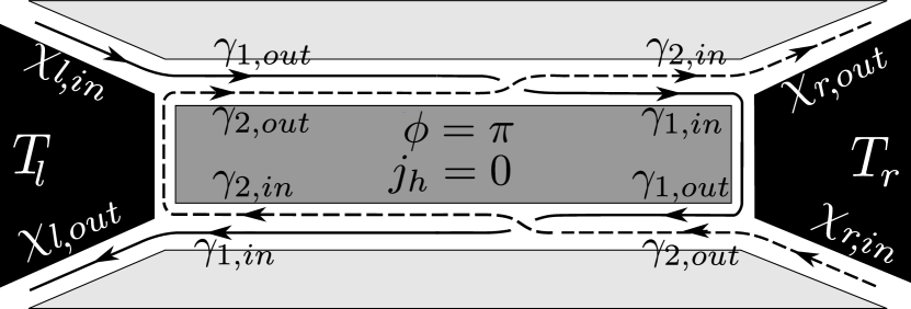
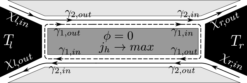
Figure 5: Scattering in the basis of the neutral modes $\chi,\gamma_{1}$ and $\gamma_{2}$ at a zero heat current (upper panel with $\phi=\pi$) and at the maximum of $j_{h}=\frac{\pi^{2}k_{\rm B}^{2}}{12h}(T_{l}^{2}-T_{r}^{2})$ (lower panel with $\phi=0$)

The incoming $\chi_{l,in}$ mode in the left lead converts into $\gamma_{1}$, propagates to the right lead, scatters in the normal region and flows back to the left edge. There is no mixing between $\gamma_{1}$ (solid curve) and $\gamma_{2}$ (dashed curve) and no energy exchange between the two SCs. Hence, the heat current is zero. In the opposite case of the maximal heat current which is equivalent to $\alpha=\alpha_{l}=\alpha_{r}=0$, the mode $\chi_{l,in}$ converts into $\gamma_{2}$ in the left lead and flows away as $\chi_{r,out}$ in the right one.

VII Conclusions

We have analyzed the thermoelectric and heat transport in a long 1D ballistic Josephson junction where the leads are formed by gapless chiral Majorana channels. Such a junction can be realized as a hybrid structure based on a 3D topological insulator surface in the proximity with s-wave superconducting and magnetic films. The interfaces of the gapped sectors support neutral and charged 1D chiral liquids. The normal region is formed by two chiral Dirac liquids spaced by a magnetic material. The chiral contact is formed by four Y-junctions which serve as Dirac-Majorana converters. Our crucial assumption is that the Thouless energy, proportional to the inverse dwell time in the interferometer, is much lower than the superconducting and exchange gaps.

We have obtained the following results. (i) We have generalized the current-phase relation from our previous work  ShapiroShnirmanMirlin to nonidentical Dirac-Majorana contacts and discovered a nonzero Josephson current in the absence of the phase bias, the Aharonov-Bohm phase, and temperature gradient. (ii) We have calculated the thermoelectric current and (iii) the heat current as functions of the magnetic flux and the temperatures of the leads. An important difference of the chiral contact from junctions based on a 2D TI, quantum Hall bar or a spin-orbit coupled nanowire is the absence of a quasiparticle gap in the leads due to the gapless Majorana modes. This results in the absence of the temperature threshold in the current-flux relations. We observe a non-sinusoidal $2\Phi_{0}$-periodic dependence of the thermoelectric and heat currents on the magnetic flux. The maximum oscillation amplitude of the thermoelectric current is proportional to $eE_{Th}/\hbar$ and scales as one over the device size. The maximal amplitude is achieved at a low temperature in one of the superconductors and a high temperature in the other one, i.e. at $T_{l}\gg E_{Th}\gg T_{r}$ or $T_{r}\gg E_{Th}\gg T_{l}$. The heat current oscillates between zero and a value that corresponds to one half of the heat conductance quantum.

VIII Acknowledgments

This research was financially supported by the DFG-RSF grant (No. 16-42-01035 (Russian node) and No. SH 81/4-1, MI 658/9-1 (German node)). DEF’s research was supported in part by the National Science Foundation under Grants No. DMR-1607451 and PHY-1125915.

References

- (1) A. Yu. Kitaev, Phys. Usp. 44 (suppl.), 131 (2001).
- (2) C. Nayak, S. H. Simon, A. Stern, M. Freedman, and S. Das Sarma, Rev. Mod. Phys. , 1083 (2008).
- (3) For a review of proposed states, see G. Yang and D. E. Feldman, Phys. Rev. B 88, 085317 (2013).
- (4) P. T. Zucker and D. E. Feldman, Phys. Rev. Lett. 117, 096802 (2016).
- (5) D. E. Feldman and F. Li, Phys. Rev. B 78, 161304(R) (2008).
- (6) A. Seidel and K. Yang, Phys. Rev. B 80, 241309(R) (2009).
- (7) C. Wang and D. E. Feldman, Phys. Rev. B 81, 035318 (2010).
- (8) L. Fu and C. L. Kane, Phys. Rev. Lett. 100, 096407 (2008).
- (9) L. Fu and C. L. Kane, Phys. Rev. Lett. 102, 216403 (2009).
- (10) X.-L. Qi and S.-C. Zhang, Rev. Mod. Phys. 83, 1057 (2011).
- (11) J. Alicea, Rep. Prog. Phys. 75, 076501 (2012).
- (12) Q. L. He, L. Pan, A. L. Stern, E. Burks, X. Che, G. Yin, J. Wang, B. Lian, Q. Zhou, E. S. Choi, K. Murata, X. Kou, T. Nie, Q. Shao, Y. Fan, S.-C. Zhang, K. Liu, J. Xia, and K. L. Wang, arXiv:1606.05712 (2016).
- (13) G. C. Ménard, S. Guissart, C. Brun, M. Trif, F. Debontridder, R. T. Leriche, D. Demaille, D. Roditchev, P. Simon, and T. Cren, arXiv:1607.06353 (2016).
- (14) A. R. Akhmerov, J. Nilsson, and C.W. J. Beenakker, Phys. Rev. Lett. 102, 216404 (2009).
- (15) K. T. Law, P. A. Lee, and T. K. Ng, Phys. Rev. Lett. 103, 237001 (2009).
- (16) J. Li, G. Fleury, and M. Büttiker, Phys. Rev. B 85, 125440 (2012).
- (17) G. Strübi, W. Belzig, M. S. Choi, and C. Bruder, Phys. Rev. Lett. 107, 136403 (2011).
- (18) D. S. Shapiro, A. Shnirman, and A. D. Mirlin, Phys. Rev. B 93, 155411 (2016).
- (19) C.-Y. Hou, K. Shtengel, and G. Refael, Phys. Rev. B 88, 075304 (2013).
- (20) J. P. Ramos-Andrade, O. Ávalos-Ovando, P. A. Orellana, and S. E. Ulloa, Phys. Rev. B 94, 155436 (2016).
- (21) J. A. M. van Ostaay, A. R. Akhmerov, and C. W. J. Beenakker, Phys. Rev. B 83, 195441 (2011).
- (22) A. Yu. Zyuzin, Phys. Rev. B 50, 323 (1994).
- (23) F. Amet, C. T. Ke, I. V. Borzenets, J. Wang, K. Watanabe, T. Taniguchi, R. S. Deacon, M. Yamamoto, Y. Bomze, S. Tarucha, and G. Finkelstein, Science 352, 966 (2016).
- (24) S.-P. Lee, K. Michaeli, J. Alicea, and A. Yacoby, Phys. Rev. Lett. 113, 197001 (2014).
- (25) G. Tkachov, P. Burset, B. Trauzettel, and E.M. Hankiewicz, Phys. Rev. B 92, 045408 (2015).
- (26) B. Baxevanis, V. P. Ostroukh, and C. W. J. Beenakker, Phys. Rev. B 91, 041409(R) (2015).
- (27) S. V. Mironov, A. S. Mel’nikov, and A. I. Buzdin Phys. Rev. Lett. 114, 227001 (2015).
- (28) B. Sothmann and E. M. Hankiewicz, Phys. Rev. B 94, 081407 (2016).
- (29) B. Sothmann, F. Giazotto, and E. M. Hankiewicz, arXiv:1610.06099 (2016).
- (30) N. V. Gnezdilov, B. van Heck, M. Diez, Jimmy A. Hutasoit, and C. W. J. Beenakker, Phys. Rev. B 92, 121406(R) (2015).
- (31) S. Jezouin, F. D. Parmentier, A. Anthore, U. Gennser, A. Cavanna, Y. Jin, and F. Pierre, Science 342, 601 (2013).
- (32) M. Banerjee, M. Heiblum, A. Rosenblatt, Y. Oreg, D. E. Feldman, A. Stern, and V. Umansky, Nature (London) 545, 75 (2017).
- (33) L. Jiang, D. Pekker, J. Alicea, G. Refael, Y. Oreg, and F. von Oppen, Phys. Rev. Lett. 107, 236401 (2011).
- (34) L. Fu and C. L. Kane, Phys. Rev. B 79, 161408 (2009).
- (35) D. M. Badiane, M. Houzet, and J. S. Meyer, Phys. Rev. Lett. 107, 177002 (2011).
- (36) C. W. J. Beenakker, D. I. Pikulin, T. Hyart, H. Schomerus, and J. P. Dahlhaus, Phys. Rev. Lett. 110,. 017003 (2013).
- (37) P. A. Ioselevich and M.V. Feigel’man, Phys. Rev. Lett. 106, 077003 (2011).
- (38) V. Mourik, K. Zuo, S. M. Frolov, S. R. Plissard, E. P. A. M. Bakkers, and L. P. Kouwenhoven, Science 336, 1003 (2012).
- (39) Ya. M. Blanter and M. Büttiker, Phys. Rep. 336, 1 (2000).
- (40) A. Buzdin, Phys. Rev. Lett. 101, 107005 (2008).
- (41) E. Goldobin, D. Koelle, R. Kleiner, and R. G. Mints, Phys. Rev. Lett. 107, 227001 (2011).
- (42) H. Sickinger, A. Lipman, M.Weides, R. G.Mints, H. Kohlstedt, D. Koelle, R. Kleiner, and E. Goldobin, Phys. Rev. Lett. 109, 107002 (2012).
- (43) C. Winkelholz, Rosario Fazio, F. W. J. Hekking, and G. Schön, Phys. Rev. Lett. 77, 3200 (1996).
- (44) D. L. Maslov, M. Stone, P. M. Goldbart, D. Loss, Phys. Rev. B 53, 1548 (1996).
- (45) R. Fazio, F. W. J. Hekking, and A. A. Odintsov, Phys. Rev. B 53, 6653 (1996).
- (46) P. Dubos, H. Courtois, B. Pannetier, F. K. Wilhelm, A. D. Zaikin, and G. Schön, Phys. Rev. B 63, 064502 (2001).
- (47) A. Levchenko, A. Kamenev, and L. Glazman, Phys. Rev. B 74, 212509 (2006).