Mean-field limits for large-scale random-access networks

Abstract

We establish mean-field limits for large-scale random-access networks with buffer dynamics and arbitrary interference graphs. While saturated-buffer scenarios have been widely investigated and yield useful throughput estimates for persistent sessions, they fail to capture the fluctuations in buffer contents over time, and provide no insight in the delay performance of flows with intermittent packet arrivals. Motivated by that issue, we explore in the present paper random-access networks with buffer dynamics, where flows with empty buffers refrain from competition for the medium. The occurrence of empty buffers thus results in a complex dynamic interaction between activity states and buffer contents, which severely complicates the performance analysis. Hence we focus on a many-sources regime where the total number of nodes grows large, which not only offers mathematical tractability but is also highly relevant with the densification of wireless networks as the Internet of Things emerges. We exploit time scale separation properties to prove that the properly scaled buffer occupancy process converges to the solution of a deterministic initial-value problem, and establish the existence and uniqueness of the associated fixed point. This approach simplifies the performance analysis of networks with huge numbers of nodes to a low-dimensional fixed-point calculation. For the case of a complete interference graph, we demonstrate asymptotic stability, provide a simple closed-form expression for the fixed point, and prove interchange of the mean-field and steady-state limits. This yields asymptotically exact approximations for key performance metrics, in particular the stationary buffer content and packet delay distributions.

This work was done while F.Cecchi was at Eindhoven University of Technology.

1 Introduction

1.1 Background and related work

Wireless networks are already large and complex today, and being at the heart of the so-called Internet of Things (IoT) [1], are expected to grow even denser in the future [20]. Obviously, when the number of nodes is large, in the hundreds or even thousands of nodes, a dedicated medium or channel cannot be assigned to each node, and nodes have to share the medium. Medium access control (MAC) mechanisms are therefore crucial to resolve the contention among the various nodes. However, in large networks, a centralized control mechanism is hard to implement and to maintain since it would require constant status updates generating prohibitive communication overhead. For this reason the design of efficient distributed (local) MAC protocols has attracted a lot of attention.

A very popular distributed MAC mechanism is the CSMA (Carrier-Sense Multiple-Access) protocol, which is currently at the core of the IEEE 802.11 and 802.15.4 standards. Its popularity is mostly due to its simplicity and efficiency. The key feature of the CSMA protocol is that each node waits for a random back-off period before initiating a transmission. Interference is avoided since the back-off countdown is interrupted whenever potential interference is sensed, and only resumed once the medium is sensed idle again. This protocol, whilst extremely easy to understand on a local level, generates complex and interesting macroscopic network dynamics.

In the performance analysis of CSMA networks, a common assumption is the existence of an underlying graph that represents interference between the various nodes in the network. An edge between two nodes means that destructive interference is caused by simultaneous transmission. Both empirical and theoretical support for the notion of an interference graph is provided in [24, 40].

When the nodes always have packets to transmit, the network is said to be saturated and the macroscopic activity behavior is amenable to analysis under the assumption of an interference graph. In particular, the activity process has an elegant product-form stationary distribution [6, 29, 34]. The computation of the stationary distribution of the activity process reduces to the identification of all the subsets of nodes which may transmit simultaneously, namely the independent sets of the interference graph.

Real-life scenarios however involve unsaturated networks. Packets arrive at the various nodes according to exogenous processes, and buffers may drain from time to time as packets are transmitted. In particular, in IoT applications, sources are likely to generate packets only sporadically, with fairly tight delay constraints, and often have empty buffers. Since empty nodes temporarily refrain from the medium competition, the activity process is strictly intertwined with the buffer content process. In this situation, the product-form solution no longer holds [11, 34] and an exact stationary analysis does not seem tractable.

The analysis of unsaturated CSMA networks simplifies if certain symmetry conditions amongst the various nodes hold. An important instance is when there is a substantial number of nodes with similar traffic and placement in the network, so that the operation of one is equivalent to that of many others. More generally, nodes can be divided into classes with the symmetry conditions now applying to nodes of the same class. The asymptotic regime where the number of such nodes in each class grows to infinity, is commonly referred to as a mean-field regime. Mean-field theory originated in physics, where it is still widely used in analyzing models involving a large number of interacting particles. The aggregated effect of all the other nodes on any tagged node is approximated by a single averaged effect (the mean-field), thus reducing a many-body problem to a more tractable one-body problem. In the context of random-access networks, a mean-field regime not only provides analytical tractability, but is also highly relevant in the context of the envisioned massive numbers of IoT devices.

A thorough survey of mean-field analysis of random-access protocols is presented in [18]. The work of Bianchi [3] is a landmark paper which assumed nodes to behave independently one from the other in the regime where many of them are present so as to derive tractable formulae for the key performance measures of the system. The papers surveyed in [18] mostly use mean-field theory to provide either evidence or objection for the assumption of Bianchi. Among these papers, it is worth mentioning [13], where the authors investigated the existence of a global attractor for the mean-field system and provided sufficient conditions for its existence, deducing the validity of Bianchi’s assumption. Further papers which deserve to be mentioned are [7, 32], where the authors exploited mean-field theory so as to obtain approximations for key performance measures of large systems. In particular, [7] focuses on the characterization of the stability region, while [32] examines the throughput performance of the system. None of the above-mentioned papers considered scenarios with unsaturated buffers, with the exception of [7], which however dealt with systems evolving in discrete time and did not consider performance metrics like packet delays.

1.2 Key contributions and paper organization

In the present paper we examine the buffer dynamics in large-scale unsaturated random-access networks. Specifically, we analyze the buffer occupancy processes in a mean-field regime where the number of nodes grows large.

We provide a detailed model description and introduce some useful notation and preliminaries in Section 2. An overview of the main results of the paper is presented in Section 3. In Section 4 we prove for general interference graphs that a suitably scaled version of the buffer occupancy processes converges in the mean-field limit to a tractable deterministic initial-value problem. We also establish necessary and sufficient conditions for the existence and uniqueness of a fixed point of the initial-value problem, and provide a characterization of the fixed point as the solution of a low-dimensional equation. In Section 5 we focus on scenarios with a complete interference graph, and demonstrate global asymptotic stability of the initial-value problem, i.e., convergence to the unique fixed point from any initial state with finite mass. We then proceed to show positive recurrence of the pre-limit process and tightness of the sequence of stationary distributions, and combine these properties to prove interchange of the mean-field and steady-state limits. The interchange of limits is leveraged to establish that the stationary buffer content distributions at the various nodes converge to geometric distributions, while the stationary distributions of the scaled waiting time and sojourn time converge to exponential distributions. The parameters of these limiting distributions are directly expressed in terms of the fixed point of the initial-value problem. These results provide asymptotically exact approximations for the stationary waiting-time and sojourn time distributions. In Section 6 we present some simulation experiments to illustrate the analytical results. Finally, in Section 7 we make a few concluding remarks and offer several suggestions for further research.

2 Model description

We consider a network of $N$ nodes sharing a wireless medium according to a random-access protocol. The various nodes are grouped into a set of classes/clusters $\mathcal{C}=\{1,\dots,C\}$ such that nodes in the same class have the same statistical characteristics. Denote by $N^{(N)}_{c}$ the number of class-$c$ nodes, where $\sum_{c\in\mathcal{C}}N^{(N)}_{c}=N$ and $p_{c,N}=N^{(N)}_{c}/N$.

Interference graph. Given a class-wise interference graph $G=(\mathcal{C},\mathcal{E})$, two nodes interfere when they belong either to the same class or to two neighboring classes in $G$. A feasible class activity state can thus be represented by a vector $\omega\in\{0,1\}^{C}$, with $\omega_{c}=1$ if a class-$c$ node is transmitting in state $\omega$ and $\omega_{c}=0$ otherwise, and $\omega_{c}\omega_{d}=0$ if $(c,d)\in\mathcal{E}$. Let $\Omega$ be the set of all feasible class activity states, which are in one-to-one correspondence with the independent sets of the graph $G$. For every class $c$, we define the following subsets of $\Omega$:

$$\Omega_{-c}\>\dot{=}\>\{\omega\in\Omega:\omega_{c}=0,\omega_{d}=0\>\forall\>d\text{ s.t. }(c,d)\in\mathcal{E}\},$$

$$\Omega_{+c}\>\dot{=}\>\{\omega\in\Omega:\omega_{c}=1\}.$$

This means that $\omega\in\Omega_{-c}$ if and only if in the class activity state $\omega$ none of the nodes belonging to class $c$ or to a class interfering with class $c$ are active, while $\omega\in\Omega_{+c}$ if and only if a class-$c$ node is active. We define the class-capacity region of the network as $\Gamma\doteq\text{Conv}(\Omega)$, i.e.,

$$\Gamma=\{\boldsymbol{\gamma}\in\mathbb{R}_{+}^{C}:\exists\>\boldsymbol{a}=(a_{\omega})_{\omega\in\Omega}\>\text{ s.t. }\>a_{\omega}\geq 0,\sum_{\omega\in\Omega}a_{\omega}\leq 1,\sum_{\omega\in\Omega}a_{\omega}\omega=\boldsymbol{\gamma}\}.$$

As an illustration, Figure 1 shows a square interference graph $G$ with $C=4$ classes of nodes numbered in a clockwise fashion. The activity states are

$$\Omega=\big{\{} (0,0,0,0),(1,0,0,0),(0,1,0,0),(0,0,1,0),$$

$$(0,0,0,1),(1,0,1,0),(0,1,0,1)\big{\}},$$

and the class-capacity region is given by

$$\Gamma=\{\boldsymbol{\gamma}\in\mathbb{R}_{+}^{4}:\max\{\gamma_{1},\gamma_{3}\}+\max\{\gamma_{2},\gamma_{4}\}\leq 1\}.$$

Taking $c=1$ the sets $\Omega_{-c},\Omega_{+c}\subset\Omega$ are

$$\Omega_{-1} = \left\{(0,0,0,0),(0,0,1,0)\right\}$$

$$\Omega_{+1} = \left\{(1,0,0,0),(1,0,1,0)\right\}.$$

Figure 1: A square interference graph with $C=4$.

Network dynamics. Nodes within the same class share the same statistical features. Packets arrive at the various class-$c$ nodes as independent Poisson processes of rate $\lambda_{c}^{(N)}\>\dot{=}\>\lambda_{c}/N^{(N)}_{c}$. Once a class-$c$ node obtains access to the medium, it transmits one packet, which takes an exponentially distributed time with parameter $\mu_{c}^{(N)}\>\dot{=}\>\mu_{c}$. In between two consecutive transmissions a class-$c$ node must back-off for an exponentially distributed time period with parameter $\nu_{c}^{(N)}\>\dot{=}\>\nu_{c}/N^{(N)}_{c}$. Note that a node refrains from the back-off competition whenever its buffer is empty. Also, the back-off period of a class-$c$ node is suspended (frozen) when the medium is occupied by an interfering node, i.e., the class activity state does not belong to $\Omega_{-c}$.

Define the queue length process $\boldsymbol{Q}^{(N)}(t)=(Q_{c,k}^{(N)}(t))_{c\in\mathcal{C},k=1,\ldots,N_{c}}$, where $Q_{c,k}^{(N)}(t)$ represents the number of packets in the buffer of the $k$-th node belonging to class $c$ at time $t$ excluding any possible packet in transmission, and define by $\boldsymbol{Y}^{(N)}(t)$ the class activity process on the state space $\Omega$. Observe that $\big{(}\boldsymbol{Q}^{(N)}(t),\boldsymbol{Y}^{(N)}(t)\big{)}$ evolves as a Markov process.

A population process description. To ease the notation we write $N_{c}=N^{(N)}_{c}$ whenever possible. Due to the class symmetry, the nodes within a class are statistically indistinguishable, and the system state may be described in terms of the numbers of nodes belonging to the same class and with the same number of packets in the buffer. In particular, define the population process $\tilde{\boldsymbol{X}}^{(N)}(t)=(\tilde{X}_{c,n}^{(N)}(t))_{c\in\mathcal{C},n\in\mathbb{N}_{0}}$, where

$$\tilde{X}_{c,n}^{(N)}(t)=\frac{1}{N_{c}}\sum_{k=1}^{N_{c}}\mathbbm{1}\{Q_{c,k}^{(N)}(t)=n\}.$$

The process $\big{(}\tilde{\boldsymbol{X}}^{(N)}(t),\boldsymbol{Y}^{(N)}(t)\big{)}$ is itself Markovian with state space $E\times\Omega$, where

$$E\>\dot{=}\>\chi^{C},\qquad\chi\>\dot{=}\>\{\boldsymbol{x}=(x_{n})_{n\in\mathbb{N}_{0}}:\sum_{n\in\mathbb{N}_{0}}x_{n}\leq 1,\>x_{n}\geq 0,\>\forall n\in\mathbb{N}_{0}\}.$$ (1)

Observe that the population process lies in $E^{1}\subseteq E$ where

$$E^{1}\>\dot{=}\>\{\boldsymbol{x}\in E\>:\sum_{n=0}^{\infty}x_{c,n}=1,\>\forall c\in\mathcal{C}\}.$$ (2)

The possible transitions for the process $\big{(}\tilde{\boldsymbol{X}}^{(N)}(t),\boldsymbol{Y}^{(N)}(t)\big{)}$ may be described as follows:

•  A packet arrives at a class-$c$ node having $n$ packets in its buffer: this happens at rate $\lambda_{c}^{(N)}$ times the number of class-$c$ nodes in state $n$, i.e., $\lambda_{c}^{(N)}N_{c}\tilde{X}^{(N)}_{c,n}=\lambda_{c}\tilde{X}^{(N)}_{c,n}$, and generates the transition

$$\begin{cases}\tilde{X}_{c,n}^{(N)}\rightarrow\tilde{X}_{c,n}^{(N)}-\frac{1}{N_{c}}\\ \tilde{X}_{c,n+1}^{(N)}\rightarrow\tilde{X}_{c,n+1}^{(N)}+\frac{1}{N_{c}},\end{cases}$$

i.e.,

$$(\tilde{\boldsymbol{X}}^{(N)},\boldsymbol{Y}^{(N)})\rightarrow(\tilde{\boldsymbol{X}}^{(N)}+\frac{1}{N_{c}}\boldsymbol{e}^{c,n+1}_{c,n},\boldsymbol{Y}^{(N)}),$$

where $\boldsymbol{e}^{c_{1},n_{1}}_{c_{2},n_{2}}=\boldsymbol{e}_{c_{1},n_{1}}-\boldsymbol{e}_{c_{2},n_{2}}$ and $\boldsymbol{e}_{c,n}\in\chi^{C}$ has all $0$ entries except a $1$ in position $(c,n)$.

•  A transmission is completed by a class-$c$ node: this happens at rate $\mu_{c}^{(N)}=\mu_{c}$ and only if a class-$c$ node is transmitting, i.e., $\boldsymbol{Y}^{(N)}\in\Omega_{+c}$. The transition generated is the following

$$(\tilde{\boldsymbol{X}}^{(N)},\boldsymbol{Y}^{(N)})\rightarrow(\tilde{\boldsymbol{X}}^{(N)},\boldsymbol{Y}^{(N)}-\boldsymbol{e}_{c}),$$

where $\boldsymbol{e}_{c}\in\{0,1\}^{C}$ has all $0$ entries except a $1$ in position $c$.

•  A back-off is completed by a class-$c$ node having $n>0$ packets in its buffer: this happens only if the class activity state allows class-$c$ nodes to back-off, i.e., $\boldsymbol{Y}^{(N)}\in\Omega_{-c}$, and at rate $\nu_{c}^{(N)}$ times the number of class-$c$ nodes in state $n$, i.e., $\nu_{c}^{(N)}N_{c}\tilde{X}^{(N)}_{c,n}=\nu_{c}\tilde{X}^{(N)}_{c,n}$, and generates the transition

$$\begin{cases}\boldsymbol{Y}^{(N)}\rightarrow\boldsymbol{Y}^{(N)}+\boldsymbol{e}_{c}\\ \tilde{X}_{c,n}^{(N)}\rightarrow\tilde{X}_{c,n}^{(N)}-\frac{1}{N_{c}}\\ \tilde{X}_{c,n-1}^{(N)}\rightarrow\tilde{X}_{c,n-1}^{(N)}+\frac{1}{N_{c}},\end{cases}$$

i.e.,

$$(\tilde{\boldsymbol{X}}^{(N)},\boldsymbol{Y}^{(N)})\rightarrow(\tilde{\boldsymbol{X}}^{(N)}+\frac{1}{N_{c}}\boldsymbol{e}^{c,n-1}_{c,n},\boldsymbol{Y}^{(N)}+\boldsymbol{e}_{c}).$$

Preliminary results for saturated scenario. As mentioned earlier, we focus on an unsaturated network where nodes with empty buffers refrain from competition for the medium. For later purposes, it is convenient to also consider a related saturated network where each class behaves as a single node always competing for the medium, and backing-off at rate $\eta_{c}\nu_{c}$, where $\boldsymbol{\eta}=(\eta_{c})_{c\in\mathcal{C}}\in\mathbb{R}_{+}^{C}$. The transmission times of the node associated with class $c$ are exponentially distributed with parameter $\mu_{c}$.

For compactness, denote $\sigma_{c}=\nu_{c}/\mu_{c}$, and for any $\boldsymbol{\eta}\in\mathbb{R}_{+}^{C}$,

$$Z(\omega;\boldsymbol{\eta})\>\dot{=}\>\prod_{c\in\mathcal{C}}(\eta_{c}\sigma_{c})^{\omega_{c}},\qquad\omega\in\Omega,$$

and

$$Z(\boldsymbol{\eta})\>\dot{=}\>\sum_{\omega\in\Omega}Z(\omega;\boldsymbol{\eta}).$$

The activity process in this fictitious saturated network has a product-form stationary distribution [6, 34, 36]

$$\pi(\omega;\boldsymbol{\eta})=\frac{Z(\omega;\boldsymbol{\eta})}{Z(\boldsymbol{\eta})},\qquad\omega\in\Omega.$$ (3)

Define now the throughput function $\boldsymbol{\theta}:\mathbb{R}_{+}^{C}\rightarrow\Gamma$, where

$$\theta_{c}(\boldsymbol{\eta})\>\dot{=}\>\sum_{\omega\in\Omega}\omega_{c}\pi(\omega;\boldsymbol{\eta})=\sum_{\omega\in\Omega_{+c}}\pi(\omega;\boldsymbol{\eta})=\pi(\Omega_{+c};\boldsymbol{\eta})$$ (4)

represents the fraction of time that the node associated with class $c$ is active in the saturated network in stationarity.

As proved in [26, 35], the throughput map $\boldsymbol{\theta}$ is globally invertible, i.e., for any achievable throughput vector $\boldsymbol{\gamma}\in\text{int}(\Gamma)$ there exists a unique vector $\boldsymbol{\eta}(\boldsymbol{\gamma})\in{\mathbb{R}}_{+}^{C}$ such that

$$\boldsymbol{\theta}(\boldsymbol{\eta}(\boldsymbol{\gamma}))=\boldsymbol{\gamma}.$$ (5)

Intuitively, the $c$-th coordinate of $\boldsymbol{\eta}(\boldsymbol{\gamma})$ represents by what factor the back-off rate at node $c$ needs to accelerate/decelerate in order for the target throughput vector $\boldsymbol{\gamma}$ to be achieved in stationarity.

3 Overview of the main results

In this section we provide an overview of the main results of the paper, along with an interpretation and high-level discussion of their ramifications, before presenting the proofs in the subsequent sections.

We first analyze networks with general class-based interference graphs, and define

$$\boldsymbol{X}^{(N)}(t)\doteq\tilde{\boldsymbol{X}}^{(N)}(Nt)$$

as the fluid version of the population process. We consider a sequence of processes $\boldsymbol{X}^{(N)}(t)$ as the number of nodes in the system increases, and establish its weak convergence to $\boldsymbol{x}(t)$, the solution of a tractable deterministic initial-value problem as stated in the next theorem.

Theorem 3.1.

Assume $\boldsymbol{X}^{(N)}(0)\xrightarrow{N\rightarrow\infty}\boldsymbol{x}^{\infty}\in E^{1}$ and $\lim_{N\rightarrow\infty}p_{c,N}=p_{c}>0$ for every $c\in\mathcal{C}$. Then the sequence of processes

$$(\boldsymbol{X}^{(N)}(t))\in D_{E^{1}}[0,\infty)$$

has a continuous limit $\boldsymbol{x}(t)\in C_{E^{1}}[0,\infty)$ which is determined by the unique solution of the initial-value problem

$$\frac{d\boldsymbol{x}(t)}{dt}=H(\boldsymbol{x}(t)),\qquad\boldsymbol{x}(0)=\boldsymbol{x}^{\infty},$$ (6)

where the function $H(\cdot)$ is defined by

$$H(\boldsymbol{x})= \sum_{c\in\mathcal{C}}\frac{1}{p_{c}}\Big{(}\lambda_{c}\sum_{n=0}^{\infty}x_{c,n}\boldsymbol{e}^{c,n+1}_{c,n}+\pi_{\boldsymbol{x}_{0}}(\Omega_{-c})\nu_{c}\sum_{n=1}^{\infty}x_{c,n}\boldsymbol{e}^{c,n-1}_{c,n}\Big{)}$$

with

$$\pi_{\boldsymbol{x}_{0}}(\Omega_{-c})=\sum_{\omega\in\Omega_{-c}}\pi_{\boldsymbol{x}_{0}}(\omega),\qquad\pi_{\boldsymbol{x}_{0}}(\omega)\doteq\pi(\omega;\boldsymbol{e}-\boldsymbol{x}_{0}),$$

$\boldsymbol{x}_{0}=(x_{1,0},\ldots,x_{C,0})$, and $\boldsymbol{e}$ has every component equal to $1$.

The major difficulty in the analysis of unsaturated networks arises from the correlation between the population process $\tilde{\boldsymbol{X}}^{(N)}(t)$ and the activity process $\boldsymbol{Y}^{(N)}(t)$. A key observation in the proof of Theorem 3.1 is that these processes evolve on different time scales, i.e., the population process evolves $N$ times slower than the activity process. Hence, in the mean-field regime, the rapidly changing activity process “converges to an instantaneous measure on the activity states” determined by the current fraction of queues which are empty. This is the reason why the initial-value problem (6) does not explicitly involve the activity process and the evolution of the population process at time $t$ depends only on $\boldsymbol{x}(t)$. Specifically, the fraction of class-$c$ nodes with $n\geq 1$ packets in the buffer “increases” at rate $\lambda_{c}$ and “decreases” at rate $\nu_{c}\pi_{\boldsymbol{x}_{0}}(\Omega_{-c})$, where the measure $\pi_{\boldsymbol{x}_{0}}(\Omega_{-c})$ represents the limiting “instantaneous measure” on the activity states that allows class-$c$ nodes to back-off. The argument is thus based on a stochastic averaging principle which follows the same lines of ideas of [21, 25].

The initial-value problem (6) is certainly easier to analyze than the population process in a network with a finite number of nodes. Theorem 3.2 states that, under certain necessary and sufficient conditions, there exists a unique fixed point $\boldsymbol{x}^{*}$ for the initial-value problem (6), and provides its characterization in terms of the load of the network.

Theorem 3.2.

If $\boldsymbol{\rho}\in\mbox{int}(\Gamma)$ and $\boldsymbol{\xi}=\boldsymbol{\eta}(\boldsymbol{\rho})<\boldsymbol{e}$, where $\boldsymbol{\eta}(\cdot)$ is defined in (5), then $\boldsymbol{x}^{*}\in E^{1}$, with

$$x_{c,n}^{*}=(1-\xi_{c})\xi_{c}^{n},$$ (7)

is the unique fixed point of the initial-value problem (6) in $E^{1}$, i.e., $H(\boldsymbol{x}^{*})=\boldsymbol{0}$.

Specifically, the condition $\boldsymbol{\rho}\in\mbox{int}(\Gamma)$ is necessary for existence and ensures the load $\boldsymbol{\rho}$ of the system is sustainable. On the other hand, the condition $\boldsymbol{\xi}=\boldsymbol{\eta}(\boldsymbol{\rho})<\boldsymbol{e}$ ensures that the desired throughput vector $\boldsymbol{\rho}$ can be achieved by a feasible back-off vector. Although Theorem 3.2 only concerns the scaled population process, combined with Theorem 3.1 it yields that the stationary distribution of the associated class activity process is given by $\pi_{\boldsymbol{x}_{0}^{*}}\in\mathbb{P}(\Omega)$ in the limit. In other words, in the limit the stationary distribution of the class activity process is the same as in a scenario where the aggregate back-off rate of class $c$ is a constant fraction $\xi_{c}$ of the nominal back-off rate $\nu_{c}$. This is consistent with the fact that $\xi_{c}$ is the stationary fraction of class-$c$ nodes that have non-empty buffers and compete for the medium, and $\boldsymbol{\xi}$ will therefore in the sequel be referred to as the vector of activity factors. The equation $\boldsymbol{\xi}=\boldsymbol{\eta}(\boldsymbol{\rho})$ reflects that the activity factors must be such that each class $c$ is active a fraction $\rho_{c}$ of the time.

Figure 2: Diagram for the interchange of limits.

We will use the above convergence properties of the population process to derive asymptotically exact results for the key performance measures of the system. For a rigorous treatment, we focus on the scenario where all the classes mutually interfere, i.e., the interference graph $G=(\mathcal{C},\mathcal{E})$ is complete, in which case

$$\Gamma=\{\boldsymbol{\gamma}\in\mathbb{R}^{C}:\sum_{c\in\mathcal{C}}\gamma_{c}\leq 1\}.$$

In this framework, the nodes of every class are allowed to back-off only when the activity process is in the idle state. We will show that the vector of activity factors $\boldsymbol{\xi}$ in Theorem 3.2 simplifies to

$$\xi_{c}=\frac{\lambda_{c}}{\nu_{c}\big{(}1-\sum_{d\in\mathcal{C}}\frac{\lambda_{d}}{\mu_{d}}\big{)}},$$

so that the condition $\boldsymbol{\xi}=\boldsymbol{\eta}(\boldsymbol{\rho})<\boldsymbol{e}$ can be expressed in explicit form as

$$\max_{c\in\mathcal{C}}\frac{\lambda_{c}}{\nu_{c}}<1-\sum_{d\in\mathcal{C}}\frac{\lambda_{d}}{\mu_{d}},$$ (8)

which forces the right-hand side to be positive, i.e., $\boldsymbol{\rho}\in\mbox{int}(\Gamma)$. When condition (8) applies, Theorem 3.3 holds and asymptotically characterizes the stationary distribution of the population process as the fixed point of the initial-value problem (6).

Theorem 3.3.

The sequence of stationary random variables $(\boldsymbol{X}_{*}^{(N)})_{N\geq 1}$ weakly converges to ${\boldsymbol{x}^{*}}\in E^{1}$, i.e.,

$$\boldsymbol{X}_{*}^{(N)}\>\>\xRightarrow{N\rightarrow\infty}\>\>\boldsymbol{x}^{*}.$$ (9)

In order to prove Theorem 3.3, we show that the interchange of limits displayed in Figure 2 holds. Specifically, the methodology developed reduces the derivation of the stationary distribution of an intractable $N$-dimensional Markov process to the computation of the fixed point of a low-dimensional fixed-point equation.

Theorem 3.3 is exploited so as to obtain approximations for the performance measures of the system. In particular, denote by $Q_{c}^{(N)}$ the stationary queue length at a class-$c$ node, and by $W_{c}^{(N)}$ and $S_{c}^{(N)}$ the stationary waiting time and sojourn time of a packet at a class-$c$ node, respectively. Assume condition (8) holds.

Theorem 3.4.

For every class $c$,

$$Q_{c}^{(N)}\Rightarrow\bar{Q}_{c},\qquad\frac{\lambda_{c}}{N_{c}}S_{c}^{(N)}\Rightarrow\bar{S}_{c},\qquad\frac{\lambda_{c}}{N_{c}}W_{c}^{(N)}\Rightarrow\bar{W}_{c},$$

where

$$\bar{Q}_{c}\sim\text{Geo}(\xi_{c}),\qquad\bar{W}_{c}\sim\bar{S}_{c}\sim\text{Exp}\big{(}\frac{1-\xi_{c}}{\xi_{c}}\big{)},\qquad c\in\mathcal{C}.$$

Theorem 3.5.

For every class $c$,

$$\mathbb{E}[Q_{c}^{(N)}]\rightarrow\mathbb{E}[\bar{Q}_{c}],\qquad\frac{\lambda_{c}}{N_{c}}\mathbb{E}[W_{c}^{(N)}]\rightarrow\mathbb{E}[\bar{W}_{c}],\qquad\frac{\lambda_{c}}{N_{c}}\mathbb{E}[S_{c}^{(N)}]\rightarrow\mathbb{E}[\bar{S}_{c}].$$

These theorems show that, given any node in the system, its stationary queue length converges in distribution and expectation to a geometric random variable, while the scaled waiting time and sojourn time of a packet in its buffer converge to exponentially distributed random variables. These limits can be used as approximations for the performance of finite-node systems, which are provably exact as the number of nodes in the network grows large, and remain very accurate when the size of the network is moderate [10, Section 4.6].

4 Mean-field limit in a general framework

In this section we present the proofs of Theorems 3.1 and 3.2 as stated in Section 3.

4.1 Derivation of the mean-field limit

Theorem 3.1 describes the weak limit of the sequence of processes $\{\boldsymbol{X}^{(N)}(t)\}_{N\in\mathbb{N}}$, which is known as the mean-field limit of the population process. In order to prove Theorem 3.1, we need to go through various steps which we briefly outline here.

1. In Section 4.1.1, a Poisson representation for the prelimit process

   $$\big{(}\tilde{\boldsymbol{X}}^{(N)}(t),\boldsymbol{Y}^{(N)}(t)\big{)}$$

   is provided. This representation allows us to easily derive the dynamics of the process on a fluid time scale.

2. In Section 4.1.2 a detour is needed in order to ensure the existence of the limiting process. Specifically, the class activity process $\boldsymbol{Y}^{(N)}$ is replaced by a cumulative time process $\boldsymbol{\alpha}^{(N)}$, so that the evolution of the model on fluid time scale can be equivalently described via the process

   $$\big{(}\boldsymbol{X}^{(N)}(t),\boldsymbol{\alpha}^{(N)}(t)\big{)}.$$ (10)

   Finally, the sequence of processes (10) is shown to weakly converge as $N\rightarrow\infty$ to a limiting process

   $$\big{(}\boldsymbol{x}(t),\boldsymbol{\alpha}(t)\big{)}.$$ (11)

3. In Section 4.1.3 we characterize the limiting process (11).

4. As a last step, in Section 4.1.4, we describe how the limiting process $\boldsymbol{\alpha}(t)$ at time $t$ is uniquely determined by the value $\boldsymbol{x}(t)$. Hence a self-contained deterministic initial-value problem governing the behavior of $\boldsymbol{x}(t)$ is obtained.

In preparation for the analysis, we briefly recall a few useful properties of the topological space where the population process evolves. The sample paths of $\boldsymbol{X}^{(N)}(t)$ lie in $D_{E}[0,\infty)$, i.e., the set of the cadlag functions from $[0,\infty)$ in $E=\chi^{C}$, where the space $E$ is defined in (1). Define on $E$ the metric $\rho(\cdot,\cdot)$ such that

$$\rho\big{(}(\boldsymbol{x}^{(1)}_{c})_{c\in\mathcal{C}},(\boldsymbol{x}^{(2)}_{c})_{c\in\mathcal{C}}\big{)}=\sum_{c\in\mathcal{C}}\rho_{1}(\boldsymbol{x}^{(1)}_{c},\boldsymbol{x}^{(2)}_{c}),$$

where $\boldsymbol{x}_{c}=(x_{c,n})_{n\in\mathbb{N}_{0}}\in\chi$ and $\rho_{1}$ is a metric on $\mathbb{R}^{\infty}$, i.e.,

$$\rho_{1}(\boldsymbol{x}^{(1)},\boldsymbol{x}^{(2)})=\sum_{n\in\mathbb{N}_{0}}2^{-n}\frac{|x_{n}^{(1)}-x_{n}^{(2)}|}{1+|x_{n}^{(1)}-x_{n}^{(2)}|}.$$

Note that $(\mathbb{R}^{\infty},\rho_{1})$ is separable and complete, and $\chi$ is compact in $(\mathbb{R}^{\infty},\rho_{1})$ as each coordinate lies in $[0,1]$, see [4, page 219]. From [5, Section M6, pages 240-241], the following lemma is therefore obtained.

Lemma 4.1.

The subset $E=\chi^{C}$ is complete, separable, and compact under the product topology induced by the metric $\rho$ in the space $\prod_{c\in\mathcal{C}}\mathbb{R}^{\infty}$.

In the subsequent analysis we will work with $D_{E}[0,\infty)$ using the metric $d$, an exponentially weighted version of the Skorohod metric, see [19, page 117]. Under this metric $D_{E}[0,\infty)$ is complete and separable as $(E,\rho)$ is itself complete and separable, see [19, Theorem 5.6, page 121].

4.1.1 Unit Poisson process representation

In this subsection we describe the fluid-time marginals of the prelimit Markov population process $\big{(}\tilde{\boldsymbol{X}}^{(N)}(t),\boldsymbol{Y}^{(N)}(t)\big{)}$ in terms of infinite sequences of unit Poisson processes. For each $c\in\mathcal{C}$, and then for each $n\in{\mathbb{N}}_{0}$, the random quantity ${\mathcal{N}}_{\text{A},c,n}(t)$ determines the class-$c$ arrivals to queues with $n$ packets in the buffer during the time interval $[0,t)$. We similarly define ${\mathcal{N}}_{\text{B},c,n}(t)$ for each $c\in\mathcal{C}$, $n\in{\mathbb{N}}$, to determine the back-offs and finally ${\mathcal{N}}_{\text{T},c}(t)$ determines the process of transmissions for each $c\in\mathcal{C}$. These processes are supposed mutually independent and defined on a common probability space $\left(\Omega_{F},\mathcal{F}^{F},\mathbb{P}\right)$. We also define the centered versions of these processes to be $\tilde{\mathcal{N}}_{\text{A},c,n}(s)={\mathcal{N}}_{\text{A},c,n}(s)-s$ for each $c\in\mathcal{C}$, $n\in{\mathbb{N}}_{0}$, with corresponding definitions for the back-offs and the transmissions. These are martingales with respect to their natural filtrations.

To obtain the Poisson process representation, we first fix the initial conditions, which are deterministic. Realizations of the above unit Poisson processes are then drawn and the (unscaled) population random variables $\tilde{\boldsymbol{X}}$, $\boldsymbol{Y}$ are obtained as solutions to the following equations, where fluid time is $t$. That is,

$$\tilde{\boldsymbol{X}}^{(N)}(t)=\> \tilde{\boldsymbol{X}}^{(N)}(0)+\sum_{c\in\mathcal{C}}\sum_{n=0}^{\infty}\frac{\boldsymbol{e}^{c,n+1}_{c,n}}{N_{c}^{(N)}}\tilde{A}_{c,n}(t)+\sum_{c\in\mathcal{C}}\sum_{n=1}^{\infty}\frac{\boldsymbol{e}^{c,n-1}_{c,n}}{N_{c}^{(N)}}\tilde{D}_{c,n}(t)$$

$$\boldsymbol{Y}^{(N)}(t)=\> \boldsymbol{Y}^{(N)}(0)-\sum_{c\in\mathcal{C}}\boldsymbol{e}_{c}\tilde{V}_{c}(t)+\sum_{c\in\mathcal{C}}\sum_{n=1}^{\infty}\boldsymbol{e}_{c}\tilde{D}_{c,n}(t),$$

where

$$\tilde{A}_{c,n}(t) ={\mathcal{N}}_{\text{A},c,n}\Bigl{(}\lambda^{(N)}_{c}\int_{0}^{t}N_{c}^{(N)}\tilde{X}_{c,n}^{(N)}(s)ds\Bigr{)},$$

$$\tilde{D}_{c,n}(t) =\int_{0}^{t}\mathbbm{1}\{\boldsymbol{Y}^{(N)}(s^{-})\in\Omega_{-c}\}d{\mathcal{N}}_{\text{B},c,n}\Bigl{(}\nu_{c}^{(N)}\int_{0}^{s}N^{(N)}_{c}\tilde{X}^{(N)}_{c,n}(u)du\Bigr{)},$$

$$\tilde{V}_{c}(t) =\int_{0}^{t}\mathbbm{1}\{\boldsymbol{Y}^{(N)}(s^{-})\in\Omega_{+c}\}d{\mathcal{N}}_{\text{T},c}\Bigl{(}\mu_{c}^{(N)}\int_{0}^{s}du\Bigr{)}.$$

As observed in the discussion in [28], the solutions to these equations can be obtained by fixing the sample paths of the Poisson processes $\mathcal{N}_{A,c,n}$, $\mathcal{N}_{B,c,n}$, $\mathcal{N}_{T,c}$ above. It can then be seen from the above that, when $\tilde{\boldsymbol{X}}^{(N)}(0)\in E^{1}$, then the sample paths of the process $(\tilde{\boldsymbol{X}}^{(N)}(t),\boldsymbol{Y}^{(N)}(t))$ lie in $D_{E^{1}\times\Omega}$.

We now rewrite these equations in a more compact form, working componentwise. When possible, the $N$ superscript has been omitted for conciseness.

$$X_{c,n}(t) =X_{c,n}(0)+A_{c,n-1}(t)-A_{c,n}(t)+D_{c,n+1}(t)-D_{c,n}(t),$$ (12)

$$Y_{c}(Nt) =Y_{c}(0)+N_{c}\sum_{n=1}^{\infty}D_{c,n}(t)-V_{c}(t),$$ (13)

where

$$A_{c,n}(t) =\frac{1}{N_{c}}{\mathcal{N}}_{\text{A},c,n}\Bigl{(}N\lambda_{c}\int_{0}^{t}X_{c,n}(s)ds\Bigr{)},$$ (14)

$$D_{c,n}(t) =\frac{1}{N_{c}}\int_{0}^{t}\mathbbm{1}\{\boldsymbol{Y}(Ns^{-})\in\Omega_{-c}\}d{\mathcal{N}}_{B,c,n}\Bigl{(}N\nu_{c}\int_{0}^{s}X_{c,n}(u)du\Bigr{)},$$ (15)

$$V_{c}(t) =\int_{0}^{t}{\mathbbm{1}}\left\{\boldsymbol{Y}(Ns-)\in\Omega_{+c}\right\}d{\mathcal{N}}_{T,c}\Bigl{(}N\mu_{c}\int_{0}^{s}du\Bigr{)},$$ (16)

for each $c\in C$, $n\in{\mathbb{N}}_{0}$.

Equation (12) expresses the change in the fraction of class-$c$ nodes with $n$ packets, i.e., arrivals to a queue with $n-1$ packets or departures from a queue with $n+1$ packets increment this fraction whereas arrivals or departures to component $n$ result in a decrement. Equation (13) describes the dynamics of the class activity process and $Y_{c}$ is incremented whenever there is a back-off from any non-empty class-$c$ queue, and returns to inactivity when the corresponding packet has been transmitted. Equation (14) defines the sequence of arrivals by fluid time $t$, the (stochastic) intensity is proportional to the fraction of queues for each component, with the convention $A_{c,-1}(t)\equiv 0$ for all $t$. Equation (15) expresses the back-offs as an integral of a previsible process over a Poisson process, again with intensity varying according to the fraction of the corresponding component. Note that $D_{c,0}(t)=0$ as no back-offs can occur from empty queues. Finally the transmission process (16) is again an integral of a previsible process over a scaled version of the original Poisson process.

The expressions (12)–(16) are preferably written in the following martingale form:

$$\boldsymbol{X}(t)= \boldsymbol{X}(0)+\sum_{c\in\mathcal{C}}\sum_{n=0}^{\infty}\boldsymbol{e}^{c,n+1}_{c,n}\frac{\lambda_{c}}{p_{c,N}}\int_{0}^{t}X_{c,n}(s)ds$$

$$+\sum_{c\in\mathcal{C}}\sum_{n=1}^{\infty}\boldsymbol{e}^{c,n-1}_{c,n}\frac{\nu_{c}}{p_{c,N}}\int_{0}^{t}\mathbbm{1}\{\boldsymbol{Y}(Ns^{-})\in\Omega_{-c}\}X_{c,n}(s)ds+{\boldsymbol{\Xi}}(t),$$ (17)

$$Y_{c}(Nt)= Y_{c}(0)+N\nu_{c}\int_{0}^{t}\mathbbm{1}\{\boldsymbol{Y}(Ns^{-})\in\Omega_{-c}\}(1-X_{c,0}(s))ds$$

$$-N\mu_{c}\int_{0}^{t}{\mathbbm{1}}\left\{\boldsymbol{Y}(Ns^{-})\in\Omega_{+c}\right\}ds+\psi_{c}(t),$$ (18)

where

$$\Xi_{c,n}(t)= \frac{1}{N_{c}}\left[M_{A,c,n-1}(t)-M_{A,c,n}(t)+M_{B,c,n+1}(t)-M_{B,c,n}(t)\right],$$ (19)

$$\psi_{c}(t)= \sum_{n=1}^{\infty}M_{B,c,n}(t)-M_{T,c}(t),$$ (20)

$$M_{A,c,n}(t)= \tilde{\mathcal{N}}_{\text{A},c,n}\Bigl{(}N\lambda_{c}\int_{0}^{t}X_{c,n}(s)ds\Bigr{)},$$ (21)

$$M_{B,c,n}(t)= \int_{0}^{t}{\mathbbm{1}}\left\{\boldsymbol{Y}(Ns^{-})\in\Omega_{-c}\right\}d\tilde{\mathcal{N}}_{B,c,n}\Bigl{(}N\nu_{c}\int_{0}^{s}X_{c,n}(u)du\Bigr{)},$$ (22)

$$M_{T,c}(t)= \int_{0}^{t}{\mathbbm{1}}\left\{\boldsymbol{Y}(Ns^{-})\in\Omega_{+c}\right\}d\tilde{\mathcal{N}}_{T_{c}}\Bigl{(}N\mu_{c}\int_{0}^{s}du\Bigr{)}.$$ (23)

By means of arguments along the same lines as given in [28], it can be proved that the processes $M_{A,n}$, $M_{B,n}$, $M_{T}$, and ${\boldsymbol{\Xi}}$ are locally square integrable martingales.

4.1.2 Representation of Y

Since the weak limit of the sequence of processes $\boldsymbol{Y}^{(N)}$ does not exist in $D$, we introduce the cumulative time process $\boldsymbol{\alpha}^{(N)}$, where $\alpha_{\omega}^{(N)}(t)$ denotes the cumulative time spent in state $\omega$ by the activity process $\boldsymbol{Y}^{(N)}$ in the interval $[0,Nt]$. That is, for each $\omega\in\Omega$, $t\geq 0$,

$$\alpha_{\omega}^{(N)}(t)\doteq\frac{1}{N}\int_{0}^{Nt}\mathbbm{1}\{\boldsymbol{Y}^{(N)}(s^{-})=\omega\}ds.$$ (24)

Observe that $\sum_{\omega}\alpha_{\omega}^{(N)}(t)=t$, $\alpha_{\omega}^{(N)}(0)=0$, and $\alpha_{\omega}^{(N)}(t)$ is a continuous, increasing and unit Lipschitz function for every $\omega\in\Omega$. Indeed, $\boldsymbol{\alpha}^{(N)}$ is unit Lipschitz under the $\sup$ norm metric. Hence, the realizations of $\boldsymbol{\alpha}^{(N)}$ lies in $L_{\uparrow}[0,T]$, where

$$L_{\uparrow}[0,T]=\big{\{}l:[0,T]\rightarrow\mathbb{R}^{\lvert\Omega\rvert}_{+}: \>l(0)=\boldsymbol{0},\>||l(t_{1})-l(t_{2})||\leq|t_{1}-t_{2}|,$$

$$\>l_{\omega}(t_{1})\geq l_{\omega}(t_{2}),\>\forall t_{1}\geq t_{2},\>\omega\in\Omega\big{\}}.$$

By its definition, $\alpha_{\omega}^{(N)}(t)$ has left and right derivatives everywhere taking values in $\{0,1\}$. Note that $\alpha_{\omega}^{(N)}(t)$ increases at rate $1$ if $\boldsymbol{Y}^{(N)}(t)=\omega$, and $0$ otherwise. Taking left derivatives along a sample path, it follows that

$$\dot{\alpha}_{\omega}^{(N)}(t)=\begin{cases}\mathbbm{1}\{\boldsymbol{Y}^{(N)}(Nt)=\omega\},&\text{if }\boldsymbol{Y}^{(N)}(Nt)\text{ is continuous at }Nt,\\ \mathbbm{1}\{\boldsymbol{Y}^{(N)}(Nt^{-})=\omega\},&\text{otherwise}.\end{cases}$$

We may therefore rewrite (17) by substituting the left derivatives of $\boldsymbol{\alpha}^{(N)}$ in the intensity function (compensator),

$$\boldsymbol{X}^{(N)}(t)= \boldsymbol{X}^{(N)}(0)+\sum_{c\in\mathcal{C}}\sum_{n=0}^{\infty}\boldsymbol{e}^{c,n+1}_{c,n}\frac{\lambda_{c}}{p_{c,N}}\int_{0}^{t}X^{(N)}_{c,n}(s)ds$$

$$+\sum_{c\in\mathcal{C}}\sum_{n=1}^{\infty}\boldsymbol{e}^{c,n-1}_{c,n}\frac{\nu_{c}}{p_{c,N}}\int_{0}^{t}\sum_{\omega\in\Omega_{-c}}\dot{\alpha}_{\omega}^{(N)}(s)X^{(N)}_{c,n}(s)ds+{\boldsymbol{\Xi}}^{(N)}(t).$$ (25)

The next propostion ensures the existence of a weak limit for the sequence of joint processes $\big{(}\boldsymbol{X}^{(N)}(t),\boldsymbol{\alpha}^{(N)}(t)\big{)}$.

Proposition 4.2.

The sequence of joint processes $\big{(}\boldsymbol{X}^{(N)}(t),\boldsymbol{\alpha}^{(N)}(t)\big{)}\in D_{E^{1}}[0,\infty)\times L_{\uparrow}[0,\infty)$ is relatively compact.

Observe that, as a consequence of [4, Exercise 6, page 41], in order to prove Proposition 4.2 it suffices to show the tightness for the marginals, i.e., the tightness of $\boldsymbol{\alpha}^{(N)}(t)$ and of $\boldsymbol{X}^{(N)}(t)$. The proof of the tightness of $\boldsymbol{\alpha}^{(N)}(t)$ is immediate, and the tightness of $\boldsymbol{X}^{(N)}(t)$ is a consequence of the relative compactness of $E$ established in Lemma 4.1 and the observation that the jumps happen at rate $O(N)$ and have size $O(1/N)$ [9, 33].

4.1.3 Mean-field limit characterization

We just proved that the sequence of processes $\big{(}\boldsymbol{X}^{(N)}(t),\boldsymbol{\alpha}^{(N)}(t)\big{)}$ is relatively compact, and we now derive the unique characterization $\left(\boldsymbol{x}(t),\boldsymbol{\alpha}(t)\right)$ of the limiting process of any converging subsequence. This suffices to derive a weak limit for the sequence $\big{(}\boldsymbol{X}^{(N)}(t),\boldsymbol{\alpha}^{(N)}(t)\big{)}$. As a further step towards proving Theorem 3.1, we first establish an intermediate mean-field limit, which somewhat resembles that in [25, Lemma 1]). Specifically we describe the steps needed to obtain the following result.

Proposition 4.3.

Consider any convergent subsequence of

$$(\boldsymbol{X}^{(N)}(t),\boldsymbol{\alpha}^{(N)}(t))\in D_{E}[0,\infty)\times L_{\uparrow}[0,\infty),$$

its limit $\big{(}\boldsymbol{x}(t),\boldsymbol{\alpha}(t)\big{)}$ satisfies the differential equation

$$\boldsymbol{x}(t)= \boldsymbol{x}(0)+\sum_{c\in\mathcal{C}}\frac{\lambda_{c}}{p_{c}}\sum_{n=0}^{\infty}\boldsymbol{e}^{c,n+1}_{c,n}\int_{0}^{t}x_{c,n}(s)ds$$

$$+\sum_{c\in\mathcal{C}}\frac{\nu_{c}}{p_{c}}\sum_{n=1}^{\infty}\boldsymbol{e}^{c,n-1}_{c,n}\int_{0}^{t}x_{c,n}(s)\sum_{\omega\in\Omega_{-c}}\dot{\alpha}_{\omega}(s)ds.$$

Observe that Equation (25) determines $\boldsymbol{X}^{(N)}(t)$ as in the following sum, of an initial term plus sample paths lying in $D_{E}[0,t]$:

$$\boldsymbol{X}^{(N)}(t)=\boldsymbol{X}^{(N)}(0)+\boldsymbol{I}_{A}^{(N)}(t)+\boldsymbol{I}_{B}^{(N)}(t)+{\boldsymbol{\Xi}}^{(N)}(t),$$ (26)

where

$$\boldsymbol{I}_{A}^{(N)}(t) \doteq \sum_{c\in\mathcal{C}}\frac{\lambda_{c}}{p_{c,N}}\sum_{n=0}^{\infty}\boldsymbol{e}^{c,n+1}_{c,n}\int_{0}^{t}X_{c,n}^{(N)}(s)ds$$

$$\boldsymbol{I}_{B}^{(N)}(t) \doteq \sum_{c\in\mathcal{C}}\frac{\nu_{c}}{p_{c,N}}\sum_{n=1}^{\infty}\boldsymbol{e}^{c,n-1}_{c,n}\int_{0}^{t}\sum_{\omega\in\Omega_{-c}}\dot{\alpha}_{\omega}^{(N)}(s)X^{(N)}_{c,n}(s)ds.$$

Furthermore if $\boldsymbol{x}(t)$, $\boldsymbol{\alpha}(t)$ are weak limits of the processes $\boldsymbol{X}^{(N)}(t)$, $\boldsymbol{\alpha}^{(N)}(t)$, then we make corresponding definitions for $\boldsymbol{I}_{A}(t)$, $\boldsymbol{I}_{B}(t)$. Further define $\boldsymbol{I}^{(N)}(t)\doteq\boldsymbol{X}^{(N)}(0)+\boldsymbol{I}_{A}^{(N)}(t)+\boldsymbol{I}_{B}^{(N)}(t)$ and let the process $\boldsymbol{I}$ be the corresponding limit.

In order to prove Proposition 4.3, we need to go through the following steps:

1. Show that the weak limits of $\boldsymbol{X}^{(N)}(t)$ and $\boldsymbol{I}^{(N)}(t)$ coincide.

2. Derive the weak limit of $\boldsymbol{I}^{(N)}(t)$.

For step (a), we apply the Continuous Mapping Theorem, see [4, Theorem 5.1, page 30] to the weak limits for the terms on the right hand side of (26) as follows. First recall [5, Theorem 3.1, page 27] which states that if $\big{(}\boldsymbol{I}^{(N)},\boldsymbol{X}^{(N)}\big{)}$ are random elements of $D_{E}[0,\infty)\times D_{E}[0,\infty)$ (defined on some common probability space) and taking values in $(E,\rho)$, then if $\boldsymbol{I}^{(N)}\Rightarrow\boldsymbol{I}$ and it holds that $d(\boldsymbol{I}^{(N)},\boldsymbol{X}^{(N)})\Rightarrow 0$, it follows that $\boldsymbol{X}^{(N)}\Rightarrow\boldsymbol{I}$. To apply the above result to (26), we will take $d$ to be the Skorohod metric on $D_{E}[0,\infty)$ as defined in [19, Section 3.5]. In order to show that $\boldsymbol{X}^{(N)}$ and $\boldsymbol{I}^{(N)}$ have the same weak limit, it will be enough to establish the following lemma which is proved in Appendix A.1.

Lemma 4.4.

Given any $\eta>0$ and $T>0$,

$$\lim_{N\rightarrow\infty}\mathbb{P}\Big{\{}\sup_{t\in[0,T]}\rho({\boldsymbol{\Xi}}^{(N)}(t),\boldsymbol{0})>\eta\Big{\}}=0.$$

It can be shown that Lemma 4.4 implies that $d(\boldsymbol{X}^{(N)},\boldsymbol{I}^{(N)})\Rightarrow 0$ by leveraging the arguments in [19, Section 5, p.117].

We now continue with step (b). Observe that $\boldsymbol{I}^{(N)}(t)$ is a sequence of continuous paths. We will establish convergence of this latter sequence in $C_{E}[0,\infty)$ under the local uniform metric using the Continuous Mapping Theorem. This establishes convergence in $D$ (the Skorohod topology relativized to $C$ coincides with the local uniform topology).

Given a subsequence of processes $(\boldsymbol{X}^{(N_{m})},\boldsymbol{\alpha}^{(N_{m})})\Rightarrow(\boldsymbol{x},\boldsymbol{\alpha})$ (without loss of generality we will take this subsequence to be the whole sequence), we obtain the corresponding weak limit of $\boldsymbol{I}^{(N)}$ provided that the given mapping is continuous. We now prove the continuity of such mapping. Consider a sequence

$$\left({\hat{\boldsymbol{X}}}^{(N)}(t),\hat{\boldsymbol{\alpha}}^{(N)}(t)\right)\rightarrow\left(\hat{\boldsymbol{x}}(t),\hat{\boldsymbol{\alpha}}(t)\right)$$

in the product topology. Then, for all $t>0$, we have that

$$\int_{0}^{t}\hat{X}^{(N)}_{c,n}(s)ds\rightarrow\int_{0}^{t}\hat{x}_{c,n}(s)ds,$$ (27)

and

$$\sum_{\omega\in\Omega_{-c}}\int_{0}^{t}\hat{X}^{(N)}_{c,n}(s)\dot{\hat{\alpha}}^{(N)}_{\omega}(s)ds\rightarrow\sum_{\omega\in\Omega_{-c}}\int_{0}^{t}\hat{x}_{c,n}(s)\dot{\hat{\alpha}}_{\omega}(s)ds.$$ (28)

The relations above hold since the integral operator is continuous and $\dot{\hat{\alpha}}_{\omega}(t)\leq 1$ for every $t\geq 0$.

Note that $\hat{X}^{(N)}_{c,n}(s)\in D_{[0,1]}[0,\infty)$ is Lebesgue integrable over any finite interval and so the first integral is well-defined. Since the processes $\hat{\alpha}^{(N)}_{\omega}$ are unit Lipschitz and increasing, the integrals in (28) also exist. Equations (27) and (28) only establish pointwise convergence. However, given a sequence $\{u^{(N)}(t)\}_{N}$ of nondecreasing Lipschitz continuous functions with uniformly bounded Lipschitz constant that converges pointwise to a limiting Lipschitz function $u(t))$, it can be shown that the convergence holds uniformly as well due to the triangle inequality and the common Lipschitz constant, i.e., for every $\epsilon>0$ there exists $N_{\epsilon}$ such that $\sup_{t\in[0,T]}\lvert u^{(N)}(t)-u(t)\rvert<\epsilon$ for every $N\geq N_{\epsilon}$.

Since the various components are bounded, due to the Weierstrass M-test [31, Theorem 7.10, p. 148], the sum of the components over $n$ and $c$ converges to the sum of the limiting components. Hence, it holds that

$$\sup_{t\in[0,T]}\rho(I^{(N)}_{A}(t),I_{A}(t))\rightarrow 0,\qquad\sup_{t\in[0,T]}\rho(I^{(N)}_{B}(t),I_{B}(t))\rightarrow 0.$$

We just proved that the mapping is continuous and thus, due to the Continuous Mapping Theorem, we deduce that $\boldsymbol{I}^{(N)}\Rightarrow\boldsymbol{I}$ as required. Since $T$ is arbitrary this implies convergence in $C_{E}[0,\infty)$ due to [5, Lemma 3, p.173], and hence in $D_{E}[0,\infty)$.

4.1.4 Weak limit characterization of $\boldsymbol{\alpha}$

Proposition 4.3 determines any weak limit $\boldsymbol{x}$ as the solution to a differential equation for which the corresponding limit occupancy measure $\boldsymbol{\alpha}$ is given. We now proceed to characterize this latter limit in terms of the stationary measure of the activity process.

Recall the properties satisfied by the processes $\alpha_{\omega}^{(N)}$. In particular, for every $t\geq 0$,

$$\alpha_{\omega}^{(N)}(t)\geq 0,\qquad\sum_{\omega\in\Omega}\alpha_{\omega}^{(N)}=t,\qquad\sum_{\omega\in\Omega}\dot{\alpha}_{\omega}^{(N)}(t)=1.$$ (29)

We begin by substituting $\boldsymbol{\alpha}^{(N)}$ into (18) and obtain that $\psi_{c}(t)$ equals

$$Y_{c}^{(N)}(Nt)-Y_{c}^{(N)}(0)+N\mu_{c}\sum_{\omega\in\Omega_{+c}}\int_{0}^{t}\dot{\alpha}_{\omega}^{(N)}(s)ds$$

$$-N\nu_{c}\sum_{\omega\in\Omega_{-c}}\int_{0}^{t}\dot{\alpha}_{\omega}^{(N)}(s)\left(1-X^{(N)}_{c,0}(s)\right)ds,$$

which therefore is a martingale. Dividing by $N$ and taking weak limits, we obtain that

$$\int_{0}^{t}\nu_{c}(1-X_{c,0}^{(N)}(s))\sum_{\omega\in\Omega_{-c}}\dot{\alpha}_{\omega}^{(N)}(s)ds-\int_{0}^{t}\mu_{c}\sum_{\omega\in\Omega_{+c}}\dot{\alpha}_{\omega}^{(N)}(s)ds\Rightarrow 0,$$ (30)

for every $t\geq 0$, since $\psi_{c}/N\Rightarrow 0$ due to Doob’s inequality.

We apply the Continuous Mapping Theorem to (30) as explained in the discussion before Lemma 4.4, and use the limits established in Equations (27) and (28), to obtain that for every $t\geq 0$

$$0=\int_{0}^{t}\nu_{c}(1-x_{c,0}(s))\sum_{\omega\in\Omega_{-c}}\dot{\alpha}_{\omega}(s)ds-\int_{0}^{t}\mu_{c}\sum_{\omega\in\Omega_{+c}}\dot{\alpha}_{\omega}(s)ds.$$ (31)

This leads to the following corollary proved in Appendix A.3.

Corollary 4.5.

The function $\alpha_{\omega}(t)\in C[0,\infty)$ is differentiable almost everywhere and

$$\dot{\alpha}_{\omega}(t)=\pi_{\boldsymbol{x}_{0}(t)}(\omega).$$ (32)

Having characterized the weak limit of the process $\boldsymbol{\alpha}$, we obtain Theorem 3.1 by substituting (32) in Proposition 4.3.

4.2 Analysis of the mean-field limit

In the previous subsection we proved Theorem 3.1, establishing the convergence of $\boldsymbol{X}^{(N)}(t)$ to $\boldsymbol{x}(t)\in C_{E}[0,\infty)$, the solution of the initial-value problem (6). In this subsection we show that $\boldsymbol{x}(t)$ takes values in $E^{1}$ and we present the proof of Theorem 3.2. Specifically, we show that a solution to (6) exists and is unique. Moreover, we provide a general condition yielding the existence of a unique fixed point $\boldsymbol{x}^{*}$.

Transient behavior. In Appendix A.2 we prove that the function $H(t,\boldsymbol{x}(t))$ defined in (6) is Lipschitz continuous in $\boldsymbol{x}(t)$, and consequently in $t$ as well since it depends on time only through $\boldsymbol{x}(t)$. Thanks to the results in [15], we have that even if $E$ is infinite-dimensional, the Lipschitz continuity yields that a solution $\boldsymbol{x}(t)\in C_{E}[0,\infty)$ of (6) exists and is unique. Given a solution $\boldsymbol{x}(t)$, it holds that

$$\frac{\partial}{\partial t}\sum_{n=0}^{\infty}x_{c,n}(t)=\sum_{n=0}^{\infty}\frac{\partial}{\partial t}x_{c,n}(t)=\sum_{n=0}^{\infty}H_{c,n}(\boldsymbol{x}(t))=0,$$

where summation and derivatives can be interchanged since $\sum_{n=0}^{\infty}\frac{\partial}{\partial t}x_{c,n}(t)$ converges uniformly [31, Theorem 7.17]. Hence, the set $E^{1}$ is positive invariant for the initial-value problem (6) and given an arbitrary $\boldsymbol{x}(0)\in E^{1}$, the solution $\boldsymbol{x}(t)$ remains in $E^{1}$ for every $t\geq 0$.

Limiting behavior. In order to prove Theorem 3.2, we observe that when a fixed point $\boldsymbol{x}^{*}$ exists, it must satisfy the relation $H(\boldsymbol{x}^{*})=\boldsymbol{0}$ component-wise, i.e., for every $c\in\mathcal{C}$

$$\lambda_{c}(x_{c,n-1}^{*}-x_{c,n}^{*})+\nu_{c}\pi_{\boldsymbol{x}_{0}^{*}}(\Omega_{-c})(x_{c,n+1}^{*}-x_{c,n}^{*})=0,$$

for all $n>0$, and

$$-\lambda_{c}x_{c,0}^{*}+\nu_{c}\pi_{\boldsymbol{x}_{0}^{*}}(\Omega_{-c})x_{c,1}^{*}=0.$$

Thus

$$\lambda_{c}x_{c,n}^{*}=\nu_{c}\pi_{\boldsymbol{x}_{0}^{*}}(\Omega_{-c})x_{c,n+1}^{*},\qquad\forall\>n\in\mathbb{N}_{0},$$

yielding

$$x_{c,n}^{*}=\xi_{c}^{n}x_{c,0}^{*},\qquad\xi_{c}=\frac{\lambda_{c}}{\nu_{c}\pi_{\boldsymbol{x}_{0}^{*}}(\Omega_{-c})}$$ (33)

for every $n\in\mathbb{N}_{0}$. In other words, any fixed point $\boldsymbol{x}^{*}$ must satisfy the above geometric relation. In addition, such a fixed point $\boldsymbol{x}^{*}$ lies in $E^{1}$ if and only if $\xi_{c}=1-x_{c,0}^{*}<1$ for every $c\in\mathcal{C}$, i.e., $\boldsymbol{x}_{0}^{*}>\boldsymbol{0}$. Hence, thanks to (33), the uniqueness of $\boldsymbol{\xi}$ yields the same for $\boldsymbol{x}^{*}$.

According to the product-form solution in (3) and the definition of throughput (4), it holds that

$$\theta_{c}(\boldsymbol{\xi})=\pi_{\boldsymbol{x}_{0}^{*}}(\Omega_{+c})=\sum_{\omega\in\Omega_{+c}}\pi(\omega;\boldsymbol{\xi}).$$

In order for $\boldsymbol{x}^{*}$ to be a fixed point, $\boldsymbol{\xi}$ must solve $\theta_{c}(\boldsymbol{\xi})=\rho_{c}$ for every $c\in\mathcal{C}$, i.e., the fraction of time that class $c$ is active in stationarity must be equal to its load. Noting that $\boldsymbol{\rho}\in\mbox{int}(\Gamma)$, the global invertibility of the throughput map (5) implies that $\boldsymbol{\xi}$ has to satisfy $\boldsymbol{\xi}=\boldsymbol{\eta}(\boldsymbol{\rho})$. Observe that the existence and uniqueness of $\boldsymbol{\xi}$ follows from the global invertibility property of the map $\boldsymbol{\theta}(\cdot)$. We conclude that $\boldsymbol{x}^{*}$ as in (7) is the unique fixed point of the initial-value problem (6), and that $\boldsymbol{x}^{*}\in E^{1}$ if and only if $\boldsymbol{\eta}(\boldsymbol{\rho})<\boldsymbol{e}$. (As a side-remark, we mention that the initial-value problem would not have any fixed point, if the assumption $\boldsymbol{\rho}\in\mbox{int}(\Gamma)$ were not satisfied. This makes sense since the latter condition is necessary for the queue lengths to be stable.)

As an example, let us revisit the square network displayed in Figure 1 and assume that

$${\max\{\rho_{1},\rho_{3}\}+\max\{\rho_{2},\rho_{4}\}<1},$$

i.e., $\boldsymbol{\rho}\in\mbox{int}(\Gamma)$. In order to identify the unique fixed point of the initial-value problem (6), the following system of equations has to be solved:

$$\xi_{c}=\frac{\lambda_{c}}{\nu_{c}\pi_{\boldsymbol{x}_{0}^{*}}(\Omega_{-c})},\qquad c=1,2,3,4,$$ (34)

where

$$\pi_{\boldsymbol{x}_{0}^{*}}(\Omega_{-1})=\frac{1}{Z(\boldsymbol{\xi})}\big{(}1+\sigma_{3}\xi_{3}\big{)},\qquad\pi_{\boldsymbol{x}_{0}^{*}}(\Omega_{-2})=\frac{1}{Z(\boldsymbol{\xi})}\big{(}1+\sigma_{4}\xi_{4}\big{)},$$

$$\pi_{\boldsymbol{x}_{0}^{*}}(\Omega_{-3})=\frac{1}{Z(\boldsymbol{\xi})}\big{(}1+\sigma_{4}\xi_{4}\big{)},\qquad\pi_{\boldsymbol{x}_{0}^{*}}(\Omega_{-4})=\frac{1}{Z(\boldsymbol{\xi})}\big{(}1+\sigma_{3}\xi_{3}\big{)},$$

and

$$Z(\boldsymbol{\xi})=1+\sum_{c=1}^{4}\sigma_{c}\xi_{c}+\sigma_{1}\sigma_{3}\xi_{1}\xi_{3}+\sigma_{2}\sigma_{4}\xi_{2}\xi_{4}.$$

The fixed point exists if and only if $\boldsymbol{\xi}<\boldsymbol{e}$.

In this subsection, we proved the convergence of the population process towards the solution of a deterministic initial-value problem, and established necessary and sufficient conditions for the existence and uniqueness of a fixed point. In the following subsection we aim to exploit the fixed point so as to obtain an asymptotically exact approximation for the stationary performance measures of the system, with a focus on the case of a complete interference graph.

5 The complete interference graph case

In this section we focus on the analysis of key performance measures such as the stationary queue length, waiting-time, and sojourn-time distributions. In particular, we will exploit the fixed point $\boldsymbol{x}^{*}$ derived in Theorem 3.2 to obtain approximations that are asymptotically exact in the mean-field regime for the case of a complete interference graph. Simulation experiments that will be presented in Section 6 suggest that the asymptotic results are valid for general interference graphs as well.

Specifically, we will prove Theorem 3.3, i.e., we will show that for any initial state $\boldsymbol{x}^{\infty}\in E^{1}$ with finite mass the solution $\boldsymbol{x}(t)$ of the initial value problem satisfies $\boldsymbol{x}(t)\to\boldsymbol{x}^{*}$ as $t\to\infty$, and that limits interchange so as to obtain

$$\lim_{N\rightarrow\infty}\lim_{t\rightarrow\infty}\mathbb{P}\{\rho(\boldsymbol{X}^{(N)}(t),\boldsymbol{x}^{*})>\epsilon\}=0,\quad\forall\>\epsilon>0.$$ (35)

Due to the class symmetry, relation (35) implies that

$$\lim_{N\rightarrow\infty}\lim_{t\rightarrow\infty}\mathbb{P}\{Q^{(N)}_{c,k}(t)=n\}=x^{*}_{c,n},\quad\forall\>c\in\mathcal{C},k=1,\ldots,N_{c}.$$

In order to establish (35), we need several steps.

• In Section 5.1 we will show that for any initial state $\boldsymbol{x}^{\infty}\in E^{1}$ (subject to a finite-mass condition that will be described later) the solution $\boldsymbol{x}(t)$ of the IVP (38) satisfies $\boldsymbol{x}(t)\to\boldsymbol{x}^{*}$ as $t\to\infty$, which implies

  $$\lim_{t\rightarrow\infty}\lim_{N\rightarrow\infty}\mathbb{P}\{\rho(\boldsymbol{X}^{(N)}(t),\boldsymbol{x}^{*})>\epsilon\}=0,\quad\forall\>\epsilon>0.$$ (36)

• Equation (35) implicitly assumes that the population process in the finite system has a stationary distribution, hence conditions for the positive recurrence of the prelimit processes are established in Section 5.2.

• In Section 5.3 we finally prove Theorem 3.3 and specifically (35), i.e., we show that the limits in (36) may be interchanged as sketched in Figure 2.

Throughout this section we assume the interference graph $G$ to be complete and condition (8) to hold. For a complete interference graph, it holds that

$$\theta_{c}(\boldsymbol{\xi})=\pi(\boldsymbol{e}_{c};\boldsymbol{\xi})=\frac{\xi_{c}\sigma_{c}}{1+\sum_{d\in\mathcal{C}}\xi_{d}\sigma_{d}}.$$

Thus the fixed point $\boldsymbol{x}^{*}$ has the following closed-form expression, and (8) is indeed necessary and sufficient so as to guarantee $\boldsymbol{\xi}<\boldsymbol{e}$.

Corollary 5.1.

The unique fixed point in $E^{1}$ of the initial-value problem (6) is given by $\boldsymbol{x}^{*}\in E^{1}$, where

$$x_{c,n}^{*}=(1-\xi_{c})\xi_{c}^{n},\qquad\xi_{c}=\frac{\lambda_{c}}{\nu_{c}\big{(}1-\sum_{d\in\mathcal{C}}\frac{\lambda_{d}}{\mu_{d}}\big{)}}.$$ (37)

5.1 Global stability of $\boldsymbol{x}^{*}$

We begin by observing that, when the interference graph is complete, Theorem 3.1 specializes as follows.

Corollary 5.2.

Assume $G=(\mathcal{C},\mathcal{E})$ to be complete, $\boldsymbol{X}^{(N)}(0)\xrightarrow{N\rightarrow\infty}\boldsymbol{x}^{\infty}\in E^{1}$ and $\lim_{N\rightarrow\infty}p_{c,N}=p_{c}>0$ for every $c\in\mathcal{C}$. Then the sequence of processes $(\boldsymbol{X}^{(N)}(t))_{N\geq 1}\in D_{E^{1}}[0,\infty)$ has a continuous limit $\boldsymbol{x}(t)\in C_{E^{1}}[0,\infty)$ which is determined by the unique solution of the initial-value problem

$$\frac{d\boldsymbol{x}(t)}{dt}=H(\boldsymbol{x}(t)),\qquad\boldsymbol{x}(0)=\boldsymbol{x}^{\infty},$$ (38)

where the function $H(\cdot)$ is defined by

$$H(\boldsymbol{x})=\sum_{c\in\mathcal{C}}\frac{1}{p_{c}}\Big{(}\lambda_{c}\sum_{n=0}^{\infty}x_{c,n}\boldsymbol{e}^{c,n+1}_{c,n}+\pi_{\boldsymbol{x}_{0}}^{b}\nu_{c}\sum_{n=1}^{\infty}x_{c,n}\boldsymbol{e}^{c,n-1}_{c,n}\Big{)},$$

and $\pi_{\boldsymbol{x}_{0}}^{b}=\frac{1}{1+\sum_{c\in\mathcal{C}}\frac{\nu_{c}}{\mu_{c}}(1-x_{c,0})}$.

A critical role in establishing 36 is played by the notion of the mass of a population vector, defined as the average number of packets in the buffer of the various nodes. It can be shown that for any initial state $\boldsymbol{x}^{\infty}\in E^{1}$ with finite mass the solution $\boldsymbol{x}(t)$ of the initial-value problem satisfies $\boldsymbol{x}(t)\to\boldsymbol{x}^{*}$ as $t\to\infty$, which implies (36), i.e., the fixed point $\boldsymbol{x}^{*}\in E^{1}$ as derived in Corollary 5.1 is a stable equilibrium point of the initial-value problem (38).

A classic result (see for instance [37, p. 1846 seq], but probably dating back to a few decades before that), states that the above property is sufficient to establish that $\delta_{\boldsymbol{x}^{*}}\in\mathbb{P}(E^{1})$, the probability measure concentrated in $\boldsymbol{x}^{*}$, is the unique invariant distribution for (38). A distribution $\boldsymbol{d}$ is invariant for an initial-value problem if, given that the initial condition is distributed according to $\boldsymbol{d}$, the solution at time $t$ is distributed according to $\boldsymbol{d}$ as well for every $t\geq 0$.

We only briefly outline the steps necessary in order to prove (36), and refer to [16] for detailed proofs.

• The first step is to show that the mass of the fixed point $\boldsymbol{x}^{*}$ is finite and the mass of a solution $\boldsymbol{x}(t)$ of (38) is a Lipschitz continuous function in $t$.

• The second step is to establish an invariant property for the initial-value problem (38). This property allows us to couple different solutions of (38), and plays a key role in the proof of (36).

• The final step then leverages the above two steps so as to show that, if $\boldsymbol{x}(0)$ has finite mass, $\boldsymbol{x}(t)\rightarrow\boldsymbol{x}^{*}$. The fixed point $\boldsymbol{x}^{*}$ is thus a globally stable equilibrium point.

It is worth observing that the invariance property in the second step has only been established for the complete interference graph, and does not extend to arbitrary interference graphs. Note however that the invariance property is only a convenient proof technique used in arguing global stability, and not a necessary condition for global stability to hold.

5.2 Positive recurrence

As mentioned earlier, the final objective of this section is to obtain an approximation for the stationary distribution of the queue length processes at the various nodes in large systems. In particular, we will show that, when $N$ is large, $\boldsymbol{x}^{*}\in E^{1}$ provides an approximation for the random variable $\boldsymbol{X}_{*}^{(N)}$ whose law is given by the stationary distribution $\pi_{\boldsymbol{X}_{*}^{(N)}}$ of the population process system with $N$ nodes. First, however, it must be ensured that the population process has a stationary distribution, i.e., that the random variable $\boldsymbol{X}_{*}^{(N)}$ exists. In this section, we will establish the positive recurrence of the queue length process $\boldsymbol{Q}^{(N)}(t)$ under condition (8), for any $N\geq 1$. Then, the positive recurrence of $\boldsymbol{X}^{(N)}(t)$ immediately follows by construction.

The complete interference graph assumption continues to play an important role in this analysis. Indeed, since at every moment in time at most one node can be active, the CSMA model can be described as a single-server polling system with random routing. Specifically, the switchover periods of the server correspond to the idle-state of the activity process, i.e., the intervals in which each node is allowed to back-off. When a node completes its back-off period, the server visits that node and serves a packet, when present. In particular, consider the polling system with the following features:

• Single server and $N$ nodes. The nodes are partitioned in $N_{1}^{(N)}+\ldots+N_{C}^{(N)}$ nodes with class-dependent features;

• Packets arrive at the $k$-th node belonging to class $c$ as a Poisson process of rate $\lambda_{c}^{(N)}$.

• The service policy is $1$-limited. In particular, a single packet is served if present, otherwise the server leaves the node immediately;

• When a class-$c$ node is visited and its buffer is nonempty, a packet is served for an exponentially distributed time with parameter $\mu_{c}^{(N)}$;

• The switchover time of the server between two consecutive visits is exponentially distributed with parameter

  $$\nu\>\dot{=}\>\sum_{c\in\mathcal{C}}N_{c}^{(N)}\nu_{c}^{(N)}=\sum_{c\in\mathcal{C}}\nu_{c};$$

• At the end of a switchover period, the probability for the server to pick the $k$-th node belonging to class $c$ is equal to $p_{c,k}=\nu_{c}^{(N)}/\nu$.

Observe that the above-described polling system behaves exactly as the CSMA model with complete interference and that the latter property is crucial in establishing this connection.

Polling systems have been extensively studied in the literature. In particular, the condition for the positive recurrence of the above-described model has already been investigated. In [14, 17, 22], the authors provide positive recurrence conditions for general classes of polling systems via the fluid limit analysis of the queue length processes [14, 17] and via a direct approach [22]. In the following proposition we recall a special case of the result in [17, Theorem 2.3] with the notation adapted to the CSMA setting.

Proposition 5.3 (Theorem 2.3 [17]).

Define

$$\varrho\>\dot{=}\>\sum_{d\in\mathcal{C}}\frac{\lambda_{d}}{\mu_{d}}+\max_{c\in\mathcal{C}}\frac{\lambda_{c}}{\nu_{c}}.$$

1. If $\varrho<1$, the queue length process $\boldsymbol{Q}^{(N)}$ is positive recurrent for every $N$.

2. If $\varrho>1$, the queue length process $\boldsymbol{Q}^{(N)}$ is transient for every $N$.

The proof in [17, Theorem 2.3] consists of analyzing the fluid limit of a polling system, and we can conclude the positive recurrence of the CSMA model due to the above-described equivalence. Observe that the condition $\varrho<1$ is not dependent on $N$, and is equivalent to condition (8), i.e.,

$$\varrho<1\quad\iff\quad\xi_{c}<1,\>\text{ for every }c\in\mathcal{C}.$$

Because of the equivalence, the pseudo-conservation law proved in [8, Equation (5.34)] for polling systems also applies to the CSMA model with a complete interference graph, yielding

$$\sum_{c\in\mathcal{C}}\rho_{c}\big{(}1-\frac{\lambda_{c}}{\nu_{c}(1-\rho)}\big{)}\mathbb{E}[W_{c}^{(N)}]=\frac{1}{1-\rho}\Big{(}\rho\sum_{c\in\mathcal{C}}\frac{\rho_{c}}{\mu_{c}}+\sum_{c\in\mathcal{C}}\frac{N_{c}\rho_{c}}{\nu_{c}}\Big{)},$$

where $\rho=\sum_{c=1}^{N}\rho_{c}$ and the random variable $W_{c}^{(N)}$ represents the time a packet spends waiting in the buffer of a class-$c$ node in stationarity in a system with $N$ nodes. The above pseudo-conservation law is valid as long as the stationary expectations of the waiting times are finite, which is ensured by [14, Theorem 5.5] as long as the stability condition (8) is satisfied.

It can be easily deduced from the above pseudo-conservation law that

$$\limsup_{N\rightarrow\infty}\sum_{c\in\mathcal{C}}\frac{\nu_{c}}{N_{c}}\mathbb{E}[W_{c}^{(N)}]=K_{0}<\infty,$$ (39)

when (8) is satisfied. The above bound will play a key role in proving tightness and justifying an interchange of limits in the following subsection.

5.3 Tightness and interchange of limits

In Proposition 5.3 we showed that the queue length process $\boldsymbol{Q}^{(N)}(t)$ has a stationary distribution if condition (8) is satisfied. Denote it by the probability measure $\pi_{\boldsymbol{Q}_{*}^{(N)}}$, i.e.,

$$\lim_{t\rightarrow\infty}\mathbb{P}\{\boldsymbol{Q}^{(N)}(t)=\boldsymbol{q}\}=\pi_{\boldsymbol{Q}_{*}^{(N)}}(\boldsymbol{q}),\qquad\boldsymbol{q}\in\mathbb{N}_{0}^{N}.$$

For finite $N$ the process $\boldsymbol{Q}^{(N)}(t)$ uniquely determines via a continuous map $\tilde{\boldsymbol{X}}^{(N)}(t)$, hence the population process $\tilde{\boldsymbol{X}}^{(N)}(t)$ also has a stationary distribution. In particular, define the function $\boldsymbol{g}^{(N)}:\mathbb{N}_{0}^{N}\rightarrow E^{1}$, where

$$\big{(}\boldsymbol{g}^{(N)}(\boldsymbol{q})\big{)}_{c,m}=\frac{1}{N_{c}}\sum_{n=1}^{N_{c}}\mathbbm{1}\{q_{c,n}=m\}.$$

Thus, we derive $\pi_{\boldsymbol{X}_{*}^{(N)}}$, the stationary distribution of the population process. Given $\boldsymbol{x}\in E^{1}$, we have that

$$\pi_{\boldsymbol{X}_{*}^{(N)}}\big{(}\boldsymbol{x}\big{)}=\sum_{\boldsymbol{q}:\boldsymbol{g}^{(N)}(\boldsymbol{q})=\boldsymbol{x}}\pi_{\boldsymbol{Q}_{*}^{(N)}}\big{(}\boldsymbol{q}\big{)}.$$ (40)

Denote by $\boldsymbol{X}_{*}^{(N)}$ the random variable distributed according to $\pi_{\boldsymbol{X}_{*}^{(N)}}$. For every fixed $N\geq 1$, it holds that $\boldsymbol{X}^{(N)}(t)\Rightarrow\boldsymbol{X}_{*}^{(N)}$ as $t\rightarrow\infty$.

At this point we are close to proving equation (35), for which we need to show that $\boldsymbol{X}_{*}^{(N)}\Rightarrow\boldsymbol{x}^{*}$ as $N\rightarrow\infty$. Indeed, in Subsection 5.1 we characterized $\boldsymbol{x}^{*}\in E^{1}$, and thanks to Proposition 5.3, we proved the existence of the sequence of random variables $\{\boldsymbol{X}^{(N)}\}_{N\geq 1}$. Two further steps are needed in order to show (35). First, we need to actually show that the sequence of probability measures $\{\pi_{\boldsymbol{X}_{*}^{(N)}}\}_{N\geq 1}\subseteq\mathbb{P}(E^{1})$ has at least one limiting point. Then we need to show that each possible limiting point necessarily coincides with $\delta_{\boldsymbol{x}^{*}}\in\mathbb{P}(E^{1})$, the Dirac measure concentrated in $\boldsymbol{x}^{*}$. Once we settle these issues, we can finally conclude that equation (35) holds, and thus the proof of Theorem 3.3 is complete.

Key to the first step described above is the following proposition whose proof is presented in Appendix A.4.

Proposition 5.4.

The sequence $\{\pi_{\boldsymbol{X}_{*}^{(N)}}\}_{N\geq 1}\subseteq\mathbb{P}(E^{1})$ is tight.

At this point, via Prohorov’s theorem [4, Theorem 6.2, page 37], we deduce that the sequence $(\pi_{\boldsymbol{X}_{*}^{(N)}})_{N\geq 1}\subseteq\mathbb{P}(E^{1})$ possesses converging subsequences. This convergence can be established through a line of argument originally developed in [37] (where the state space is finite and thus tightness automatic) and later extended in [23]. Specifically, given any of the converging subsequences $\{\pi_{\boldsymbol{X}_{*}^{(N_{k})}}\}_{k\geq 1}$, denote by $\pi_{\boldsymbol{X}_{*}}$ its limit. The elements of the sequence $\{\pi_{\boldsymbol{X}_{*}^{(N_{k})}}\}_{k\geq 1}$ may be interpreted as a sequence of distributions from which the initial condition of the initial-value problem (38) is sampled. Observe that, as $N_{k}\rightarrow\infty$, the network behavior is governed by the solution of the mean-field limit and thus, given the randomized initial condition, the population process evolves deterministically as $\boldsymbol{x}(t)$. So as to be the limit of a subsequence of stationary distributions, $\pi_{\boldsymbol{X}_{*}}$ needs to be an invariant distribution for the initial-value problem (38). Observe that $\delta_{\boldsymbol{x}^{*}}$ is an invariant distribution, and moreover, given the results of Subsection 5.1, here are no others. In fact, because of global stability, any solution $\boldsymbol{x}(t)$ with finite initial mass converges to $\boldsymbol{x}^{*}$ as $t\rightarrow\infty$, and due to Proposition 5.4, the initial condition sampled from $\pi_{\boldsymbol{X}_{*}}$ has finite mass with probability $1$. Hence, we conclude that $\boldsymbol{X}_{*}^{(N)}\Rightarrow\boldsymbol{x}^{*}$ as $N\rightarrow\infty$, completing the proof of Theorem 3.3.

5.4 Performance measures

We now leverage Theorem 3.3 for the population process to obtain various performance measures of interest. In particular, we sketch the proofs of Theorems 3.4 and 3.5, yielding approximations for the stationary distribution and expectation of the queue length of a node as well as the sojourn time and waiting time of a packet in the system.

Consider a tagged class-$c$ node. In order to obtain an approximation for the stationary performance measures, we rely on the symmetry of the class-$c$ nodes and leverage the results established in the previous subsection. In particular, for $N$ sufficiently large, we aim to use the following approximation

$$\lim_{t\rightarrow\infty}\mathbb{P}\{Q_{c,1}^{(N)}(t)=k\}\approx\lim_{N\rightarrow\infty}\lim_{t\rightarrow\infty}\mathbb{P}\{Q_{c,1}^{(N)}(t)=k\},$$ (41)

where the right hand side is tractable due to Theorem 3.3. Specifically, due to the symmetry of nodes within the same class, we have that

$$\lim_{N\rightarrow\infty}\lim_{t\rightarrow\infty}\mathbb{P}\{Q_{c,1}^{(N)}(t)=k\}=x_{c,k}^{*}=(1-\xi_{c})\xi_{c}^{k},$$

and therefore

$$Q_{c}^{(N)}\Rightarrow\bar{Q}_{c},\qquad\bar{Q}_{c}\sim\text{Geo}(\xi_{c}),\qquad c\in\mathcal{C}.$$

Proceeding to the waiting-time distribution, denote by $\phi_{X}(\cdot)$ and $F_{X}(\cdot)$ the Laplace-Stieltjes transform and the probability generating function of a random variable $X$, and define the random variable $\bar{W}^{(N)}_{c}=\frac{\lambda_{c}}{N_{c}}W_{c}^{(N)}$. It follows from 39 that the sequence $\bar{W}^{(N)}_{c}$ is tight as a consequence of Markov’s inequality. We now determine the limit for an arbitrary sequence. Observe that the Laplace-Stieltjes transform $\phi_{W^{(N)}_{c}}$ and the probability generating function $F_{Q_{c}^{(N)}}(z)$ satisfy the distributional form of Little’s law, i.e.

$$\phi_{\bar{W}^{(N)}_{c}}(z)=\phi_{\frac{\lambda_{c}}{N_{c}}W^{(N)}_{c}}(z)=F_{Q_{c}^{(N)}}(1-z),\qquad z\in[0,1],$$ (42)

see [2].

The convergence of $F_{Q_{c}^{(N)}}(1-z)$ to $\frac{1-\xi_{c}}{1-\xi_{c}(1-z)}$ can then be leveraged to prove

$$\frac{\lambda_{c}}{N_{c}}W_{c}^{(N)}\Rightarrow\bar{W}_{c},\qquad\bar{W}_{c}\sim\text{Exp}\big{(}\frac{1-\xi_{c}}{\xi_{c}}\big{)},\qquad c\in\mathcal{C}.$$

Finally turning to the sojourn time distribution, we define the random variable $\bar{S}_{c}^{(N)}=\frac{\lambda_{c}}{N_{c}}S_{c}^{(N)}$, and observe that

$$\bar{S}_{c}^{(N)}\sim\bar{W}_{c}^{(N)}+\frac{\lambda_{c}}{N_{c}}U_{c}^{(N)},\qquad c\in\mathcal{C},$$

where $U_{c}^{(N)}\sim\text{Exp}(\mu_{c}^{(N)})\sim\text{Exp}(\mu_{c})$ denotes the transmission time of a class-$c$ packet. Therefore

$$\frac{\lambda_{c}}{N_{c}}S_{c}^{(N)}\Rightarrow\bar{S}_{c},\qquad\bar{S}_{c}\sim\text{Exp}\big{(}\frac{1-\xi_{c}}{\xi_{c}}\big{)},\qquad c\in\mathcal{C}.$$

Above we sketched the proof of Theorem 3.4, furnishing the limiting distributions of the stationary queue length, waiting-time, and sojourn time distributions of the various classes. Such convergence results do not allow any immediate conclusions for the corresponding expectations as stated in Theorem 3.5, but in this case these can be established by once again exploiting the equivalence with a 1-limited polling system with random routing described in Section 5.2 and specifically the pseudo-conservation law (5.2).

6 Numerical experiments

In this section we perform numerical experiments in order to complement the analytical results obtained in the previous sections. In particular, we discuss an example with a non-complete interference graph and no symmetries. We visually display the result proved in Theorem 3.1, and consider both a scenario in which a fixed point exists and one in which it does not. For additional details on the quality of the approximations derived in Section 5, we refer to the analysis in [10, Section 4.6] where it is shown that these prove to be remarkably accurate even in moderately large networks.

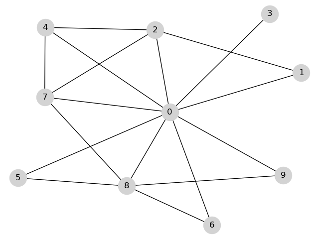
Figure 3: 10-class interference graph.

Throughout this section we focus on the 10-class network displayed in Figure 3 with the following parameters:

$$\lambda_{c}=0.4,\qquad \text{for }c=1,\ldots,9$$

$$\nu_{c}=\mu_{c}=3,\qquad \text{for }c=0,\ldots,9$$

and an equal number of nodes in each class, i.e., $p_{c}=0.1$ for $c=0,\ldots,9$. We let $\lambda_{0}$ vary and consider two scenarios.

In Scenario 1, we set $\lambda_{0}=0.25$, and we verify that $\boldsymbol{\xi}=\boldsymbol{\eta}(\boldsymbol{\rho})<\boldsymbol{e}$ to ensure that a unique fixed point $\boldsymbol{x}^{*}$ of (6) exists, by virtue of Theorem 3.2. In order to solve (33), we use the numerical algorithm described in [12], which is an adaptation of the algorithm presented in [35], and obtain

$$\boldsymbol{\xi}\approx(0.478,\>0.205,\>0.311,\>0.170,\>0.258,\>0.205,\>0.205,\>0.311,\>0.359,\>0.205).$$

Note that $\boldsymbol{\xi}<\boldsymbol{e}$, and Theorem 3.2 thus yields that

$$\boldsymbol{x}^{*}=(x^{*}_{c,n}),\qquad x^{*}_{c,n}=(1-\xi_{c})\xi_{c}^{n},$$

is the unique fixed point.

In Scenario 2, we double the arrival rate at node 0, i.e., $\lambda_{0}=0.5$, and observe that (6) has no fixed points. In fact, by means of the numerical algorithm described in [12] we obtain that

$$\boldsymbol{\xi}\approx(1.317,\>0.235,\>0.380,\>0.190,\>0.308,\>0.235,\>0.235,\>0.380,\>0.443,\>0.235).$$

In this case $\xi_{0}>1$, and in view of Theorem 3.2, no fixed point for (6) exists.

Convergence of the population process to the solution of (6). We first visually illustrate the result stated in Theorem 3.1, i.e, the convergence of the properly scaled population process $\boldsymbol{X}^{(N)}(t)$ to the solution $\boldsymbol{x}(t)$ of (6) for arbitrary interference graphs. In Figure 4 we display sample paths of the scaled population process and compare these with the solution $\boldsymbol{x}(t)$ of (6). We show the results for both Scenarios 1 and 2, and confirm that Theorem 3.1 holds independently of the existence of the fixed point. For both cases we let the number of nodes per class be $100$ or $1000$. Note that the oscillations around $\boldsymbol{x}(t)$ decrease in magnitude as $N$ increases.

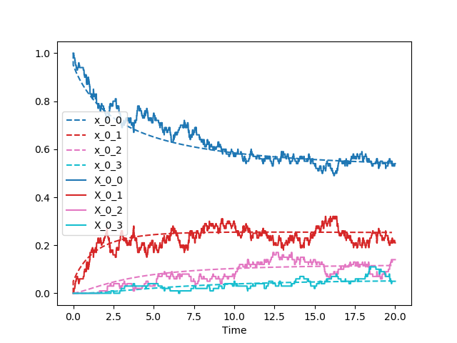
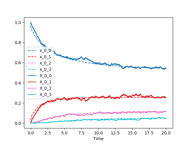
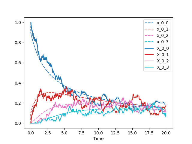
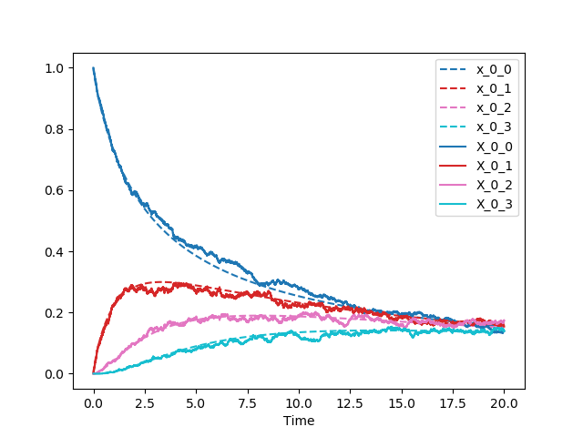
Figure 4: Plot of the sample path $X^{(N)}(Nt)$ and of the solution $x_{c,n}(t)$ of (6) for $c=0$ and $n=0,1,2,3$. Both for Scenario 1 (top) and Scenario 2 (bottom) with $N_{c}=100$ (left) and $N_{c}=1000$ (right).

Scenario 1. Convergence to the fixed point. For Scenario 1 we derived a unique fixed point $\boldsymbol{x}^{*}$ of (6). In Figure 5 we display a numerical solution of (6) with empty initial condition, and observe that $\boldsymbol{x}(t)\rightarrow\boldsymbol{x}^{*}$ as $t\to\infty$. This supports the hypothesis that the solution $\boldsymbol{x}(t)$ converges to $\boldsymbol{x}^{*}$ even when the interference graph is not complete.

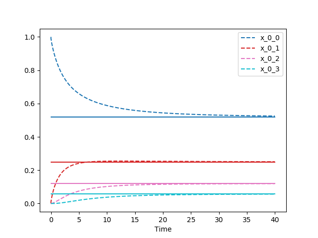
Figure 5: Scenario 1. Plot of the solution $x_{c,n}(t)$ of (6) for $c=0,4$ and $n=0,1,2,3$.

Scenario 2. Explosion of the population process. For Scenario 2 we established that there exists no fixed point of (6). In this case, we observe a dichotomy in behavior. Some classes explode, i.e., the number of backlogged packets in the buffer of every node grows without bound. Other classes remain stable, but the stationary buffer content distribution is no longer geometric with parameters given by the activity factors $\boldsymbol{\xi}$. In Figure 6 we display a numerical solution of (6) with empty initial condition. Observe that for class $0$, the solution is non-monotone and converges to $0$. In contrast, for class $4$, the solution converges to a fixed point which is however no longer characterized by $\boldsymbol{\xi}$ (even if very close).

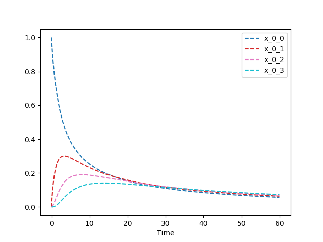
Figure 6: Scenario 2. Plot of the solution $x_{c,n}(t)$ of (6) for $c=0,4$ and $n=0,1,2,3$.

7 Conclusion

We analyzed distributed random-access networks in a many-sources regime with buffer dynamics. The difficulty in the analysis is the complex interaction between the medium activity state and the buffer content process. However, in the mean-field regime, these processes are shown to decouple and a tractable initial-value problem describing the buffer content process is obtained. The methodological framework that we developed is fairly generic, and expected to be applicable to a broader range of problems where a similar decoupling occurs.

For the case of a complete interference graph the stationary buffer content and the packet waiting and sojourn time are shown to converge in distribution and expectation to random variables whose parameters are explicitly given by the unique fixed point of the initial-value problem. These results are obtained via an interchange of limits approach which ensures that the resulting approximations are asymptotically exact. Numerical experiments suggest that these results extend to general interference graphs, but a rigorous proof remains as a challenging problem for further research.

The theoretical machinery for the derivation of mean-field limits developed in Section 4 is highly flexible and may be applied to a wide range of models. The basic model described in Section 2 can be extended, and the associated mean-field limits may be obtained along similar lines. For instance, with minimal additional effort, mean-field limits can be obtained for models with queue-based back-off rates and finite-capacity buffers. The time-scale separation between the activity process and the population process plays a key role once again. However, the expression for the stationary distribution of the activity process with a fixed population is model-dependent, and this is reflected in the corresponding limiting initial-value problems which differ only in the expression for $\pi_{\boldsymbol{x}}(\Omega_{-c})$, see [16] for further details.

Appendix A Extended proofs

A.1 Proof of Lemma 4.4

We already observed that the process ${\boldsymbol{\Xi}}^{(N)}$ is a multi-parameter martingale adapted to a filtration ${\bf F}$. Since $C$ is finite and $\frac{\lvert\Xi^{(N)}_{c,n}(t)\rvert}{1+\lvert\Xi^{(N)}_{c,n}(t)\rvert}\leq 1$ for every $t\geq 0$, there exists $K_{\eta}$ such that

$$\sum_{c\in\mathcal{C}}\sum_{n>K_{\eta}}2^{-n}\frac{\lvert\Xi^{(N)}_{c,n}(t)\rvert}{1+\lvert\Xi^{(N)}_{c,n}(t)\rvert}<\eta/2.$$

For each $c\in\mathcal{C},n\leq K_{\eta}$, $\Xi^{(N)}_{c,n}(t)$ is a ${\cal L}^{2}$ ${\bf F}$ martingale so that $\left(\Xi^{(N)}(t)\right)^{2}$ is a ${\cal L}^{1}$ ${\bf F}$ submartingale. Applying Doob’s submartingale inequality with $p=1$ (see [30]), we obtain

$${\mathbb{P}}\left\{{\displaystyle\sup_{t\in[0,T]}\lvert\Xi^{(N)}_{c,n}(t)\rvert^{2}>\varepsilon}\right\}\leq\frac{{\mathbb{E}}\left\{{\displaystyle\lvert\Xi^{(N)}_{c,n}(T)\rvert^{2}}\right\}}{\epsilon},\qquad c\in\mathcal{C},n\leq K_{\eta}.$$

However ${\mathbb{E}}\left\{{\displaystyle\lvert\Xi^{(N)}_{c,n}(T)\rvert^{2}}\right\}=O(1/N)$ from which the result follows.

A.2 Lipschitz continuity of the function $H(\cdot)$

For simplicity, denote by $\boldsymbol{x}^{(c)}=(x_{c,n})_{n\in\mathbb{N}_{0}}$ and we know that $\boldsymbol{x}^{(c)}\in\chi$ which is closed and compact under the poduct topology. We will leverage the following lemma, whose proof is omitted.

Lemma A.1.

Given $\boldsymbol{f},\boldsymbol{g}:E\rightarrow\prod_{c\in\mathcal{C}}\mathbb{R}^{\infty}$ Lipschitz continuous functions, then so is $\boldsymbol{h}$, where $\boldsymbol{h}(\boldsymbol{x})=\boldsymbol{f}(\boldsymbol{x})+\boldsymbol{g}(\boldsymbol{x})$. Given $f,g:E\rightarrow\mathbb{R}$ Lipschitz continuous and bounded functions, then so is $h$, where $h(\boldsymbol{x}):=f(\boldsymbol{x})g(\boldsymbol{x})$.

Let us recall that

$$\rho\big{(}(\boldsymbol{x}^{(1)},\ldots,\boldsymbol{x}^{(C)}),(\boldsymbol{y}^{(1)},\ldots,\boldsymbol{y}^{(C)})\big{)}=\sum_{c\in\mathcal{C}}\rho_{1}\big{(}\boldsymbol{x}^{(c)},\boldsymbol{y}^{(c)}\big{)}.$$

Note that the first part of function $H(\boldsymbol{x})$, i.e.,

$$\sum_{c\in\mathcal{C}}\frac{1}{p_{c}}\lambda_{c}\sum_{n\in\mathbb{N}_{0}}x_{c,n}\boldsymbol{e}_{n}^{n+1},$$

is clearly Lipschitz. Let us now focus on the second part, for simplicity we neglect the constants $1/p_{c}$ and $\nu_{c}$. Consider the term

$$\pi_{\boldsymbol{x}_{0}}(\Omega_{-c})x_{c,n}$$

for some $c\in\mathcal{C}$. Clearly $x_{c,n}$ is Lipschitz continuous and bounded for every $\boldsymbol{x}^{(c)}\in\chi$, as for the term $\pi_{\boldsymbol{x}_{0}}(\Omega_{-c})$ it is clearly bounded and we now show that it is Lipschitz continuous in $\boldsymbol{x}$. Note that, we can write $\pi_{\boldsymbol{x}_{0}}(\Omega_{-c})$ as

$$\pi_{\boldsymbol{x}_{0}}(\Omega_{-c})=\frac{a^{(c)}(x_{0}^{(1)},\ldots,x_{0}^{(C)})}{b^{(c)}(x_{0}^{(1)},\ldots,x_{0}^{(C)})},$$

where both $a^{(c)}$ and $b^{(c)}$ are polynomials in the variables $\{x^{(c)}_{0}\}_{c\in\mathcal{C}}$ such that

$$a^{(c)}(x_{0}^{(1)},\ldots,x_{0}^{(C)})\geq 0,\qquad b^{(c)}(x_{0}^{(1)},\ldots,x_{0}^{(C)})\geq 1,$$

for every $(\boldsymbol{x}^{(1)},\ldots,\boldsymbol{x}^{(C)})\in E$. Hence, it holds that

$$\frac{\partial a^{(c)}}{\partial x_{0}^{(d)}}=\frac{\partial\pi_{\boldsymbol{x}_{0}}(\Omega_{-c})}{\partial x_{0}^{(d)}}b^{(c)}+\pi_{\boldsymbol{x}_{0}}(\Omega_{-c})\frac{\partial b^{(c)}}{\partial x_{0}^{(d)}}.$$

Observe that $\frac{\partial a^{(c)}}{\partial x_{0}^{(d)}}$ and $\frac{\partial b^{(c)}}{\partial x_{0}^{(d)}}$ are both bounded and continuous, and therefore $\frac{\partial\pi_{\boldsymbol{x}_{0}}(\Omega_{-c})}{\partial x_{0}^{(d)}}$ is bounded as well for every $c,d\in\mathcal{C}$. Since $C$ is finite, there exists $L_{\pi}<\infty$ such that

$$\big{|}\frac{\partial\pi_{\boldsymbol{x}_{0}}(\Omega_{-c})}{\partial x_{0}^{(d)}}\big{|}\leq L_{\pi},\qquad\forall c,d\in\mathcal{C}.$$

Hence, we have that

$$\big{|}\pi_{\boldsymbol{x}_{0}}(\Omega_{-c})-\pi_{\boldsymbol{y}_{0}}(\Omega_{-c})\big{|} \leq L_{\pi}\sum_{d\in\mathcal{C}}|x_{0}^{(d)}-y_{0}^{(d)}|$$

$$\leq L_{\pi}\rho\big{(}(\boldsymbol{x}^{(1)},\ldots,\boldsymbol{x}^{(C)}),(\boldsymbol{y}^{(1)},\ldots,\boldsymbol{y}^{(C)})\big{)},$$

yielding that $\pi_{\boldsymbol{x}_{0}}(\Omega_{-c})$ is Lipschitz continuous in $\boldsymbol{x}\in E$. The above results, together with Lemma A.1, suffice to prove the Lipschitz continuity of function $H(\boldsymbol{x})$.

A.3 Proof of Corollary 4.5

Thanks to the fundamental theorem of calculus applied to (31), it holds that

$$0=\nu_{c}(1-x_{c,0}(t))\sum_{\omega\in\Omega_{-c}}\dot{\alpha}_{\omega}(t)-\mu_{c}\sum_{\omega\in\Omega_{+c}}\dot{\alpha}_{\omega}(t),\qquad\text{a.e.}$$ (43)

Hence, at every time $t$, we have to look for solutions $(z^{t}_{\omega})_{\omega\in\Omega}$ of

$$\nu_{c}(1-x_{c,0}(t))\sum_{\omega\in\Omega_{-c}}z_{\omega}^{t}=\mu_{c}\sum_{\omega\in\Omega_{+c}}z_{\omega}^{t},\quad\forall c\in\mathcal{C},$$ (44)

where in view of (29) $\sum_{\omega\in\Omega}z_{\omega}^{t}=1$ and $z_{\omega}^{t}\geq 0$. Observe that, $z_{\omega}^{t}$ corresponds to the stationary fraction of time spent by the activity process in state $\omega\in\Omega$ in the saturated network where node $c$ transmits at rate $\mu_{c}$ and back-offs at rate $\nu_{c}(1-x_{c,0}(t))$, i.e.,

$$\dot{\alpha}_{\omega}(t)=z_{\omega}^{t}=\pi(\omega;\boldsymbol{e}-\boldsymbol{x}_{0}(t))=\pi_{\boldsymbol{x}_{0}(t)}(\omega).$$

In particular, existence and uniqueness of the stationary distribution $\pi_{\boldsymbol{x}_{0}(t)}(\omega)$ is ensured whenever $\boldsymbol{x}_{0}(t)\leq\boldsymbol{e}$. Hence, $\dot{\alpha}_{\omega}(t)=z^{t}_{\omega}$ is well-defined and, since an increasing unit Lipschitz function starting from $0$ is determined by its derivatives, the equality holds for all $t$, determining $\alpha_{\omega}$. Observe that $\alpha_{\omega}$ exists everywhere since it coincides with the integral of a continuous function.

A.4 Proof of Proposition 5.4

Given the sequence of stationary distributions of the population process $\{\pi_{\boldsymbol{X}_{*}^{(N)}}\}_{N\geq 1}$, we will show that for every $\epsilon>0$ there exist a compact set $\mathcal{K}_{\epsilon}\subset E^{1}$ and $N_{\epsilon}>0$ such that

$$\mathbb{P}\big{\{}\boldsymbol{X}^{(N)}\in\mathcal{K}_{\epsilon}\big{\}}>1-\epsilon,\qquad\forall\>N>N_{\epsilon}.$$ (45)

In particular, we will show that the above relation holds for a compact set $\mathcal{K}_{\epsilon}$ defined as

$$\mathcal{K}_{\epsilon}=\big{\{}\boldsymbol{x}\in E^{1}:\sum_{c\in\mathcal{C}}m_{c}(\boldsymbol{x})\leq K_{\epsilon}\big{\}}.$$

Let us now show that $\mathcal{K}_{\epsilon}$ is compact. Note that $\mathcal{K}_{\epsilon}\subseteq E$, which is compact. Hence, it is sufficient to prove that $\mathcal{K}_{\epsilon}$ is closed. Observe that any sequence $\boldsymbol{x}_{n}$ in $\mathcal{K}_{\epsilon}$ is also a sequence in $E$. Let $\boldsymbol{x}$ be a limit point of this sequence which is necessarily in $E$. But clearly

$$\sum_{c\in\mathcal{C}}m_{c}({\boldsymbol{x}}_{n})\leq K_{\epsilon},\qquad\forall n$$

and $\boldsymbol{x}_{n}$ is a vector of probabilities on $\mathbb{N}_{0}$ with $C$ components. It follows that each component sequence is tight and therefore the limit must be in $E^{1}$. Now let $\mu_{c}$ be the expectation of the limit (possibly infinite). Then, from [4, Theorem 5.3, p. 32], we know that

$$\mu_{c}\leq\liminf m_{c}({\bf x}_{n})\leq K_{\epsilon}.$$

Since $\sum_{c}\mu_{c}\leq\sum_{c}\liminf m_{c}({\boldsymbol{x}}_{n})\leq\liminf\sum_{c}m_{c}({\boldsymbol{x}}_{n})\leq K_{\epsilon}$ the required bound on the sum expectations holds and so the limit is in $\mathcal{K}_{\epsilon}$, which is therefore closed.

Note that

$$\mathbb{P}\big{\{}\boldsymbol{X}_{*}^{(N)}\notin\mathcal{K}_{\epsilon}\big{\}}=\mathbb{P}\big{\{}\sum_{c\in\mathcal{C}}m_{c}(\boldsymbol{X}_{*}^{(N)})>K_{\epsilon}\big{\}}\leq\frac{\sum_{c\in\mathcal{C}}\mathbb{E}\Big{[}m_{c}(\boldsymbol{X}_{*}^{(N)})\Big{]}}{K_{\epsilon}},$$

due to Markov’s inequality.

Consider class $c\in\mathcal{C}$. Let $Q_{c,k}^{(N)}$ be the random variable denoting the number of packets waiting in the buffer of the $k$-th class-$c$ node in stationarity. Note that $Q_{c,k}^{(N)}=Q_{c}^{(N)}$ for every $k\in\{1,\ldots,N_{c}\}$, due to the exchangeability of the nodes within the same class, and observe that

$$\mathbb{E}[Q_{c}^{(N)}] =\sum_{\boldsymbol{q}\in\mathbb{N}_{0}^{N}}\pi_{\boldsymbol{Q}^{(N)}}(\boldsymbol{q})\frac{1}{N_{c}}\sum_{k=1}^{N_{c}}q_{c,k}$$

$$=\sum_{\boldsymbol{q}\in\mathbb{N}_{0}^{N}}\pi_{\boldsymbol{Q}^{(N)}}(\boldsymbol{q})\frac{1}{N_{c}}\sum_{k=1}^{N_{c}}\sum_{n=1}^{\infty}n\mathbbm{1}\{q_{c,k}=n\}$$

$$=\sum_{\boldsymbol{x}\in E^{1}}\pi_{\boldsymbol{X}_{*}^{(N)}}(\boldsymbol{x})\sum_{n=1}^{\infty}nx_{c,n}=\mathbb{E}\big{[}m_{c}(\boldsymbol{X}_{*}^{(N)})\big{]},$$

where the second equality is due to (40). Hence,

$$\mathbb{P}\big{\{}\boldsymbol{X}_{*}^{(N)}\notin\mathcal{K}_{\epsilon}\big{\}}\leq\frac{\sum_{c\in\mathcal{C}}\mathbb{E}[Q_{c}^{(N)}]}{K_{\epsilon}}.$$ (46)

For every class $c\in\mathcal{C}$, by neglecting the time periods in which class-$c$ nodes cannot activiate due to activity of their neighbors, we obtain that

$$\big{(}\frac{1}{\mu_{c}}+\frac{N_{c}}{\nu_{c}}\big{)}\mathbb{E}[Q^{(N)}_{c}]\leq\mathbb{E}[W^{(N)}_{c}],$$

and therefore

$$\sum_{c\in\mathcal{C}}\mathbb{E}[Q^{(N)}_{c}]\leq\sum_{c\in\mathcal{C}}\big{(}\frac{1}{\mu_{c}}+\frac{N_{c}}{\nu_{c}}\big{)}^{-1}\mathbb{E}[W^{(N)}_{c}]\leq\sum_{c\in\mathcal{C}}\frac{\nu_{c}}{N_{c}}\mathbb{E}[W^{(N)}_{c}].$$ (47)

Thus, it suffices to show that $\mathbb{E}[W^{(N)}_{c}]$ grows at most linearly in $N$ as $N\rightarrow\infty$.

Combining (46) and (47), we obtain

$$\mathbb{P}\big{\{}\boldsymbol{X}_{*}^{(N)}\notin\mathcal{K}_{\epsilon}\big{\}}\leq\frac{1}{K_{\epsilon}}\sum_{c\in\mathcal{C}}\frac{\nu_{c}}{N_{c}}\mathbb{E}[W_{c}^{(N)}].$$

In view of (39), for any $\epsilon>0$ we can therefore pick $K_{\epsilon}$ such that (45) is asymptotically satisfied.

References

• [1] L. Atzori, A. Iera, G. Morabito (2010). The Internet of Things: a survey. Computer Networks 54 (15), 2787–2805.
• [2] D. Bertsimas, D. Nazakato (1995). The distributional Little’s law and its applications. Operations Research 43 (2), 298–310.
• [3] G. Bianchi (2000). Performance analysis of the IEEE 802.11 distributed coordination function. IEEE Journal on Selected Areas in Communications 18 (3), 535–547.
• [4] P. Billingsley (1968). Convergence of Probability Measures. 1st Edition.
• [5] P. Billingsley (1999). Convergence of Probability Measures. 2nd Edition.
• [6] R.R. Boorstyn, A. Kershenbaum, B. Maglaris, V. Sahin (1987). Throughput analysis in multihop CSMA packet radio networks. IEEE Transactions on Communications 35, 267–274.
• [7] C. Bordenave, D. McDonald, A. Proutiere (2008). Performance of random medium access control, an asymptotic approach. ACM SIGMETRICS Performance Evaluation Review 36 (1), 1–12.
• [8] O.J. Boxma, J.A. Weststrate (1989). Waiting times in polling systems with Markovian server routing. In: Proc. Messung, Modellierung und Bewertung von Rechensystemen und Netzen. 89–105.
• [9] M. Bramson (1998). State space collapse with application to heavy traffic limits for multiclass queueing networks. Queueing Systems 30 (1-2), 89–140.
• [10] F. Cecchi (2018). Mean-field limits for ultra-dense random-access networks. PhD Thesis. Eindhoven University of Technology
• [11] F. Cecchi, S.C. Borst, J.S.H. van Leeuwaarden (2014). Throughput of CSMA networks with buffer dynamics. Performance Evaluation 79, 216–234.
• [12] F. Cecchi, S.C. Borst, J.S.H. van Leeuwaarden, P.A. Whiting (2016). CSMA networks in a many-sources regime: A mean-field approach. In: Proc. IEEE Infocom.
• [13] J. Cho, J.Y. Le Boudec, Y. Jiang (2012). On the asymptotic validity of the decoupling assumption for analyzing 802.11 MAC protocol. IEEE Transactions on Information Theory 58 (11), 6879–6893.
• [14] J.G. Dai, S.P. Meyn (1995). Stability and convergence of moments for multiclass queueing networks via fluid limit models. IEEE Transactions on Automatic Control 40 (11), 1889–1904.
• [15] F.S. De Biasi, G. Pianigiani (1986). Uniqueness for differential equations implies continuous dependence only in finite dimension. Bulletin of the London Mathematical Society 18 (4), 379–382.
• [16] F. Cecchi (2018). Mean-field Limits for Ultra-Dense Random-Access Networks. PhD Thesis Eindhoven University of Technology.
• [17] D. Down (1998). On the stability of polling models with multiple servers. Journal of Applied Probability 34 (4), 925–935.
• [18] K.R. Duffy (2010). Mean field Markov models of wireless local area networks. Markov Processes and Related Fields 16 (2), 295–328.
• [19] S.N. Ethier, T.G. Kurtz (1986). Markov Processes: Characterization and Convergence.
• [20] D. Evans (2011). The internet of things. How the next evolution of the internet is changing everything, Whitepaper, Cisco (IBSG).
• [21] M. Feuillet, P. Robert (2014). A scaling analysis of a transient stochastic network. Advances in Applied Probability 46 (2), 516–535.
• [22] C. Fricker, M.R. Jaibi (1998). Stability of multi-server polling models. INRIA Research report, No. 3347.
• [23] D. Gamarnik, A. Zeevi (2006). Validity of heavy traffic steady-state approximations in generalized Jackson networks. Annals of Applied Probability 16 (1), 56–90.
• [24] M. Halldorsson, T. Tonoyan (2015). How well can graphs represent wireless interference? In: Proc. ACM Symposium on Theory of Computing.
• [25] P.J. Hunt, T.G. Kurtz (1994). Large loss networks. Stochastic Processes and their Applications 53 (2), 363–378.
• [26] L. Jiang, J. Walrand (2008). A distributed CSMA algorithm for throughput and utility maximization in wireless networks. In: Proc. Allerton Conference, 1511–1519.
• [27] W. Kang, K. Ramanan (2012). Asymptotic approximations for stationary distributions of many-server queues with abandonment. Annals of Applied Probability 22 (2), 477–521.
• [28] T.G. Kurtz (1980). Representations of Markov processes as multiparameter time changes. Annals of Applied Probability 8 (4), 682–715.
• [29] S.C. Liew, C.H. Kai, J. Leung, B. Wong (2010). Back-of-the-envelope computation of throughput distributions in CSMA wireless networks. IEEE Transactions on Mobile Computing 9 (9), 1319–1331.
• [30] D. Revuz, M. Yor (2013). Continuous Martingales and Brownian Motion.
• [31] W. Rudin (1976). Principles of mathematical analysis. 3rd Edition.
• [32] G. Sharma, A. Ganesh, P.B. Key (2009). Performance analysis of contention based medium access control protocols. IEEE Transactions on Information Theory 55 (4), 1665–1682.
• [33] A. Stolyar (2005). On the asymptotic optimality of the gradient scheduling algorithm for multiuser throughput allocation. Operations Research 53 (1), 12–25.
• [34] P.M. van de Ven, S.C. Borst, J.S.H. van Leeuwaarden, A. Proutiere (2010). Insensitivity and stability of random-access networks. Performance Evaluation 67 (11), 1230–1242.
• [35] P.M. van de Ven, A.J.E.M. Janssen, J.S.H. van Leeuwaarden, S.C. Borst (2011). Achieving target throughputs in random-access networks. Performance Evaluation 68 (11), 1103–1117.
• [36] X. Wang, K. Kar (2005). Throughput modeling and fairness issues in CSMA/CA based ad-hoc networks. In: Proc. IEEE Infocom.
• [37] W. Whitt (1985). Blocking when service is required from several facilities simultaneously. AT&T Technical Journal 64 (8), 1807–1856.
• [38] W. Whitt (1969). Weak convergence of probability measures on the function space $C[0,\infty)$. Technical Report No. 120, Stanford University.
• [39] W. Whitt (1970). Weak convergence of probability measures on the function space $C[0,\infty)$. The Annals of Mathematical Statistics 41 (3), 939–944.
• [40] X. Zhou, Z. Zhang, G. Wang, X. Yu, B.Y. Zhao, H. Zheng (2013). Practical conflict graphs for dynamic spectrum distribution. In: Proc. ACM SIGMETRICS 41 (1), 5–16.