Efficient Linear Programming for Dense CRFs

Abstract

The fully connected conditional random field (CRF) with Gaussian pairwise potentials has proven popular and effective for multi-class semantic segmentation. While the energy of a dense CRF can be minimized accurately using a linear programming (LP) relaxation, the state-of-the-art algorithm is too slow to be useful in practice. To alleviate this deficiency, we introduce an efficient LP minimization algorithm for dense CRFs. To this end, we develop a proximal minimization framework, where the dual of each proximal problem is optimized via block coordinate descent. We show that each block of variables can be efficiently optimized. Specifically, for one block, the problem decomposes into significantly smaller subproblems, each of which is defined over a single pixel. For the other block, the problem is optimized via conditional gradient descent. This has two advantages: 1) the conditional gradient can be computed in a time linear in the number of pixels and labels; and 2) the optimal step size can be computed analytically. Our experiments on standard datasets provide compelling evidence that our approach outperforms all existing baselines including the previous LP based approach for dense CRFs.

1 Introduction

In the past few years, the dense conditional random field (CRF) with Gaussian pairwise potentials has become popular for multi-class image-based semantic segmentation. At the origin of this popularity lies the use of an efficient filtering method [1], which was shown to lead to a linear time mean-field inference strategy [12]. Recently, this filtering method was exploited to minimize the dense CRF energy using other, typically more effective, continuous relaxation methods [6]. Among the relaxations considered in [6], the linear programming (LP) relaxation provides strong theoretical guarantees on the quality of the solution [9, 15].

In [6], the LP was minimized via projected subgradient descent. While relying on the filtering method, computing the subgradient was shown to be linearithmic in the number of pixels, but not linear. Moreover, even with the use of a line search strategy, the algorithm required a large number of iterations to converge, making it inefficient.

We introduce an iterative LP minimization algorithm for a dense CRF with Gaussian pairwise potentials which has linear time complexity per iteration. To this end, instead of relying on a standard subgradient technique, we propose to make use of the proximal method [19]. The resulting proximal problem has a smooth dual, which can be efficiently optimized using block coordinate descent. We show that each block of variables can be optimized efficiently. Specifically, for one block, the problem decomposes into significantly smaller subproblems, each of which is defined over a single pixel. For the other block, the problem can be optimized via the Frank-Wolfe algorithm [8, 16]. We show that the conditional gradient required by this algorithm can be computed efficiently. In particular, we modify the filtering method of [1] such that the conditional gradient can be computed in a time linear in the number of pixels and labels. Besides this linear complexity, our approach has two additional benefits. First, it can be initialized with the solution of a faster, less accurate algorithm, such as mean-field [12] or the difference of convex (DC) relaxation of [6], thus speeding up convergence. Second, the optimal step size of our iterative procedure can be obtained analytically, thus preventing the need to rely on an expensive line search procedure.

We demonstrate the effectiveness of our algorithm on the MSRC and Pascal VOC 2010 [7] segmentation datasets. The experiments evidence that our algorithm is significantly faster than the state-of-the-art LP minimization technique of [6]. Furthermore, it yields assignments whose energies are much lower than those obtained by other competing methods [6, 12]. Altogether, our framework constitutes the first efficient and effective minimization algorithm for dense CRFs with Gaussian pairwise potentials.

2 Preliminaries

Before introducing our method, let us first provide some background on the dense CRF model and its LP relaxation.

Dense CRF energy function.

A dense CRF is defined on a set of $n$ random variables $\mathcal{X}=\{X_{1},\ldots,X_{n}\}$, where each random variable $X_{a}$ takes a label $x_{a}\in\mathcal{L}$, with $|\mathcal{L}|=m$. For a given labelling $\mathbf{x}$, the energy associated with a pairwise dense CRF can be expressed as

$$E(\mathbf{x})=\sum_{a=1}^{n}\phi_{a}(x_{a})+\sum_{a=1}^{n}\sum_{\begin{subarray}{c}b=1\\ b\neq a\end{subarray}}^{n}\psi_{ab}(x_{a},x_{b})\ ,$$ (1)

where $\phi_{a}$ and $\psi_{ab}$ denote the unary potentials and pairwise potentials, respectively. The unary potentials define the data cost and the pairwise potentials the smoothness cost.

Gaussian pairwise potentials.

Similarly to [6, 12], we consider Gaussian pairwise potentials, which have the following form:

$$\psi_{ab}(x_{a},x_{b}) =\mu(x_{a},x_{b})\sum_{c}w^{(c)}\,k\left(\mathbf{f}_{a}^{(c)},\mathbf{f}_{b}^{(c)}\right)\ ,$$ (2)

$$k(\mathbf{f}_{a},\mathbf{f}_{b}) =\exp\left(\frac{-\|\mathbf{f}_{a}-\mathbf{f}_{b}\|^{2}}{2}\right)\ .$$

Here, $\mu(x_{a},x_{b})$ is referred to as the label compatibility function and the mixture of Gaussian kernels as the pixel compatibility function. The weights $w^{(c)}$ define the mixture coefficients, and $\mathbf{f}_{a}^{(c)}\in\rm I\!R^{d^{(c)}}$ encodes features associated to the random variable $X_{a}$, where $d^{(c)}$ is the feature dimension. For semantic segmentation, each pixel in an image corresponds to a random variable. In practice, as in [6, 12], we then use the position and RGB values of a pixel as features, and assume the label compatibility function to be the Potts model, that is, $\mu(x_{a},x_{b})=\mathbbm{1}[x_{a}\neq x_{b}]$. These potentials proved to be useful in obtaining fine grained labellings in segmentation tasks [12].

Integer programming formulation.

An alternative way of representing a labelling is by defining indicator variables $y_{a:i}\in\{0,1\}$, where $y_{a:i}=1$ if and only if $x_{a}=i$. Using this notation, the energy minimization problem can be written as the following Integer Program (IP):

$$\underset{\mathbf{y}}{\operatorname{\min}}\quad E(\mathbf{y}) =\sum_{a}\sum_{i}\phi_{a:i}\,y_{a:i}+\sum_{a,b\neq a}\sum_{i,j}\psi_{ab:ij}\,y_{a:i}\,y_{b:j}\ ,$$ (3)

$$\text{s.t.}\quad\sum_{i}y_{a:i} =1\quad\quad\ \ \ \forall\,a\in\{1\ldots n\}\ ,$$

$$\hskip 34.69038pty_{a:i} \in\{0,1\}\quad\forall\,a\in\{1\ldots n\},\quad\forall\,i\in\mathcal{L}\ .$$

Here, we use the shorthand $\phi_{a:i}=\phi_{a}(i)$ and $\psi_{ab:ij}=\psi_{ab}(i,j)$. The first set of constraints ensure that each random variable is assigned exactly one label. Note that the value of objective function is equal to the energy of the labelling encoded by $\mathbf{y}$.

Linear programming relaxation.

By relaxing the binary constraints of the indicator variables in (3) and using the fact that the label compatibility function is the Potts model, the linear programming relaxation [9] of (3) is defined as

$$\underset{\mathbf{y}}{\operatorname{\min}}\quad\tilde{E}(\mathbf{y}) =\sum_{a}\sum_{i}\phi_{a:i}\,y_{a:i}+\sum_{a,b\neq a}\sum_{i}K_{ab}\frac{|y_{a:i}-y_{b:i}|}{2}\ ,$$ (4)

$$\text{s.t.}\quad\mathbf{y}\in\mathcal{M} =\left\{\begin{array}[]{l|l}\hbox{\multirowsetup$\mathbf{y}$}&\sum_{i}y_{a:i}=1,\,a\in\{1\ldots n\}\\ &y_{a:i}\geq 0,\,a\in\{1\ldots n\},\,i\in\mathcal{L}\end{array}\right\}\ ,$$ (7)

where $K_{ab}=\sum_{c}w^{(c)}\,k\left(\mathbf{f}_{a}^{(c)},\mathbf{f}_{b}^{(c)}\right)$. For integer labellings, the LP objective $\tilde{E}(\mathbf{y})$ has the same value as the IP objective $E(\mathbf{y})$. It is also worth noting that this LP relaxation is known to provide the best theoretical bounds [9]. Using standard solvers to minimize this LP would require the introduction of $\mathcal{O}(n^{2})$ variables, making it intractable. Therefore the non-smooth objective of Eq. (4) has to be optimized directly. This was handled using projected subgradient descent in [6], which also turns out to be inefficient in practice. In this paper, we introduce an efficient algorithm to tackle this problem while maintaining linear scaling in both space and time complexity.

3 Proximal minimization for LP relaxation

Our goal is to design an efficient minimization strategy for the LP relaxation in (4). To this end, we propose to use the proximal minimization algorithm [19]. This guarantees monotonic decrease in the objective value, enabling us to leverage faster, less accurate methods for initialization. Furthermore, the additional quadratic regularization term makes the dual problem smooth, enabling the use of more sophisticated optimization methods. In the remainder of this paper, we detail this approach and show that each iteration has linear time complexity. In practice, our algorithm converges in a small number of iterations, thereby making the overall approach computationally efficient.

The proximal minimization algorithm [19] is an iterative method that, given the current estimate of the solution $\mathbf{y}^{k}$, solves the problem

$$\underset{\mathbf{y}}{\operatorname{\min}}\quad \tilde{E}(\mathbf{y})+\frac{1}{2\lambda}\left\|\mathbf{y}-\mathbf{y}^{k}\right\|^{2}\ ,$$ (8)

s.t. $$\mathbf{y}\in\mathcal{M}\ ,$$

where $\lambda$ sets the strength of the proximal term.

Note that (8) consists of piecewise linear terms and a quadratic regularization term. Specifically, the piecewise linear term comes from the pairwise term $|y_{a:i}-y_{b:i}|$ in (4) that can be reformulated as $\max\{y_{a:i}-y_{b:i},y_{b:i}-y_{a:i}\}$. The proximal term $\|\mathbf{y}-\mathbf{y}^{k}\|^{2}$ provides the quadratic regularization. In this section, we introduce a new algorithm that is tailored to this problem. In particular, we optimally solve the Lagrange dual of (8) in a block-wise fashion.

Algorithm 1 Proximal minimization of LP

Initial solution $\mathbf{y}^{0}\in\mathcal{M}$ and the dual objective $g$

for $k\leftarrow 0\ldots K$ do

     $A\boldsymbol{\alpha}^{0}\leftarrow\boldsymbol{0},\quad\boldsymbol{\beta}^{0}\leftarrow\boldsymbol{0},\quad\boldsymbol{\gamma}^{0}\leftarrow\boldsymbol{0}$ $\triangleright$ Feasible initialization

     for $t\leftarrow 0\ldots T$ do

         $\left(\boldsymbol{\beta}^{t},\boldsymbol{\gamma}^{t}\right)\leftarrow\underset{\boldsymbol{\beta},\boldsymbol{\gamma}}{\operatorname{argmin}}\,g\left(\boldsymbol{\alpha}^{t},\boldsymbol{\beta},\boldsymbol{\gamma}\right)$ $\triangleright$ Sec. 3.2.1

         $\tilde{\mathbf{y}}^{t}\leftarrow\lambda\left(A\boldsymbol{\alpha}^{t}+B\boldsymbol{\beta}^{t}+\boldsymbol{\gamma}^{t}-\boldsymbol{\phi}\right)+\mathbf{y}^{k}$ $\triangleright$ Current primal solution, may be infeasible

         $A\mathbf{s}^{t}\leftarrow$ conditional gradient of $g$, computed using $\tilde{\mathbf{y}}^{t}$ $\triangleright$ Sec. 3.2.2

         $\delta\leftarrow$ optimal step size given $\left(\mathbf{s}^{t},\boldsymbol{\alpha}^{t},\tilde{\mathbf{y}}^{t}\right)$ $\triangleright$ Sec. 3.2.2

         $A\boldsymbol{\alpha}^{t+1}\leftarrow(1-\delta)A\boldsymbol{\alpha}^{t}+\delta A\mathbf{s}^{t}$ $\triangleright$ Frank-Wolfe update on $\boldsymbol{\alpha}$      

     $\mathbf{y}^{k+1}\leftarrow P_{\mathcal{M}}\left(\tilde{\mathbf{y}}^{t}\right)$ $\triangleright$ Project the primal solution to the feasible set $\mathcal{M}$

3.1 Dual formulation

Let us first write the proximal problem (8) in the standard form by introducing auxiliary variables $z_{ab:i}$.

$$\underset{\mathbf{y},\mathbf{z}}{\operatorname{min}}\quad\sum_{a} \sum_{i}\phi_{a:i}\,y_{a:i}+\sum_{a,b\neq a}\sum_{i}\frac{K_{ab}}{2}z_{ab:i}+\frac{1}{2\lambda}\|\mathbf{y}-\mathbf{y}^{k}\|^{2}\ ,$$ (9a)

$$\text{s.t.}\quad z_{ab:i} \geq y_{a:i}-y_{b:i}\quad\forall\,a\neq b\quad\forall\,i\in\mathcal{L}\ ,$$ (9b)

$$\hskip 19.08203ptz_{ab:i} \geq y_{b:i}-y_{a:i}\quad\forall\,a\neq b\quad\forall\,i\in\mathcal{L}\ ,$$ (9c)

$$\hskip 6.50403pt\sum_{i}y_{a:i} =1\quad\forall\,a\in\{1\ldots n\}\ ,$$ (9d)

$$\hskip 21.68231pty_{a:i} \geq 0\quad\forall\,a\in\{1\ldots n\}\quad\forall\,i\in\mathcal{L}\ .$$ (9e)

We introduce three blocks of dual variables. Namely, $\boldsymbol{\alpha}=\{\alpha^{1}_{ab:i},\alpha^{2}_{ab:i}\mid a\neq b,i\in\mathcal{L}\}$ for the constraints in Eqs. (9b) and (9c), $\boldsymbol{\beta}=\{\beta_{a}\mid a\in\{1\ldots n\}\}$ for Eq. (9d) and $\boldsymbol{\gamma}=\{\gamma_{a:i}\mid a\in\{1\ldots n\},i\in\mathcal{L}\}$ for Eq. (9e), respectively. The vector $\boldsymbol{\alpha}$ has $p=2n(n-1)m$ elements. Here, we introduce two matrices that will be useful to write the dual problem compactly.

Definition 3.1.

Let $A\in\rm I\!R^{nm\times p}$ and $B\in\rm I\!R^{nm\times n}$ be two matrices such that

$$\left(A\boldsymbol{\alpha}\right)_{a:i} =-\sum_{b\neq a}\left(\alpha^{1}_{ab:i}-\alpha^{2}_{ab:i}+\alpha^{2}_{ba:i}-\alpha^{1}_{ba:i}\right)\ ,$$ (10)

$$\left(B\boldsymbol{\beta}\right)_{a:i} =\beta_{a}\ .$$

We can now state our first proposition.

Proposition 3.1.

Given matrices $A\in\rm I\!R^{nm\times p}$ and $B\in\rm I\!R^{nm\times n}$ and dual variables $(\boldsymbol{\alpha},\boldsymbol{\beta},\boldsymbol{\gamma})$.

1. The Lagrange dual of (9a) takes the following form:

   $$\underset{\boldsymbol{\alpha},\boldsymbol{\beta},\boldsymbol{\gamma}}{\operatorname{min}}\ g(\boldsymbol{\alpha},\boldsymbol{\beta},\boldsymbol{\gamma}) =\frac{\lambda}{2}\|A\boldsymbol{\alpha}+B\boldsymbol{\beta}+\boldsymbol{\gamma}-\boldsymbol{\phi}\|^{2}+\left\langle A\boldsymbol{\alpha}+B\boldsymbol{\beta}+\boldsymbol{\gamma}-\boldsymbol{\phi},\mathbf{y}^{k}\right\rangle-\langle\boldsymbol{1},\boldsymbol{\beta}\rangle\ ,$$ (11)

   $$\text{s.t.}\hskip 34.69038pt\gamma_{a:i} \geq 0\quad\forall\,a\in\{1\ldots n\}\quad\forall\,i\in\mathcal{L}\ ,$$

   $$\hskip 34.69038pt\boldsymbol{\alpha}\in\mathcal{C} =\left\{\begin{array}[]{l|l}\hbox{\multirowsetup$\boldsymbol{\alpha}$}&\alpha^{1}_{ab:i}+\alpha^{2}_{ab:i}=\frac{K_{ab}}{2},\,\forall\,a\neq b,\,\forall\,i\in\mathcal{L}\\ &\alpha^{1}_{ab:i},\alpha^{2}_{ab:i}\geq 0,\,\forall\,a\neq b,\,\forall\,i\in\mathcal{L}\end{array}\right\}\ .$$ (14)

2. The primal variables $\mathbf{y}$ satisfy

   $$\mathbf{y}=\lambda\left(A\boldsymbol{\alpha}+B\boldsymbol{\beta}+\boldsymbol{\gamma}-\boldsymbol{\phi}\right)+\mathbf{y}^{k}\ .$$ (15)

Proof.

In Appendix A.1. ∎

3.2 Algorithm

The dual problem (11), in its standard form, can only be tackled using projected gradient descent. However, by separating the variables based on the type of the feasible domains, we propose an efficient block coordinate descent approach. Each of these blocks are amenable to more sophisticated optimization, resulting in a computationally efficient algorithm. As the dual problem is strictly convex and smooth, the optimal solution is still guaranteed. For $\boldsymbol{\beta}$ and $\boldsymbol{\gamma}$, the problem decomposes over the pixels, as shown in 3.2.1, therefore making it efficient. The minimization with respect to $\boldsymbol{\alpha}$ is over a compact domain, which can be efficiently tackled using the Frank-Wolfe algorithm [8, 16]. Our complete algorithm is summarized in Algorithm 1. In the following sections, we discuss each step in more detail.

3.2.1 Optimizing over $\boldsymbol{\beta}$ and $\boldsymbol{\gamma}$

We first turn to the problem of optimizing over $\boldsymbol{\beta}$ and $\boldsymbol{\gamma}$ while $\boldsymbol{\alpha}^{t}$ is fixed. Since the dual variable $\boldsymbol{\beta}$ is unconstrained, the minimum value of the dual objective $g$ is attained when $\nabla_{\boldsymbol{\beta}}g(\boldsymbol{\alpha}^{t},\boldsymbol{\beta},\boldsymbol{\gamma})=0$.

Proposition 3.2.

If $\nabla_{\boldsymbol{\beta}}g(\boldsymbol{\alpha}^{t},\boldsymbol{\beta},\boldsymbol{\gamma})=0$, then $\boldsymbol{\beta}$ satisfy

$$\boldsymbol{\beta}=B^{T}\left(A\boldsymbol{\alpha}^{t}+\boldsymbol{\gamma}-\boldsymbol{\phi}\right)/m\ .$$ (16)

Proof.

More details on the simplification is given in Appendix A.2. ∎

Note that, now, $\boldsymbol{\beta}$ is a function of $\boldsymbol{\gamma}$. We therefore substitute $\boldsymbol{\beta}$ in (11) and minimize over $\boldsymbol{\gamma}$. Interestingly, the resulting problem can be optimized independently for each pixel, with each subproblem being an $m$ dimensional quadratic program (QP) with nonnegativity constraints, where $m$ is the number of labels.

Proposition 3.3.

The optimization over $\boldsymbol{\gamma}$ decomposes over pixels where for a pixel $a$, this QP has the form

$$\underset{\boldsymbol{\gamma}_{a}}{\operatorname{\min}}\quad \frac{1}{2}\boldsymbol{\gamma}^{T}_{a}Q\boldsymbol{\gamma}_{a}+\left\langle\boldsymbol{\gamma}_{a},Q\left((A\boldsymbol{\alpha}^{t})_{a}-\boldsymbol{\phi}_{a}\right)+\mathbf{y}^{k}_{a}\right\rangle\ ,$$ (17)

s.t. $$\boldsymbol{\gamma}_{a}\geq\boldsymbol{0}\ .$$

Here, $\boldsymbol{\gamma}_{a}$ denotes the vector $\{\gamma_{a:i}\mid i\in\mathcal{L}\}$ and $Q=\lambda\left(I-\boldsymbol{1}/m\right)\in\rm I\!R^{m\times m}$, with $I$ the identity matrix and $\boldsymbol{1}$ the matrix of all ones.

Proof.

In Appendix A.2. ∎

We use the algorithm of [26] to efficiently optimize every such QP. In our case, due to the structure of the matrix $Q$, the time complexity of an iteration is linear in the number of labels. Hence, the overall time complexity of optimizing over $\boldsymbol{\gamma}$ is $\mathcal{O}(nm)$. Once the optimal $\boldsymbol{\gamma}$ is computed for a given $\boldsymbol{\alpha}^{t}$, the corresponding optimal $\boldsymbol{\beta}$ is given by Eq. (16).

3.2.2 Optimizing over $\boldsymbol{\alpha}$

We now turn to the problem of optimizing over $\boldsymbol{\alpha}$ given $\boldsymbol{\beta}^{t}$ and $\boldsymbol{\gamma}^{t}$. To this end, we use the Frank-Wolfe algorithm [8], which has the advantage of being projection free. Furthermore, for our specific problem, we show that the required conditional gradient can be computed efficiently and the optimal step size can be obtained analytically.

Conditional gradient computation.

The conditional gradient with respect to $\boldsymbol{\alpha}$ is obtained by solving the following linearization problem

$$\mathbf{s}=\underset{\hat{\mathbf{s}}\in\mathcal{C}}{\operatorname{argmin}}\,\left\langle\hat{\mathbf{s}},\nabla_{\boldsymbol{\alpha}}g(\boldsymbol{\alpha}^{t},\boldsymbol{\beta}^{t},\boldsymbol{\gamma}^{t})\right\rangle\ .$$ (18)

Here, $\nabla_{\boldsymbol{\alpha}}g(\boldsymbol{\alpha}^{t},\boldsymbol{\beta}^{t},\boldsymbol{\gamma}^{t})$ denotes the gradient of the dual objective function with respect to $\boldsymbol{\alpha}$ evaluated at $(\boldsymbol{\alpha}^{t},\boldsymbol{\beta}^{t},\boldsymbol{\gamma}^{t})$.

Proposition 3.4.

The conditional gradient $\mathbf{s}$ satisfy

$$\left(A\mathbf{s}\right)_{a:i}=-\sum_{b}\left(K_{ab}\mathbbm{1}[\tilde{y}^{t}_{a:i}\geq\tilde{y}^{t}_{b:i}]-K_{ab}\mathbbm{1}[\tilde{y}^{t}_{a:i}\leq\tilde{y}^{t}_{b:i}]\right)\ ,$$ (19)

where $\tilde{\mathbf{y}}^{t}=\lambda\left(A\boldsymbol{\alpha}^{t}+B\boldsymbol{\beta}^{t}+\boldsymbol{\gamma}^{t}-\boldsymbol{\phi}\right)+\mathbf{y}^{k}$ using Eq. (15).

Proof.

In Appendix A.3. ∎

Note that Eq. (19) has the same form as the LP subgradient (Eq. (20) in [6]). This is not a surprising result. In fact, it has been shown that, for certain problems, there exists a duality relationship between subgradients and conditional gradients [2]. To compute this subgradient, the state-of-the-art algorithm proposed in [6] has a time complexity linearithmic in the number of pixels. Unfortunately, since this constitutes a critical step of both our algorithm and that of [6], such a linearithmic cost greatly affects their efficiency. In Section 4, however, we show that this complexity can be reduced to linear, thus effectively leading to a speedup of an order of magnitude in practice.

Optimal step size.

One of the main difficulties of using an iterative algorithm, whether subgradient or conditional gradient descent, is that its performance depends critically on the choice of the step size. Here, we can analytically compute the optimal step size that results in the maximum decrease in the objective for the given descent direction.

Proposition 3.5.

The optimal step size $\delta$ satisfy

$$\delta=P_{[0,1]}\left(\frac{\langle A\boldsymbol{\alpha}^{t}-A\mathbf{s}^{t},\tilde{\mathbf{y}}^{t}\rangle}{\lambda\|A\boldsymbol{\alpha}^{t}-A\mathbf{s}^{t}\|^{2}}\right)\ .$$ (20)

Here, $P_{[0,1]}$ denotes the projection to the interval $[0,1]$, that is, clipping the value to lie in $[0,1]$.

Proof.

In Appendix A.4. ∎

Memory efficiency.

For a dense CRF, the dual variable $\boldsymbol{\alpha}$ requires $\mathcal{O}(n^{2}m)$ storage, which becomes infeasible since $n$ is the number of pixels in an image. Note, however, that $\boldsymbol{\alpha}$ always appears in the product $\tilde{\boldsymbol{\alpha}}=A\boldsymbol{\alpha}$ in Algorithm 1. Therefore, we only store the variable $\tilde{\boldsymbol{\alpha}}$, which reduces the storage complexity to $\mathcal{O}(nm)$.

3.2.3 Summary

To summarize, our method has four desirable qualities of an efficient iterative algorithm. First, it can benefit from an initial solution obtained by a faster but less accurate algorithm, such as mean-field or DC relaxation. Second, with our choice of a quadratic proximal term, the dual of the proximal problem can be efficiently optimized in a block-wise fashion. Specifically, the dual variables $\boldsymbol{\beta}$ and $\boldsymbol{\gamma}$ are computed efficiently by minimizing one small QP (of dimension the number of labels) for each pixel independently. The remaining dual variable $\boldsymbol{\alpha}$ is optimized using the Frank-Wolfe algorithm, where the conditional gradient is computed in linear time, and the optimal step size is obtained analytically. Overall, the time complexity of one iteration of our algorithm is $\mathcal{O}(nm)$. To the best of our knowledge, this constitutes the first LP minimization algorithm for dense CRFs that has linear time iterations. We denote this standard algorithm as PROX-LP.

4 Fast conditional gradient computation

The algorithm described in the previous section assumes that the conditional gradient (Eq. (19)) can be computed efficiently. Note that Eq. (19) contains two terms that are similar up to sign and order of the label constraint in the indicator function. To simplify the discussion, let us focus on the first term and on a particular label $i$, which we will not explicitly write in the remainder of this section. The second term in Eq. (19) and the other labels can be handled in the same manner. With these simplifications, we need to efficiently compute an expression of the form

$$\forall\,a\in\{1\ldots n\},\quad v^{\prime}_{a}=\sum_{b}k(\mathbf{f}_{a},\mathbf{f}_{b})\,\mathbbm{1}[y_{a}\geq y_{b}]\ ,\vspace{-0.2cm}$$ (21)

with $y_{a},y_{b}\in[0,1]$ and $\mathbf{f}_{a},\mathbf{f}_{b}\in\rm I\!R^{d}$ for all $a,b\in\{1\ldots n\}$.

The usual way of speeding up computations involving such Gaussian kernels is by using the efficient filtering method [1]. This approximate method has proven accurate enough for similar applications [6, 12]. In our case, due to the ordering constraint $\mathbbm{1}[y_{a}\geq y_{b}]$, the symmetry is broken and the direct application of the filtering method is impossible. In [6], the authors tackled this problem using a divide-and-conquer strategy, which lead to a time complexity of $\mathcal{O}(d^{2}n\log(n))$. In practice, this remains a prohibitively high run time, particularly since gradient computations are performed many times over the course of the algorithm. Here, we introduce a more efficient method.

Specifically, we show that the term in Eq. (21) can be computed in $\mathcal{O}(Hdn)$ time (where $H$ is a small constant defined in Section 4.2), at the cost of additional storage. In practice, this leads to a speedup of one order of magnitude. Below, we first briefly review the original filtering algorithm and then explain our modified algorithm that efficiently handles the ordering constraints.

4.1 Original filtering method

In this section, we assume that the reader is familiar with the permutohedral lattice based filtering method [1] andonly a brief overview is provided. We refer the interested reader to the original paper [1].

In [1], each pixel $a\in\{1\ldots n\}$ is associated with a tuple $\left(\mathbf{f}_{a},v_{a}\right)$, which we call a feature point. The elements of this tuple are the feature $\mathbf{f}_{a}\in\rm I\!R^{d}$ and the value $v_{a}\in\rm I\!R$. Note that, in our case, $v_{a}=1$ for all pixels. At the beginning of the algorithm, the feature points are embedded in a $d$-dimensional hyperplane tessellated by the permutohedral lattice (see Fig. 1). The vertices of this permutohedral lattice are called lattice points, and each lattice point $l$ is associated with a scalar value $\bar{v}_{l}$.

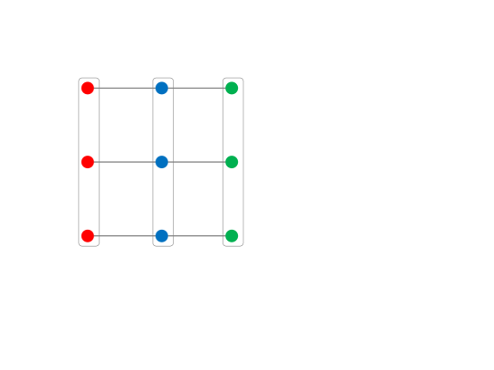
Figure 1: A $2$-dimensional hyperplane tessellated by the permutohedral lattice. The feature points are denoted with squares and the lattice points with circles. The neighborhood of the center lattice point is shaded and, for a feature point, the neighbouring lattice points are the vertices of the enclosing triangle.

Once the permutohedral lattice is constructed, the algorithm performs three main steps: splatting, blurring and slicing. During splatting, for each lattice point, the values of the neighbouring feature points are accumulated using barycentric interpolation. Next, during blurring, the values of the lattice points are convolved with a one dimensional truncated Gaussian kernel along each feature dimension separately. Finally, during slicing, the resulting values of the lattice points are propagated back to the feature points using the same barycentric weights. These steps are explained graphically in the top row of Fig. 2. The pseudocode of the algorithm is given in Appendix B.1. The time complexity of this algorithm is $\mathcal{O}(dn)$ [1, 12], and the complexity of the permutohedral lattice creation $\mathcal{O}(d^{2}n)$. Since the approach in [6] creates multiple lattices at every iteration, the overall complexity of this approach is $\mathcal{O}(d^{2}n\log(n))$.

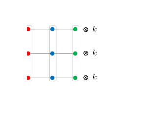
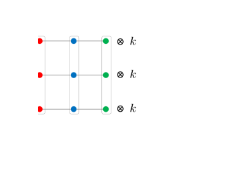
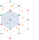
(a) Splat

(b) Blur

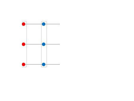
(c) Slice

Figure 2: Top row: Original filtering method. The barycentric interpolation is denoted by an arrow and $k$ here is the truncated Gaussian kernel. During splatting, for each lattice point, the values of the neighbouring feature points are accumulated using barycentric interpolation. Next, the lattice points are blurred with $k$ along each dimension. Finally, the values of the lattice points are given back to the feature points using the same barycentric weights. Bottom row: Our modified filtering method. Here, $H=3$, and the figure therefore illustrates 3 lattices. We write the bin number of each feature point next to the point. Note that, at the splatting step, the value of a feature point is accumulated to its neighbouring lattice points only if it is above or equal to the feature point level. Then, blurring is performed at each level independently. Finally, the resulting values are recovered from the lattice points at the feature point level.

Note that, in this original algorithm, there is no notion of score $y_{a}$ associated with each pixel. In particular, during splatting, the values $v_{a}$ are accumulated to the neighbouring lattice points without considering their scores. Therefore, this algorithm cannot be directly applied to handle our ordering constraint $\mathbbm{1}[y_{a}\geq y_{b}]$.

4.2 Modified filtering method

We now introduce a filtering-based algorithm that can handle ordering constraints. To this end, we uniformly discretize the continuous interval $[0,1]$ into $H$ different discrete bins, or levels. Note that each pixel, or feature point, belongs to exactly one of these bins, according to its corresponding score. We then propose to instantiate $H$ permutohedral lattices, one for each level $h\in\{0\ldots H-1\}$. In other words, at each level $h$, there is a lattice point $l$, whose value we denote by $\bar{v}_{l:h}$. To handle the ordering constraints, we then modify the splatting step in the following manner. A feature point belonging to bin $q$ is splat to the permutohedral lattices corresponding to levels $q\leq h<H$. Blurring is then performed independently in each individual permutohedral lattice. This guarantees that a feature point will only influence the values of the feature points that belong to the same level or higher ones. In other words, a feature point $b$ influences the value of a feature point $a$ only if $y_{a}\geq y_{b}$. Finally, during the slicing step, the value of a feature point belonging to level $q$ is recovered from the $q^{\rm th}$ permutohedral lattice. Our algorithm is depicted graphically in the bottom row of Fig. 2. Its pseudocode is provided in Appendix B.2. Note that, while discussed for constraints of the form $\mathbbm{1}[y_{a}\geq y_{b}]$, this algorithm can easily be adapted to handle $\mathbbm{1}[y_{a}\leq y_{b}]$ constraints, which are required for the second term in Eq. (19).

Overall, our modified filtering method has a time complexity of $\mathcal{O}(Hdn)$ and a space complexity of $\mathcal{O}(Hdn)$. Note that the complexity of the lattice creation is still $\mathcal{O}(d^{2}n)$ and can be reused for each of the $H$ instances. Moreover, as opposed to the method in [6], this operation is performed only once, during the initialization step. In practice, we were able to choose $H$ as small as 10, thus achieving a substantial speedup compared to the divide-and-conquer strategy of [6]. By discretizing the interval $[0,1]$, we add another level of approximation to the overall algorithm. However, this approximation can be eliminated by using a dynamic data structure, which we briefly explain in Appendix B.2.1.

5 Related work

We review the past work on three different aspects of our work in order to highlight our contributions.

Dense CRF.

The fully-connected CRF has become increasingly popular for semantic segmentation. It is particularly effective at preventing oversmoothing, thus providing better accuracy at the boundaries of objects. As a matter of fact, in a complementary direction, many methods have now proposed to combine dense CRFs with convolutional neural networks [5, 21, 27] to achieve state-of-the-art performance on segmentation benchmarks.

The main challenge that had previously prevented the use of dense CRFs is their computational cost at inference, which, naively, is $\mathcal{O}(n^{2})$ per iteration. In the case of Gaussian pairwise potential, the efficient filtering method of [1] proved to be key to the tractability of inference in the dense CRF. While an approximate method, the accuracy of the computation proved sufficient for practical purposes. This was first observed in [12] for the specific case of mean-field inference. More recently, several continuous relaxations, such as QP, DC and LP, were also shown to be applicable to minimizing the dense CRF energy by exploiting this filtering procedure in various ways [6]. Unfortunately, while tractable, minimizing the LP relaxation, which is known to provide the best approximation to the original labelling problem, remained too slow in practice [6]. Our algorithm is faster both theoretically and empirically. Furthermore, and as evidenced by our experiments, it yields lower energy values than any existing dense CRF inference strategy.

LP relaxation.

There are two ways to relax the integer program (3) to a linear program, depending on the label compatibility function: 1) the standard LP relaxation [4]; and 2) the LP relaxation specialized to the Potts model [9]. There are many notable works on minimizing the standard LP relaxation on sparse CRFs. This includes the algorithms that directly make use the dual of this LP [10, 11, 24] and those based on a proximal minimization framework [17, 20]. Unfortunately, all of the above algorithms exploit the sparsity of the problem, and they would yield an $\mathcal{O}(n^{2})$ cost per iteration in the fully-connected case. In this work, we focus on the Potts model based LP relaxation for dense CRFs and provide an algorithm whose iterations have time complexity $\mathcal{O}(n)$. Even though we focus on the Potts model, as pointed out in [6], this LP relaxation can be extended to general label compatibility functions using a hierarchical Potts model [14].

Frank-Wolfe.

The optimization problem of structural support vector machines (SVM) has a form similar to our proximal problem. The Frank-Wolfe algorithm [8] was shown to provide an effective and efficient solution to such a problem via block-coordinate optimization [16]. Several works have recently focused on improving the performance of this algorithm [18, 22] and extended its application domain [13]. Our work draws inspiration from this structural SVM literature, and makes use of the Frank-Wolfe algorithm to solve a subtask of our overall LP minimization method. Efficiency, however, could only be achieved thanks to our modification of the efficient filtering procedure to handle ordering constraints.

To the best of our knowledge, our approach constitutes the first LP minimization algorithm for dense CRFs to have linear time iterations. Our experiments demonstrate the importance of this result on both speed and labelling quality. Being fast, our algorithm can be incorporated in any end-to-end learning framework, such as [27]. We therefore believe that it will have a significant impact on future semantic segmentation results, and potentially in other application domains.

6 Experiments

In this section, we will first discuss two variants that further speedup our algorithm and some implementation details. We then turn to the empirical results.

6.1 Accelerated variants

Empirically we observed that, our algorithm can be accelerated by restricting the optimization procedure to affect only relevant subsets of labels and pixels. These subsets can be identified from an intermediate solution of PROX-LP. In particular, we remove the label $i$ from the optimization if $y_{a:i}<0.01$ for all pixels $a$. In other words, the score of a label $i$ is insignificant for all the pixels. We denote this version as PROX-LP_ℓ. Similarly, we optimize over a pixel only if it is uncertain in choosing a label. Here, a pixel $a$ is called uncertain if $\max_{i}y_{a:i}<0.95$. In other words, no label has a score higher than $0.95$. The intuition behind this strategy is that, after a few iterations of PROX-LP_ℓ, most of the pixels are labelled correctly, and we only need to fine tune the few remaining ones. In practice, we limit this restricted set to $10\%$ of the total number of pixels. We denote this accelerated algorithm as PROX-LP${}_{\text{acc}}$. As shown in our experiments, PROX-LP${}_{\text{acc}}$ yields a significant speedup at virtually no loss in the quality of the results.

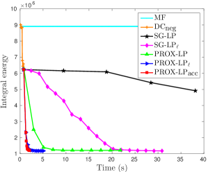
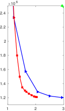
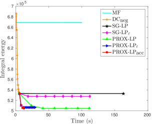
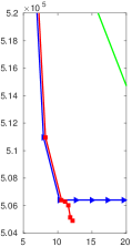
Figure 3: Assignment energy as a function of time for DC${}_{\text{neg}}$ parameters for an image in (left) MSRC and (right) Pascal. A zoomed-in version is shown next to each plot. Except MF, all other algorithms are initialized with DC${}_{\text{neg}}$. Note that PROX-LP clearly outperforms SG-LP_ℓ by obtaining much lower energies in fewer iterations. Furthermore, the accelerated versions of our algorithm obtain roughly the same energy as PROX-LP but significantly faster.

		MF5	MF	DC${}_{\text{neg}}$	SG-LPℓ	PROX-LP	PROX-LPℓ	PROX-LP${}_{\text{acc}}$	Ave. E ($\times 10^{3}$)	Ave. T (s)	Acc.	IoU
MSRC	MF5	-	0	0	0	0	0	0	8078.0	0.2	79.33	52.30
	MF	96	-	0	0	0	0	0	8062.4	0.5	79.35	52.32
	DC${}_{\text{neg}}$	96	96	-	0	0	0	0	3539.6	1.3	83.01	57.92
	SG-LPℓ	96	96	90	-	3	1	1	3335.6	13.6	83.15	58.09
	PROX-LP	96	96	94	92	-	13	45	1274.4	23.5	83.99	59.66
	PROX-LPℓ	96	96	95	94	81	-	61	1189.8	6.3	83.94	59.50
	PROX-LP${}_{\text{acc}}$	96	96	95	94	49	31	-	1340.0	3.7	84.16	59.65
Pascal	MF5	-	13	0	0	0	0	0	1220.8	0.8	79.13	27.53
	MF	2	-	0	0	0	0	0	1220.8	0.7	79.13	27.53
	DC${}_{\text{neg}}$	99	99	-	-	0	0	0	629.5	3.7	80.43	28.60
	SG-LPℓ	99	99	95	-	5	12	12	617.1	84.4	80.49	28.68
	PROX-LP	99	99	95	84	-	32	50	507.7	106.7	80.63	28.53
	PROX-LPℓ	99	99	86	86	64	-	43	502.1	22.1	80.65	28.29
	PROX-LP${}_{\text{acc}}$	99	99	86	86	46	39	-	507.7	14.7	80.58	28.45

Table 1: Results on the MSRC and Pascal datasets with the parameters tuned for DC${}_{\text{neg}}$. We show: the percentage of images where the row method strictly outperforms the column one on the final integral energy, the average integral energy over the test set, the average run time, the segmentation accuracy and the intersection over union score. Note that all versions of our algorithm obtain much lower energies than the baselines. Interestingly, while our fully accelerated version does slightly worse in terms of energy, it is the best in terms of the segmentation accuracy in MSRC.

6.2 Implementation details

In practice, we initialize our algorithm with the solution of the best continuous relaxation algorithm, which is called DC${}_{\text{neg}}$ in [6]. The parameters of our algorithm, such as the proximal regularization constant $\lambda$ and the stopping criteria, are chosen manually. A small value of $\lambda$ leads to easier minimization of the proximal problem, but also yields smaller steps at each proximal iteration. We found $\lambda=0.1$ to work well in all our experiments. We fixed the maximum number of proximal steps ($K$ in Algorithm 1) to 10, and each proximal step is optimized for a maximum of 5 Frank-Wolfe iterations ($T$ in Algorithm 1). In all our experiments the number of levels $H$ is fixed to $10$.

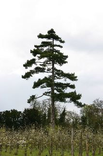
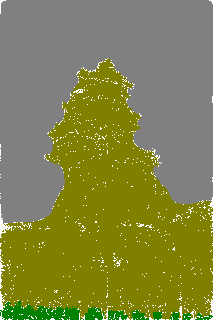
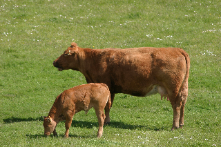
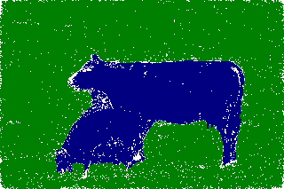
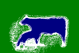
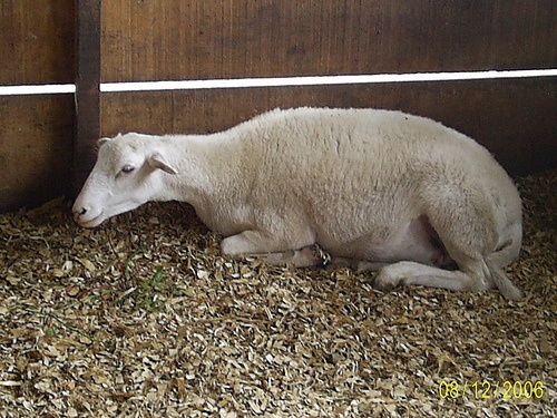
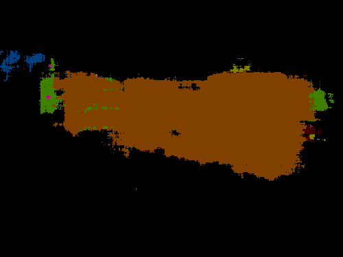
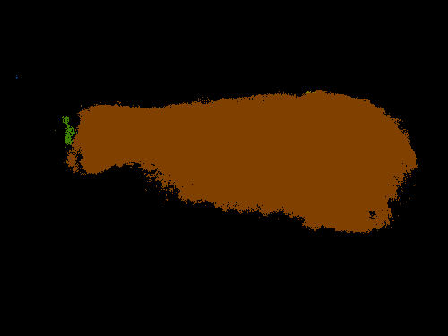
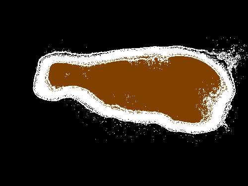
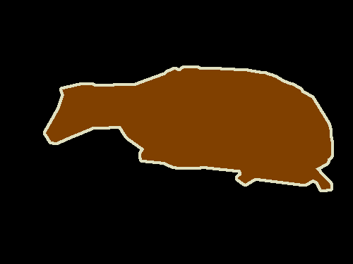
(a) Image

(b) MF

(c) DC${}_{\text{neg}}$

(d) SG-LP_ℓ

(e) PROX-LP

(f) PROX-LP_ℓ

(g) Uncer.(DC${}_{\text{neg}}$)

(h) Uncer.(ours)

(i) PROX-LP${}_{\text{acc}}$

(j) Ground truth

Figure 4: Results with DC${}_{\text{neg}}$ parameters, for an image in (top) MSRC and (bottom) Pascal. The uncertain pixels identified by DC${}_{\text{neg}}$ and PROX-LP${}_{\text{acc}}$ are marked in white. Note that, all versions of our algorithm obtain visually good segmentations. In addition, even though DC${}_{\text{neg}}$ is less accurate (the percentatge of uncertain pixels for DC${}_{\text{neg}}$ is usually less than 1%) in predicting uncertain pixels, our algorithm marks most of the crucial pixels (object boundaries and shadows) as uncertain. Furthermore, in the MSRC images, the improvement of PROX-LP${}_{\text{acc}}$ over the baselines is clearly visible and the final segmentation is virtually the same as the accurate ground truth. (Best viewed in color)

6.3 Segmentation results

We evaluated our algorithm on the MSRC and Pascal VOC 2010 [7] segmentation datasets, and compare it against mean-field inference (MF) [12], the best performing continuous relaxation method of [6] (DC${}_{\text{neg}}$) and the subgradient based LP minimization method of [6] (SG-LP). Note that, in [6], the LP was initialized with the DC${}_{\text{neg}}$ solution and optimized for 5 iterations. Furthermore, the LP optimization was performed on a subset of labels identified by the DC${}_{\text{neg}}$ solution in a similar manner to the one discussed in Section 6.1. We refer to this algorithm as SG-LP_ℓ. For all the baselines, we employed the respective authors’ implementations that were obtained from the web or through personal communication. Furthermore, for all the algorithms, the integral labelling is computed from the fractional solution using the argmax rounding scheme.

For both datasets, we used the same splits and unary potentials as in [12]. The pairwise potentials were defined using two kernels: a spatial kernel and a bilateral one [12]. For each method, the kernel parameters were cross validated on validation data using Spearmint [23]. To be able to compare energy values, we then evaluated all methods with the same parameters. In other words, for each dataset, each method was run several times with different parameter values. The final parameter values for MF and DC${}_{\text{neg}}$ are given in Appendix C.1. Note that, on MSRC, cross-validation was performed on the less accurate ground truth provided with the original dataset. Nevertheless, we evaluated all methods on the accurate ground truth annotations provided by [12].

The results for the parameters tuned for DC${}_{\text{neg}}$ on the MSRC and Pascal datasets are given in Table 1. Here MF5 denotes the mean-field algorithm run for 5 iterations. In Fig. 3, we show the assignment energy as a function of time for an image in MSRC (the tree image in Fig. 4) and for an image in Pascal (the sheep image in Fig. 4). Furthermore, we provide some of the segmentation results in Fig. 4.

In summary, PROX-LP_ℓ obtains the lowest integral energy in both datasets. Furthermore, our fully accelerated version is the fastest LP minimization algorithm and always outperforms the baselines by a great margin in terms of energy. From Fig. 4, we can see that PROX-LP${}_{\text{acc}}$ marks most of the crucial pixels (e.g., object boundaries) as uncertain, and optimizes over them efficiently and effectively. Note that, on top of being fast, PROX-LP${}_{\text{acc}}$ obtains the highest accuracy in MSRC for the parameters tuned for DC${}_{\text{neg}}$.

To ensure consistent behaviour across different energy parameters, we ran the same experiments for the parameters tuned for MF. In this setting, all versions of our algorithm again yield significantly lower energies than the baselines. The quantitative and qualitative results for this parameter setting are given in Appendix C.2.1.

6.4 Modified filtering method

We then compare our modified filtering method, described in Section 4, with the divide-and-conquer strategy of [6]. To this end, we evaluated both algorithms on one of the Pascal VOC test images (the sheep image in Fig. 4), but varying the image size, the number of labels and the Gaussian kernel standard deviation. Note that, to generate a plot for one variable, the other variables are fixed to their respective standard values. The standard value for the number of pixels is $187500$, for the number of labels $21$, and for the standard deviation $1$. For this experiment, the conditional gradients were computed from a random primal solution $\tilde{\mathbf{y}}^{t}$. In Fig. 5, we show the speedup of our modified filtering approach over the one of [6] as a function of the number of pixels and labels. As shown in Appendix C.4, the speedup with respect to the kernel standard deviation is roughly constant. The timings were averaged over 10 runs, and we observed only negligible timing variations between the different runs.

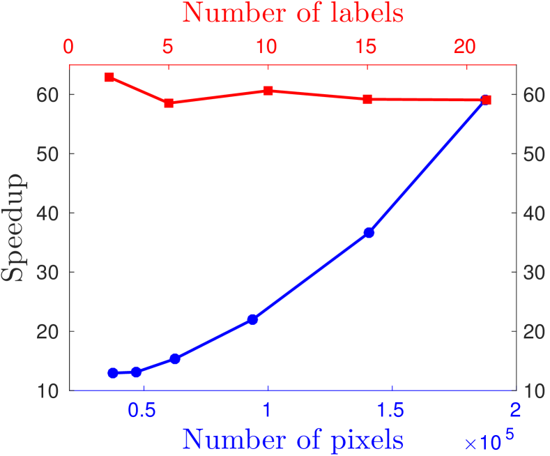
(a) Spatial kernel ($d=2$)

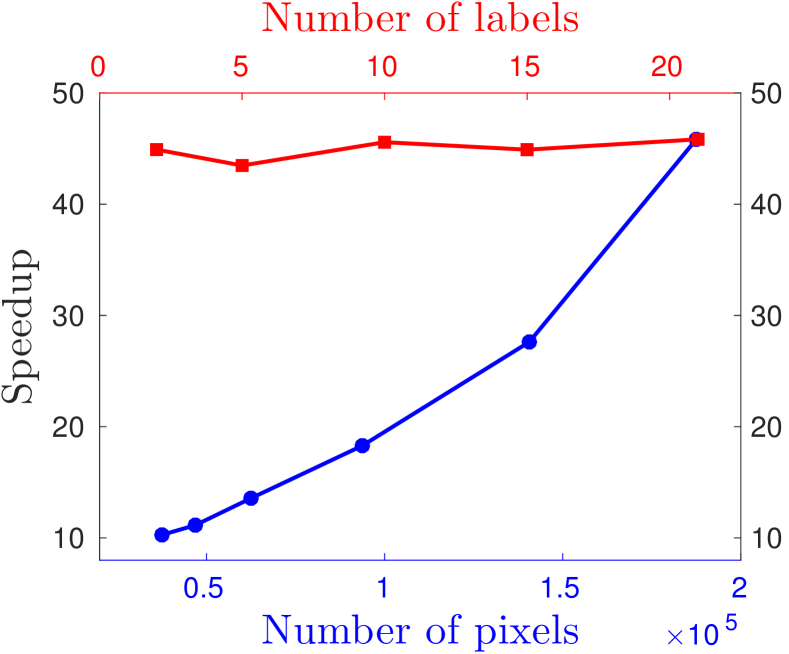
(b) Bilateral kernel ($d=5$)

Figure 5: Speedup of our modified filtering algorithm over the divide-and-conquer strategy of [6] on a Pascal image. Note that our speedup grows with the number of pixels and is approximately constant with respect to the number of labels. (Best viewed in color)

In summary, our modified filtering method is $10-65$ times faster than the state-of-the-art algorithm of [6]. Furthermore, note that all versions of our algorithm operate in the region where the speedup is around $45-65$.

7 Discussion

We have introduced the first LP minimization algorithm for dense CRFs with Gaussian pairwise potentials whose iterations are linear in the number of pixels and labels. Thanks to the efficiency of our algorithm and to the tightness of the LP relaxation, our approach yields much lower energy values than state-of-the-art dense CRF inference methods. Furthermore, our experiments demonstrated that, with the right set of energy parameters, highly accurate segmentation results can be obtained with our algorithm. The speed and effective energy minimization of our algorithm make it a perfect candidate to be incorporated in an end-to-end learning framework, such as [27]. This, we believe, will be key to further improving the accuracy of deep semantic segmentation architectures.

8 Acknowledgements

This work was supported by the EPSRC, the ERC grant ERC- 2012-AdG 321162-HELIOS, the EPSRC/MURI grant ref EP/N019474/1, the EPSRC grant EP/M013774/1, the EPSRC programme grant Seebibyte EP/M013774/1, the Microsoft Research PhD Scholarship, ANU PhD Scholarship and Data61 Scholarship. Data61 (formerly NICTA) is funded by the Australian Government as represented by the Department of Broadband, Communications and the Digital Economy and the Australian Research Council through the ICT Centre of Excellence program.

Appendix A Proximal minimization for LP relaxation - Supplementary material

In this section, we give the detailed derivation of our proximal minimization algorithm for the LP relaxation.

A.1 Dual formulation

Let us first restate the definition of the matrices $A$ and $B$, and analyze their properties. This would be useful to derive the dual of the proximal problem (9a).

Definition A.1.

Let $A\in\rm I\!R^{nm\times p}$ and $B\in\rm I\!R^{nm\times n}$ be two matrices such that

$$\left(A\boldsymbol{\alpha}\right)_{a:i} =-\sum_{b\neq a}\left(\alpha^{1}_{ab:i}-\alpha^{2}_{ab:i}+\alpha^{2}_{ba:i}-\alpha^{1}_{ba:i}\right)\ ,$$ (22)

$$\left(B\boldsymbol{\beta}\right)_{a:i} =\beta_{a}\ .$$

Proposition A.1.

Let $\mathbf{x}\in\rm I\!R^{nm}$. Then, for all $a\neq b$ and $i\in\mathcal{L}$,

$$\left(A^{T}\mathbf{x}\right)_{{ab:i}^{1}} =x_{b:i}-x_{a:i}\ ,$$ (23)

$$\left(A^{T}\mathbf{x}\right)_{{ab:i}^{2}} =x_{a:i}-x_{b:i}\ .$$

Here, the index ${{ab:i}^{1}}$ denotes the element corresponding to $\alpha^{1}_{ab:i}$.

Proof.

This can be easily proved by inspecting the matrix $A$. ∎

Proposition A.2.

The matrix $B\in\rm I\!R^{nm\times n}$ defined in Eq. (22) satisfies the following properties:

1. Let $\mathbf{x}\in\rm I\!R^{nm}$. Then, $\left(B^{T}\mathbf{x}\right)_{a}=\sum_{i\in\mathcal{L}}x_{a:i}$ for all $a\in\{1\ldots n\}$.

2. $B^{T}B=mI$, where $I\in\rm I\!R^{n\times n}$ is the identity matrix.

3. $BB^{T}$ is a block diagonal matrix, with each block $\left(BB^{T}\right)_{a}=\boldsymbol{1}$ for all $a\in\{1\ldots n\}$, where $\boldsymbol{1}\in\rm I\!R^{m\times m}$ is the matrix of all ones.

Proof.

Note that, from Eq. (22), the matrix $B$ simply repeats the elements $\beta_{a}$ for $m$ times. In particular, for $m=3$, the matrix $B$ has the following form:

$$B=\begin{bmatrix}1&0&\cdots&\cdots&\cdots&0\\[-5.69046pt] 1&\vdots&&&&\vdots\\[-5.69046pt] 1&0&\cdots&\cdots&\cdots&\vdots\\[-5.69046pt] 0&1&&&&\vdots\\[-5.69046pt] \vdots&1&&&&\vdots\\[-5.69046pt] \vdots&1&&&&\vdots\\[-5.69046pt] \vdots&0&&&&\vdots\\[-5.69046pt] \vdots&\vdots&&&&0\\[-5.69046pt] \vdots&\vdots&&&&1\\[-5.69046pt] \vdots&\vdots&&&&1\\ 0&\cdots&\cdots&\cdots&0&1\end{bmatrix}\ .$$ (24)

Therefore, multiplication by $B^{T}$ amounts to summing over the labels. From this, the other properties can be proved easily. ∎

We now derive the Lagrange dual of (9a).

Proposition A.3.

Given matrices $A\in\rm I\!R^{nm\times p}$ and $B\in\rm I\!R^{nm\times n}$ and dual variables $(\boldsymbol{\alpha},\boldsymbol{\beta},\boldsymbol{\gamma})$.

1. The Lagrange dual of (9a) takes the following form:

   $$\underset{\boldsymbol{\alpha},\boldsymbol{\beta},\boldsymbol{\gamma}}{\operatorname{min}}\ g(\boldsymbol{\alpha},\boldsymbol{\beta},\boldsymbol{\gamma}) =\frac{\lambda}{2}\|A\boldsymbol{\alpha}+B\boldsymbol{\beta}+\boldsymbol{\gamma}-\boldsymbol{\phi}\|^{2}+\left\langle A\boldsymbol{\alpha}+B\boldsymbol{\beta}+\boldsymbol{\gamma}-\boldsymbol{\phi},\mathbf{y}^{k}\right\rangle-\langle\boldsymbol{1},\boldsymbol{\beta}\rangle\ ,$$ (25)

   $$\text{s.t.}\hskip 34.69038pt\gamma_{a:i} \geq 0\quad\forall\,a\in\{1\ldots n\}\quad\forall\,i\in\mathcal{L}\ ,$$

   $$\hskip 34.69038pt\boldsymbol{\alpha}\in\mathcal{C} =\left\{\begin{array}[]{l|l}\hbox{\multirowsetup$\boldsymbol{\alpha}$}&\alpha^{1}_{ab:i}+\alpha^{2}_{ab:i}=\frac{K_{ab}}{2},\,\forall\,a\neq b,\,\forall\,i\in\mathcal{L}\\ &\alpha^{1}_{ab:i},\alpha^{2}_{ab:i}\geq 0,\,\forall\,a\neq b,\,\forall\,i\in\mathcal{L}\end{array}\right\}\ .$$ (28)

2. The primal variables $\mathbf{y}$ satisfy

   $$\mathbf{y}=\lambda\left(A\boldsymbol{\alpha}+B\boldsymbol{\beta}+\boldsymbol{\gamma}-\boldsymbol{\phi}\right)+\mathbf{y}^{k}\ .$$ (29)

Proof.

The Lagrangian associated with the primal problem (9a) can be written as [3]:

$$\underset{\boldsymbol{\alpha},\boldsymbol{\beta},\boldsymbol{\gamma}}{\operatorname{max}}\ \underset{\mathbf{y},\mathbf{z}}{\operatorname{min}}\ L(\boldsymbol{\alpha},\boldsymbol{\beta},\boldsymbol{\gamma},\mathbf{y},\mathbf{z}) =\sum_{a}\sum_{i}\phi_{a:i}\,y_{a:i}+\sum_{a,b\neq a}\sum_{i}\frac{K_{ab}}{2}z_{ab:i}+\frac{1}{2\lambda}\sum_{a}\sum_{i}\left(y_{a:i}-y^{k}_{a:i}\right)^{2}$$ (30)

$$+\sum_{a,b\neq a}\sum_{i}\alpha^{1}_{ab:i}\left(y_{a:i}-y_{b:i}-z_{ab:i}\right)+\sum_{a,b\neq a}\sum_{i}\alpha^{2}_{ab:i}\left(y_{b:i}-y_{a:i}-z_{ab:i}\right)$$

$$+\sum_{a}\beta_{a}\left(1-\sum_{i}y_{a:i}\right)-\sum_{a}\sum_{i}\gamma_{a:i}\,y_{a:i}\ ,$$

$$\text{s.t.}\hskip 43.36464pt\alpha^{1}_{ab:i},\alpha^{2}_{ab:i} \geq 0\quad\forall\,a\neq b\quad\forall\,i\in\mathcal{L}\ ,$$

$$\hskip 78.04842pt\gamma_{a:i} \geq 0\quad\forall\,a\in\{1\ldots n\}\quad\forall\,i\in\mathcal{L}\ .$$

Note that the dual problem is obtained by minimizing the Lagrangian over the primal variables $(\mathbf{y},\mathbf{z})$. With respect to $\mathbf{z}$, the Lagrangian is linear and when $\nabla_{\mathbf{z}}L(\boldsymbol{\alpha},\boldsymbol{\beta},\boldsymbol{\gamma},\mathbf{y},\mathbf{z})\neq 0$, the minimization in $\mathbf{z}$ yields $-\infty$. This situation is not useful as the dual function is unbounded. Therefore we restrict ourselves to the case where $\nabla_{\mathbf{z}}L(\boldsymbol{\alpha},\boldsymbol{\beta},\boldsymbol{\gamma},\mathbf{y},\mathbf{z})=0$. By differentiating with respect to $\mathbf{z}$ and setting the derivatives to zero, we obtain

$$\alpha^{1}_{ab:i}+\alpha^{2}_{ab:i}=\frac{K_{ab}}{2}\quad\forall\,a\neq b\quad\forall\,i\in\mathcal{L}\ .$$ (31)

The minimum of the Lagrangian with respect to $\mathbf{y}$ is attained when $\nabla_{\mathbf{y}}L(\boldsymbol{\alpha},\boldsymbol{\beta},\boldsymbol{\gamma},\mathbf{y},\mathbf{z})=0$. Before differentiating with respect to $\mathbf{y}$, let us rewrite the Lagrangian using Eq. (31) and reorder the terms:

$$L(\boldsymbol{\alpha},\boldsymbol{\beta},\boldsymbol{\gamma},\mathbf{y},\mathbf{z}) =\sum_{a}\sum_{i}(\phi_{a:i}-\beta_{a}-\gamma_{a:i})\,y_{a:i}+\frac{1}{2\lambda}\sum_{a}\sum_{i}\left(y_{a:i}-y^{k}_{a:i}\right)^{2}+\sum_{a,b\neq a}\sum_{i}\left(\alpha^{1}_{ab:i}-\alpha^{2}_{ab:i}\right)\,y_{a:i}$$ (32)

$$+\sum_{a,b\neq a}\sum_{i}\left(\alpha^{2}_{ba:i}-\alpha^{1}_{ba:i}\right)\,y_{a:i}+\sum_{a}\beta_{a}\ .$$

Now, by differentiating with respect to $\mathbf{y}$ and setting the derivatives to zero, we get

$$\frac{1}{\lambda}\left(y_{a:i}-y^{k}_{a:i}\right) =-\sum_{b\neq a}\left(\alpha^{1}_{ab:i}-\alpha^{2}_{ab:i}+\alpha^{2}_{ba:i}-\alpha^{1}_{ba:i}\right)+\beta_{a}+\gamma_{a:i}-\phi_{a:i}\quad\forall\,a\in\{1\ldots n\}\quad\forall\,i\in\mathcal{L}\ .$$ (33)

Using Eq. (22), the above equation can be written in vector form as

$$\frac{1}{\lambda}\left(\mathbf{y}-\mathbf{y}^{k}\right)=A\boldsymbol{\alpha}+B\boldsymbol{\beta}+\boldsymbol{\gamma}-\boldsymbol{\phi}\ .$$ (34)

This proves Eq. (29). Now, using Eqs. (31) and (34), the dual problem can be written as

$$\underset{\boldsymbol{\alpha},\boldsymbol{\beta},\boldsymbol{\gamma}}{\operatorname{min}}\ g(\boldsymbol{\alpha},\boldsymbol{\beta},\boldsymbol{\gamma}) =\frac{\lambda}{2}\|A\boldsymbol{\alpha}+B\boldsymbol{\beta}+\boldsymbol{\gamma}-\boldsymbol{\phi}\|^{2}+\left\langle A\boldsymbol{\alpha}+B\boldsymbol{\beta}+\boldsymbol{\gamma}-\boldsymbol{\phi},\mathbf{y}^{k}\right\rangle-\langle\boldsymbol{1},\boldsymbol{\beta}\rangle\ ,$$ (35)

$$\text{s.t.}\hskip 34.69038pt\gamma_{a:i} \geq 0\quad\forall\,a\in\{1\ldots n\}\quad\forall\,i\in\mathcal{L}\ ,$$

$$\hskip 34.69038pt\boldsymbol{\alpha}\in\mathcal{C} =\left\{\begin{array}[]{l|l}\hbox{\multirowsetup$\boldsymbol{\alpha}$}&\alpha^{1}_{ab:i}+\alpha^{2}_{ab:i}=\frac{K_{ab}}{2},\,\forall\,a\neq b,\,\forall\,i\in\mathcal{L}\\ &\alpha^{1}_{ab:i},\alpha^{2}_{ab:i}\geq 0,\,\forall\,a\neq b,\,\forall\,i\in\mathcal{L}\end{array}\right\}\ .$$ (38)

Here, $\boldsymbol{1}$ denotes the vector of all ones of appropriate dimension. Note that we converted our problem to a minimization one by changing the sign of all the terms. This proves Eq. (25). ∎

A.2 Optimizing over $\boldsymbol{\beta}$ and $\boldsymbol{\gamma}$

In this section, for a fixed value of $\boldsymbol{\alpha}^{t}$, we optimize over $\boldsymbol{\beta}$ and $\boldsymbol{\gamma}$.

Proposition A.4.

If $\nabla_{\boldsymbol{\beta}}g(\boldsymbol{\alpha}^{t},\boldsymbol{\beta},\boldsymbol{\gamma})=0$, then $\boldsymbol{\beta}$ satisfy

$$\boldsymbol{\beta}=B^{T}\left(A\boldsymbol{\alpha}^{t}+\boldsymbol{\gamma}-\boldsymbol{\phi}\right)/m\ .$$ (39)

Proof.

By differentiating the dual objective $g$ with respect to $\boldsymbol{\beta}$ and setting the derivatives to zero, we obtain the above equation. Note that, from Proposition A.2, $B^{T}\mathbf{y}^{k}=\boldsymbol{1}$ since $\mathbf{y}^{k}\in\mathcal{M}$ (defined in Eq. (4)), and $B^{T}B=mI$. Both these identities are used to simplify the above equation. ∎

Let us now define a matrix $D$ and analyze its properties. This will be useful to simplify the optimization over $\boldsymbol{\gamma}$.

Definition A.2.

Let $D\in\rm I\!R^{nm\times nm}$ be a matrix that satisfy

$$D=I-\frac{BB^{T}}{m}\ ,$$ (40)

where $B$ is defined in Eq. (22).

Proposition A.5.

The matrix $D$ satisfies the following properties:

1. $D$ is block diagonal, with each block matrix $D_{a}=I-\boldsymbol{1}/m$, where $I\in\rm I\!R^{m\times m}$ is the identity matrix and $\boldsymbol{1}\in\rm I\!R^{m\times m}$ is the matrix of all ones.

2. $D^{T}D=D\ .$

Proof.

From Proposition A.2, the matrix $BB^{T}$ is block diagonal with each block $\left(BB^{T}\right)_{a}=\boldsymbol{1}$. Therefore $D$ is block diagonal with each block matrix $D_{a}=I-\boldsymbol{1}/m$. Note that the block matrices $D_{a}$ are identical. The second property can be proved using simple matrix algebra. ∎

Now we turn to the optimization over $\boldsymbol{\gamma}$.

Proposition A.6.

The optimization over $\boldsymbol{\gamma}$ decomposes over pixels where for a pixel $a$, this QP has the form

$$\underset{\boldsymbol{\gamma}_{a}}{\operatorname{\min}}\quad \frac{1}{2}\boldsymbol{\gamma}^{T}_{a}Q\boldsymbol{\gamma}_{a}+\left\langle\boldsymbol{\gamma}_{a},Q\left((A\boldsymbol{\alpha}^{t})_{a}-\boldsymbol{\phi}_{a}\right)+\mathbf{y}^{k}_{a}\right\rangle\ ,$$ (41)

s.t. $$\boldsymbol{\gamma}_{a}\geq\boldsymbol{0}\ .$$

Here, $\boldsymbol{\gamma}_{a}$ denotes the vector $\{\gamma_{a:i}\mid i\in\mathcal{L}\}$ and $Q=\lambda\left(I-\boldsymbol{1}/m\right)\in\rm I\!R^{m\times m}$, with $I$ the identity matrix and $\boldsymbol{1}$ the matrix of all ones.

Proof.

By substituting $\boldsymbol{\beta}$ in the dual problem (25) with Eq. (39), the optimization problem over $\boldsymbol{\gamma}$ takes the following form:

$$\underset{\boldsymbol{\gamma}}{\operatorname{min}}\ g(\boldsymbol{\alpha}^{t},\boldsymbol{\gamma}) =\frac{\lambda}{2}\|D(A\boldsymbol{\alpha}^{t}+\boldsymbol{\gamma}-\boldsymbol{\phi})\|^{2}+\left\langle D(A\boldsymbol{\alpha}^{t}+\boldsymbol{\gamma}-\boldsymbol{\phi}),\mathbf{y}^{k}\right\rangle+\frac{1}{m}\left\langle\boldsymbol{1},A\boldsymbol{\alpha}^{t}+\boldsymbol{\gamma}-\boldsymbol{\phi}\right\rangle\ ,$$ (42)

$$\text{s.t.}\hskip 30.35657pt\boldsymbol{\gamma} \geq\boldsymbol{0}\ ,$$

where $D=I-\frac{BB^{T}}{m}$.

Note that, since $\mathbf{y}^{k}\in\mathcal{M}$, from Proposition A.2, $B^{T}\mathbf{y}^{k}=\boldsymbol{1}$. Using this fact, the identity $D^{T}D=D$, and by removing the constant terms, the optimization problem over $\boldsymbol{\gamma}$ can be simplified:

$$\underset{\boldsymbol{\gamma}}{\operatorname{min}}\ g(\boldsymbol{\alpha}^{t},\boldsymbol{\gamma}) =\frac{\lambda}{2}\boldsymbol{\gamma}^{T}D\boldsymbol{\gamma}+\langle\boldsymbol{\gamma},\lambda D(A\boldsymbol{\alpha}^{t}-\boldsymbol{\phi})+\mathbf{y}^{k}\rangle\ ,$$ (43)

$$\text{s.t.}\hskip 30.35657pt\boldsymbol{\gamma} \geq\boldsymbol{0}\ .$$

Furthermore, since $D$ is block diagonal from Proposition A.5, we obtain

$$\underset{\boldsymbol{\gamma}\geq\boldsymbol{0}}{\operatorname{min}}\ g(\boldsymbol{\alpha}^{t},\boldsymbol{\gamma})=\sum_{a}\underset{\boldsymbol{\gamma}_{a}\geq\boldsymbol{0}}{\operatorname{min}}\ \frac{\lambda}{2}\boldsymbol{\gamma}^{T}_{a}D_{a}\boldsymbol{\gamma}_{a}+\langle\boldsymbol{\gamma}_{a},\lambda D_{a}\left((A\boldsymbol{\alpha}^{t})_{a}-\boldsymbol{\phi}_{a}\right)+\mathbf{y}^{k}_{a}\rangle\ ,$$ (44)

where the notation $\boldsymbol{\gamma}_{a}$ denotes the vector $\{\gamma_{a:i}\mid i\in\mathcal{L}\}$. By substituting $Q=\lambda\,D_{a}$, the QP associated with each pixel $a$ can be written as

$$\underset{\boldsymbol{\gamma}_{a}\geq\boldsymbol{0}}{\operatorname{\min}}\quad \frac{1}{2}\boldsymbol{\gamma}^{T}_{a}Q\boldsymbol{\gamma}_{a}+\left\langle\boldsymbol{\gamma}_{a},Q\left((A\boldsymbol{\alpha}^{t})_{a}-\boldsymbol{\phi}_{a}\right)+\mathbf{y}^{k}_{a}\right\rangle\ .$$ (45)

∎

Each of these $m$ dimensional quadratic programs (QP) are optimized using the iterative algorithm of [26]. Before we give the update equation, let us first write our problem in the form used in [26]. For a given $a\in\{1\ldots n\}$, this yields

$$\underset{\boldsymbol{\gamma}_{a}\geq\boldsymbol{0}}{\operatorname{min}}\ \frac{1}{2}\boldsymbol{\gamma}_{a}^{T}Q\boldsymbol{\gamma}_{a}-\left\langle\boldsymbol{\gamma}_{a},\mathbf{h}_{a}\right\rangle\ ,$$ (46)

where

$$Q =\lambda\left(I-\frac{\boldsymbol{1}}{m}\right)\ ,$$ (47)

$$\mathbf{h}_{a} =-Q\left((A\boldsymbol{\alpha}^{t})_{a}-\boldsymbol{\phi}_{a}\right)-\mathbf{y}^{k}_{a}\ .$$

Hence, at each iteration, the element-wise update equation has the following form:

$$\gamma_{a:i}=\gamma_{a:i}\left[\frac{2\,(Q^{-}\boldsymbol{\gamma}_{a})_{i}+h^{+}_{a:i}+c}{(|Q|\boldsymbol{\gamma}_{a})_{i}+h^{-}_{a:i}+c}\right]\ ,$$ (48)

where $Q^{-}=\max(-Q,0)$, $|Q|=\text{abs}(Q)$, $h^{+}_{a:i}=\max(h_{a:i},0)$ and $h^{-}_{a:i}=\max(-h_{a:i},0)$ and $0<c\ll 1$. These $\max$ and abs operations are element-wise. We refer the interested reader to [26] for more detail on this update rule.

Note that, even though the matrix $Q$ has $m^{2}$ elements, the multiplication by $Q$ can be performed in $\mathcal{O}(m)$. In particular, the multiplication by $Q$ can be decoupled into a multiplication by the identity matrix and a matrix of all ones, both of which can be performed in linear time. Similar observations can be made for the matrices $Q^{-}$ and $|Q|$. Hence, the time complexity of the above update is $\mathcal{O}(m)$. Once the optimal $\boldsymbol{\gamma}$ for a given $\boldsymbol{\alpha}^{t}$ is computed, the corresponding optimal $\boldsymbol{\beta}$ is given by Eq. (39).

A.3 Conditional gradient computation

Proposition A.7.

The conditional gradient $\mathbf{s}$ satisfy

$$\left(A\mathbf{s}\right)_{a:i}=-\sum_{b}\left(K_{ab}\mathbbm{1}[\tilde{y}^{t}_{a:i}\geq\tilde{y}^{t}_{b:i}]-K_{ab}\mathbbm{1}[\tilde{y}^{t}_{a:i}\leq\tilde{y}^{t}_{b:i}]\right)\ ,$$ (49)

where $\tilde{\mathbf{y}}^{t}=\lambda\left(A\boldsymbol{\alpha}^{t}+B\boldsymbol{\beta}^{t}+\boldsymbol{\gamma}^{t}-\boldsymbol{\phi}\right)+\mathbf{y}^{k}$ using Eq. (29).

Proof.

The conditional gradient with respect to $\boldsymbol{\alpha}$ is obtained by solving the following linearization problem:

$$\mathbf{s}=\underset{\hat{\mathbf{s}}\in\mathcal{C}}{\operatorname{argmin}}\,\left\langle\hat{\mathbf{s}},\nabla_{\boldsymbol{\alpha}}g(\boldsymbol{\alpha}^{t},\boldsymbol{\beta}^{t},\boldsymbol{\gamma}^{t})\right\rangle\ ,$$ (50)

where

$$\nabla_{\boldsymbol{\alpha}}g(\boldsymbol{\alpha}^{t},\boldsymbol{\beta}^{t},\boldsymbol{\gamma}^{t})=A^{T}\tilde{\mathbf{y}}^{t}\ ,$$ (51)

with $\tilde{\mathbf{y}}^{t}=\lambda\left(A\boldsymbol{\alpha}^{t}+B\boldsymbol{\beta}^{t}+\boldsymbol{\gamma}^{t}-\boldsymbol{\phi}\right)+\mathbf{y}^{k}$ using Eq. (29).

Note that the feasible set $\mathcal{C}$ is separable, i.e., it can be written as $\mathcal{C}=\prod_{a,\,b\neq a,\,i\in\mathcal{L}}\,\mathcal{C}_{ab:i}$, with
$\mathcal{C}_{ab:i}=\left\{(\alpha^{1}_{ab:i},\alpha^{2}_{ab:i})\mid\alpha^{1}_{ab:i}+\alpha^{2}_{ab:i}=K_{ab}/2,\alpha^{1}_{ab:i},\alpha^{2}_{ab:i}\geq 0\right\}$. Therefore, the conditional gradient can be computed separately, corresponding to each set $\mathcal{C}_{ab:i}$. This yields

$$\underset{\hat{s}^{1}_{ab:i},\hat{s}^{2}_{ab:i}}{\operatorname{\min}}\quad \hat{s}^{1}_{ab:i}\nabla_{\alpha^{1}_{ab:i}}g(\boldsymbol{\alpha}^{t},\boldsymbol{\beta}^{t},\boldsymbol{\gamma}^{t})+\hat{s}^{2}_{ab:i}\nabla_{\alpha^{2}_{ab:i}}g(\boldsymbol{\alpha}^{t},\boldsymbol{\beta}^{t},\boldsymbol{\gamma}^{t})\ ,$$ (52)

s.t. $$\hat{s}^{1}_{ab:i}+\hat{s}^{2}_{ab:i}=K_{ab}/2\ ,$$

$$\hat{s}^{1}_{ab:i},\hat{s}^{2}_{ab:i}\geq 0\ ,$$

where, using Proposition A.1, the gradients can be written as:

$$\nabla_{\alpha^{1}_{ab:i}}g(\boldsymbol{\alpha}^{t},\boldsymbol{\beta}^{t},\boldsymbol{\gamma}^{t}) =\tilde{y}^{t}_{b:i}-\tilde{y}^{t}_{a:i}\ ,$$ (53)

$$\nabla_{\alpha^{2}_{ab:i}}g(\boldsymbol{\alpha}^{t},\boldsymbol{\beta}^{t},\boldsymbol{\gamma}^{t}) =\tilde{y}^{t}_{a:i}-\tilde{y}^{t}_{b:i}\ .$$

Hence, the minimum is attained at:

$$s^{1}_{ab:i} =\left\{\begin{array}[]{ll}K_{ab}/2&\mbox{if $\tilde{y}^{t}_{a:i}\geq\tilde{y}^{t}_{b:i}$}\\ 0&\mbox{otherwise}\ ,\end{array}\right.$$ (56)

$$s^{2}_{ab:i} =\left\{\begin{array}[]{ll}K_{ab}/2&\mbox{if $\tilde{y}^{t}_{a:i}\leq\tilde{y}^{t}_{b:i}$}\\ 0&\mbox{otherwise}\ .\end{array}\right.$$ (59)

Now, from Eq. (22), $A\mathbf{s}$ takes the following form:

$$\left(A\mathbf{s}\right)_{a:i} =-\sum_{b\neq a}\left(\frac{K_{ab}}{2}\mathbbm{1}[\tilde{y}^{t}_{a:i}\geq\tilde{y}^{t}_{b:i}]-\frac{K_{ab}}{2}\mathbbm{1}[\tilde{y}^{t}_{a:i}\leq\tilde{y}^{t}_{b:i}]+\frac{K_{ba}}{2}\mathbbm{1}[\tilde{y}^{t}_{b:i}\leq\tilde{y}^{t}_{a:i}]-\frac{K_{ba}}{2}\mathbbm{1}[\tilde{y}^{t}_{b:i}\geq\tilde{y}^{t}_{a:i}]\right)\ ,$$ (60)

$$=-\sum_{b}\left(K_{ab}\mathbbm{1}[\tilde{y}^{t}_{a:i}\geq\tilde{y}^{t}_{b:i}]-K_{ab}\mathbbm{1}[\tilde{y}^{t}_{a:i}\leq\tilde{y}^{t}_{b:i}]\right)\ .$$

Here, we used the symmetry of the kernel matrix $K$ to obtain this result. Note that the second equation is a summation over $b\in\{1\ldots n\}$. This is true due to the identity $K_{aa}\mathbbm{1}[\tilde{y}^{t}_{a:i}\geq\tilde{y}^{t}_{a:i}]-K_{aa}\mathbbm{1}[\tilde{y}^{t}_{a:i}\leq\tilde{y}^{t}_{a:i}]=0$ when $b=a$. ∎

A.4 Optimal step size

Proposition A.8.

The optimal step size $\delta$ satisfy

$$\delta=P_{[0,1]}\left(\frac{\langle A\boldsymbol{\alpha}^{t}-A\mathbf{s}^{t},\tilde{\mathbf{y}}^{t}\rangle}{\lambda\|A\boldsymbol{\alpha}^{t}-A\mathbf{s}^{t}\|^{2}}\right)\ .$$ (61)

Here, $P_{[0,1]}$ denotes the projection to the interval $[0,1]$, that is, clipping the value to lie in $[0,1]$.

Proof.

The optimal step size $\delta$ gives the maximum decrease in the objective function $g$ given the descent direction $\mathbf{s}^{t}$. This can be formulated as the following optimization problem:

$$\underset{\delta}{\operatorname{min}}\quad \frac{\lambda}{2}\left\|A\boldsymbol{\alpha}^{t}+\delta\left(A\mathbf{s}^{t}-A\boldsymbol{\alpha}^{t}\right)+B\boldsymbol{\beta}^{t}+\boldsymbol{\gamma}^{t}-\boldsymbol{\phi}\right\|^{2}+\left\langle A\boldsymbol{\alpha}^{t}+\delta\left(A\mathbf{s}^{t}-A\boldsymbol{\alpha}^{t}\right)+B\boldsymbol{\beta}^{t}+\boldsymbol{\gamma}^{t}-\boldsymbol{\phi}),\mathbf{y}^{k}\right\rangle-\left\langle\boldsymbol{1},\boldsymbol{\beta}\right\rangle\ ,$$ (62)

$$\text{s.t.}\quad\delta \in[0,1]\ .$$

Note that the above function is optimized over the scalar variable $\delta$ and the minimum is attained when the derivative is zero. Hence, setting the derivative to zero, we have

$$0 =\lambda\left\langle\delta\left(A\mathbf{s}^{t}-A\boldsymbol{\alpha}^{t}\right)+A\boldsymbol{\alpha}^{t}+B\boldsymbol{\beta}^{t}+\boldsymbol{\gamma}^{t}-\boldsymbol{\phi},A\mathbf{s}^{t}-A\boldsymbol{\alpha}^{t}\right\rangle+\left\langle\mathbf{y}^{k},A\mathbf{s}^{t}-A\boldsymbol{\alpha}^{t}\right\rangle\ ,$$ (63)

$$\delta =\frac{\langle A\boldsymbol{\alpha}^{t}-A\mathbf{s}^{t},\lambda\left(A\boldsymbol{\alpha}^{t}+B\boldsymbol{\beta}^{t}+\boldsymbol{\gamma}^{t}-\boldsymbol{\phi}\right)+\mathbf{y}^{k}\rangle}{\lambda\|A\boldsymbol{\alpha}^{t}-A\mathbf{s}^{t}\|^{2}}\ ,$$

$$\delta =\frac{\langle A\boldsymbol{\alpha}^{t}-A\mathbf{s}^{t},\tilde{\mathbf{y}}^{t}\rangle}{\lambda\|A\boldsymbol{\alpha}^{t}-A\mathbf{s}^{t}\|^{2}}\ .$$

In fact, if the optimal $\delta$ is out of the interval $[0,1]$, the value is simply truncated to be in $[0,1]$. ∎

Appendix B Fast conditional gradient computation - Supplementary material

In this section, we give the technical details of the original filtering algorithm and then our modified filtering algorithm. To this end, we consider the following computation

$$\forall\,a\in\{1\ldots n\},\quad v^{\prime}_{a}=\sum_{b}k(\mathbf{f}_{a},\mathbf{f}_{b})\,v_{b}\,\mathbbm{1}[y_{a}\geq y_{b}]\ ,$$ (64)

with $y_{a},y_{b}\in[0,1]$ for all $a,b\in\{1\ldots n\}$. Note that the above equation is the same as Eq. (14), except for the multiplication by the scalar $v_{b}$. In Section 4, the value $v_{b}$ was assumed to be 1, but here we consider the general case where $v_{b}\in\rm I\!R$.

B.1 Original filtering algorithm

Let us first introduce some notations below. We denote the set of lattice points of the original permutohedral lattice with $\mathcal{P}$ and the neighbouring feature points of lattice point $l$ by $N(l)$. This neighbourhood is shown in Fig. 1 in the main paper. Furthermore, we denote the neighbouring lattice points of a feature point $a$ by $\bar{N}(a)$. In addition, the barycentric weight between the lattice point $l$ and feature point $b$ is denoted with $w_{lb}$. Furthermore, the value at feature point $b$ is denoted by $v_{b}$ and the value at lattice point $l$ is denoted by $\bar{v}_{l}$. Finally, the set of feature point scores is denoted by $\mathcal{Y}=\{y_{b}\mid b\in\{1\ldots n\}\}$, their set of values is denoted by $\mathcal{V}=\{v_{b}\mid b\in\{1\ldots n\}\}$ and the set of lattice point values is denoted by $\bar{\mathcal{V}}=\{\bar{v}_{l}\mid l\in\mathcal{P}\}$. The pseudocode of the algorithm is given in Algorithm 2.

Algorithm 2 Original filtering algorithm [1]

Permutohedral lattice $\mathcal{P}$, set of feature point values $\mathcal{V}$

$\mathcal{V}^{\prime}\leftarrow\boldsymbol{0}\quad\bar{\mathcal{V}}\leftarrow\boldsymbol{0}\quad\bar{\mathcal{V}}^{\prime}\leftarrow\boldsymbol{0}$$\triangleright$ Initialization

for all $l\in\mathcal{P}$ do$\triangleright$ Splatting

     for all $b\in N(l)$ do

         $\bar{v}_{l}\leftarrow\bar{v}_{l}+w_{lb}\,v_{b}$      

$\bar{\mathcal{V}}^{\prime}\leftarrow k\otimes\bar{V}$ $\triangleright$ Blurring

for all $a\in\{1\ldots n\}$ do$\triangleright$ Slicing

     for all $l\in\bar{N}(a)$ do

         $v^{\prime}_{a}\leftarrow v^{\prime}_{a}+w_{la}\,\bar{v}^{\prime}_{l}$      

B.2 Modified filtering algorithm

As mentioned in the main paper, the interval $[0,1]$ is discretized into $H$ bins. Note that each bin $h\in\{0\ldots H-1\}$ is associated with an interval which is identified as: $\left[\frac{h}{H-1},\frac{h+1}{H-1}\right)$. Note that, the last bin (with bin id $H-1$) is associated with the interval $[1,\cdot)$. Since $y_{b}\leq 1$, this bin contains the feature points whose scores are exactly $1$. Given the score $y_{b}$ of the feature point $b$, its bin/level can be identified as

$$h_{b}=\left\lfloor y_{b}*(H-1)\right\rfloor\ ,$$ (65)

where $\lfloor\cdot\rfloor$ denotes the standard floor function.

Furthermore, during splatting, the values $v_{b}$ are accumulated to the neighbouring lattice point only if the lattice point is above or equal to the feature point level. We denote the value at lattice point $l$ at level $h$ by $\bar{v}_{l:h}$. Formally, the barycentric interpolation at lattice point $l$ at level $h$ can be written as

$$\bar{v}_{l:h}=\sum_{\begin{subarray}{c}b\in N(l)\\ h_{b}\leq h\end{subarray}}w_{lb}\,v_{b}\ .$$ (66)

Then, blurring is performed independently at each discrete level $h$. Finally, during slicing, the resulting values are interpolated at the feature point level. Our modified algorithm is given in Algorithm 3. In this algorithm, we denote the set of values corresponding to all the lattice points at level $h$ as $\bar{\mathcal{V}}_{h}=\{v_{l:h}\mid l\in\mathcal{P}\}$.

Algorithm 3 Modified filtering algorithm

Permutohedral lattice $\mathcal{P}$, set of feature point values $\mathcal{V}$, discrete levels $H$, set of scores $\mathcal{Y}$

$\mathcal{V}^{\prime}\leftarrow\boldsymbol{0}\quad\bar{\mathcal{V}}\leftarrow\boldsymbol{0}\quad\bar{\mathcal{V}}^{\prime}\leftarrow\boldsymbol{0}$$\triangleright$ Initialization

for all $l\in\mathcal{P}$ do$\triangleright$ Splatting

     for all $b\in N(l)$ do

         $h_{b}\leftarrow\left\lfloor y_{b}*(H-1)\right\rfloor$

         for all $h\in\{h_{b}\ldots H-1\}$ do$\triangleright$ Splat at the feature point level and above

              $\bar{v}_{l:h}\leftarrow\bar{v}_{l:h}+w_{lb}\,v_{b}$               

for all $h\in\{0\ldots H-1\}$ do $\bar{\mathcal{V}}^{\prime}_{h}\leftarrow k\otimes\bar{\mathcal{V}}_{h}$ $\triangleright$ Blurring at each level independently

for all $a\in\{1\ldots n\}$ do$\triangleright$ Slicing

     $h_{a}\leftarrow\left\lfloor y_{a}*(H-1)\right\rfloor$

     for all $l\in\bar{N}(a)$ do

         $v^{\prime}_{a}\leftarrow v^{\prime}_{a}+w_{la}\,\bar{v}^{\prime}_{l:h_{a}}$$\triangleright$ Slice at the feature point level      

Note that the above algorithm is given for the constraint $\mathbbm{1}[y_{a}\geq y_{b}]$ (Eq. (14)). However, it is fairly easy to modify it for the $\mathbbm{1}[y_{a}\leq y_{b}]$ constraint. In particular, one needs to change the interval identified by the bin $h$ to: $\left(\frac{h-1}{H-1},\frac{h}{H-1}\right]$. Using this fact, one can easily derive the splatting and slicing equations for the $\mathbbm{1}[y_{a}\leq y_{b}]$ constraint. The algorithm given above introduces an approximation to the gradient computation that depends on the number of discrete bins $H$. However, this approximation can be eliminated by using a dynamic data structure which we briefly explain in the next section.

B.2.1 Adaptive version of the modified filtering algorithm

Here, we briefly explain the adaptive version of our modified algorithm, which replaces the fixed discretization with a dynamic data structure. Effectively, discretization boils down to storing a vector of length $H$ at each lattice point. Instead of such a fixed-length vector, one can use a dynamic data structure that grows with the number of different scores encountered at each lattice point in the splatting and blurring steps. In the worst case, i.e., when all the neighbouring feature points have different scores, the maximum number of values to store at a lattice point is

$$H=\max_{l}|N^{2}(l)|\ ,$$ (67)

where $N^{2}(l)$ denotes the union of neighbourhoods of the lattice point $l$ and its neighbouring lattice points (the vertices of the shaded hexagon in Fig. 1 in the main paper). In our experiments, we observed that $|N^{2}(l)|$ is usually less than 100, with an average around 10. Empirically, however, we found this dynamic version to be slightly slower than the static one. We conjecture that this is due to the static version benefitting from better compiler optimization. Furthermore, both the versions obtained results with similar precesion and therefore we used the static one for all our experiments.

Appendix C Additional experiments

Let us first explain the pixel compatibility function used in the experiments. We then turn to additional experiments.

C.1 Pixel compatibility function used in the experiments

As mentioned in the main paper, our algorithm is applicable to any pixel compatibility function that is composed of a mixture of Gaussian kernels. In all our experiments, we used two kernels, namely spatial kernel and bilateral kernel, similar to [6, 12]. Our pixel compatibility function can be written as

$$K_{ab}=w^{(1)}\,\exp\left(-\frac{|\mathbf{p}_{a}-\mathbf{p}_{b}|^{2}}{\sigma_{1}}\right)+w^{(2)}\,\exp\left(-\frac{|\mathbf{p}_{a}-\mathbf{p}_{b}|^{2}}{\sigma_{2:s}}-\frac{|\mathbf{I}_{a}-\mathbf{I}_{b}|^{2}}{\sigma_{2:c}}\right)\ ,$$ (68)

where $\mathbf{p}_{a}$ denotes the $(x,y)$ position of pixel $a$ measured from top left and $\mathbf{I}_{a}$ denotes the $(r,g,b)$ values of pixel $a$. Note that there are $5$ learnable parameters: $w^{(1)},\sigma_{1},w^{(2)},\sigma_{2:s},\sigma_{2:c}$. These parameters are cross validated for different algorithms on each data set. The final cross validated parameters for MF and DC_neg are given in Table 2. To perform this cross-validation, we ran Spearmint for 2 days for each algorithm on both datasets. Note that, due to this time limitation, we were able to run approximately 1000 Spearmint iterations on MSRC but only 100 iterations on Pascal. This is due to bigger images and larger validation set on the Pascal dataset. Hence, it resulted in less accurate energy parameters.

Data set	Algorithm	$w^{(1)}$	$\sigma_{1}$	$w^{(2)}$	$\sigma_{2:s}$	$\sigma_{2:c}$
MSRC	MF	7.467846	1.000000	4.028773	35.865959	11.209644
	DC${}_{\text{neg}}$	2.247081	3.535267	1.699011	31.232626	7.949970
Pascal	MF	100.000000	1.000000	74.877398	50.000000	5.454272
	DC${}_{\text{neg}}$	0.500000	3.071772	0.960811	49.785678	1.000000

Table 2: Parameters tuned for MF and DC${}_{\text{neg}}$ on the MSRC and Pascal validation sets using Spearmint [23].

C.2 Additional segmentation results

In this section we provide additional segmentation results.

C.2.1 Results on parameters tuned for MF

The results for the parameters tuned for MF on the MSRC and Pascal datasets are given in Table 3. In Fig. 6, we show the assignment energy as a function of time for an image in MSRC (the tree image in Fig. 7) and for an image in Pascal (the sheep image in Fig. 7). Furthermore, we provide some of the segmentation results in Fig. 7.

Interestingly, for the parameters tuned for MF, even though our algorithm obtains much lower energies, MF yields the best segmentation accuracy. In fact, one can argue that the parameters tuned for MF do not model the segmentation problem accurately, but were tuned such that the inaccurate MF inference yields good results. Note that, in the Pascal dataset, when tuned for MF, the Gaussian mixture coefficients are very high (see Table 2). In such a setting, DC${}_{\text{neg}}$ ended up classifying all pixel in most images as background. In fact, SG-LP_ℓ was able to improve over DC${}_{\text{neg}}$ in only 1% of the images, whereas all our versions improved over DC${}_{\text{neg}}$ in roughly 25% of the images. Furthermore, our accelerated versions could not get any advantage over the standard version and resulted in similar run times. Note that, in most of the images, the uncertain pixels are in fact the entire image, as shown in Fig. 7.

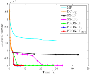
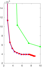
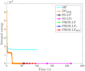
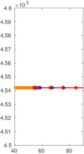
Figure 6: Assignment energy as a function of time for MF parameters for an image in (left) MSRC and (right) Pascal. A zoomed-in version is shown next to each plot. Except for MF, all the algorithms were initialized with DC${}_{\text{neg}}$. For the MSRC image, PROX-LP clearly outperforms SG-LP_ℓ by obtaining much lower energies in fewer iterations, and the accelerated versions of our algorithm obtain roughly the same energy as PROX-LP but significantly faster. For the Pascal image, however, no LP algorithm is able to improve over DC${}_{\text{neg}}$. Note that, in the Pascal dataset, for the MF parameters, DC${}_{\text{neg}}$ ended up classifying all pixel in most images as background (which yields low energy values) and no LP algorithm is able to improve over it.

		MF5	MF	DC${}_{\text{neg}}$	SG-LPℓ	PROX-LP	PROX-LPℓ	PROX-LP${}_{\text{acc}}$	Ave. E ($\times 10^{4}$)	Ave. T (s)	Acc.	IoU
MSRC	MF5	-	0	0	0	0	0	0	2366.6	0.2	81.14	54.60
	MF	95	-	18	15	2	1	2	1053.6	13.0	83.86	59.75
	DC${}_{\text{neg}}$	95	77	-	0	0	0	0	812.7	2.8	83.50	59.67
	SG-LPℓ	95	80	48	-	2	0	1	800.1	37.3	83.51	59.68
	PROX-LP	95	93	95	93	-	35	46	265.6	27.3	83.01	58.74
	PROX-LPℓ	95	94	94	94	59	-	43	261.2	13.9	82.98	58.62
	PROX-LP${}_{\text{acc}}$	95	93	93	93	49	46	-	295.9	7.9	83.03	58.97
Pascal	MF5	-	-	1	1	0	0	0	40779.8	0.8	80.42	28.66
	MF	93	-	3	3	0	0	1	20354.9	21.7	80.95	28.86
	DC${}_{\text{neg}}$	93	87	-	0	0	0	0	2476.2	39.1	77.77	14.93
	SG-LPℓ	93	87	1	-	0	0	0	2474.1	414.7	77.77	14.92
	PROX-LP	94	90	24	24	-	4	9	1475.6	81.0	78.04	15.79
	PROX-LPℓ	94	90	24	24	5	-	9	1458.9	82.7	78.04	15.79
	PROX-LP${}_{\text{acc}}$	94	89	28	27	18	18	-	1623.7	83.9	77.86	15.18

Table 3: Results on the MSRC and Pascal datasets with the parameters tuned for MF. We show: the percentage of images where the row method strictly outperforms the column one on the final integral energy, the average integral energy over the test set, the average run time, the segmentation accuracy and the intersection over union score. Note that all versions of our algorithm obtain much lower energies than the baselines. However, as expected, lower energy does not correspond to better segmentation accuracy, mainly due to the less accurate energy parameters. Furthermore, the accelerated versions of our algorithm are similar in run time and obtain similar energies compared to PROX-LP.

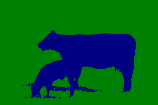
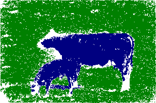
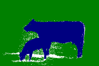
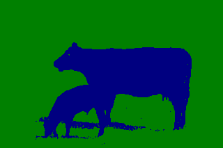
(a) Image

(b) MF

(c) DC${}_{\text{neg}}$

(d) SG-LP_ℓ

(e) PROX-LP

(f) PROX-LP_ℓ

(g) Uncer.(DC${}_{\text{neg}}$)

(h) Uncer.(ours)

(i) PROX-LP${}_{\text{acc}}$

(j) Ground truth

Figure 7: Results with MF parameters, for an image in (top) MSRC and (bottom) Pascal. The uncertain pixels identified by DC${}_{\text{neg}}$ and PROX-LP${}_{\text{acc}}$ are marked in white. Note that, in MSRC all versions of our algorithm obtain visually good segmentations similar to MF (or better). In Pascal, the segmentation results are poor except for MF, even though they obtain much lower energies. We argue that, in this case, the energy parameters do not model the segmentation problem accurately.

C.2.2 Summary

We have evaluated all the algorithms using two different parameter settings. Therefore, we summarize the best segmentation accuracy obtained by each algorithm and the corresponding parameter setting in Table 4. Note that, on MSRC, the best parameter setting for DC${}_{\text{neg}}$ corresponds to the parameters tuned for MF. This is a strange result but can be explained by the fact that, as mentioned in the main paper, cross-validation was performed using the less accurate ground truth provided with the original dataset, but evaluation using the accurate ground truth annotations provided by [12].

Furthermore, in contrast to MSRC, the segmentation results of our algorithm on the Pascal dataset is not the state-of-the-art, even with the parameters tuned for DC${}_{\text{neg}}$. This may be explained by the fact, that due to the limited cross-validation, the energy parameters obtained for the Pascal dataset is not accurate. Therefore, even though our algorithm obtained lower energies that was not reflected in the segmentation accuracy. Similar behaviour was observed in [6, 25].

Algorithm	MSRC			Pascal
	Parameters	Ave. T (s)	Acc.	Parameters	Ave. T (s)	Acc.
MF5	MF	0.2	81.14	MF	0.8	80.42
MF	MF	13.0	83.86	MF	21.7	80.95
DC${}_{\text{neg}}$	MF	2.8	83.50	DC${}_{\text{neg}}$	3.7	80.43
SG-LPℓ	MF	37.3	83.51	DC${}_{\text{neg}}$	84.4	80.49
PROX-LP	DC${}_{\text{neg}}$	23.5	83.99	DC${}_{\text{neg}}$	106.7	80.63
PROX-LPℓ	DC${}_{\text{neg}}$	6.3	83.94	DC${}_{\text{neg}}$	22.1	80.65
PROX-LP${}_{\text{acc}}$	DC${}_{\text{neg}}$	3.7	84.16	DC${}_{\text{neg}}$	14.7	80.58

Table 4: Best segmentation results of each algorithm with their respective parameters, the average time on the test set and the segmentation accuracy. In MSRC, the best segmentation accuracy is obtained by PROX-LP${}_{\text{acc}}$ and in Pascal it is by MF. Note that, on MSRC, the best parameter setting for DC${}_{\text{neg}}$ corresponds to the parameters tuned for MF. This is due to the fact that cross-validation was performed on the less accurate ground truth but evaluation on the accurate ground truth annotations provided by [12]. Furthermore, the low segmentation performance of our algorithm on the Pascal dataset is may be due to less accurate energy parameters resulted from limited cross-validation.

C.3 Effect of the proximal regularization constant

We plot the assignment energy as a function of time for an image in MSRC (the same image used to generate Fig. 3) by varying the proximal regularization constant $\lambda$. Here, we used the parameters tuned for DC${}_{\text{neg}}$. The plot is shown in Fig. 8. In summary, for a wide range of $\lambda$, PROX-LP obtains similar energies with approximately the same run time.

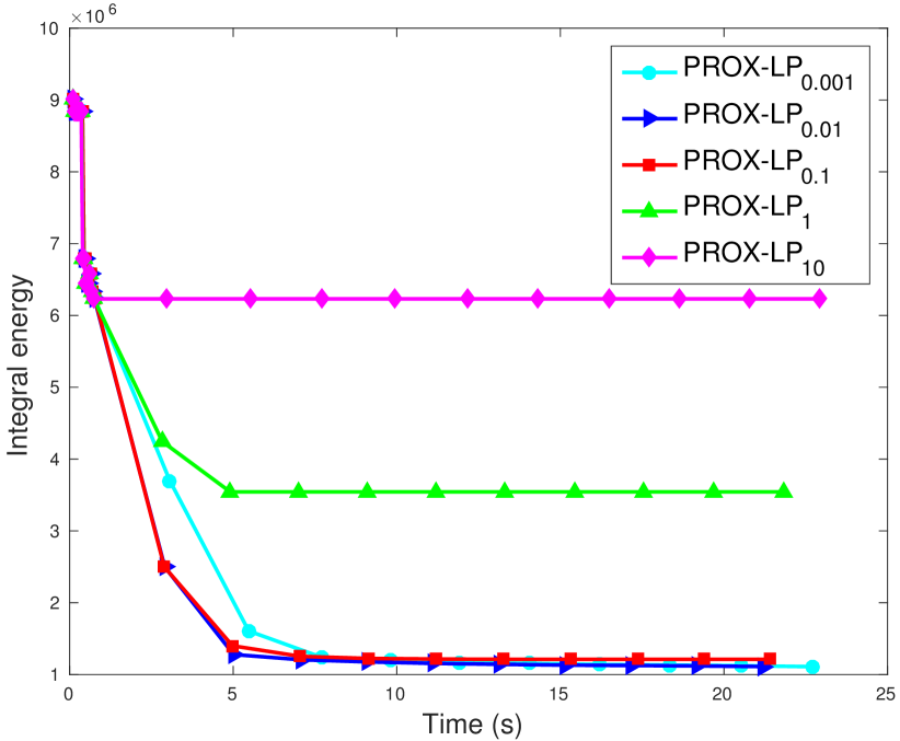
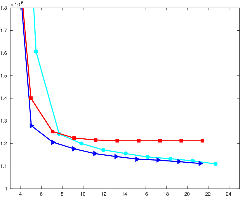
Figure 8: Assignment energy as a function of time for an image in MSRC, for different values of $\lambda$. The zoomed plot is shown on the right. Note that, for $\lambda=0.1,0.01,0.001$, PROX-LP obtains similar energies in approximately the same run time.

C.4 Modified filtering algorithm

We compare our modified filtering method, described in Section 4, with the divide-and-conquer strategy of [6]. To this end, we evaluated both algorithms on one of the Pascal VOC test images (the sheep image in Fig. 4), but varying the image size, the number of labels and the Gaussian kernel standard deviation. The respective plots are shown in Fig. 9. Note that, as claimed in the main paper, speedup with respect to the standard deviation is roughly constant. Similar plots for an MSRC image (the tree image in Fig. 4) are shown in Fig. 10. In this case, speedup is around $15-32$, with around $23-32$ in the operating region of all versions of our algorithm.

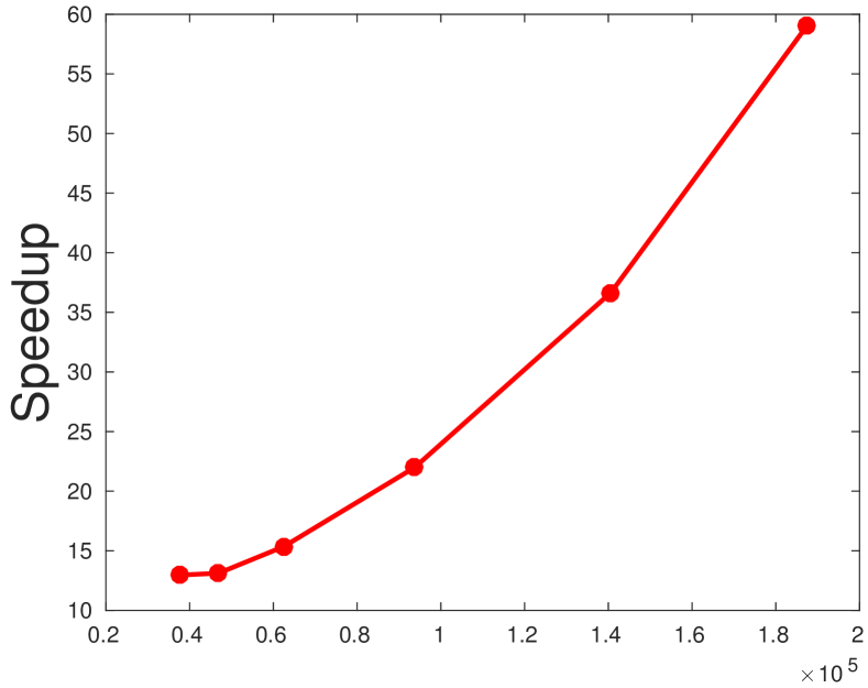
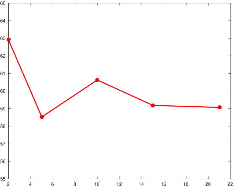
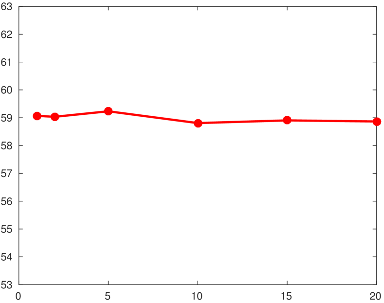
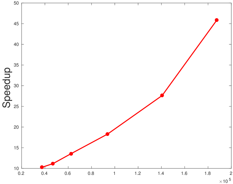
(a) Number of pixels

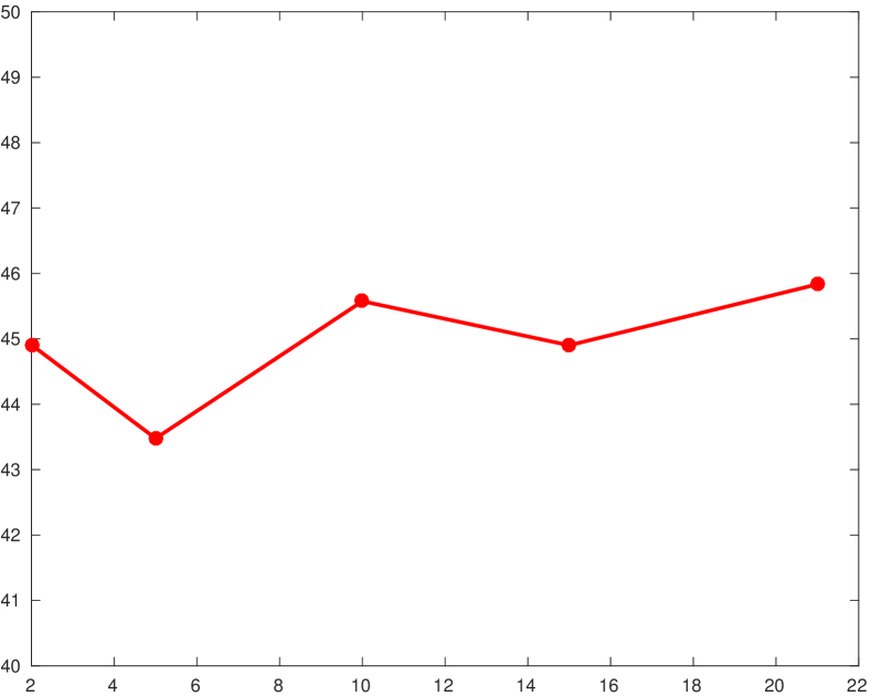
(b) Number of labels

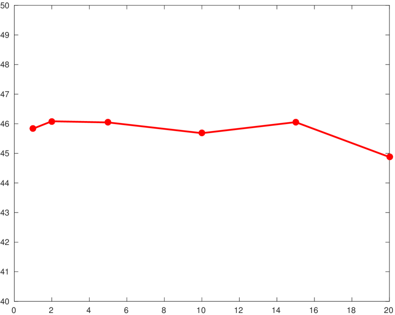
(c) Filter standard deviation

Figure 9: Speedup of our modified filtering algorithm over the divide-and-conquer strategy of [6] on a Pascal image, top: spatial kernel (d = 2), bottom: bilateral kernel (d = 5). Note that our speedup grows with the number of pixels and is approximately constant with respect to the number of labels and filter standard deviation.

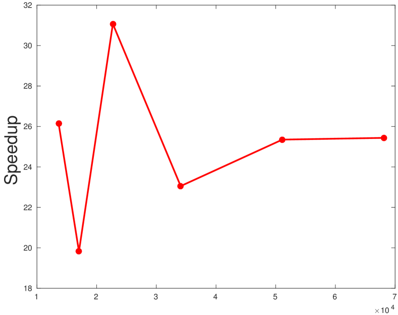
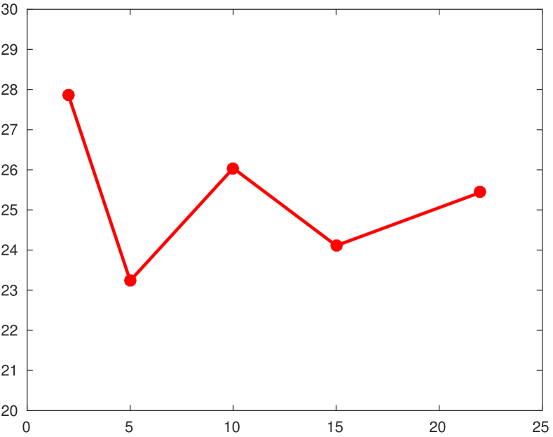
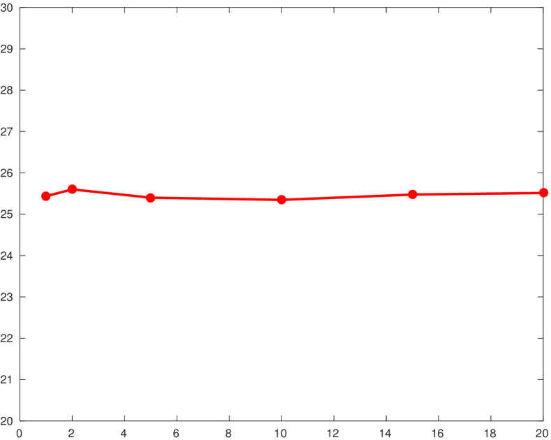
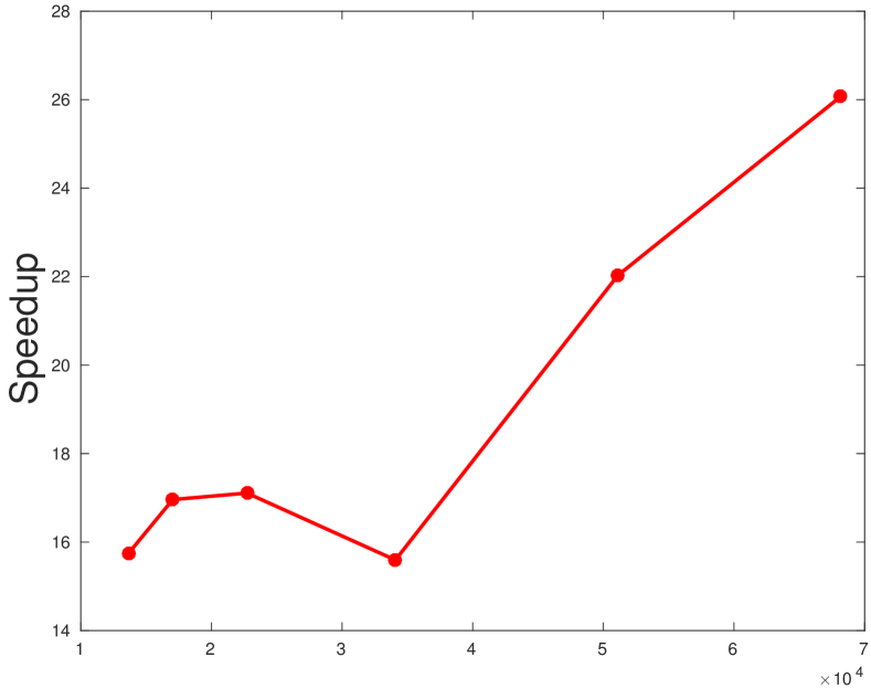
(a) Number of pixels

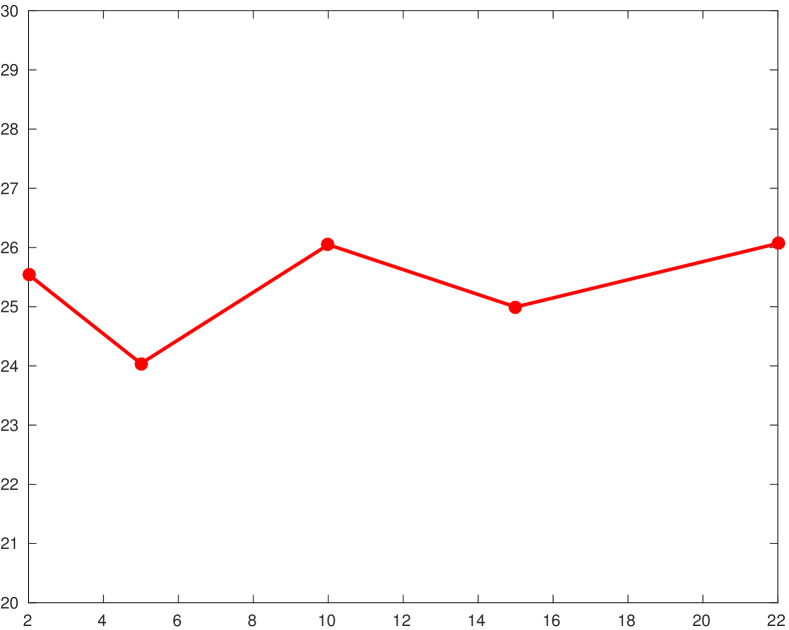
(b) Number of labels

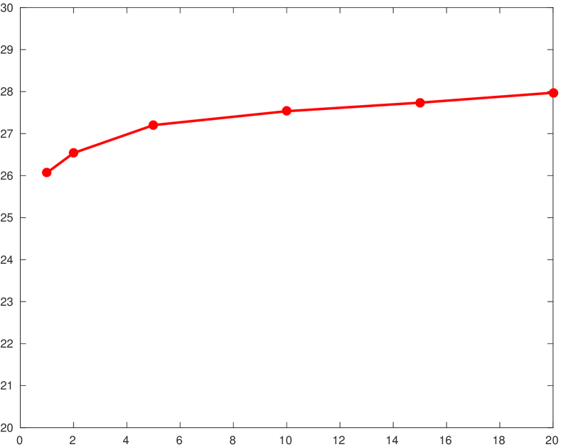
(c) Filter standard deviation

Figure 10: Speedup of our modified filtering algorithm over the divide-and-conquer strategy of [6] on a MSRC image, top: spatial kernel (d = 2), bottom: bilateral kernel (d = 5). Note that our speedup grows with the number of pixels and is approximately constant with respect to the number of labels and filter standard deviation.

References

- [1] A. Adams, J. Baek, and M. Davis. Fast high-dimensional filtering using the permutohedral lattice. In Computer Graphics Forum. Wiley Online Library, 2010.
- [2] F. Bach. Duality between subgradient and conditional gradient methods. SIAM Journal on Optimization, 2015.
- [3] S. Boyd and L. Vandenberghe. Convex optimization. Cambridge university press, 2009.
- [4] C. Chekuri, S. Khanna, J. Naor, and L. Zosin. A linear programming formulation and approximation algorithms for the metric labeling problem. SIAM Journal on Discrete Mathematics, 2004.
- [5] L. Chen, G. Papandreou, I. Kokkinos, K. Murphy, and A. Yuille. Semantic image segmentation with deep convolutional nets and fully connected CRFs. ICLR, 2014.
- [6] A. Desmaison, R. Bunel, P. Kohli, P. Torr, and P. Kumar. Efficient continuous relaxations for dense CRF. In ECCV. Springer, 2016.
- [7] M. Everingham, L. Van Gool, C. Williams, J. Winn, and A. Zisserman. The pascal visual object classes (VOC) challenge. IJCV, 2010.
- [8] M. Frank and P. Wolfe. An algorithm for quadratic programming. Naval research logistics quarterly, 1956.
- [9] J. Kleinberg and E. Tardos. Approximation algorithms for classification problems with pairwise relationships: metric labeling and markov random fields. Journal of the ACM, 2002.
- [10] V. Kolmogorov. Convergent tree-reweighted message passing for energy minimization. PAMI, 2006.
- [11] N. Komodakis, N. Paragios, and G. Tziritas. MRF energy minimization and beyond via dual decomposition. PAMI, 2011.
- [12] P. Krähenbühl and V. Koltun. Efficient inference in fully connected CRFs with gaussian edge potentials. NIPS, 2011.
- [13] R. Krishnan, S. Lacoste-Julien, and D. Sontag. Barrier Frank-Wolfe for marginal inference. NIPS, 2015.
- [14] P. Kumar and D. Koller. MAP estimation of semi-metric MRFs via hierarchical graph cuts. In UAI. AUAI Press, 2009.
- [15] P. Kumar, V. Kolmogorov, and P. Torr. An analysis of convex relaxations for MAP estimation of discrete MRFs. JMLR, 2009.
- [16] S. Lacoste-Julien, M. Jaggi, M. Schmidt, and P. Pletscher. Block-coordinate Frank-Wolfe optimization for structural SVMs. ICML, 2012.
- [17] O. Meshi, M. Mahdavi, and A. Schwing. Smooth and strong: MAP inference with linear convergence. In NIPS, 2015.
- [18] A. Osokin, J. Alayrac, I. Lukasewitz, P. Dokania, and S. Lacoste-Julien. Minding the gaps for block Frank-Wolfe optimization of structured SVMs. ICML, 2016.
- [19] N. Parikh and S. Boyd. Proximal algorithms. Foundations and Trends in Optimization, 2014.
- [20] P. Ravikumar, A. Agarwal, and M. Wainwright. Message-passing for graph-structured linear programs: proximal projections, convergence and rounding schemes. In ICML. ACM, 2008.
- [21] A. Schwing and R. Urtasun. Fully connected deep structured networks. CoRR, 2015.
- [22] N. Shah, V. Kolmogorov, and C. Lampert. A multi-plane block-coordinate Frank-Wolfe algorithm for training structural SVMs with a costly max-oracle. In CVPR, 2015.
- [23] J. Snoek, H. Larochelle, and R. Adams. Practical bayesian optimization of machine learning algorithms. In NIPS, 2012.
- [24] M. Wainwright, T. Jaakkola, and A. Willsky. MAP estimation via agreement on trees: message-passing and linear programming. Information Theory, 2005.
- [25] P. Wang, C. Shen, and A. van den Hengel. Efficient SDP inference for fully-connected CRFs based on low-rank decomposition. In CVPR, 2015.
- [26] X. Xiao and D. Chen. Multiplicative iteration for nonnegative quadratic programming. Numerical Linear Algebra with Applications, 2014.
- [27] S. Zheng, S. Jayasumana, B. Romera-Paredes, V. Vineet, Z. Su, D. Du, C. Huang, and P. Torr. Conditional random fields as recurrent neural networks. ICCV, 2015.