Structure of exciton condensates in imbalanced electron-hole bilayers

Abstract

We investigate the possibility of excitonic superfluidity in electron-hole bilayers. We calculate the phase diagram of the system for the whole range of electron-hole density imbalance and for different degrees of electrostatic screening, using mean-field theory and a Ginzburg-Landau expansion. We are able to resolve differences on previous work in the literature which concentrated on restricted regions of the parameter space. We also give detailed descriptions of the pairing wavefunction in the Fulde-Ferrell-Larkin-Ovchinnikov paired state. The Ginzburg-Landau treatment allows us to investigate the energy scales involved in the pairing state and discuss the possible spontaneous breaking of two-dimensional translation symmetry in the ground state.

I Introduction

Electron-hole systems have long been considered a candidate for fermionic superfluidity Blatt et al. (1962); Keldysh and Kozlov (1968); Nozières and Comte (1982); Moskalenko and Snoke (2000). The combination of the small effective masses of the electrons and holes and the long ranged nature of the Coulomb interaction between them should result in a higher critical temperature than atomic Fermi gases. By controlling the densities of electrons and holes, it should also be possible to tune the behavior of the condensed phase from a Bose-Einstein condensate of tightly bound excitons to a superfluid of weakly bound electron-hole pairs Nozières and Comte (1982). However, in bulk semiconductors, constant pumping is required to maintain the electron and hole populations as they are free to recombine. Any superfluidity will therefore be an inherently non-equilibrium phenomenon.

Bilayer quantum wells offer an alternative that can at least partially overcome this. These consist of two parallel quantum wells with an electric field applied perpendicular to the plane of the wells. This confines the electrons to one layer and holes to the other (Fig. 1). They may still recombine by tunneling, but the timescale over which this occurs is much longer than the thermalization time within each layer Lozovik and Yudson (1975). It may therefore be considered as an equilibrium system. Fermionic superfluidity and the BEC-BCS crossover should still be observable for sufficiently small interlayer spacing Lozovik and Yudson (1975); Littlewood and Zhu (1996); De Palo et al. (2002), but now with the excitons being formed by interlayer pairs.

Another possible realization can be achieved by coupling the electrons and holes in a bilayer quantum well to a single photon mode in an optical microcavity. Condensation of the coupled exciton-photon quasiparticles (exciton-polaritons) can then occur Eastham and Littlewood (2001); Deng et al. (2002); Szymanska et al. (2003); Kasprzak et al. (2006). These quasiparticles have a much smaller effective mass than the bare excitons, so have a correspondingly higher critical temperature. However, due to constant photon loss from the microcavity, they require constant pumping and the system is inherently out of equilibrium.

Recently, the ability to control the populations of electrons and holes in each layer independently has been developed for GaAs quantum wells Croxall et al. (2008); Seamons et al. (2009). Each of the two quantum wells in a GaAs-GaAlAs heterostructure is independently contacted with individual gate voltages so that the chemical potential in each layer can be tuned independently. This opens up the possibility of having mismatched electron and hole Fermi surfaces, allowing us to explore different types of ground states analogous to those predicted in spin-polarized superconductors and ultracold fermionic atomic systems.

Possible non-Fermi-liquid ground states include a superfluid of excitons (SF) formed by pairing electrons and holes with opposite in-plane momenta Nozières and Comte (1982). For weak binding, this is analogous to the Cooper pairs of BCS superconductors. For strong binding, this is analogous to the Bose-condensation limit in cold atomic Fermi gases. In bilayers with imbalanced hole and electron densities, it is also possible to pair up electrons and holes with unequal momenta. This is analogous to the Fulde-Ferrell-Larkin-Ovchinnikov (FFLO) states Fulde and Ferrell (1964); Larkin and Ovchinnikov (1965) for spin-polarized superconductors. Another candidate for imbalanced systems is the Sarma breached-pair state Sarma (1963) where a core region of the Fermi sphere form a BCS superfluid (with zero-momentum Cooper pairs) surrounded by unpaired quasiparticles of the majority carrier.

Early theoretical works examining this system have produced inconsistent and contradictory conclusions. Pieri et al. Pieri et al. (2007) and Subasi et al. Subası et al. (2010) calculated a mean-field phase diagram for the system in the canonical ensemble where the electron and hole populations in each layer are fixed. They found a rich phase diagram that included the BCS-type superfluid, and multiple variants of the Sarma phase. The possibility of an FFLO superfluid was also inferred from an instability in the free energy in the Sarma phase. However, since the bilayer electron and hole populations are controlled by a gate voltage, which controls the chemical potential in each layer and not the population directly, the experimentally relevant phase diagram should be calculated in the grand canonical ensemble.

The mean-field phase diagram for the grand canonical ensemble was calculated by Yamashita et al. Yamashita et al. (2010). It contained both BCS and FFLO superfluid regions, with a Sarma phase region only appearing at extreme electron-hole effective mass imbalances. Unfortunately, their phase diagram disagreed strongly with the results of Parish et al. Parish et al. (2011), which focussed on the limit of extreme population imbalance, with only one particle in one of the quantum well layers. In this limit, it was shown analytically that the system would always form a bound state for an unscreened interlayer Coulomb interaction, whereas the FFLO region phase diagram of Yamashita et al. did not extend all the way up to this fully imbalanced regime. In this work (Section IV), we span the whole phase diagram of the electron-hole bilayer and compare our results with these contradictory conclusions in the literature.

We will also address the issue of which FFLO states are favored in the ground state (Sections V and VI). The Fulde-Ferrell (FF) state has no density modulation while the Larkin-Ovchinnikov (LO) state has lines of nodes in space. Parish et al. Parish et al. (2011) showed that, in the limit of extreme imbalance, an electron-hole bilayer forms an excitonic condensate with two-dimensional spatial modulations in the order parameter. While that conclusion was based on a phenomenological theory of nonlinearities on the system, we provide a microscopic calculation of the nonlinearities in a Ginzburg-Landau theory. We find broad agreement with the phenomenological approach, and our calculation has extended the conclusion to the whole range of electron-hole imbalance. We also discovered key differences that give a different ground state. We are also able to provide an estimate for the energy scales for the FFLO condensation energy and the geometry of the two-dimensional state.

II The Model

In this paper, we study two parallel quantum wells with a two-dimensional electron layer in one well and a hole layer in the other well (Fig. 1). The single-particle energy at momentum $\hbar\mathbf{k}$ is given by

$$\xi_{\mathbf{k}\sigma}=\frac{\hbar^{2}\mathbf{k}^{2}}{2m_{\sigma}}-\mu-\sigma_{z}h$$ (1)

where $\sigma=h,e$ ($\sigma_{z}=\pm 1$) correspond to holes and electrons with effective masses $m_{h/e}$ respectively, $\mu$ is the mean chemical potential of the two layers and $h$ is the chemical potential imbalance (bias) between the layers. We assume that the separation $d$ of the wells is large enough that there is no tunneling between the layers.

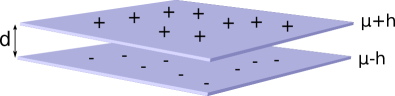
Figure 1: Schematic diagram of potentials of the electron-hole bilayer. The upper layer of holes has chemical potential $\mu_{h}=\mu+h$ while the lower layer of electrons has $\mu_{e}=\mu-h$.

The bare Coulomb interaction between an electron at the in-plane position $\mathbf{r}$ in one layer and at $\mathbf{r}^{\prime}$ in the other layer would be $-e^{2}/(|\mathbf{r}-\mathbf{r}^{\prime}|^{2}+d^{2})^{1/2}$. We work with a screened Coulomb interaction $V(\mathbf{r})$ in the Thomas-Fermi regime.

$$V(\mathbf{r})=\sum_{\mathbf{k}}V_{\mathbf{k}}e^{i\mathbf{k}\cdot\mathbf{r}}\,,\quad V_{\mathbf{k}}=\frac{2\pi e^{2}}{\epsilon_{r}A}\frac{e^{-|\mathbf{k}|d}}{|\mathbf{k}|+k_{\text{TF}}}$$ (2)

where $\mathbf{k}$ is the in-plane wavevector, $\epsilon_{r}$ is the relative permittivity and $A$ is the area of the system. This form is the static, long-wavelength limit of the screened interaction which can be obtained in a random phase approximation. Such a calculation gives a Thomas-Fermi screening wavevector $k_{\text{TF}}$ that is independent of the electron or hole densities but does depend on interlayer spacing. The Thomas-Fermi form is known to overestimate the effect of screening Świerkowski et al. (1995); Das Gupta et al. (2011); Neilson et al. (2014). Nevertheless, we retain this form of screening in this study, and use $k_{\text{TF}}$ as a parameter to control the strength of the electron-hole attractive interaction in this study. . Note that, in order to focus on the effect of interlayer attraction, we have also neglected intralayer interactions and are assuming that no non-Fermi-liquid correlations develop within each layer. (The consequence of intralayer repulsion can be mostly absorbed into a modified single-particle dispersion relation which adds algebraic complications to the calculation.)

The Hamiltonian of the system can be written as

$$H=\sum_{\sigma=e,h}\int\!\!d^{2}\mathbf{r}\,\,\,\psi^{\dagger}_{\sigma}(\mathbf{r})\xi_{\hat{\mathbf{k}}\sigma}\psi_{\sigma}(\mathbf{r})$$ (3)

$$-\iint\!\!d^{2}\mathbf{r}\,d^{2}\mathbf{r}^{\prime}\,\psi^{\dagger}_{h}(\mathbf{r})\psi^{\dagger}_{e}(\mathbf{r}^{\prime})V(\mathbf{r}-\mathbf{r}^{\prime})\psi_{e}(\mathbf{r}^{\prime})\psi_{h}(\mathbf{r})$$

where $\psi_{e}$ and $\psi_{h}$ are the electron and hole fields, respectively, and $\hat{\mathbf{k}}=-i\nabla$. Since we will be studying excitons in this system, we will from now on use the reduced mass of the exciton $m=(m_{e}^{-1}+m_{h}^{-1})^{-1}$ as the unit of mass, the exciton Bohr radius $a_{0}=\epsilon_{r}\hbar^{2}/me^{2}$ as the unit of length and the exciton Rydberg $R_{B}=e^{2}/\epsilon_{r}a_{0}$ as the unit of energy ($\sim$4.2 meV or equivalently $\sim$50K). It is also convenient to define the mass ratio $\alpha\equiv m_{h}/m_{e}$ and so $m_{h}=(1+\alpha)/2$ and $m_{e}=(1+\alpha)/2\alpha$. For this work, we present results for the symmetric case of $\alpha=1$ and also for $\alpha=4$ which is realistic for AlGaAs heterostructures.

III Mean-Field Theory for the exciton superfluid

In this section, we review the mean-field theory for excitonic condensation Yamashita et al. (2010). Consider the pairing of electrons at momentum $-\hbar(\mathbf{k}+\mathbf{Q}/2)$ with holes at momentum $\hbar(\mathbf{k}+\mathbf{Q}/2)$ to form excitons with a center-of-mass momentum of $\hbar\mathbf{Q}$. The case of $\mathbf{Q}=0$ is analogous to $s$-wave pairing in superconductors Nozières and Comte (1982). We will be label this as “SF”. There are different scenarios for condensation at non-zero $\mathbf{Q}$. Condensation at a single non-zero $\mathbf{Q}$ corresponds to the Fulde-Ferrell (FF) state discussed for spin-polarized superconductors Fulde and Ferrell (1964) and cold atomic gases Conduit et al. (2008). A state where excitons with momenta $\mathbf{Q}$ and $-\mathbf{Q}$ condense is the Larkin-Ovchinnikov (LO) state Larkin and Ovchinnikov (1965).

At high electron-hole population imbalance, there is no excitonic pairing. The ground state is a polarized state with separate electron and hole Fermi liquids in each layer. However, when the electron and hole populations are equal and their Fermi surfaces are identical, we expect excitonic pairing to occur to form excitons with zero total momentum for arbitrarily weak attractive interactions (as long as the density of states at the Fermi level is non-zero). So, we expect the onset of excitonic pairing at some non-zero bias $h$. The onset can be a transition directly into the $\mathbf{Q}=0$ exciton state (the Chandrasekhar-Clogston limit Chandrasekhar (1962); Clogston (1962)) or a FFLO phase with (single or multiple) non-zero $\mathbf{Q}$ can intervene at intermediate bias $h$. To map out the ground-state phases as a function of bias $h$ and the average chemical potential $\mu$, we first follow the standard mean-field treatment in deriving a gap equation for the excitonic order parameter which we will now outline to establish notation.

To investigate the pairing instability, we consider a simplified interaction involving only the interaction between electron-hole pairs with a discrete set of total momenta $\{\mathbf{Q}\}$:

$$V_{\text{int}}=-\sum_{\mathbf{k}\mathbf{k}^{\prime}\mathbf{Q}}V_{\mathbf{k}-\mathbf{k}^{\prime}}\psi^{\dagger}_{\mathbf{k}+\frac{\mathbf{Q}}{2}h}\psi^{\dagger}_{-\mathbf{k}+\frac{\mathbf{Q}}{2}e}\psi_{-\mathbf{k}^{\prime}+\frac{\mathbf{Q}}{2}e}\psi_{\mathbf{k}^{\prime}+\frac{\mathbf{Q}}{2}h}$$ (4)

where $\psi_{\mathbf{k}\sigma}=A^{-1/2}\int e^{-i\mathbf{k}\cdot\mathbf{r}}\psi_{\sigma}(\mathbf{r})\,d^{2}\mathbf{r}$ annihilates a particle with momentum $\hbar\mathbf{k}$. We introduce the static collective pairing field, $\Delta_{\mathbf{k}\mathbf{Q}}$, via a Hubbard-Stratonovich transformation, so that we obtain a pairing Hamiltonian

$$H_{\text{pair}} =F_{\Delta}+\sum_{\mathbf{k}\mathbf{Q}}\left(\Delta_{\mathbf{k}\mathbf{Q}}\,\psi^{\dagger}_{-\mathbf{k}+\frac{\mathbf{Q}}{2}h}\psi^{\dagger}_{\mathbf{k}+\frac{\mathbf{Q}}{2}e}+{\rm h.c.}\right)\,,$$

$$F_{\Delta} =\sum_{\mathbf{k}\mathbf{k}^{\prime}\mathbf{Q}}\overline{\Delta}_{\mathbf{k}\mathbf{Q}}V^{-1}_{\mathbf{k}\mathbf{k}^{\prime}}\Delta_{\mathbf{k}^{\prime}\mathbf{Q}}$$ (5)

where $V^{-1}_{\mathbf{k}\mathbf{k}^{\prime}}$ is the matrix inverse of $V_{\mathbf{k}-\mathbf{k}^{\prime}}$, regarding the latter as a matrix in its momentum labels $\mathbf{k}$ and $\mathbf{k}^{\prime}$. The mean-field value of the pairing field $\Delta_{\mathbf{k}\mathbf{Q}}$ is determined from the self-consistent equation:

$$\Delta_{{\mathbf{k}\mathbf{Q}}}=\sum_{\mathbf{k}^{\prime}}V_{\mathbf{k}-\mathbf{k}^{\prime}}\langle\psi_{-\mathbf{k}^{\prime}+\frac{\mathbf{Q}}{2}e}\psi_{\mathbf{k}^{\prime}+\frac{\mathbf{Q}}{2}h}\rangle$$ (6)

where the expectation value is taken with respect to the pairing Hamiltonian $H_{\text{pair}}$.

Let us now specialize to the Fulde-Ferrell state with a single exciton momentum $\mathbf{Q}$. It can be shown (see Appendix A) that the free energy of the mean-field Hamiltonian is given by:

$$F_{\text{MF}}=F_{\Delta}+\sum_{\mathbf{k}}(\xi^{+}_{{\mathbf{k}\mathbf{Q}}}-E_{{\mathbf{k}\mathbf{Q}}})-\frac{1}{\beta}\!\sum_{\genfrac{}{}{0.0pt}{2}{\mathbf{k}}{\alpha=\pm}}\!\ln(1+e^{-\beta{\cal E}_{\mathbf{k}\mathbf{Q}}^{\alpha}})$$ (7)

where $\beta=\hbar/k_{\rm B}T$ and $T$ is the temperature. The self-consistent equation is equivalent to minimizing $F_{\text{MF}}$ with respect to the pairing field (gap function) $\Delta_{\mathbf{k}\mathbf{Q}}$, leading to the ‘gap equation’:

$$\Delta_{\mathbf{k}\mathbf{Q}} =\sum_{\mathbf{k}^{\prime}}\frac{V_{\mathbf{k}-\mathbf{k}^{\prime}}\Delta_{{\mathbf{k}^{\prime}\mathbf{Q}}}}{2E_{{\mathbf{k}^{\prime}\mathbf{Q}}}}\left[1-f_{D}({\cal E}_{\mathbf{k}^{\prime}\mathbf{Q}}^{+})-f_{D}({\cal E}_{\mathbf{k}^{\prime}\mathbf{Q}}^{-})\right]\,,$$

$${\cal E}_{\mathbf{k}\mathbf{Q}}^{\pm} =E_{\mathbf{k}\mathbf{Q}}\pm\xi^{-}_{\mathbf{k}\mathbf{Q}}\,,\quad E_{\mathbf{k}}=\sqrt{(\xi^{+}_{\mathbf{k}\mathbf{Q}})^{2}+|\Delta_{\mathbf{k}\mathbf{Q}}|^{2}}$$ (8)

with $\xi^{\pm}_{\mathbf{k}\mathbf{Q}}=(\xi_{-\mathbf{k}+\frac{\mathbf{Q}}{2}h}\pm\xi_{\mathbf{k}+\frac{\mathbf{Q}}{2}e})/2$, and $f_{D}(E)=1/(e^{\beta E}+1)$ is the Fermi-Dirac distribution. The energies ${\cal E}_{\mathbf{k}\mathbf{Q}}^{\pm}$ correspond to the excitation energies of the fermionic quasiparticles of momentum $\hbar\mathbf{k}$ in the superfluid state.

The above gap equation gives the order parameter $\Delta_{{\mathbf{k}\mathbf{Q}}}$ as a function of $\mathbf{k}$ for a given exciton momentum $\hbar\mathbf{Q}$. It remains to find the wavevector $\mathbf{Q}$ that gives the lowest free energy. We will do this numerically when we discuss the phase diagram of the system.

From the free energy $F_{\text{MF}}$ (7) of the pairing Hamiltonian $H_{\text{pair}}$ (III), the total number density $n=n_{h}+n_{e}=-\partial F_{\text{MF}}/\partial\mu$ and imbalance $\delta n=n_{h}-n_{e}=-\partial F_{\text{MF}}/\partial h$ can be calculated.

$$\begin{split}n&=\frac{1}{A}\sum_{\mathbf{k}}\left\{1-\frac{\xi^{+}_{\mathbf{k}}}{E_{\mathbf{k}}}\left[1-f_{D}({\cal E}_{\mathbf{k}\mathbf{Q}}^{+})-f_{D}({\cal E}_{\mathbf{k}\mathbf{Q}}^{-})\right]\right\}\,,\\ \delta n&=\frac{1}{A}\sum_{\mathbf{k}}\left[f_{D}({\cal E}_{\mathbf{k}\mathbf{Q}}^{+})-f_{D}({\cal E}_{\mathbf{k}\mathbf{Q}}^{-})\right]\,.\end{split}$$ (9)

These will be used for converting from the grand canonical ensemble to the canonical ensemble in order to compare the results with those found in the work of Pieri et al. Pieri et al. (2007) and Tanatar et al. Subası et al. (2010).

From (9), we can immediately see that, if the quasiparticle energies ${\cal E}_{\mathbf{k}\mathbf{Q}}^{\pm}$ are both always greater than zero, there will be no population imbalance in the superfluid state. The superfluid will be of the BCS type. On the other hand, if any of the quasiparticle energies are negative, the population imbalance will be nonzero. Then, the superfluid will be of the Sarma type — a superfluid region in $\mathbf{k}$-space coexisting with regions of unpaired electrons and holes.

What about the mean-field theory for the Larkin-Ovchinnikov state where the exciton condensate has pairing at total momentum $\pm\hbar\mathbf{Q}$? The LO states involves spatial variation in the order parameter with wavevector $2\mathbf{Q}$. The eigenstates of the pairing Hamiltonian $H_{\text{pair}}$ form Bloch bands. As a result, the mean-field theory for the LO state (and other states with condensation into multiple momenta) is more complicated than the FF state and there are no general analytic results [see discussion at the end of Appendix A]. Nevertheless, as we explain in the section on a Ginzburg-Landau treatment for the onset of pairing, the FF and LO phases (and other phases involving condensation at wavevectors of the same magnitude) have the same ground-state energy in the limit of a vanishing order parameter. Thus, the analytic mean-field results for the SF ($\mathbf{Q}=0$) and FF phases are sufficient to locate the phase boundaries between the normal state and the SF or FFLO state, provided that it is a continuous (second-order) transition in the order parameter Larkin and Ovchinnikov (1965). We will see in the next section that this is indeed the case.

IV Phase Diagram

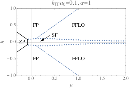
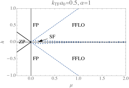
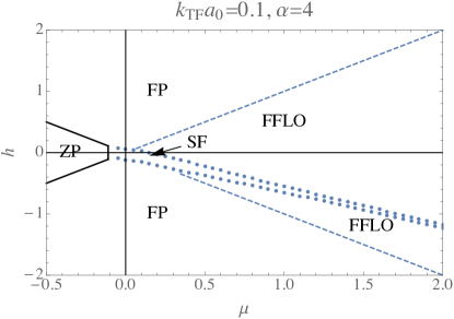
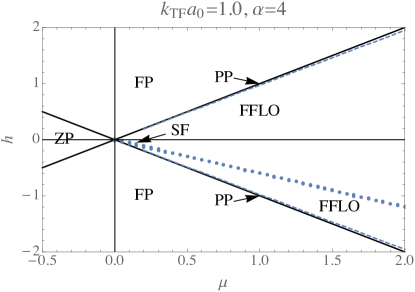
Figure 2: Ground states of the electron-hole bilayer as a function of chemical potential $\mu$ and bias $h$ at layer separation $d=a_{0}$. ZP: no particles, FP: fully polarized normal state with only electrons or only holes, PP: partially polarized normal state; SF: zero-momentum $\mathbf{Q}=0$ superfluid (SF), FFLO: exciton condensation at non-zero momenta ($\mathbf{Q}\neq 0$). Dotted line represents the SF-FFLO phase boundary (first-order transition). Dashed line represents FFLO-normal phase boundary (continuous transition). Left panel is for $\alpha=m_{h}/m_{e}=1$ with screening wavevectors $k_{\text{TF}}a_{0}=0.1$ and 0.5. There is a direct transition between FFLO phase and the fully polarized phase. Right panel is for $\alpha=4$ with $k_{\text{TF}}a_{0}=0.1$ and 1.0. The SF phase is centered around the line for which the normal state would have equal electron and hole populations. At small $k_{\text{TF}}a_{0}$, the FFLO phase extends all the way to the fully polarized (FP) limit. At higher $k_{\text{TF}}a_{0}$, a small region of PP normal state intervenes between the FFLO and FP states.

In this section, we discuss the ground states of the electron-hole bilayer as a function of the average chemical potential $\mu$ of the layers and the bias $h$ between the layers. We will compare our result for the grand canonical ensemble with results in the literature for the canonical ensemble. Also, we compare the difference between a Coulombic system and a system with contact interactions, appropriate for cold Fermi gases.

The ground states (Fig. 2) are identified using the gap equation (III) of the mean field theory from the previous section. The normal state is identified as the absence of a non-zero solution to the gap equation. For the superfluid states, we find numerically the ordering wavevector $\mathbf{Q}$ that minimizes the mean-field free energy $F_{\text{MF}}$. This allows us to distinguish between the BCS-like superfluid (SF) with electron-hole pairs with zero total momentum and the FFLO state where the electron-hole pair has non-zero momentum.

As mentioned in the previous section, the mean-field theory is sufficient to identify the boundary for a continuous transition of the normal state between an excitonic state. However, it does not guarantee that we have the correct boundary between the SF and FFLO phases because the order parameter $\Delta_{\mathbf{k}\mathbf{Q}}$ has a non-zero value at the phase boundary. (In fact, we find a discontinuous transition between the SF and FFLO phases, shown as dotted lines in Fig. 2.) In other words, the critical bias for the breakdown of the SF state will be different for different types of FFLO states. The boundary calculated here is only valid for the FF type with a single ordering wavevector $\mathbf{Q}$. Other FFLO structures may extend the boundary further into the superfluid region. For instance, in superconductors, the FFLO state near the FFLO-SF boundary can consist of a series of domain walls across which the order parameter changes sign Machida and Nakanishi (1984); Matsuo et al. (1998). Therefore, the value of $h_{c1}$ shown here only gives a ‘worst case’ scenario for the FFLO phase. It is possible that the FFLO phase penetrates into the SF region more deeply.

First of all, we note that we do not find a stable Sarma state in this region of parameters we explored. This is in contrast to previous work Pieri et al. (2007); Subası et al. (2010) at fixed electron and hole densities. As pointed out by Forbes et al. (2005) and Lamacraft and Marchetti (2008) (in the context of spin-imbalanced Fermi gases), the Sarma mean-field solution Sarma (1963) at fixed density is a local maximum in the free energy and physically represents an instability to spinodal decomposition. Moreover, those works Pieri et al. (2007); Subası et al. (2010) did not allow for finite values of the ordering wavevector in the FFLO and they miss the possibility of the FFLO phase coming from the normal side of the transition.

Let us consider now the SF phase which has a non-zero gap function $\Delta_{\mathbf{k},\mathbf{Q}=0}$. In the $\mu$-$h$ phase diagram (Fig. 2), this phase occupies a narrow region around the line $h/\mu=-(\alpha-1)/(\alpha+1)$ where $\alpha=m_{h}/m_{e}$ is the carrier mass ratio. This line is the line of equal electron and hole populations for the non-interacting (normal) system and hence equal Fermi surfaces. This SF region in the phase diagram become narrower at higher chemical potentials. To understand this, we note from Eq. (4) that the pairing of $\pm\mathbf{k}$ carriers require the interaction potential $V_{\mathbf{k}-\mathbf{k}^{\prime}}$ at $|\mathbf{k}-\mathbf{k}^{\prime}|=2k_{\text{F}}$. Since the Fermi surfaces are larger at higher $\mu$ and $V_{\mathbf{k}}$ decreases with $|\mathbf{k}|$ for our interaction (2), we see that the pairing instability is weakened at higher densities. This is in contrast with the case of contact interactions Conduit et al. (2008) with a constant $V_{\mathbf{k}}$ where the critical bias for the SF-FFLO boundary increases with chemical potential. A similar dependence on density, due to the interaction range as an additional lengthscale, has been seen in the BCS-BEC crossover for attractive fermionic gases Andrenacci et al. (1999); Parish et al. (2005).

As we increase $h$ away from the equal-population line, the SF pairing becomes less favorable owing to the mismatch in the sizes of the Fermi surfaces for the two carriers. The system can either transition directly to a normal state (Chandrasekhar-Clogston limit) or choose to form an exciton with finite momentum $\hbar\mathbf{Q}$. The latter case is the generic situation. The exception occurs at low $\mu$ and small $k_{\text{TF}}$ (top left in Fig. 2) where the critical bias occurs when $|h|>\mu$ so that the normal state is fully polarized, i.e. one of the layers is empty of carriers. Nevertheless, although a direct SF-normal transition is rare, the SF-FFLO boundary occurs at only a slightly lower field than predicted by the critical bias for the first-order Chandrasekhar-Clogston transition.

At sufficiently high bias $h$, the FFLO phase eventually gives way to a normal phase. For the case of equal mass ($\alpha=1$), we find that the FFLO phase is robust until $h=\mu$ when the system is fully polarized. In other words, FFLO pairing occurs for arbitrarily small minority carrier density. We are in agreement with Parish et al. Parish et al. (2011) but disagree with Yamashita et al. Yamashita et al. (2010) who see a large partially polarized region for the unscreened case ($\alpha\simeq 4$, $d=a_{0}$) with a large hole Fermi surface and a small electron Fermi surface. We searched for this partially polarized normal state. We found that such a state may be stable over a narrow range of bias close to the fully polarized state and only when there is significant screening ($k_{\text{TF}}a_{0}\sim 1$). This is illustrated in Fig. 2 for the mass ratio of $\alpha=4$. Note that the existence of a partially polarized state at strong screening is consistent with the observation that the FFLO phase is less robust for contact interactions where a wide region of the partially polarized phase exists in the phase diagram, as shown by Conduit et al. Conduit et al. (2008).

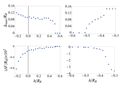
Figure 3: Continuous transition between Normal and FFLO state at $h=0.5$ (left) and $h=-0.5$ (right). Top panels show maximum value of the gap function $\Delta_{\textrm{max}}$ as a function of bias $h$ at $\mu=0.5$ and $k_{\text{TF}}a_{0}=0.1$ ($m_{h}/m_{e}=4$). Bottom panels show energy difference $\delta F$ between the SF or FF phase and the normal state.

To demonstrate that the normal-FF boundary is a continuous transition, we can examine the maximum value $\Delta_{\textrm{max}}$ of the gap function $\Delta_{\mathbf{k}\mathbf{Q}}$ as function of bias $h$ at a particular chemical potential $\mu=0.5$ (Fig. 3). In the superfluid phase (near $h=-0.3$), the order parameter does not vary with $h$, so its maximum is constant. In the FF phase, $\Delta_{\textrm{max}}$ decreases as $h$ is moved away from the equal population value, eventually going continuously to zero at the FFLO-Normal phase boundary ($h=\pm 0.5$).

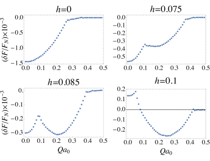
Figure 4: Free-energy difference $\delta F$ between FF state with wavevector $Q$ and normal state (of energy $F_{N}$) at $\mu=0.5$ at different values of the bias $h$. ($m_{h}/m_{e}=1,k_{\text{TF}}a_{0}=0.1$. The SF-FF transition occurs at $h=0.085$.

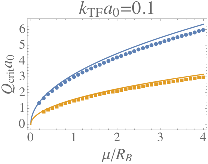
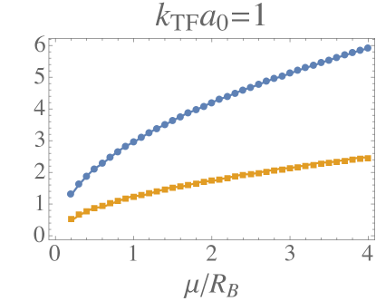
Figure 5: The ordering wavevectors (points) of the FF state at the two FFLO-normal phase boundaries ($\alpha=m_{h}/m_{e}=4$) as a function of chemical potential. $k_{\text{TF}}a_{0}$ = 0.1 (left), 1 (right). Solid line shows the naive estimate $|k_{\text{F}h}-k_{\text{F}e}|a_{0}$.

To demonstrate that the SF-FF transition is discontinuous, we can examine the free energy difference between the SF and FF states as a function of the ordering wavevector $\mathbf{Q}$ (Fig. 4). At equal population, the difference in energy has a single minimum at $Q=0$, corresponding to a gap function $\Delta_{\mathbf{k}\mathbf{Q}}$ that is isotropic in $\mathbf{k}$. As $h$ is increased a second minimum develops at a finite $Q$ with a pairing function that is anisotropic in $\mathbf{k}$. This is initially higher in energy than the $Q=0$ superfluid state. However, when $h$ is increased further, this $Q\neq 0$ minimum eventually becomes lower that the SF state, indicating a first-order phase transition. This implies phase separation for systems at fixed densities, which can be seen more clearly in a plot of the phase diagram in density space (see later, Fig. 7). (Note that such an instability may be prevented by long-ranged intralayer repulsion.)

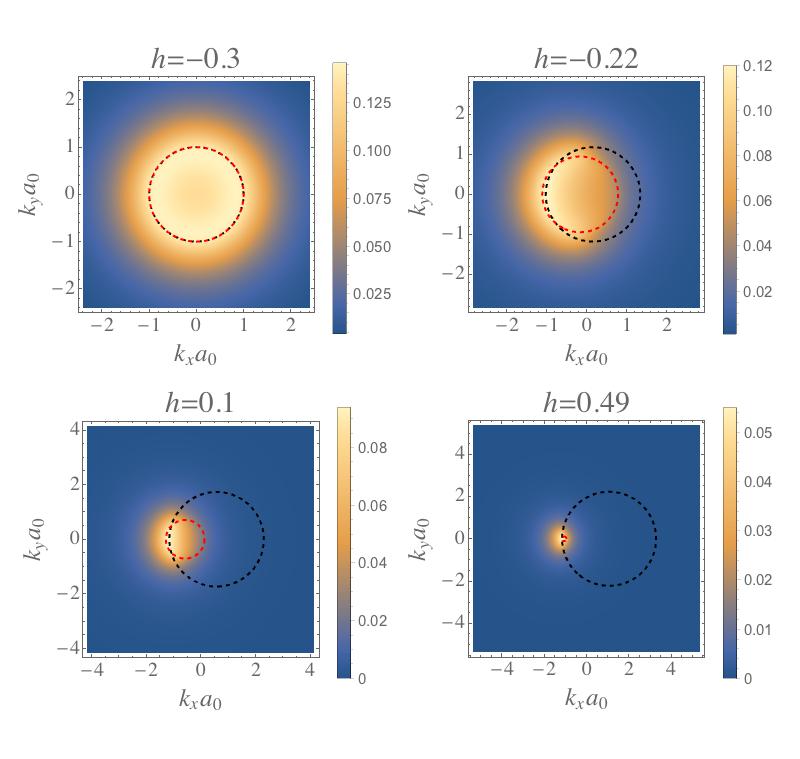
Figure 6: (Color online.) Gap function $\Delta_{\mathbf{k}\mathbf{Q}}$ at chemical potential $\mu=0.5$ for $m_{h}/m_{e}=4$, $k_{\text{TF}}a_{0}=0.1$. Top left: the uniform ($Q=0$) SF phase. Top right and bottom left and right: FF states. Dashed lines: the normal state Fermi surfaces shifted by $\pm\mathbf{Q}/2$ to touch at energetically degenerate points. Hole Fermi surface (red, smaller): $\xi_{-\mathbf{k}+\frac{\mathbf{Q}}{2},h}=0$. Electron Fermi surface (black, larger): $\xi_{\mathbf{k}+\frac{\mathbf{Q}}{2},e}=0$.

We can also ask about the behavior of the ordering wavevector $\mathbf{Q}$. Naively, one expects that electrons at the electron Fermi surface with wavevector $k_{\text{F}e}$ will pair with holes at the hole Fermi surface with wavevector $k_{\text{F}h}$ because they are degenerate in energy. This would mean that $|\mathbf{Q}|=|k_{\text{F}h}-k_{\text{F}e}|$. This is the case for neutral atoms with contact interactions in two dimensions and at the SF-Normal phase boundary in three dimensions. We find that the ordering wavevector in mean-field theory is below this naive value. The deviation is clearest at weak screening (Fig. 5). We believe that this is because the interaction $V_{\bf q}$ increases with decreasing $|{\bf q}|$. So, the exciton may gain attractive energy by pairing at a lower wavevector than the one expected from considering the kinetic energy alone.

Fig. 6 shows how the gap function evolves for the case of $\mu=0.5$, compared with the underlying normal-state Fermi surfaces (shifted by $\pm\mathbf{Q}/2$ so that they touch at the points where they are degenerate). At $h=-0.3$, the system is in the $Q=0$ SF state (top right). The order parameter has $s$-wave symmetry, and decays quickly outside of the normal-state Fermi surface. As we increase the bias, the system enters a FF state. The order parameter jumps from being $s$-wave to being peaked only on the side of $\mathbf{k}$-space where the shifted Fermi surfaces are closest (top right). As the bias $h$ is moved further into the FF phase, the region in which the order parameter is peaked reduces (bottom left). It still remains peaked in the region where the shifted Fermi surfaces are closest. Eventually, just below the FFLO-Normal phase transition, it is peaked only around the spot where the two shifted Fermi surfaces almost touch (bottom right).

Figure 7: Ground states of the electron-hole bilayer as a function of electron separation $r_{s}$ and fractional density imbalance $(n_{h}-n_{e})/(n_{h}+n_{e})$ at layer separation $d=a_{0}$. SF shows where a zero-momentum $\mathbf{Q}=0$ superfluid is found when there are equal numbers of electrons and holes, FFLO labels region of exciton condensation at nonzero momenta ($\mathbf{Q}\neq 0$), PS: phase separation. PP labels regions of partially polarized normal state. Left panels are for $\alpha=m_{h}/m_{e}=1$ with screening wavevectors $k_{\text{TF}}a_{0}=0.1$ and 0.5. Right panels are for $\alpha=4$ with $k_{\text{TF}}a_{0}=0.1$ and 1.0. Parts of the FFLO-PP boundary are extrapolated (dashed line) because this corresponds to very small regions in $\mu$-$h$ space and we do not have the numerical resolution to determine the boundary precisely.

For further comparison with the literature, we also plot in Fig. 7 the phase diagram in density space, in terms of $r_{s}=(2/\pi n)^{1/2}a_{0}$ and the density imbalance, $\delta n/n$, as obtained from Eq. (9). As mentioned above, there is a region of phase separation at large $r_{s}$ and low imbalance. At lower $r_{s}$, we find a partially polarized normal phase (PP) at $\alpha=4$ and $k_{\text{TF}}a_{0}=1$. We note that we see a larger FFLO region when the majority carrier has the higher mass compared with the case when the minority carrier has the higher mass, in agreement with Parish et al. (2011).

In summary, we reviewed the mean field theory for electron-hole bilayer for a screened Coulomb interaction. We do not find Sarma phases in the experimentally realistic setup where the bilayer is connected to normal leads. We should note that our model has not considered intralayer repulsion and, in principle, that may affect our conclusion. We also disagree with Yamashita et al Yamashita et al. (2010) and do not find a large region in the phase diagram with a partially polarized normal ground state for screened or unscreened interactions.

We have assumed that the state with a non-zero ordering wavevector is a Fulde-Ferrell state. This analysis is valid near the FFLO-normal phase boundaries of the system. We can ask whether the system prefers to condense into excitonic states with two (Larkin-Ovchinnikov) or more ordering wavevectors. We now move on to address this issue, at least near the FFLO-normal boundary.

V Ginzbury-Landau theory for the onset of excitonic pairing

We will now abandon the self-consistent mean-field theory of the system and turn to the Ginzburg-Landau treatment in the literature, first introduced for spin-polarized superconductors Larkin and Ovchinnikov (1965); Shimahara (1998) and later adapted to bilayers Lozovik and Yudson (1975); Szymanska et al. (2003); Combescot and Mora (2005). We review the derivation of the free energy of the system near a FFLO-normal phase boundary as a Taylor expansion in the gap function $\Delta_{\mathbf{k}\mathbf{Q}}$. This is consistent with the mean-field result that the transition is continuous in $\Delta_{\mathbf{k}\mathbf{Q}}$ at this boundary. To determine the onset of the pairing instability, we only need a Ginzburg-Landau expansion up to second order in the order parameter. We will describe this expansion in this section. This will set the scene for the next section where we calculate the fourth-order expansion for the determination of the structure of the FFLO phase.

Instead of considering only the FF state as in the previous section, we will consider pairing at multiple exciton momenta $\mathbf{Q}$ in the Ginzburg-Landau theory. This gives a simpler treatment of the FFLO state that would distinguish different forms of this state. In other words, we will now allow for the gap function $\Delta_{\mathbf{k}\mathbf{Q}}$ being nonzero for a discrete set of wavevectors $\mathbf{Q}$.

We start with the pairing Hamiltonian (III) and write the imaginary-time action as:

$$\begin{split}S_{\text{MF}}=\beta F_{\Delta}+\int_{0}^{\beta}\!\!\!\!d\tau\!\sum_{\mathbf{p}\mathbf{p}^{\prime}}\overline{\Psi}_{\mathbf{p}}(\tau)\,\hat{\mathbf{G}}^{-1}_{\mathbf{p}\mathbf{p}^{\prime}}\,\Psi_{\mathbf{p}^{\prime}}(\tau)\\ \end{split}$$ (10)

where the fermion fields have been written as Nambu spinors: $\Psi_{\mathbf{p}}=\left(\psi_{\mathbf{p}h},\overline{\psi}_{\mathbf{p}e}\right)^{\text{T}}$, and $\hat{\mathbf{G}}^{-1}=\hat{\mathbf{g}}^{-1}+\hat{\mathbf{\Delta}}$ with

$$\begin{split}\hat{\mathbf{g}}_{\mathbf{p}\mathbf{p}^{\prime}}^{-1}&=\begin{pmatrix}\partial_{\tau}+\xi_{\mathbf{p}h}&0\\ 0&\partial_{\tau}-\xi_{\mathbf{p}e}\end{pmatrix}\,\delta_{\mathbf{p}\mathbf{p}^{\prime}}\,,\\ \hat{\mathbf{\Delta}}_{\mathbf{p}\mathbf{p}^{\prime}}&=\sum_{\mathbf{Q}}\begin{pmatrix}0&\Delta_{\frac{\mathbf{p}^{\prime}-\mathbf{p}}{2},\mathbf{Q}}\\ \overline{\Delta}_{\frac{\mathbf{p}^{\prime}-\mathbf{p}}{2},\mathbf{Q}}&0\end{pmatrix}\,\delta_{\mathbf{p}+\mathbf{p}^{\prime},\mathbf{Q}}\,.\end{split}$$ (11)

Tracing out the fermion fields gives us an action as a functional of the pairing fields $\Delta_{\mathbf{k}\mathbf{Q}}$ which can be formally written as $S=\beta F_{\Delta}-\ln\text{Det}\,\hat{\mathbf{G}}=\beta F_{\Delta}+\mathrm{Tr}\ln\hat{\mathbf{G}}^{-1}$ where $\mathrm{Tr}$ traces over not only the Nambu components but also the wavevector and Matsubara-frequency components of the fields. We can write $\mathrm{Tr}\ln\hat{\mathbf{G}}^{-1}=\mathrm{Tr}\ln\hat{\mathbf{g}}^{-1}+\mathrm{Tr}\ln(1+\hat{\mathbf{g}}\hat{\mathbf{\Delta}})$ so that the first term contributes to the normal-state free energy $F_{N}$ while the second term can be expanded in powers of $\hat{\mathbf{g}}\hat{\mathbf{\Delta}}$ when the gap function is small. The fact that $\hat{\mathbf{g}}\hat{\mathbf{\Delta}}$ is a purely off-diagonal matrix means that only terms with even powers of $\hat{\mathbf{g}}\hat{\mathbf{\Delta}}$ have a non-zero trace. Thus, we find $F=F_{N}+\delta F$ where the second term can be formally written as

$$\delta F=F_{\Delta}+\frac{1}{\beta}\sum_{l=1}^{\infty}\frac{1}{2l}\mathrm{Tr}[(\hat{\mathbf{g}}\hat{\mathbf{\Delta}})^{2l}]\,.$$ (12)

Let us consider first the term ($l=1$) that is second order in the gap function. Diagrammatically, this represents an exciton with total momentum $\mathbf{Q}$ breaking up into a virtual electron and a virtual hole before recombining again:

$$\frac{1}{2\beta}\mathrm{Tr}[(\hat{\mathbf{g}}\hat{\mathbf{\Delta}})^{2}]=\frac{1}{\beta}\!\!\sum_{\mathbf{p}\mathbf{p}^{\prime}\mathbf{Q}\omega_{n}}\!\!\frac{\left|\Delta_{(\mathbf{p}^{\prime}-\mathbf{p})/2,\mathbf{Q}}\right|^{2}\delta_{\mathbf{p}+\mathbf{p}^{\prime},\mathbf{Q}}}{(i\omega_{n}+\xi_{\mathbf{p}h})(i\omega_{n}-\xi_{\mathbf{p}^{\prime}e})}\,.$$ (13)

Hence, we find that the second-order contributions to the free energy $\delta F$ is given by

$$\begin{split}\delta F^{(2)}&=\sum_{\mathbf{k}\mathbf{k}^{\prime}\mathbf{Q}}\overline{\Delta}_{\mathbf{k}\mathbf{Q}}\left(V^{-1}_{\mathbf{k}\mathbf{k}^{\prime}}-\Pi_{\mathbf{k}\mathbf{Q}}\delta_{\mathbf{k}\mathbf{k}^{\prime}}\right)\Delta_{\mathbf{k}^{\prime}\mathbf{Q}}\,,\\ \Pi_{\mathbf{k}\mathbf{Q}}&=\frac{1-f_{D}(\xi_{-\mathbf{k}+\frac{\mathbf{Q}}{2}h})-f_{D}(\xi_{\mathbf{k}+\frac{\mathbf{Q}}{2}e})}{\xi_{-\mathbf{k}+\frac{\mathbf{Q}}{2}h}+\xi_{\mathbf{k}+\frac{\mathbf{Q}}{2}e}}\end{split}$$ (14)

From this, we can deduce that the system has an instability to excitonic pairing at a wavevector $\mathbf{Q}$ if ${\tilde{V}}^{-1}_{\mathbf{k}\mathbf{k}^{\prime}\mathbf{Q}}\equiv V^{-1}_{\mathbf{k}\mathbf{k}^{\prime}}-\Pi_{\mathbf{k}\mathbf{Q}}\delta_{\mathbf{k}\mathbf{k}^{\prime}}$ (as a matrix in its momentum indices, $\mathbf{k}$ and $\mathbf{k}^{\prime}$) has a negative eigenvalue. It can be shown that this result is identical to the onset of the FF instability predicted by the gap equation (III). As for the choice of ordering wavevector at the FFLO-normal boundary, the system should pick the wavevector $\mathbf{Q}$ that produces the first negative eigenvalue for ${\tilde{V}}^{-1}$ as we lower the bias field $|h|$ from $\mu$. The corresponding eigenvector $v_{\mathbf{k}\mathbf{Q}}$ provides the gap function $\Delta_{\mathbf{k}\mathbf{Q}}$ of this state up to an overall $\mathbf{k}$-independent factor. As in any Landau theory, the magnitude of the order parameter (gap function here) can only be determined after we have calculated positive terms fourth order in order parameter in the free energy (see below).

Due to the isotropy of the interaction, the eigenvalues ${\tilde{V}}^{-1}$ are only functions of $Q\equiv|\mathbf{Q}|$. Thus, this analysis only tells us the magnitude $Q_{c}$ of the ordering wavevector at the FFLO-normal boundary. Moreover, $\delta F^{(2)}$ does not mix up the pairing fields at different wavevectors. This means that, to this quadratic level in the order parameter, the Ginzburg-Landau theory cannot tell us whether the system condenses into a FF state (condensation at a single $\mathbf{Q}$), LO state (condensation at $\pm\mathbf{Q}$) or other states with more ordering wavevectors with the same magnitude. Put another way, all these possible FFLO states are degenerate in energy at the FFLO-normal boundary, provided that it is a continuous transition ($\Delta_{\mathbf{k}\mathbf{Q}}\to 0$). We will show in the next section that the fourth-order terms can lift this degeneracy.

VI Structure of the excitonic state near the FFLO-normal boundary

Having outlined the second-order expansion of the Ginzburg-Landau free energy in the previous section, we now proceed to obtain a fourth-order expansion. This is needed to determine the relative free energies of different FFLO states near the FFLO-normal boundary. Our methodology is similar to Shimahara Shimahara (1998).

The second-order analysis has already determined the magnitude of the possible ordering wavevectors $Q_{c}$. We will now work with only the pairing fields at those wavevectors.

$$\Delta_{\mathbf{k}\mathbf{Q}}=\sum_{i}\Delta_{i}v_{\mathbf{k}i}\delta_{\mathbf{Q},\mathbf{Q}_{i}}\,,\qquad\sum_{\mathbf{k}}|v_{\mathbf{k}i}|^{2}=1$$ (15)

where $v_{\mathbf{k}i}$ is the normalized eigenvector of ${\tilde{V}}^{-1}_{\mathbf{k}\mathbf{k}^{\prime}}$ at wavevector $\mathbf{Q}_{i}$ and $i$ labels the members of the discrete set of ordering wavevectors. We will restrict our attention to the FF state (single $\mathbf{Q}$), LO state ($i=\pm$: $\mathbf{Q}_{+}=-\mathbf{Q}_{-}=\mathbf{Q}$) and the state with square symmetry ($i=\pm x,\pm y$: $\mathbf{Q}_{x}=-\mathbf{Q}_{-x}=(Q_{c},0)$, $\mathbf{Q}_{y}=-\mathbf{Q}_{-y}=(0,Q_{c})$ in Cartesian coordinates).

The fourth-order contributions to the free energy involve the evaluation of $\mathrm{Tr}[(\hat{\mathbf{g}}\hat{\mathbf{\Delta}})^{4}]$. Physically, this involves two excitons breaking up and exchanging virtual electrons and holes. The expressions for these contributions are cumbersome and are presented in Appendix B. From the parametrization (15) and the expression (25), the Ginzburg-Landau free energy for the FF state near the phase boundary to the normal state can be written in the form:

$$\delta F_{\textrm{FF}}={\tilde{r}}_{c}|\Delta|^{2}+b_{\textrm{FF}}|\Delta|^{4}$$ (16)

where ${\tilde{r}}_{c}<0$ is the most negative eigenvector of ${\tilde{V}}^{-1}$. For the FF state, there is only one ordering wavevector and the Hamiltonian is invariant under a global phase shift for the electrons and the holes. Thus, $\delta F_{\textrm{FF}}$ is insensitive to the phase of $\Delta_{\mathbf{k}\mathbf{Q}}$. The system would spontaneously break this U(1) phase as a signature of excitonic superfluidity.

The LO free energy [from Eq. (27)] is given by

$$\delta F_{\textrm{LO}}=\sum_{i=\pm}\!\left({\tilde{r}}_{c}|\Delta_{i}|^{2}+b_{\textrm{FF}}|\Delta_{i}|^{4}\right)+b_{\textrm{LO}}|\Delta_{+}|^{2}|\Delta_{-}|^{2}\,.$$ (17)

We note that the order parameters, $\Delta_{+}$ and $\Delta_{-}$, should have the same magnitude because ${\tilde{r}}_{c}$ is only a function of the magnitude of the ordering wavevector. In addition to the overall phase, the free energy is also insensitive to the relative phase between $\Delta_{+}=\Delta e^{i\chi/2}$ and $\Delta_{-}=\Delta e^{-i\chi/2}$. This insensitivity of the free energy to the relative phase $\chi$ is simply the consequence of translational invariance. We can see this from the form of the order parameter in real space: $\Delta_{\textrm{LO}}(\mathbf{r})=2\Delta\cos(\mathbf{Q}\cdot\mathbf{r}+\chi)$. The LO state should spontaneously break this symmetry as the system develops spatial density modulations.

For the square state with four ordering wavevectors, the free energy (30) can be written in the form:

$$\delta F_{\textrm{sq}}=\!\!\!\sum_{i=\pm x,\pm y}\!\!\! \left({\tilde{r}}_{c}|\Delta_{i}|^{2}+b_{\textrm{FF}}|\Delta_{i}|^{4}\right)+b_{\textrm{LO}}\!\!\!\sum_{j=x,y}\!\!|\Delta_{j}|^{2}|\Delta_{-j}|^{2}$$

$$+b_{\textrm{sq}}\,(|\Delta_{x}|^{2}|\Delta_{y}|^{2}+|\Delta_{-x}|^{2}|\Delta_{-y}|^{2})$$

$$+c_{\textrm{sq}}\,(\Delta_{x}\Delta_{-x}\overline{\Delta}_{y}\overline{\Delta}_{-y}+\text{c.c.})\,.$$ (18)

Again, we see that the free energy is invariant under an overall phase shift, or relative phase shifts of the form $\Delta_{\pm x}\to\Delta_{\pm x}e^{\pm i\chi_{x}}$ and similarly for $x\to y$. This leaves one phase degree of freedom which can be chosen to minimize the term with coefficient $c_{\textrm{sq}}$ in $\delta F_{\textrm{sq}}$. Denoting the complex order parameters as $\Delta_{i}=|\Delta|e^{i\theta_{i}}$, we want $\theta_{x}+\theta_{-x}-\theta_{y}-\theta_{-y}=0$ or $\pi$ depending on whether $c_{\textrm{sq}}$ is negative or positive. We find numerically that $c_{\textrm{sq}}<0$ so that the ground state should have $\theta_{x}+\theta_{-x}=\theta_{y}+\theta_{-y}$.

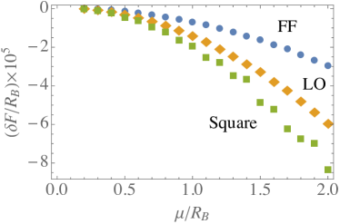
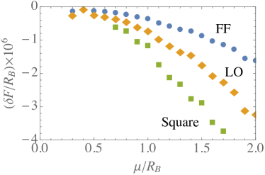
Figure 8: (Color online.) The free energy difference per unit area between the FFLO and normal states near the FFLO-normal phase boundaries (upper panel is for majority holes, lower panel is for majority electrons) over a range of chemical potentials $\mu$. ($\alpha=m_{h}/m_{e}=4$, $k_{\text{TF}}a_{0}=0.1$.)

Having established the free energy up to fourth order in the order parameter, we can discuss the relative stability of these states. Figure 8 shows the general behavior for all the parameters we have explored — the square state is energetically favorable compared with the FF or LO states.

It is interesting to compare our results with those of Parish et al. Parish et al. (2011) who worked in the limit of extreme electron-hole imbalance. In that work, by writing down a phenomenological Ginzburg-Landau theory for weak crystallization, the authors also found that condensation into two pairs of wavevectors is favorable compared with condensation into a single wavevector or a pair of opposite wavevectors. We agree with this conclusion and have extended the phase boundary away from the limit of extreme electron-hole imbalance. On the other hand, that work obtained a different phase relationship between $\Delta_{x}$ and $\Delta_{y}$, giving a $\pi/2$ phase difference between the two order parameters. This originated from an assumption that $c_{\textrm{sq}}>0$ in Eq. (VI). As discussed above, our calculation gives $c_{\textrm{sq}}<0$ and so our ground state does not agree with Parish et al. (2011). We believe that the Ginzburg-Landau calculation has shown that the phenomenological free energy of Parish et al. (2011) assumed more symmetry than is allowed by the microscopic system after excitonic condensation.

Finally, we note that these energies differences are very small: $\sim 10^{-6}R_{B}$ near the phase boundary. This can be compared with the condensation energy of the FFLO state $\sim 10^{-2}R_{B}$ (from Fig. 3, right). This suggests that we may observe an FFLO phase at temperatures of the order of 0.5K, but the ground-state geometry would be not be observed at all temperatures down to 0.1 mK. Between these two temperatures, we believe that the crystalline structure of the ground state would be melted and may be described by a nematic phase Radzihovsky and Vishwanath (2009).

VII Discussion

We investigate the possibility of excitonic superfluidity in electron-hole bilayers. Our phase diagram of the system covers the the whole range of electron-hole density imbalance and for different degrees of Coulomb screening.

We do not find Sarma phases in the experimentally realistic setup where the bilayer is connected to normal leads. We are also able to comment on the disagreement in the literature on the stability of a partially polarized normal state. We are able to cover the parameter space covered by the extremely imbalanced system discussed by Parish et al. Parish et al. (2011), and the work of Yamashita et al. Yamashita et al. (2010). Our results show that the partially polarized state only exists in a narrow region on the phase diagram near the fully polarized state. There is no wide region of stability as claimed by Yamashita et al..

Our Ginzburg-Landau treatment allows us to investigate the stability of the different forms of the pairing state near the onset of FFLO superfluidity. We investigated several candidate ground states: the Fulde-Ferrell (FF) state with a single pairing wavevector, the Larkin-Ovchinnikov (LO) state with a pair of opposite pairing wavevectors giving rise to a density wave in one dimension, and also the pairing of electrons and holes at several ordering wavevectors. We find that the energetics favor a state with spontaneously breaking translational symmetry in two dimensions. However, the energy scales involved in differentiating between different two-dimensional spatial structure in such a state is small and might be hard to detect under thermal and quantum fluctuations.

Appendix A Gap Equation for the Exciton Superfluid

Consider first the Fulde-Ferrell state where electrons at wavevector $-\mathbf{k}+\mathbf{Q}/2$ pair up with holes at $\mathbf{k}+\mathbf{Q}/2$ for a single $\mathbf{Q}$. The imaginary-time action corresponding to the mean-field Hamiltonian $H_{\text{pair}}$ (III) can be written in the compact form:

$$S_{\text{MF}}=\beta F_{\Delta}+\frac{1}{\beta}\sum_{k}\overline{\Psi}_{k\mathbf{Q}}\mathbf{G}_{k\mathbf{Q}}^{-1}\Psi_{k\mathbf{Q}}$$ (19)

where $F_{\Delta}$ is defined in Eq. (III), $\beta=\hbar/k_{\rm B}T$ and $T$ is the temperature. The fermion fields have been rewritten using the Nambu spinor notation, $\Psi_{{k\mathbf{Q}}}=\left(\psi_{-\mathbf{k}+\mathbf{Q}/2,h},\overline{\psi}_{\mathbf{k}+\mathbf{Q}/2,e}\right)^{\rm T}$ and then a Fourier transform to Matsubara frequencies has been performed: $\Psi_{\mathbf{k}\sigma}(\tau)=\beta^{-1}\sum_{n}\Psi_{k\sigma}e^{-i\omega_{n}\tau}$ with $k=(\mathbf{k},\omega_{n})$ and $\omega_{n}=(2n+1)\pi/\beta$ with integer $n$. The inverse Green’s function is a function of the pairing field $\Delta_{\mathbf{k}}$:

$$\mathbf{G}^{-1}_{k\mathbf{Q}}=\begin{pmatrix}-i\omega_{n}+\xi_{-\mathbf{k}+\frac{\mathbf{Q}}{2}h}&\Delta_{\mathbf{k}\mathbf{Q}}\\ \overline{\Delta}_{\mathbf{k}\mathbf{Q}}&-i\omega_{n}-\xi_{\mathbf{k}+\frac{\mathbf{Q}}{2}e}\end{pmatrix}\,.$$ (20)

The poles of this Green’s function in frequency space, i.e. the values of $i\omega_{n}$ for which the determinant of $\mathbf{G}^{-1}$ vanishes, are found at $i\omega_{n}={\cal E}_{\mathbf{k}\mathbf{Q}}^{+}$ and $-{\cal E}_{\mathbf{k}\mathbf{Q}}^{-}$ as given by Eq. (III).

The action is quadratic in the fermion fields which can be integrated out to give the collective field action

$$S_{\rm MF}[\Delta,\overline{\Delta}]=\beta F_{\Delta}-\sum_{k}\mathrm{Tr}\ln\mathbf{G}^{-1}_{{k\mathbf{Q}}}\,.$$ (21)

where the trace is taken over the 2$\times$2 Nambu structure. We now take the saddle-point approximation and choose $\Delta_{\mathbf{k}}$ such that it minimizes the free energy $F_{\text{MF}}=-\beta^{-1}\ln Z_{\rm MF}$ where $Z_{\text{MF}}$ is the partition function for the mean-field Hamiltonian. It can be shown that

$$F_{\text{MF}}=F_{\Delta}+\sum_{\mathbf{k}}\xi_{\mathbf{k}+\frac{\mathbf{Q}}{2}e}\!-\frac{1}{\beta}\sum_{k}\ln\det\mathbf{G}^{-1}_{k\mathbf{Q}}\,.$$ (22)

The frequency sum in the final term can be performed to give, up to terms that do not depend on $\Delta_{\mathbf{k}}$,

$$F_{\text{MF}}=F_{\Delta}\!+\!\sum_{\mathbf{k}}(\xi^{+}_{{\mathbf{k}\mathbf{Q}}}-E_{{\mathbf{k}\mathbf{Q}}})-\frac{1}{\beta}\!\sum_{\mathbf{k}\genfrac{}{}{0.0pt}{2}{\alpha}{=}\pm}\!\ln(1+e^{-\beta{\cal E}_{\mathbf{k}\mathbf{Q}}^{\alpha}})\,.$$ (23)

Thus, minimizing this free energy with respect to $\Delta_{\mathbf{k}\mathbf{Q}}$ gives a self-consistent equation for the pairing field (gap function), analogous to the gap equation in BCS theory:

$$\Delta_{\mathbf{k}}=\sum_{\mathbf{k}^{\prime}}\frac{V_{\mathbf{k}-\mathbf{k}^{\prime}}\Delta_{\mathbf{k}^{\prime}}}{2E_{\mathbf{k}^{\prime}}}\!\left[1-f_{D}({\cal E}_{\mathbf{k}^{\prime}\mathbf{Q}}^{+})-f_{D}({\cal E}_{\mathbf{k}^{\prime}\mathbf{Q}}^{-})\right]$$ (24)

where $f_{D}(E)$ is the Fermi-Dirac distribution with energy $E$ measured from the chemical potential. This equation is the same as equation (III).

Let us briefly comment on the mean-field theory for a Larkin-Ovchinnikov (LO) state where we have two pairing fields $\Delta_{\mathbf{k}\mathbf{Q}}$ and $\Delta_{\mathbf{k},-\mathbf{Q}}$. The pairing Hamiltonian (III) is still quadratic in the fermion operators. However, the Hamiltonian does not break down into independent 2$\times$2 blocks involving pairs of momenta. For instance, a hole at wavevector $-\mathbf{k}+\mathbf{Q}/2$ can be created with an electron at $\mathbf{k}+\mathbf{Q}/2$ by a term $\Delta_{\mathbf{k}\mathbf{Q}}\psi^{\dagger}_{-\mathbf{k}+\frac{\mathbf{Q}}{2},h}\psi^{\dagger}_{\mathbf{k}+\frac{\mathbf{Q}}{2},e}$ in $H_{\text{pair}}$ to form a pair with total momentum $\mathbf{Q}$. At the same time, it can also be created with an electron at $\mathbf{k}-3\mathbf{Q}/2$ by a term $\Delta_{\mathbf{k}^{\prime},-\mathbf{Q}}\psi^{\dagger}_{-\mathbf{k}^{\prime}-\frac{\mathbf{Q}}{2},h}\psi^{\dagger}_{\mathbf{k}^{\prime}-\frac{\mathbf{Q}}{2},e}$ with $\mathbf{k}^{\prime}=\mathbf{k}-\mathbf{Q}$ to form a pair with momentum $-\mathbf{Q}$. The former electron state is then coupled a hole state at $-\mathbf{k}-3\mathbf{Q}/2$ forming a pair at $-\mathbf{Q}$ and the latter electron state is coupled to a hole state at $-\mathbf{k}+5\mathbf{Q}/2$ forming a pair at $\mathbf{Q}$. Thus, electron states are coupled to other electron states with wavevectors separated by multiples of $2\mathbf{Q}$ and similarly for holes. This is simply a consequence of the fact that the LO state has density variations in space with wavevector $2\mathbf{Q}$£. In other words, the eigenstates of the mean-field Hamiltonian for the LO state form Bloch bands. Results can be obtained numerically instead of analytically.

Appendix B Fourth-Order Contributions to the Ginzburg-Landau Free Energy

The fourth-order contributions to the free energy involve the evaluation of $\mathrm{Tr}[(\hat{\mathbf{g}}\hat{\mathbf{\Delta}})^{4}]$. Physically, this involves two excitons breaking up and exchanging virtual electrons and holes. For the Fulde-Ferrell state, there is only one type of exciton involved with momentum $\mathbf{Q}$ and so the virtual states all involve holes with momentum $-\mathbf{k}+\mathbf{Q}/2$ and electrons with momentum $\mathbf{k}+\mathbf{Q}/2$.

$$\delta F^{(4)}_{\textrm{FF}}=\frac{1}{\beta}\!\sum_{\mathbf{k}\omega_{n}}\frac{|\Delta_{\mathbf{k}\mathbf{Q}}|^{4}}{(i\omega_{n}+\xi_{-\mathbf{k}+\frac{\mathbf{Q}}{2}h})^{2}(i\omega_{n}-\xi_{\mathbf{k}+\frac{\mathbf{Q}}{2}e})^{2}}=\sum_{\mathbf{k}}|\Delta_{\mathbf{k}\mathbf{Q}}|^{4}\frac{1-f_{D}(\xi_{-\mathbf{k}+\frac{\mathbf{Q}}{2}h})-f_{D}(\xi_{\mathbf{k}+\frac{\mathbf{Q}}{2}e})}{(\xi_{-\mathbf{k}+\frac{\mathbf{Q}}{2}h}+\xi_{\mathbf{k}+\frac{\mathbf{Q}}{2}e})^{3}}\,.$$ (25)

For the Larkin-Ovchinnikov state, there are two types of excitons. In addition to virtual states involving holes at momentum $-\mathbf{k}\pm\mathbf{Q}/2$ and electrons at momentum $\mathbf{k}\pm\mathbf{Q}/2$, virtual states with hole momentum $-\mathbf{k}\pm 3\mathbf{Q}/2$ and electron momentum $\mathbf{k}\pm 3\mathbf{Q}/2$ are involved. For instance, a hole with momentum $-\mathbf{k}+\mathbf{Q}/2$ from an exciton with momentum $\mathbf{Q}$ may pair up with an electron with momentum $\mathbf{k}^{\prime}+\mathbf{Q}/2$ from another exciton of the same momentum $\mathbf{Q}$. If they form an exciton with momentum $-\mathbf{Q}$, then we need $\mathbf{k}^{\prime}=\mathbf{k}-2\mathbf{Q}$ so that the electron momentum is $\mathbf{k}^{\prime}-\mathbf{Q}/2=\mathbf{k}-3\mathbf{Q}/2$. We can interpret this physically as arising from the spatial exciton density variation in the LO state: $|\Delta(\mathbf{r})|^{2}\sim\cos^{2}(\mathbf{Q}\cdot\mathbf{r}+\chi)$ causing Bragg diffraction of electrons and holes. It can be shown that the fourth-order contribution to the free energy, $\delta F^{(4)}_{\textrm{LO}}$, contains $2\delta F^{(4)}_{\textrm{FF}}$ and two extra terms $\delta F^{(4)}_{++--}$ and $2\delta F^{(4)}_{+--+}$ arising from the order in which $\pm Q$ components of $\hat{\mathbf{\Delta}}$ were involved in the four $\hat{\mathbf{\Delta}}$ in evaluation of $\mathrm{Tr}[(\hat{\mathbf{g}}\hat{\mathbf{\Delta}})^{4}]$:

$$\delta F^{(4)}_{+--+}=\frac{1}{\beta}\!\sum_{\mathbf{k}\omega_{n}}\frac{|\Delta_{\mathbf{k}\mathbf{Q}}|^{2}|\Delta_{\mathbf{k}+\mathbf{Q},-\mathbf{Q}|}|^{2}}{(i\omega_{n}+\xi_{1h})(i\omega_{n}-\xi_{1e})(i\omega_{n}+\xi_{2h})}\,,\qquad\delta F^{(4)}_{++--}=\frac{1}{\beta}\!\sum_{\mathbf{k}\omega_{n}}\frac{|\Delta_{\mathbf{k}\mathbf{Q}}|^{2}|\Delta_{\mathbf{k}-\mathbf{Q},-\mathbf{Q}|}|^{2}}{(i\omega_{n}+\xi_{1h})(i\omega_{n}-\xi_{1e})(i\omega_{n}-\xi_{2e})}$$ (26)

where $\xi_{1h}=\xi_{-\mathbf{k}+\frac{\mathbf{Q}}{2}h}$, $\xi_{1e}=\xi_{\mathbf{k}+\frac{\mathbf{Q}}{2}h}$, $\xi_{2h}=\xi_{-\mathbf{k}+\frac{3\mathbf{Q}}{2},h}$ and $\xi_{2e}=\xi_{\mathbf{k}+\frac{3\mathbf{Q}}{2}e}$. At zero temperature, this gives

$$\delta F^{(4)}_{\textrm{LO}}=2\delta F^{(4)}_{\textrm{FF}}+2\delta F^{(4)}_{++--}+2\delta F^{(4)}_{+--+}\,,$$ (27)

$$\begin{split}\hbox to0.0pt{$\displaystyle\delta F^{(4)}_{+--+}=\frac{1}{2}\sum_{\mathbf{k}}|\Delta_{\mathbf{k}\mathbf{Q}}|^{2}|\Delta_{\mathbf{k}+\mathbf{Q},-\mathbf{Q}}|^{2}$\hss}\\ &\qquad\bigg{[}\frac{\Theta(\xi_{1h})}{(\xi_{1e}+\xi_{1h})^{2}(\xi_{2h}-\xi_{1h})}+\frac{\Theta(\xi_{2h})}{(\xi_{2h}+\xi_{1e})^{2}(\xi_{1h}-\xi_{2h})}-\frac{\Theta(-\xi_{1e})}{(\xi_{1e}+\xi_{1h})^{2}(\xi_{1e}+\xi_{2h})}-\frac{\Theta(-\xi_{1e})}{(\xi_{1e}+\xi_{2h})^{2}(\xi_{1e}+\xi_{1h})}\bigg{]}\end{split}$$ (28)

$$\begin{split}\hbox to0.0pt{$\displaystyle\delta F^{(4)}_{++--}=\frac{1}{2}\sum_{\mathbf{k}}|\Delta_{{\mathbf{k}\mathbf{Q}}}|^{2}|\Delta_{\mathbf{k}-\mathbf{Q},-\mathbf{Q}}|^{2}$\hss}\\ &\qquad\bigg{[}\frac{\Theta(-\xi_{1e})}{(\xi_{1e}+\xi_{1h})^{2}(\xi_{1e}-\xi_{2e})}+\frac{\Theta(-\xi_{2e})}{(\xi_{2e}+\xi_{1h})^{2}(\xi_{2e}-\xi_{1e})}+\frac{\Theta(\xi_{1h})}{(\xi_{1h}+\xi_{1e})^{2}(\xi_{1h}+\xi_{2e})}+\frac{\Theta(\xi_{1h})}{(\xi_{1h}+\xi_{2e})^{2}(\xi_{1h}+\xi_{1e})}\bigg{]}\end{split}$$ (29)

For the square state, the excitons have momenta $\pm\mathbf{Q}_{x}=(\pm Q,0)$ and $\pm\mathbf{Q}_{y}=(0,\pm Q)$. The fourth-order contributions to the energy at zero temperature are

$$\delta F^{(4)}_{\textrm{sq}}=4(\delta F^{(4)}_{\textrm{FF}}+\delta F^{(4)}_{++--}+\delta F^{(4)}_{+--+})+8(\delta F^{(4)}_{xxyy}+\delta F^{(4)}_{xyyx})+4\delta F^{(4)}_{xy-x-y}\,,$$ (30)

$$\begin{split}\hbox to0.0pt{$\displaystyle\delta F^{(4)}_{xxyy}=\frac{1}{2}\sum_{\mathbf{k}}|\Delta_{\mathbf{k}\mathbf{Q}_{x}}|^{2}|\Delta_{\mathbf{k}+(\mathbf{Q}_{y}-\mathbf{Q}_{x})/2,\mathbf{Q}_{y}}|^{2}$\hss}\\ &\qquad\bigg{[}\frac{\Theta(-\xi_{1e})}{(\xi_{1e}+\xi_{1h})^{2}(\xi_{1e}-\xi_{3e})}+\frac{\Theta(-\xi_{3e})}{(\xi_{3e}+\xi_{1h})^{2}(\xi_{3e}-\xi_{1e})}+\frac{\Theta(\xi_{1h})}{(\xi_{1h}+\xi_{1e})^{2}(\xi_{1h}+\xi_{3e})}+\frac{\Theta(\xi_{1h})}{(\xi_{1h}+\xi_{3e})^{2}(\xi_{1e}+\xi_{1h})}\bigg{]}\end{split}$$ (31)

$$\begin{split}\hbox to0.0pt{$\displaystyle\delta F^{(4)}_{xyyx}=\frac{1}{2}\sum_{\mathbf{k}}|\Delta_{\mathbf{k}\mathbf{Q}_{x}}|^{2}|\Delta_{\mathbf{k}+(\mathbf{Q}_{x}-\mathbf{Q}_{y})/2,\mathbf{Q}_{y}}|^{2}$\hss}\\ &\qquad\bigg{[}\frac{\Theta(\xi_{1h})}{(\xi_{1h}+\xi_{13})^{2}(\xi_{3h}-\xi_{1h})}+\frac{\Theta(\xi_{3h})}{(\xi_{3h}+\xi_{1e})^{2}(\xi_{1h}-\xi_{3h})}-\frac{\Theta(-\xi_{1e})}{(\xi_{1h}+\xi_{1e})^{2}(\xi_{1e}+\xi_{3h})}-\frac{\Theta(-\xi_{1e})}{(\xi_{3h}+\xi_{1e})^{2}(\xi_{1h}+\xi_{1e})}\bigg{]}\end{split}$$ (32)

$$\begin{split}\hbox to0.0pt{$\displaystyle\delta F^{(4)}_{xy-x-y}=\frac{1}{2}\sum_{\mathbf{k}}\left(\Delta_{\mathbf{k}\mathbf{Q}_{x}}\overline{\Delta}_{\mathbf{k}+(\mathbf{Q}_{x}-\mathbf{Q}_{y})/2,\mathbf{Q}_{y}}\Delta_{\mathbf{k}-\mathbf{Q}_{y},-\mathbf{Q}_{x}}\overline{\Delta}_{\mathbf{k}-(\mathbf{Q}_{x}+\mathbf{Q}_{y})/2,-\mathbf{Q}_{y}}+\ \text{c.c.}\ \right)$\hss}\\ &\qquad\bigg{[}\frac{\Theta(\xi_{1h})}{(\xi_{1h}+\xi_{1e})(\xi_{1h}+\xi_{4e})(\xi_{3h}-\xi_{1h})}+\frac{\Theta(\xi_{3h})}{(\xi_{3h}+\xi_{1e})(\xi_{3h}+\xi_{4e})(\xi_{1h}-\xi_{3h})}\\ &\qquad\qquad\qquad\qquad\qquad\qquad\qquad\qquad+\frac{\Theta(-\xi_{1e})}{(\xi_{1e}+\xi_{1h})(\xi_{1e}+\xi_{3h})(\xi_{1e}-\xi_{4e})}+\frac{\Theta(-\xi_{4e})}{(\xi_{4e}+\xi_{1h})(\xi_{4e}+\xi_{3h})(\xi_{4e}-\xi_{1e})}\bigg{]}\end{split}$$ (33)

where $\xi_{1h}=\xi_{-\mathbf{k}+\frac{\mathbf{Q}_{x}}{2}h}$, $\xi_{1e}=\xi_{\mathbf{k}+\frac{\mathbf{Q}_{x}}{2}h}$, $\xi_{2h}=\xi_{-\mathbf{k}+\frac{3\mathbf{Q}_{x}}{2},h}$, $\xi_{2e}=\xi_{\mathbf{k}+\frac{3\mathbf{Q}_{x}}{2}e}$, $\xi_{3h}=\xi_{-\mathbf{k}+\mathbf{Q}_{y}-\frac{\mathbf{Q}_{x}}{2},h}$, $\xi_{3e}=\xi_{\mathbf{k}+\mathbf{Q}_{y}-\frac{\mathbf{Q}_{x}}{2},e}$ and $\xi_{4e}=\xi_{\mathbf{k}-\mathbf{Q}_{y}-\frac{\mathbf{Q}_{x}}{2},e}$.

References

- Blatt et al. (1962) J. M. Blatt, K. W. Böer, and W. Brandt, Phys. Rev. 126, 1691 (1962).
- Keldysh and Kozlov (1968) L. Keldysh and A. Kozlov, Sov. Phys. JETP 27, 521 (1968).
- Nozières and Comte (1982) P. Nozières and C. Comte, J. Physique 43, 1083 (1982).
- Moskalenko and Snoke (2000) S. A. Moskalenko and D. W. Snoke, Bose-Einstein Condensation of Excitons and Biexcitons (Cambridge University Press, 2000).
- Lozovik and Yudson (1975) Y. E. Lozovik and V. I. Yudson, JETP Lett. 22, 274 (1975).
- Littlewood and Zhu (1996) P. B. Littlewood and X. Zhu, Phys. Scr. T68, 56 (1996).
- De Palo et al. (2002) S. De Palo, F. Rapisarda, and G. Senatore, Phys. Rev. Lett. 88, 206401 (2002), arXiv:0201414v1 [arXiv:cond-mat] .
- Eastham and Littlewood (2001) P. R. Eastham and P. B. Littlewood, Phys. Rev. B 64, 235101 (2001).
- Deng et al. (2002) H. Deng, G. Weihs, C. Santori, J. Bloch, and Y. Yamamoto, Science 298, 199 (2002).
- Szymanska et al. (2003) M. H. Szymanska, P. B. Littlewood, and B. D. Simons, Phys. Rev. A 68, 013818 (2003).
- Kasprzak et al. (2006) J. Kasprzak, M. Richard, S. Kundermann, A. Baas, P. Jeambrun, J. M. J. Keeling, F. M. Marchetti, M. H. Szymańska, R. André, J. L. Staehli, V. Savona, P. B. Littlewood, B. Deveaud, and L. S. Dang, Nature 443, 409 (2006).
- Croxall et al. (2008) A. F. Croxall, K. Das Gupta, C. A. Nicoll, M. Thangaraj, H. E. Beere, I. Farrer, D. A. Ritchie, and M. Pepper, Phys. Rev. Lett. 101, 246801 (2008).
- Seamons et al. (2009) J. A. Seamons, C. P. Morath, J. L. Reno, and M. P. Lilly, Phys. Rev. Lett. 102, 026804 (2009).
- Fulde and Ferrell (1964) P. Fulde and R. A. Ferrell, Phys. Rev. 135, A550 (1964).
- Larkin and Ovchinnikov (1965) A. I. Larkin and Y. N. Ovchinnikov, Sov. Phys. JETP 20, 762 (1965).
- Sarma (1963) G. Sarma, J. Phys. Chem. Solids 24, 1029 (1963).
- Pieri et al. (2007) P. Pieri, D. Neilson, and G. C. Strinati, Phys. Rev. B 75, 113301 (2007).
- Subası et al. (2010) A. L. Subası, P. Pieri, G. Senatore, and B. Tanatar, Phys. Rev. B 81, 075436 (2010).
- Yamashita et al. (2010) K. Yamashita, K. Asano, and T. Ohashi, J. Phys. Soc. Jpn. 79, 33001 (2010).
- Parish et al. (2011) M. M. Parish, F. M. Marchetti, and P. B. Littlewood, Europhys. Lett. 95, 27007 (2011).
- Świerkowski et al. (1995) L. Świerkowski, J. Szymanski, and Z. W. Gortel, Phys. Rev. Lett. 74, 3245 (1995).
- Das Gupta et al. (2011) K. Das Gupta, A. F. Croxall, J. Waldie, C. A. Nicoll, H. E. Beere, I. Farrer, D. A. Ritchie, and M. Pepper, Advances in Condensed Matter Physics 2011, 727958 (2011).
- Neilson et al. (2014) D. Neilson, A. Perali, and A. R. Hamilton, Phys. Rev. B 89, 060502 (2014).
- Note (1) We have attempted to use an interaction based on the full form of screening in the random phase approximation, but it added significant numerical complications to our minimization calculations.
- Conduit et al. (2008) G. J. Conduit, P. H. Conlon, and B. D. Simons, Phys. Rev. A 77, 053617 (2008).
- Chandrasekhar (1962) B. S. Chandrasekhar, App. Phys. Lett. 1, 7 (1962).
- Clogston (1962) A. M. Clogston, Phys. Rev. Lett. 9, 266 (1962).
- Machida and Nakanishi (1984) K. Machida and H. Nakanishi, Phys. Rev. B 30, 122 (1984).
- Matsuo et al. (1998) S. Matsuo, S. Higashitani, Y. Nagato, and K. Nagai, J. Phys. Soc. Jpn. 67, 280 (1998).
- Forbes et al. (2005) M. M. Forbes, E. Gubankova, W. V. Liu, and F. Wilczek, Phys. Rev. Lett. 94, 017001 (2005).
- Lamacraft and Marchetti (2008) A. Lamacraft and F. M. Marchetti, Phys. Rev. B 77, 014511 (2008).
- Andrenacci et al. (1999) N. Andrenacci, A. Perali, P. Pieri, and G. C. Strinati, Phys. Rev. B 60, 12410 (1999).
- Parish et al. (2005) M. M. Parish, B. Mihaila, E. M. Timmermans, K. B. Blagoev, and P. B. Littlewood, Phys. Rev. B 71, 064513 (2005).
- Shimahara (1998) H. Shimahara, J. Phys. Soc. Jpn. 67, 736 (1998).
- Combescot and Mora (2005) R. Combescot and C. Mora, Eur. Phys. J. B 44, 189 (2005).
- Radzihovsky and Vishwanath (2009) L. Radzihovsky and A. Vishwanath, Phys. Rev. Lett. 103, 010404 (2009).