$\bm{\Lambda_{c}\to\Lambda\ell^{+}\nu_{\ell}}$ form factors and decay rates from lattice QCD with physical quark masses

Abstract

The first lattice QCD calculation of the form factors governing $\Lambda_{c}\to\Lambda\ell^{+}\nu_{\ell}$ decays is reported. The calculation was performed with two different lattice spacings and includes one ensemble with a pion mass of 139(2) MeV. The resulting predictions for the $\Lambda_{c}\to\Lambda e^{+}\nu_{e}$ and $\Lambda_{c}\to\Lambda\mu^{+}\nu_{\mu}$ decay rates divided by $|V_{cs}|^{2}$ are $0.2007(71)(74)\>{\rm ps}^{-1}$ and $0.1945(69)(72)\>{\rm ps}^{-1}$, respectively, where the two uncertainties are statistical and systematic. Taking the Cabibbo-Kobayashi-Maskawa matrix element $|V_{cs}|$ from a global fit and the $\Lambda_{c}$ lifetime from experiments, this translates to branching fractions of $\mathcal{B}(\Lambda_{c}\to\Lambda e^{+}\nu_{e})=0.0380(19)_{\rm LQCD}(11)_{\tau_{\Lambda_{c}}}$ and $\mathcal{B}(\Lambda_{c}\to\Lambda\mu^{+}\nu_{\mu})=0.0369(19)_{\rm LQCD}(11)_{\tau_{\Lambda_{c}}}$. These results are consistent with, and two times more precise than, the measurements performed recently by the BESIII Collaboration. Using instead the measured branching fractions together with the lattice calculation to determine the CKM matrix element gives $|V_{cs}|=0.949(24)_{\rm LQCD}(14)_{\tau_{\Lambda_{c}}}(49)_{\mathcal{B}}$.

Precision studies of processes in which heavy bottom or charm quarks decay to lighter quarks play an important role in testing the Standard Model of elementary particle physics. While most of these analyses are being performed using $B$ and $D$ mesons, decays of $\Lambda_{b}$ and $\Lambda_{c}$ baryons can provide valuable additional information. Two examples that shed new light on puzzles posed by mesonic decays are the determination of the ratio of CKM matrix elements $|V_{ub}/V_{cb}|$ from the $\Lambda_{b}\to p\mu^{-}\bar{\nu}_{\mu}$ and $\Lambda_{b}\to\Lambda_{c}\mu^{-}\bar{\nu}_{\mu}$ decay rates Aaij:2015bfa , and an analysis of the rare $b\to s\mu^{+}\mu^{-}$ transition using $\Lambda_{b}\to\Lambda\mu^{+}\mu^{-}$ Meinel:2016grj . Both studies rely on nonperturbative lattice QCD calculations of form factors describing the baryonic matrix elements of the underlying quark currents Detmold:2015aaa ; Detmold:2016pkz .

This letter focuses on the charmed-baryon decays $\Lambda_{c}\to\Lambda\ell^{+}\nu_{\ell}$ ($\ell=e,\mu$), whose rates are proportional to $|V_{cs}|^{2}$ in the Standard Model. Previous determinations of this CKM matrix element are

$$|V_{cs}|=\left\{\begin{array}[]{ll}1.008(5)(16)&\text{from }D_{s}\to\ell^{+}\nu_{\ell}\text{ \cite[cite]{\@@bibref{Authors Phrase1YearPhrase2}{Bazavov:2014wgs, Aoki:2016frl}{\@@citephrase{(}}{\@@citephrase{)}}}},\\ 0.975(25)(7)&\text{from }D\to K\ell^{+}\nu_{\ell}\text{ \cite[cite]{\@@bibref{Authors Phrase1YearPhrase2}{Na:2010uf, Aoki:2016frl}{\@@citephrase{(}}{\@@citephrase{)}}}},\\ 0.97344(15)&\text{indirect, CKM unitarity \cite[cite]{\@@bibref{Authors Phrase1YearPhrase2}{UTfit}{\@@citephrase{(}}{\@@citephrase{)}}}.}\end{array}\right.$$ (1)

The motivations for studying $\Lambda_{c}\to\Lambda\ell^{+}\nu_{\ell}$ include the following:

1. Taking the precisely determined value of $|V_{cs}|$ from CKM unitarity, a comparison between calculated and measured $\Lambda_{c}\to\Lambda\ell^{+}\nu_{\ell}$ decay rates provides a stringent test of the methods used to compute the heavy-baryon decay form factors.

2. Combining the $\Lambda_{c}\to\Lambda\ell^{+}\nu_{\ell}$ decay rates from experiment with a lattice QCD calculation of the $\Lambda_{c}\to\Lambda$ form factors gives a new direct determination of $|V_{cs}|$ and new constraints on physics beyond the Standard Model (see, e.g., Ref. Fajfer:2015ixa for a recent discussion of new physics in $c\to s\ell^{+}\nu_{\ell}$ transitions).

3. If the $\Lambda_{c}\to\Lambda\ell^{+}\nu_{\ell}$ decay rates are known precisely, from experiment or lattice QCD, these modes can be used as normalization modes in measurements of a wide range of other charm and bottom baryon decays Rosner:2012gj .

The most precise measurements of the $\Lambda_{c}\to\Lambda\ell^{+}\nu_{\ell}$ branching fractions (decay rates times the $\Lambda_{c}$ lifetime) to date have recently been reported by the BESIII Collaboration Ablikim:2015prg ; Ablikim:2016vqd ,

$$\mathcal{B}(\Lambda_{c}\to\Lambda\ell^{+}\nu_{\ell})=\left\{\begin{array}[]{ll}0.0363(38)(20),&\ell=e,\\ 0.0349(46)(27),&\ell=\mu.\end{array}\right.$$ (2)

In the Standard Model, the decay rates depend on six form factors that parametrize the matrix elements $\langle\Lambda(p^{\prime})|\>\bar{s}\gamma^{\mu}c\>|\Lambda_{c}(p)\rangle$ and $\langle\Lambda(p^{\prime})|\>\bar{s}\gamma^{\mu}\gamma_{5}c\>|\Lambda_{c}(p)\rangle$ as functions of $q^{2}=(p-p^{\prime})^{2}$. These form factors have previously been estimated using quark models and sum rules Buras:1976dg ; Gavela:1979wk ; AvilaAoki:1989yi ; PerezMarcial:1989yh ; Hussain:1990ai ; Singleton:1990ye ; Efimov:1991ex ; Garcia:1992qe ; Cheng:1995fe ; Ivanov:1996fj ; Dosch:1997zx ; Luo:1998wg ; MarquesdeCarvalho:1999bqs ; Pervin:2005ve ; Liu:2009sn ; Gutsche:2015rrt ; Faustov:2016yza , giving branching fractions that vary substantially depending on the model assumptions. In the following, the first lattice QCD determination of the $\Lambda_{c}\to\Lambda$ form factors is reported. The calculation uses state-of-the-art methods and gives predictions for the $\Lambda_{c}\to\Lambda\ell^{+}\nu_{\ell}$ decay rates with total uncertainties that are smaller than the experimental uncertainties in Eq. (2) by a factor of two.

Set		$\beta$		$N_{s}^{3}\times N_{t}$		$am_{u,d}^{(\mathrm{sea})}$		$am_{s}^{(\mathrm{sea})}$		$a$ [fm]		$am_{u,d}^{(\mathrm{val})}$		$m_{\pi}^{(\mathrm{val})}$ [MeV]		$am_{s}^{(\mathrm{val})}$		$m_{\eta_{s}}^{(\mathrm{val})}$ [MeV]		$N_{\rm samples}$
CP		$2.13$		$48^{3}\times 96$		$0.00078$		$0.0362$		$0.1142(15)$		$0.00078$		139(2)		$0.0362$		693(9)		2560 sl, 80 ex
C54		$2.13$		$24^{3}\times 64$		$0.005$		$0.04$		$0.1119(17)$		$0.005$		336(5)		$0.04$		761(12)		2782
C53		$2.13$		$24^{3}\times 64$		$0.005$		$0.04$		$0.1119(17)$		$0.005$		336(5)		$0.03$		665(10)		1205
F43		$2.25$		$32^{3}\times 64$		$0.004$		$0.03$		$0.0849(12)$		$0.004$		295(4)		$0.03$		747(10)		1917
F63		$2.25$		$32^{3}\times 64$		$0.006$		$0.03$		$0.0848(17)$		$0.006$		352(7)		$0.03$		749(14)		2782

Table 1: Parameters of the lattice gauge field ensembles and $u$, $d$, $s$ quark propagators Blum:2014tka ; Aoki:2010dy . The lattice spacings given here were determined using the $\Upsilon(2S)-\Upsilon(1S)$ splitting Meinel:2010pv . The $\eta_{s}$ is an artificial pseudoscalar $s\bar{s}$ meson used to tune the strange-quark mass Davies:2009tsa ; at the physical point, one has $m_{\eta_{s}}^{(\mathrm{phys})}=689.3(1.2)\>\>{\rm MeV}$ Dowdall:2011wh . On the CP ensemble, all-mode-averaging Shintani:2014vja with 64 sloppy (sl) and 2 exact (ex) samples per gauge configuration was used for the computation of the quark propagators.

Set		$am_{\Lambda_{c}}$		$am_{\Lambda}$		$am_{D_{s}}$		$am_{D}$
CP		$1.3194(36)$		$0.6483(33)$		$1.12902(39)$		$1.0720(12)\phantom{0}$
C54		$1.3706(40)$		$0.7348(30)$		$1.13156(49)$		$1.0763(13)\phantom{0}$
C53		$1.3647(60)$		$0.7096(47)$		$1.11550(59)$		$1.0763(13)\phantom{0}$
F43		$1.0185(67)$		$0.5354(29)$		$0.85447(47)$		$0.81185(91)$
F63		$1.0314(40)$		$0.5514(23)$		$0.85639(33)$		$0.81722(56)$

Table 2: Hadron masses in lattice units obtained from exponential fits to two-point functions.

This work is based on gauge field configurations generated by the RBC and UKQCD collaborations with $2+1$ flavors of dynamical domain-wall fermions Aoki:2010dy ; Blum:2014tka . The data sets used here are listed in Table 1, and match those in Refs. Detmold:2015aaa and Detmold:2016pkz , except for the addition of a new ensemble (denoted as CP) with $m_{\pi}=139(2)$ MeV, and the removal of the previous “partially quenched” C14, C24, F23 data sets which had $am_{u,d}^{(\mathrm{val})}<am_{u,d}^{(\mathrm{sea})}$. Adding the CP ensemble significantly aids in the extrapolation of the form factors to the physical point, and removing the partially quenched data sets reduces finite-volume effects.

The charm quark is implemented using an anisotropic clover action, with parameters tuned to produce the correct $J/\psi$ relativistic dispersion relation as quantified by the “speed of light”, $c$, and the correct spin-averaged mass $\overline{m}=\frac{3}{4}m_{J/\psi}+\frac{1}{4}m_{\eta_{c}}$ Brown:2014ena . On the new CP ensemble, the same bare parameters as tuned on the coarse $24^{3}\times 64$ lattice yield $c=0.9970(27)$ and $\overline{m}=3019(40)$ MeV, consistent with the experimental value of $3068.5(0.1)$ MeV Olive:2016xmw , and were therefore used on this ensemble as well. The $\Lambda_{c}$, $\Lambda$, $D_{s}$, and $D$ masses obtained from the different data sets are listed in Table 2.

The renormalization of the $c\to s$ vector and axial vector currents is performed using the mostly nonperturbative method Hashimoto:1999yp ; ElKhadra:2001rv as in Eqs. (18)-(21) of Ref. Detmold:2015aaa (with the replacements $b\to c$, $q\to s$). The nonperturbative coefficients used here on the coarse $48^{3}\times 96$, coarse $24^{3}\times 64$, and fine $32^{3}\times 64$ lattices are $Z_{V}^{(ss)}=0.71076(25),0.71273(26),0.74404(181)$ Blum:2014tka and $Z_{V}^{(cc)}=1.35899(22),1.35725(23),1.18321(14)$; the residual matching coefficients and $\mathcal{O}(a)$-improvement coefficients were computed in tadpole-improved one-loop lattice perturbation theory Lehner:2012bt ; Lehnercharmlight and are given in Table 3.

Parameter		Coarse lattice		Fine lattice
$\rho_{V^{0}}=\rho_{A^{0}}$		$\phantom{-}1.00274(49)$		$\phantom{-}1.001949(85)$
$\rho_{V^{j}}=\rho_{A^{j}}$		$\phantom{-}0.99475(62)$		$\phantom{-}0.99675(68)$
$c_{V^{0}}^{R}=c_{A^{0}}^{R}$		$\phantom{-}0.0402(88)$		$\phantom{-}0.0353(92)$
$c_{V^{0}}^{L}=c_{A^{0}}^{L}$		$-0.0048(48)$		$-0.0027(28)$
$c_{V^{j}}^{R}=c_{A^{j}}^{R}$		$\phantom{-}0.0346(51)$		$\phantom{-}0.0283(43)$
$c_{V^{j}}^{L}=c_{A^{j}}^{L}$		$\phantom{-}0.00012(26)$		$\phantom{-}0.00040(42)$
$d_{V^{j}}^{R}=-d_{A^{j}}^{R}$		$-0.0041(41)$		$-0.0039(39)$
$d_{V^{j}}^{L}=-d_{A^{j}}^{L}$		$\phantom{-}0.0021(21)$		$\phantom{-}0.0026(26)$

Table 3: Residual matching and improvement coefficients for the $c\to s$ vector and axial vector currents, computed using automated lattice perturbation theory Lehner:2012bt ; Lehnercharmlight . The notation is the same as in Eqs. (18)-(21) of Ref. Detmold:2015aaa .

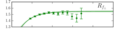
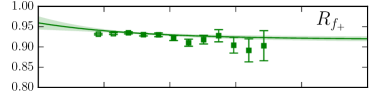
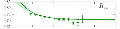
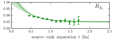
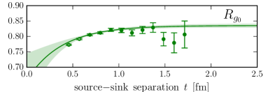
Figure 1: Lattice results from the CP ensemble for the ratios $R_{f}(|\mathbf{p}^{\prime}|,t)$, defined as in Eqs. (52-54) and (58-60) of Ref. Detmold:2015aaa , at $|\mathbf{p}^{\prime}|^{2}=4(2\pi/L)^{2}$. These ratios are equal to the ground-state form factors $f(|\mathbf{p}^{\prime}|)$ up to contamination from excited states that decays exponentially with $t$. The curves shown are correlated fits of the form $R_{f}(|\mathbf{p}^{\prime}|,t)=f(|\mathbf{p}^{\prime}|)+A_{f}(|\mathbf{p}^{\prime}|)\,e^{-\delta_{f}(|\mathbf{p}^{\prime}|)\,t}$, which includes the leading excited-state contributions. Data points at the smallest separations that are plotted with open symbols are excluded from the fits to suppress contamination from higher excited states; the values of $t_{\rm min}$ were chosen such that $\chi^{2}/{\rm d.o.f.}\leq 1$. The remaining systematic uncertainties due to higher excited states were estimated as the shifts in the fitted $f(|\mathbf{p}^{\prime}|)$ when further increasing $t_{\rm min}$ by one unit everywhere; these uncertainties were added in quadrature to the statistical uncertainties.

The $\Lambda_{c}\to\Lambda$ form factors are defined as in Eqs. (1) and (2) of Ref. Detmold:2016pkz (with $b$ replaced by $c$), and were extracted from ratios of three-point and two-point correlation functions using the same methods as in Detmold:2015aaa ; Detmold:2016pkz . This involves extrapolations to infinite source-sink separation to isolate the ground-state contributions, which are performed jointly for all data sets at matching $\Lambda$ momenta Detmold:2015aaa ; Detmold:2016pkz . These momenta, $|\mathbf{p}^{\prime}|^{2}$, were set to 1, 2, 3, and 4 times $(2\pi/L)^{2}$ on all data sets except CP. For the latter, the values 4, 8, 12, and 16 times $(2\pi/L)^{2}$ were used because $L=N_{s}a$ is twice as large. The ranges of source-sink separations were $t/a=4...15$ on the coarse lattices and $t/a=5...17$ on the fine lattices; full $\mathcal{O}(a)$-improvement of the currents was performed for all source-sink separations (instead of just a subset as in Refs. Detmold:2015aaa ; Detmold:2016pkz ). Examples for the ratios and $t\to\infty$ extrapolations are shown in Fig. 1.

The ground-state form factors obtained in this way for the different data sets and different discrete momenta are shown as the data points in Fig. 2. To obtain parametrizations of the form factors in the physical limit ($a=0$, $m_{\pi}=m_{\pi,{\rm phys}}$, $m_{\eta_{s}}=m_{\eta_{s},{\rm phys}}$), fits were then performed using $z$-expansions Bourrely:2008za modified with additional terms to describe the dependence on $a$, $m_{\pi}$, and $m_{\eta_{s}}$. In the physical limit, the fit functions reduce to the form

$$f(q^{2})=\frac{1}{1-q^{2}/(m_{\rm pole}^{f})^{2}}\sum_{n=0}^{n_{\rm max}}a_{n}^{f}[z(q^{2})]^{n},$$ (3)

where $z(q^{2})=\displaystyle\frac{\sqrt{t_{+}-q^{2}}-\sqrt{t_{+}-t_{0}}}{\sqrt{t_{+}-q^{2}}+\sqrt{t_{+}-t_{0}}}$ with $t_{0}=q^{2}_{\rm max}=(m_{\Lambda_{c}}-m_{\Lambda})^{2}$ and $t_{+}=(m_{D}+m_{K})^{2}$. The $D_{s}$ meson pole masses are $m_{\rm pole}^{f_{+},f_{\perp}}=2.112$ GeV, $m_{\rm pole}^{f_{0}}=2.318$ GeV, $m_{\rm pole}^{g_{+},g_{\perp}}=2.460$ GeV, $m_{\rm pole}^{g_{0}}=1.968$ GeV Olive:2016xmw , and to evaluate $t_{+}$, the masses $m_{D}=1.870\>{\rm GeV}$ and $m_{K}=494\>{\rm MeV}$ are used. Following Refs. Detmold:2015aaa ; Detmold:2016pkz , two separate fits were performed: a “nominal fit”, giving the central values and statistical uncertainties of the form factors, and a “higher-order fit”, used to compute systematic uncertainties according to Eqs. (50-56) of Ref. Detmold:2016pkz . The nominal fit had the same form as Eq. (36) of Ref. Detmold:2016pkz , but with $n_{\rm max}=2$ instead of $n_{\rm max}=1$ (no prior constraints on any parameters were used in the nominal fit). The higher-order fit had the same form as in Eq. (39) of Ref. Detmold:2016pkz , but with $n_{\rm max}=3$. In addition to the $z^{3}$ terms, this fit also includes terms of higher order in $a$, $m_{\pi}$, $m_{\eta_{s}}$, and was performed after modifying the data correlation matrix to include the uncertainties from the renormalization and $\mathcal{O}(a)$-improvement coefficients, from finite-volume effects (1.0%, rescaled from Ref. Detmold:2016pkz according to $e^{-{\rm min}[m_{\pi}L]}$), and from the missing isospin breaking/QED corrections (0.5%, 0.7%). The priors for the higher-order parameters were chosen as in Ref. Detmold:2016pkz , except that the coefficients $a_{2}^{f}$ were left unconstrained and the priors for $a_{3}^{f}$ were set to $0\pm 30$. The fit results for the parameters $a_{n}^{f}$ that describe the form factors in the physical limit are given in Table 4, and the form factors are plotted in Fig. 2. The lattice results do not significantly constrain the $z^{3}$ terms (note that $z_{\rm max}\approx 0.08$), so that their uncertainties are governed by the priors.

		Nominal fit		Higher-order fit
$a_{0}^{f_{\perp}}$		$\phantom{-}1.30\pm 0.06$		$\phantom{-}1.28\pm 0.07$
$a_{1}^{f_{\perp}}$		$-3.27\pm 1.18$		$-2.85\pm 1.34$
$a_{2}^{f_{\perp}}$		$\phantom{-}7.16\pm 11.6$		$\phantom{-}7.14\pm 12.2$
$a_{3}^{f_{\perp}}$				$-1.08\pm 30.0$
$a_{0}^{f_{+}}$		$\phantom{-}0.81\pm 0.03$		$\phantom{-}0.79\pm 0.04$
$a_{1}^{f_{+}}$		$-2.89\pm 0.52$		$-2.38\pm 0.61$
$a_{2}^{f_{+}}$		$\phantom{-}7.82\pm 4.53$		$\phantom{-}6.64\pm 6.07$
$a_{3}^{f_{+}}$				$-1.08\pm 29.8$
$a_{0}^{f_{0}}$		$\phantom{-}0.77\pm 0.02$		$\phantom{-}0.76\pm 0.03$
$a_{1}^{f_{0}}$		$-2.24\pm 0.51$		$-1.77\pm 0.58$
$a_{2}^{f_{0}}$		$\phantom{-}5.38\pm 4.80$		$\phantom{-}4.93\pm 6.28$
$a_{3}^{f_{0}}$				$-0.26\pm 29.8$
$a_{0}^{g_{\perp},g_{+}}$		$\phantom{-}0.68\pm 0.02$		$\phantom{-}0.67\pm 0.02$
$a_{1}^{g_{\perp}}$		$-1.91\pm 0.35$		$-1.73\pm 0.54$
$a_{2}^{g_{\perp}}$		$\phantom{-}6.24\pm 4.89$		$\phantom{-}5.97\pm 6.64$
$a_{3}^{g_{\perp}}$				$-1.68\pm 29.8$
$a_{1}^{g_{+}}$		$-2.44\pm 0.25$		$-2.22\pm 0.35$
$a_{2}^{g_{+}}$		$\phantom{-}13.7\pm 2.15$		$\phantom{-}12.1\pm 4.43$
$a_{3}^{g_{+}}$				$\phantom{-}12.9\pm 29.2$
$a_{0}^{g_{0}}$		$\phantom{-}0.71\pm 0.03$		$\phantom{-}0.72\pm 0.04$
$a_{1}^{g_{0}}$		$-2.86\pm 0.44$		$-2.80\pm 0.53$
$a_{2}^{g_{0}}$		$\phantom{-}11.8\pm 2.47$		$\phantom{-}11.7\pm 4.74$
$a_{3}^{g_{0}}$				$\phantom{-}1.35\pm 29.4$

Table 4: Results for the $z$-expansion parameters describing the form factors in the physical limit. Files containing the parameter values with more digits and the full covariance matrices are provided as supplemental material supplementalmaterial .

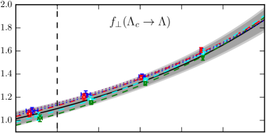
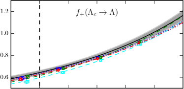
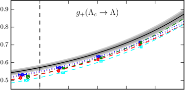
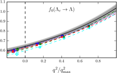
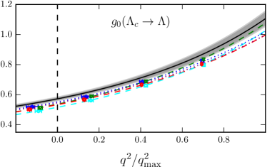
Figure 2: Lattice QCD results for the $\Lambda_{c}\to\Lambda$ form factors, along with the modified $z$-expansion fits evaluated at the lattice parameters (dashed and dotted lines) and in the physical limit (solid lines, with statistical and total uncertainties indicated by the inner and outer bands).

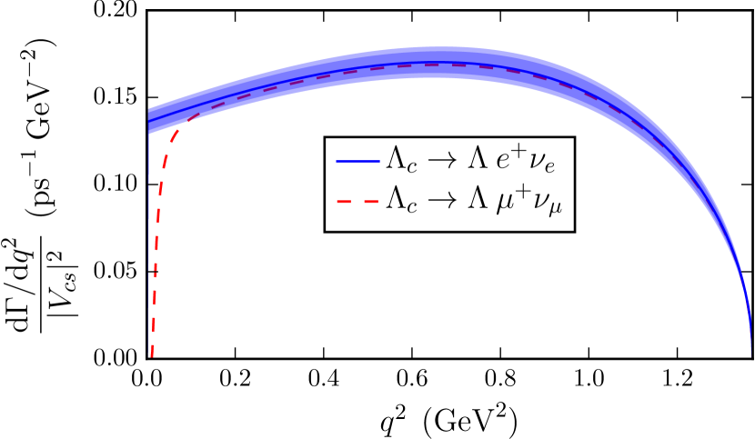
Figure 3: Predictions for the $\Lambda_{c}\to\Lambda\ell^{+}\nu_{\ell}$ differential decay rates (divided by $|V_{cs}|^{2}$) in the Standard Model. For clarity, the uncertainties are shown only for $\ell=e$; the inner and outer bands correspond to the statistical and total uncertainties.

The resulting Standard-Model predictions for the $\Lambda_{c}\to\Lambda\ell^{+}\nu_{\ell}$ differential decay rates, without the factor of $|V_{cs}|^{2}$, are shown in Fig. 3. The $q^{2}$-integrated rates are

$$\frac{\Gamma(\Lambda_{c}\to\Lambda\ell^{+}\nu_{\ell})}{|V_{cs}|^{2}}=\left\{\begin{array}[]{ll}0.2007(71)(74)\>{\rm ps}^{-1},&\ell=e,\\ 0.1945(69)(72)\>{\rm ps}^{-1},&\ell=\mu,\end{array}\right.$$ (4)

where the two uncertainties are from the statistical and total systematic uncertainties in the form factors. Using the world average of $\Lambda_{c}$ lifetime measurements, $\tau_{\Lambda_{c}}=0.200(6)\>{\rm ps}$ Olive:2016xmw , and $|V_{cs}|=0.97344(15)$ from a CKM unitarity global fit UTfit then yields the branching fractions

$$\mathcal{B}(\Lambda_{c}\to\Lambda\ell^{+}\nu_{\ell})=\left\{\begin{array}[]{ll}0.0380(19)_{\rm LQCD}(11)_{\tau_{\Lambda_{c}}},&\ell=e,\\ 0.0369(19)_{\rm LQCD}(11)_{\tau_{\Lambda_{c}}},&\ell=\mu,\end{array}\right.$$ (5)

where the uncertainties marked “LQCD” are the total form factor uncertainties from the lattice calculation. These results are consistent with, and two times more precise than, the BESIII measurements shown in Eq. (2). This is a valuable check of the lattice methods which were also used in Refs. Aaij:2015bfa ; Meinel:2016grj ; Detmold:2015aaa ; Detmold:2016pkz .

Combining instead the BESIII measurements (2) and $\tau_{\Lambda_{c}}=0.200(6)\>{\rm ps}$ with the results in Eq. (4) to determine $|V_{cs}|$ from $\Lambda_{c}\to\Lambda\ell^{+}\nu_{\ell}$ gives

$$|V_{cs}|=\left\{\begin{array}[]{ll}0.951(24)_{\rm LQCD}(14)_{\tau_{\Lambda_{c}}}(56)_{\mathcal{B}},&\ell=e,\\ 0.947(24)_{\rm LQCD}(14)_{\tau_{\Lambda_{c}}}(72)_{\mathcal{B}},&\ell=\mu,\\ 0.949(24)_{\rm LQCD}(14)_{\tau_{\Lambda_{c}}}(49)_{\mathcal{B}},&\ell=e,\mu,\end{array}\right.$$ (6)

where the last line is the correlated average over $\ell=e,\mu$. This is the first determination of $|V_{cs}|$ from baryonic decays. The result is consistent with CKM unitarity, and the uncertainty can be reduced further with more precise measurements of the $\Lambda_{c}\to\Lambda\ell^{+}\nu_{\ell}$ branching fractions.

- (1) LHCb Collaboration, R. Aaij et al., “Determination of the quark coupling strength using baryonic decays,” Nature Phys. 11 (2015) 743–747, arXiv:1504.01568 [hep-ex].
- (2) S. Meinel and D. van Dyk, “Using data within a Bayesian analysis of decays,” Phys. Rev. D94 no. 1, (2016) 013007, arXiv:1603.02974 [hep-ph].
- (3) W. Detmold, C. Lehner, and S. Meinel, “ and form factors from lattice QCD with relativistic heavy quarks,” Phys. Rev. D92 no. 3, (2015) 034503, arXiv:1503.01421 [hep-lat].
- (4) W. Detmold and S. Meinel, “ form factors, differential branching fraction, and angular observables from lattice QCD with relativistic quarks,” Phys. Rev. D93 no. 7, (2016) 074501, arXiv:1602.01399 [hep-lat].
- (5) Fermilab Lattice, MILC Collaboration, A. Bazavov et al., “Charmed and light pseudoscalar meson decay constants from four-flavor lattice QCD with physical light quarks,” Phys. Rev. D90 no. 7, (2014) 074509, arXiv:1407.3772 [hep-lat].
- (6) S. Aoki et al., “Review of lattice results concerning low-energy particle physics,” arXiv:1607.00299 [hep-lat].
- (7) HPQCD Collaboration, H. Na, C. T. H. Davies, E. Follana, G. P. Lepage, and J. Shigemitsu, “The Semileptonic Decay Scalar Form Factor and from Lattice QCD,” Phys. Rev. D82 (2010) 114506, arXiv:1008.4562 [hep-lat].
- (8) UTfit Collaboration, “Standard model fit results: Winter 2016.” http://www.utfit.org/UTfit/ResultsWinter2016.
- (9) S. Fajfer, I. Nisandzic, and U. Rojec, “Discerning new physics in charm meson leptonic and semileptonic decays,” Phys. Rev. D91 no. 9, (2015) 094009, arXiv:1502.07488 [hep-ph].
- (10) J. L. Rosner, “Prospects for improved branching fractions,” Phys. Rev. D86 (2012) 014017, arXiv:1205.4964 [hep-ph].
- (11) BESIII Collaboration, M. Ablikim et al., “Measurement of the absolute branching fraction for ,” Phys. Rev. Lett. 115 no. 22, (2015) 221805, arXiv:1510.02610 [hep-ex].
- (12) BESIII Collaboration, M. Ablikim et al., “Measurement of the Absolute Branching Fraction for ,” Phys. Lett. B767 (2017) 42–47, arXiv:1611.04382 [hep-ex].
- (13) A. J. Buras, “Semileptonic Decays of Charmed Baryons,” Nucl. Phys. B109 (1976) 373–396.
- (14) M. B. Gavela, “Semileptonic Decays of Charmed Particles,” Phys. Lett. B83 (1979) 367–370.
- (15) M. Avila-Aoki, A. Garcia, R. Huerta, and R. Perez-Marcial, “Predictions for Semileptonic Decays of Charm Baryons. 1. Symmetry Limit,” Phys. Rev. D40 (1989) 2944.
- (16) R. Perez-Marcial, R. Huerta, A. Garcia, and M. Avila-Aoki, “Predictions for Semileptonic Decays of Charm Baryons. 2. Nonrelativistic and MIT Bag Quark Models,” Phys. Rev. D40 (1989) 2955. [Erratum: Phys. Rev.D44,2203(1991)].
- (17) F. Hussain and J. G. Krner, “Semileptonic charm baryon decays in the relativistic spectator quark model,” Z. Phys. C51 (1991) 607–614.
- (18) R. L. Singleton, “Semileptonic baryon decays with a heavy quark,” Phys. Rev. D43 (1991) 2939–2950.
- (19) G. V. Efimov, M. A. Ivanov, and V. E. Lyubovitskij, “Predictions for semileptonic decay rates of charmed baryons in the quark confinement model,” Z. Phys. C52 (1991) 149–158.
- (20) A. Garcia and R. Huerta, “Semileptonic decays of charmed baryons,” Phys. Rev. D45 (1992) 3266–3267.
- (21) H.-Y. Cheng and B. Tseng, “ corrections to baryonic form-factors in the quark model,” Phys. Rev. D53 (1996) 1457, arXiv:hep-ph/9502391 [hep-ph]. [Erratum: Phys. Rev.D55,1697(1997)].
- (22) M. A. Ivanov, V. E. Lyubovitskij, J. G. Krner, and P. Kroll, “Heavy baryon transitions in a relativistic three quark model,” Phys. Rev. D56 (1997) 348–364, arXiv:hep-ph/9612463 [hep-ph].
- (23) H. G. Dosch, E. Ferreira, M. Nielsen, and R. Rosenfeld, “Evidence from QCD sum rules for large violation of heavy quark symmetry in semileptonic decay,” Phys. Lett. B431 (1998) 173–178, arXiv:hep-ph/9712350 [hep-ph].
- (24) C. W. Luo, “Heavy to light baryon weak form-factors in the light cone constituent quark model,” Eur. Phys. J. C1 (1998) 235–241.
- (25) R. S. Marques de Carvalho, F. S. Navarra, M. Nielsen, E. Ferreira, and H. G. Dosch, “Form-factors and decay rates for heavy semileptonic decays from QCD sum rules,” Phys. Rev. D60 (1999) 034009, arXiv:hep-ph/9903326 [hep-ph].
- (26) M. Pervin, W. Roberts, and S. Capstick, “Semileptonic decays of heavy baryons in a quark model,” Phys. Rev. C72 (2005) 035201, arXiv:nucl-th/0503030 [nucl-th].
- (27) Y.-L. Liu, M.-Q. Huang, and D.-W. Wang, “Improved analysis on the semi-leptonic decay from QCD light-cone sum rules,” Phys. Rev. D80 (2009) 074011, arXiv:0910.1160 [hep-ph].
- (28) T. Gutsche, M. A. Ivanov, J. G. Krner, V. E. Lyubovitskij, and P. Santorelli, “Semileptonic decays in the covariant quark model and comparison with the new absolute branching fraction measurements of Belle and BESIII,” Phys. Rev. D93 no. 3, (2016) 034008, arXiv:1512.02168 [hep-ph].
- (29) R. N. Faustov and V. O. Galkin, “Semileptonic decays of baryons in the relativistic quark model,” Eur. Phys. J. C76 no. 11, (2016) 628, arXiv:1610.00957 [hep-ph].
- (30) RBC, UKQCD Collaboration, T. Blum et al., “Domain wall QCD with physical quark masses,” Phys. Rev. D93 no. 7, (2016) 074505, arXiv:1411.7017 [hep-lat].
- (31) RBC, UKQCD Collaboration, Y. Aoki et al., “Continuum Limit Physics from 2+1 Flavor Domain Wall QCD,” Phys.Rev. D83 (2011) 074508, arXiv:1011.0892 [hep-lat].
- (32) S. Meinel, “Bottomonium spectrum at order from domain-wall lattice QCD: Precise results for hyperfine splittings,” Phys. Rev. D82 (2010) 114502, arXiv:1007.3966 [hep-lat].
- (33) HPQCD Collaboration, C. T. H. Davies, E. Follana, I. D. Kendall, G. P. Lepage, and C. McNeile, “Precise determination of the lattice spacing in full lattice QCD,” Phys. Rev. D81 (2010) 034506, arXiv:0910.1229 [hep-lat].
- (34) HPQCD Collaboration, R. J. Dowdall et al., “The Upsilon spectrum and the determination of the lattice spacing from lattice QCD including charm quarks in the sea,” Phys. Rev. D85 (2012) 054509, arXiv:1110.6887 [hep-lat].
- (35) E. Shintani, R. Arthur, T. Blum, T. Izubuchi, C. Jung, and C. Lehner, “Covariant approximation averaging,” Phys. Rev. D91 no. 11, (2015) 114511, arXiv:1402.0244 [hep-lat].
- (36) Z. S. Brown, W. Detmold, S. Meinel, and K. Orginos, “Charmed bottom baryon spectroscopy from lattice QCD,” Phys. Rev. D90 no. 9, (2014) 094507, arXiv:1409.0497 [hep-lat].
- (37) Particle Data Group Collaboration, C. Patrignani et al., “Review of Particle Physics,” Chin. Phys. C40 no. 10, (2016) 100001.
- (38) S. Hashimoto, A. X. El-Khadra, A. S. Kronfeld, P. B. Mackenzie, S. M. Ryan, et al., “Lattice QCD calculation of decay form-factors at zero recoil,” Phys.Rev. D61 (1999) 014502, arXiv:hep-ph/9906376 [hep-ph].
- (39) A. X. El-Khadra, A. S. Kronfeld, P. B. Mackenzie, S. M. Ryan, and J. N. Simone, “The Semileptonic decays and from lattice QCD,” Phys.Rev. D64 (2001) 014502, arXiv:hep-ph/0101023 [hep-ph].
- (40) C. Lehner, “Automated lattice perturbation theory and relativistic heavy quarks in the Columbia formulation,” PoS LATTICE2012 (2012) 126, arXiv:1211.4013 [hep-lat].
- (41) C. Lehner. Private communication, 2016.
- (42) C. Bourrely, I. Caprini, and L. Lellouch, “Model-independent description of decays and a determination of ,” Phys.Rev. D79 (2009) 013008, arXiv:0807.2722 [hep-ph].
- (43) See https://arxiv.org/src/1611.09696/anc for files containing the form factor parameter values and covariances.
- (44) SciDAC, LHPC, UKQCD Collaboration, R. G. Edwards and B. Joo, “The Chroma software system for lattice QCD,” Nucl.Phys.Proc.Suppl. 140 (2005) 832, arXiv:hep-lat/0409003 [hep-lat].
- (45) https://usqcd.lns.mit.edu/w/index.php/QLUA.
- (46) T. Kurth, A. Pochinsky, A. Sarje, S. Syritsyn, and A. Walker-Loud, “High-Performance I/O: HDF5 for Lattice QCD,” PoS LATTICE2014 (2015) 045, arXiv:1501.06992 [hep-lat].