Investigation of thermalization in giant-spin models by different Lindblad schemes

Abstract

The theoretical understanding of time-dependence in magnetic quantum systems is of great importance in particular for cases where a unitary time evolution is accompanied by relaxation processes. A key example is given by the dynamics of single-molecule magnets where quantum tunneling of the magnetization competes with thermal relaxation over the anisotropy barrier. In this article we investigate how good a Lindblad approach describes the relaxation in giant spin models and how the result depends on the employed operator that transmits the action of the thermal bath.

1 Introduction

Single-molecule magnets (SMM) show two interesting phenomena: slow relaxation and quantum tunneling of the magnetization [1, 2, 3]. Very often both processes are modeled independently of each other. Relaxation is accounted for by rate equations, see e.g. Refs. [4, 5, 6, 7, 8], whereas quantum tunneling is described by a unitary time evolution [5], e.g. in terms of the von Neumann equation. Only a few approaches have been undertaken in order obtain a combined description.

In this article we investigate a master-equation approach that rests on the use of Lindblad terms [9, 10, 11, 12, 13, 14, 15, 16, 17]. Although such an approach lacks memory effects [18, 11] it constitutes a minimal feasible description of a time evolution that combines coherent and incoherent parts. Besides application for magnetization dynamics such a description is of paramount importance for the investigation of quantum computing schemes and their robustness [17].

The Lindblad terms in the master equation usually summarize the effects of the various relaxation processes [19] in terms of transition operators acting between the eigenstates of the investigated quantum spin system. Although it might in principle be possible to derive such terms from basic principles [6, 20], the employed functional form of these terms leaves room to tweak unknown parameters [16]. In the following we introduce some of the common approaches and investigate how the resulting magnetization dynamics depends on the parameterization. Our impression is that this dependence is in general non-negligible and in particular for the evaluation of the ac magnetization rather strong, so that results from such simulations have to be interpreted with great care.

The article is organized as follows. In section 2 we introduce the model. Sections 3 and 4 deal with dc and ac magnetization, respectively. Our results are summarized in section 5.

2 Model and numerical procedures

For the investigations throughout this article we employ the following giant spin Hamiltonian [21]

$$\!\hbox{}\mathop{\vphantom{H}\smash{H}}\limits_{\sim}\hbox{}\! = D\;\!\hbox{}\mathop{\vphantom{S}\smash{S}}\limits_{\sim}\!{}_{z}^{2}+E\;\left(\!\hbox{}\mathop{\vphantom{S}\smash{S}}\limits_{\sim}\!{}_{x}^{2}-\!\hbox{}\mathop{\vphantom{S}\smash{S}}\limits_{\sim}\!{}_{y}^{2}\right)+g\,\mu_{B}\,\vec{B}(t)\cdot\!\hbox{}\mathop{\vphantom{\vec{S}}\smash{\vec{S}}}\limits_{\sim}\hbox{}\!\ ,$$ (1)

with specific values of $D=-1\text{~{}K}$, $E=0.1\text{~{}K}$ and $g=2$ used in the numerical simulations. Such Hamiltonians describe SMMs with an easy axis anisotropy of strength $D<0$.

For the time evolution of the density matrix we employ [16]

$$\frac{d}{dt}\;\!\hbox{}\mathop{\vphantom{\rho}\smash{\rho}}\limits_{\sim}\hbox{}\!\left(t\right) = -i\left[\!\hbox{}\mathop{\vphantom{H}\smash{H}}\limits_{\sim}\hbox{}\!,\!\hbox{}\mathop{\vphantom{\rho}\smash{\rho}}\limits_{\sim}\hbox{}\!\left(t\right)\right]-\lambda\left(\left[\!\hbox{}\mathop{\vphantom{X}\smash{X}}\limits_{\sim}\hbox{}\!,\!\hbox{}\mathop{\vphantom{R}\smash{R}}\limits_{\sim}\hbox{}\!\!\hbox{}\mathop{\vphantom{\rho}\smash{\rho}}\limits_{\sim}\hbox{}\!\left(t\right)\right]+\left[\!\hbox{}\mathop{\vphantom{X}\smash{X}}\limits_{\sim}\hbox{}\!,\!\hbox{}\mathop{\vphantom{R}\smash{R}}\limits_{\sim}\hbox{}\!\!\hbox{}\mathop{\vphantom{\rho}\smash{\rho}}\limits_{\sim}\hbox{}\!\left(t\right)\right]^{\dagger}\right)\ ,$$ (2)

with

$$\left\langle k\right|\!\hbox{}\mathop{\vphantom{R}\smash{R}}\limits_{\sim}\hbox{}\!\left|n\right\rangle = \frac{I\left(E_{k}-E_{n}\right)-I\left(E_{n}-E_{k}\right)}{e^{\beta\left(E_{k}-E_{n}\right)}-1}\left\langle k\right|\!\hbox{}\mathop{\vphantom{X}\smash{X}}\limits_{\sim}\hbox{}\!\left|n\right\rangle\ ,$$ (3)

where $\left|k\right\rangle$ and $\left|n\right\rangle$ are eigenvectors of the Hamiltonian with corresponding eigenvalues $E_{k}$ and $E_{n}$. In such an approach it is implicitly assumed that the coupling to the heat bath is realized by phonons [13], whose spectral density is denoted by $I\left(\omega\right)$

$$I\left(E_{k}-E_{n}\right) = I_{0}\cdot\left(E_{k}-E_{n}\right)$$ (4)

with $I_{0}=1$. The related transition operator $\!\hbox{}\mathop{\vphantom{X}\smash{X}}\limits_{\sim}\hbox{}\!$ mediates the action of the heat bath onto the giant spin of (1). We investigate several typical choices for this operator. For one choice of transition operators we use those suggested in [13]:

$$\!\hbox{}\mathop{\vphantom{X}\smash{X}}\limits_{\sim}\!{}_{1} = \!\hbox{}\mathop{\vphantom{S}\smash{S}}\limits_{\sim}\!{}_{x}\ ,$$ (5)

$$\!\hbox{}\mathop{\vphantom{X}\smash{X}}\limits_{\sim}\!{}_{2} = \frac{1}{2}\left(\!\hbox{}\mathop{\vphantom{S}\smash{S}}\limits_{\sim}\!{}_{x}+\!\hbox{}\mathop{\vphantom{S}\smash{S}}\limits_{\sim}\!{}_{z}\right)\ .$$ (6)

These two operators generate transitions among eigenstates of Hamiltonian (1) with $\Delta m=0,\pm 1$. We investigate as well another operator

$$\!\hbox{}\mathop{\vphantom{X}\smash{X}}\limits_{\sim}\!{}_{3} = \frac{4}{5}\!\hbox{}\mathop{\vphantom{S}\smash{S}}\limits_{\sim}\!{}_{x}+\frac{1}{5}\!\hbox{}\mathop{\vphantom{S}\smash{S}}\limits_{\sim}\!{}_{x}^{2}\ ,$$ (7)

that via its $\!\hbox{}\mathop{\vphantom{S}\smash{S}}\limits_{\sim}\!{}_{x}^{2}$ contribution effectively takes also two-phonon processes with $\Delta m=\pm 2$ into account.

The influence of a spin bath, e.g. nuclear spins in the sample, is not taken into account by this approach [22].

3 Magnetization dynamics: tunneling and hysteresis

In order to investigate the magnetization dynamics the magnetic field in $z$-direction is swept from $-2$ to $+2\text{~{}T}$ with a sweep-rate of $0.625\text{~{}T/ns}$. For the simulations the sweep rate has to assume such high values since otherwise simulations covering the complete magnetization process are not feasible [13]. This problem is caused by the intrinsic energy scales (GHz frequencies) and it is common to many problems in simulation science. The gaps at the avoided level crossings are adapted accordingly by choosing a constant field of $B_{x}=0.2\text{~{}T}$ in $x$-direction.

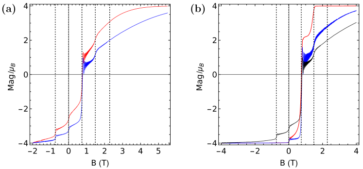
Figure 1: Magnetization in $z$-direction: The vertical dashed lines correspond to magnetic field strengths where resonant tunneling is possible. (a) $T=2$ K and $\lambda=10^{-4}$ with $\!\hbox{}\mathop{\vphantom{X}\smash{X}}\limits_{\sim}\!{}_{1}$ (red) and $\!\hbox{}\mathop{\vphantom{X}\smash{X}}\limits_{\sim}\!{}_{2}$ (blue). (b) Magnetization curve with $\!\hbox{}\mathop{\vphantom{X}\smash{X}}\limits_{\sim}\!{}_{2}$ and $T=0.01$ K, $\lambda=10^{-2}$ (red), $T=0.01$ K, $\lambda=10^{-4}$ (blue), $T=2$ K, $\lambda=10^{-4}$ (black).

Figure 1 shows the step-wise behavior of the magnetization in $z$-direction for the first two choices of $\!\hbox{}\mathop{\vphantom{X}\smash{X}}\limits_{\sim}\hbox{}\!$. All magnetization steps appear at magnetic field strengths where resonant tunneling is possible (as indicated by the vertical dashed lines in Figure 1). As already predicted in [13] one can see in figure 2 (a) that the relaxation with $\!\hbox{}\mathop{\vphantom{X}\smash{X}}\limits_{\sim}\hbox{}\!=\!\hbox{}\mathop{\vphantom{X_{1}}\smash{X_{1}}}\limits_{\sim}\hbox{}\!$ is more efficient than the one with $\!\hbox{}\mathop{\vphantom{X}\smash{X}}\limits_{\sim}\hbox{}\!=\!\hbox{}\mathop{\vphantom{X}\smash{X}}\limits_{\sim}\!{}_{2}$ in the sense that the magnetization reaches saturation much faster. This is very likely due to the factor $\frac{1}{2}$ in $\!\hbox{}\mathop{\vphantom{X}\smash{X}}\limits_{\sim}\!{}_{2}$, which reduces the transition rates induced by $\!\hbox{}\mathop{\vphantom{S}\smash{S}}\limits_{\sim}\!{}_{x}$. Beside this difference in efficiency both curves look qualitatively similar.

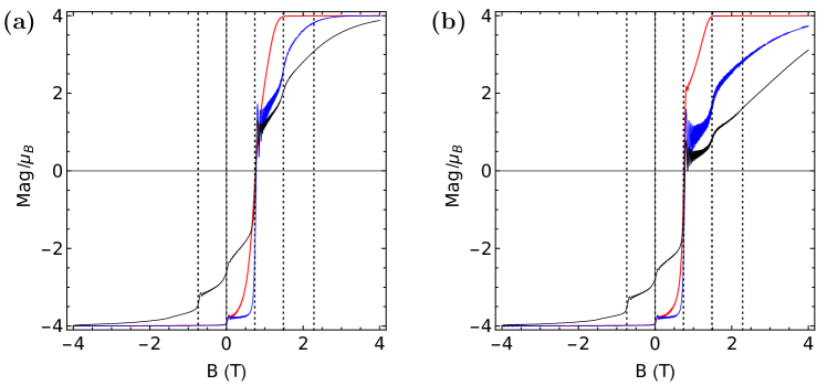
Figure 2: Magnetization in $z$-direction: The vertical dashed lines correspond to magnetic field strengths where resonant tunneling is possible. (a) Magnetization curve with $\!\hbox{}\mathop{\vphantom{X}\smash{X}}\limits_{\sim}\!{}_{1}$ and $T=0.01$ K, $\lambda=10^{-2}$ (red), $T=0.01$ K, $\lambda=10^{-4}$ (blue), $T=2$ K, $\lambda=10^{-4}$ (black). (b) Magnetization curve with $\!\hbox{}\mathop{\vphantom{X}\smash{X}}\limits_{\sim}\!{}_{3}$ and $T=0.01$ K, $\lambda=10^{-2}$ (red), $T=0.01$ K, $\lambda=10^{-4}$ (blue), $T=2$ K, $\lambda=10^{-4}$ (black).

Figure 1 (b) and figure 2 (a) & (b) show magnetization curves for all three transition operators at different temperatures and with different coupling constants $\lambda$. In every case the curves calculated at $T=2$ K (black curves in figs. 1 (b) and 2) show steps, that can only occur because the involved level-crossings are already thermally occupied. For $\!\hbox{}\mathop{\vphantom{X}\smash{X}}\limits_{\sim}\hbox{}\!=\!\hbox{}\mathop{\vphantom{X}\smash{X}}\limits_{\sim}\!{}_{1}$ and $\!\hbox{}\mathop{\vphantom{X}\smash{X}}\limits_{\sim}\!{}_{3}$ these steps have qualitatively nearly the same step size, only in the curve with $\!\hbox{}\mathop{\vphantom{X}\smash{X}}\limits_{\sim}\hbox{}\!=\!\hbox{}\mathop{\vphantom{X}\smash{X}}\limits_{\sim}\!{}_{2}$ they are smaller, most likely due to the factor $\frac{1}{2}$ in $\!\hbox{}\mathop{\vphantom{X}\smash{X}}\limits_{\sim}\!{}_{2}$. The thermal relaxation after the last step is also different. Qualitatively the efficiency is increasing with the amount of $\!\hbox{}\mathop{\vphantom{S}\smash{S}}\limits_{\sim}\!{}_{x}$ in the relaxation operator. The behavior at $T=0.01$ K and $\lambda=10^{-2}$ (red curves in figs. 1 (b) and 2) also shows differences in the efficiency. The curve with $\!\hbox{}\mathop{\vphantom{X}\smash{X}}\limits_{\sim}\hbox{}\!=\!\hbox{}\mathop{\vphantom{X}\smash{X}}\limits_{\sim}\!{}_{1}$ is again the most efficient one. Only two steps are needed to end up at the saturation magnetization. Both other curves show a third step. The visibility of this step increases with the decreasing amount of $\!\hbox{}\mathop{\vphantom{S}\smash{S}}\limits_{\sim}\!{}_{x}$ in the transition operator.

As expected, a stronger coupling to the bath, i.e. a larger parameter $\lambda$ leads to a quicker relaxation with reduced quantum oscillations (compare red and blue curves in figures 1 (b) and 2).

4 Magnetization dynamics: AC susceptibility and relaxation times

AC susceptometry is a powerful experimental tool to get access to the relaxation processes. Theoretically ac susceptibilities are complicated non-equilibrium quantities since they involve the influence of, and thus the coupling to the bath. It is thus expected that properties of the bath and the coupling will in general influence ac measurements [22].

In our simulations we apply a magnetic ac field of the form

$$B_{z}\left(t\right) = B_{0}\cdot\cos\left(\omega t\right)$$ (8)

in $z$-direction. It is important that the amplitude $B_{0}$ is small enough, so that the magnetization of the system does not reach its saturation value. We choose $B_{0}=0.001\text{ T}$. In the steady state the magnetization of the system is given by [23]:

$$M\left(t\right) = \left(\chi^{{}^{\prime}}\cos\left(\omega t\right)+\chi^{{}^{\prime\prime}}\sin\left(\omega t\right)\right)B_{0}\>,$$ (9)

where $\chi^{{}^{\prime}}$ and $\chi^{{}^{\prime\prime}}$ are the real and imaginary part of the magnetic susceptibility. Both can be calculated from $M\left(t\right)$ via integration over one period. The relaxation time $\tau$ can then be found as

$$\tau = \frac{1}{\omega_{\text{max}}}$$ (10)

with $\omega_{\text{max}}$ the frequency of the maximum of $\chi^{{}^{\prime\prime}}$. The great advantage of this method is that it is possible to calculate the relaxation times in the temperature regime where quantum tunneling is the dominant process and the relaxation time becomes temperature independent.

In our simulations of the ac susceptibility we set the coupling to the phonon heat bath $\lambda=1$. We want to stress here, that the observed behavior is also present with much smaller coupling constants. Smaller coupling constants only lead to a shift of the temperature at which quantum tunneling becomes the dominant process.

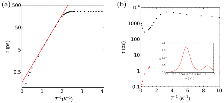
Figure 3: (a) Temperature dependent relaxation times of the magnetization in z-direction (black dots) for the $S=2$ system with $\!\hbox{}\mathop{\vphantom{X}\smash{X}}\limits_{\sim}\!{}_{1}$. Fitted Arrhenius law with $\tau_{0}=0.171$ ps and $DS^{2}=3.48$ (red line). (b) Temperature dependent dominant relaxation time of the magnetization in $z$-direction (black dots) for the $S=2$ system with $\!\hbox{}\mathop{\vphantom{X}\smash{X}}\limits_{\sim}\!{}_{2}$. Red dots: second relaxation time, which disappears below $T=0.9$ K. Please note the different scales for $\tau$. The inset shows one example of $\chi^{{}^{\prime\prime}}$ vs. $\omega$ where the two peaks belonging to the dominant and second relaxation times are clearly visible.

Figure 3 (a) shows the calculated relaxation time for the $S=2$ system with $\!\hbox{}\mathop{\vphantom{X}\smash{X}}\limits_{\sim}\hbox{}\!=\!\hbox{}\mathop{\vphantom{X}\smash{X}}\limits_{\sim}\!{}_{1}$. For temperatures between $0.5\text{ K}$ and $1\text{ K}$ the relaxation times are well described by the Arrhenius law

$$\tau = \tau_{0}\cdot\exp\left[\frac{\Delta}{T}\right]$$ (11)

with fitted parameters $\tau_{0}=0.17144\pm 0.008546\text{ ps}$ and $\Delta=3.48091\pm 0.03101\text{ K}$. This is in quite good agreement with the theoretical value of $\Delta_{\text{th}}=DS^{2}=4\text{ K}$. Below $0.5\text{ K}$ the resonant tunneling becomes the dominant process and the relaxation time becomes independent of temperature [24].

Figure 3 (b) shows the temperature dependent relaxation times for the $S=2$ system with $\!\hbox{}\mathop{\vphantom{X}\smash{X}}\limits_{\sim}\hbox{}\!=\!\hbox{}\mathop{\vphantom{X}\smash{X}}\limits_{\sim}\!{}_{2}$. Here we find for temperatures larger than $0.9\text{ K}$ a second relaxation time. Below $0.9\text{ K}$ it is no longer visible because its peak in $\chi^{{}^{\prime\prime}}$ is masked by the peak belonging to the dominant relaxation time. The dominant relaxation time itself shows an unphysical behavior: at higher temperatures it is again increasing with increasing temperature. This is in contradiction to experimentally measured data as well as to the whole idea of activated behavior. We verified that this observation is not an artifact of the relatively high value of the coupling constant $\lambda$. The observed unphysical behavior is also present with much smaller values of $\lambda$, but smaller values shift the strange behavior to higher temperatures. We also noticed that the unphysical behavior is present for any amount of $\!\hbox{}\mathop{\vphantom{S}\smash{S}}\limits_{\sim}\!{}_{z}$ in the transition operator $\!\hbox{}\mathop{\vphantom{X}\smash{X}}\limits_{\sim}\hbox{}\!$. We thus conjecture that the unphysical behavior is solely due to the presence of $\!\hbox{}\mathop{\vphantom{S}\smash{S}}\limits_{\sim}\!{}_{z}$ in the transition operator. Its use as a transition operator thus appears questionable, although other observables such as the magnetization investigated in section 3 do not show (obvious) unphysical behavior.

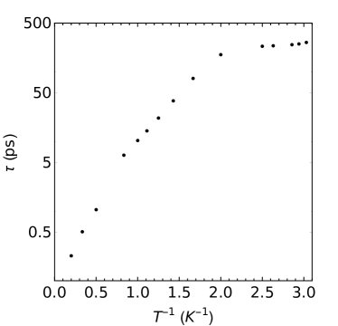
Figure 4: Temperature dependent relaxation time of the magnetization in $z$-direction (black dots) for the $S=2$ system with $\!\hbox{}\mathop{\vphantom{X}\smash{X}}\limits_{\sim}\!{}_{3}$.

In order to investigate the influence of absorption and emission of phonons with $\Delta m=\pm 2$ we also calculated the relaxation times for the $S=2$ system with $\!\hbox{}\mathop{\vphantom{X}\smash{X}}\limits_{\sim}\hbox{}\!=\!\hbox{}\mathop{\vphantom{X}\smash{X}}\limits_{\sim}\!{}_{3}$. The results are shown in figure 4. Firstly, $\!\hbox{}\mathop{\vphantom{X}\smash{X}}\limits_{\sim}\hbox{}\!=\!\hbox{}\mathop{\vphantom{X}\smash{X}}\limits_{\sim}\!{}_{3}$ does not lead to (obvious) unphysical behavior. Secondly, it is impossible to fit the curve with one standard Arrhenius law (11). At least two of them would be necessary, one above and one below $T=1$ K. Qualitatively the relaxation times in the regime of resonant tunneling, where the relaxation time becomes independent of the temperature, are nearly the same for $\!\hbox{}\mathop{\vphantom{X}\smash{X}}\limits_{\sim}\hbox{}\!=\!\hbox{}\mathop{\vphantom{X}\smash{X}}\limits_{\sim}\!{}_{3}$ and $\!\hbox{}\mathop{\vphantom{X}\smash{X}}\limits_{\sim}\hbox{}\!=\!\hbox{}\mathop{\vphantom{X}\smash{X}}\limits_{\sim}\!{}_{1}$. This is not an effect of the large amount of $\!\hbox{}\mathop{\vphantom{S}\smash{S}}\limits_{\sim}\!{}_{x}$ in $\!\hbox{}\mathop{\vphantom{X}\smash{X}}\limits_{\sim}\!{}_{3}$. If $\!\hbox{}\mathop{\vphantom{X}\smash{X}}\limits_{\sim}\hbox{}\!=\!\hbox{}\mathop{\vphantom{S}\smash{S}}\limits_{\sim}\!{}_{x}^{2}$ is chosen (not shown here) the same behavior occurs.

5 Summary

In this article we report on numerical studies of the quantum dynamics of giant spin models by means of the Lindblad scheme. Such equations of motion for the density matrix allow to treat unitary as well as relaxation dynamics together with the prospect of simulating really large spin systems [25, 26] in the future.

Our concern was to investigate the influence of the employed transition operators on non-equilibrium observables such as the magnetization. We demonstrated that it is possible to evaluate magnetization processes as well as ac susceptibilities. From the latter relaxation times can be extracted, and their dependence on frequency and temperature can be studied. This provides an additional and very valuable tool to better understand the experimental ac data.

Unfortunately, the method is limited by two factors. A useful comparison between theory and experiment needs a detailed knowledge of the transition operator $\!\hbox{}\mathop{\vphantom{X}\smash{X}}\limits_{\sim}\hbox{}\!$, upon which non-equilibrium observables depend strongly as we showed in this work. The second limitation is common to all kinds of time-dependent simulations: the time-step of a numerical integration is determined by the fastest processes in the system. This scale is set by the apparent frequencies of electronic magnetic systems which are in the GHz range. Therefore, processes that need seconds, minutes or longer so far cannot be simulated with reasonable effort [13].

In a future investigation we plan to study how transition operators of the form

$$\!\hbox{}\mathop{\vphantom{X}\smash{X}}\limits_{\sim}\!{}_{q} = \sum_{\alpha<\beta=x,y,z}\left(\!\hbox{}\mathop{\vphantom{S}\smash{S}}\limits_{\sim}\!{}_{\alpha}\!\hbox{}\mathop{\vphantom{S}\smash{S}}\limits_{\sim}\!{}_{\beta}+\!\hbox{}\mathop{\vphantom{S}\smash{S}}\limits_{\sim}\!{}_{\beta}\!\hbox{}\mathop{\vphantom{S}\smash{S}}\limits_{\sim}\!{}_{\alpha}\right)/2$$ (12)

perform in the quantum master equation. Such quadrupolar operators are supposed to represent the main contribution to the magnetoelastic coupling between spins and phonons [6, 7].

References

- Sessoli et al. [1993] R. Sessoli, D. Gatteschi, A. Caneschi, M. A. Novak, Magnetic bistability in a metal-ion cluster, Nature 365 (1993) 141–143, URL http://dx.doi.org/10.1038/365141a0.
- Thomas et al. [1996] L. Thomas, F. Lionti, R. Ballou, D. Gatteschi, R. Sessoli, B. Barbara, Macroscopic quantum tunnelling of magnetization in a single crystal of nanomagnets, Nature 383 (1996) 145, URL http://dx.doi.org/10.1038/383145a0.
- Wernsdorfer and Sessoli [1999] W. Wernsdorfer, R. Sessoli, Quantum Phase Interference and Parity Effects in Magnetic Molecular Clusters, Science 284 (1999) 133–135, URL http://www.sciencemag.org/content/284/5411/133.abstract.
- Chiorescu et al. [2000] I. Chiorescu, W. Wernsdorfer, A. Müller, H. Bögge, B. Barbara, Butterfly hysteresis loop and dissipative spin reversal in the , V15 molecular complex, Phys. Rev. Lett. 84 (2000) 3454–3457, URL http://link.aps.org/doi/10.1103/PhysRevLett.84.3454.
- Chudnovsky et al. [2005] E. M. Chudnovsky, D. A. Garanin, R. Schilling, Universal mechanism of spin relaxation in solids, Phys. Rev. B 72 (2005) 094426, URL http://link.aps.org/abstract/PRB/v72/e094426.
- Santini et al. [2005] P. Santini, S. Carretta, E. Liviotti, G. Amoretti, P. Carretta, M. Filibian, A. Lascialfari, E. Micotti, NMR as a probe of the relaxation of the magnetization in magnetic molecules, Phys. Rev. Lett. 94 (2005) 077203, URL http://link.aps.org/doi/10.1103/PhysRevLett.94.077203.
- Carretta et al. [2008] S. Carretta, T. Guidi, P. Santini, G. Amoretti, O. Pieper, B. Lake, J. van Slageren, F. E. Hallak, W. Wernsdorfer, H. Mutka, M. Russina, C. J. Milios, E. K. Brechin, Breakdown of the Giant Spin Model in the Magnetic Relaxation of the Mn[sub 6] Nanomagnets, Phys. Rev. Lett. 100 (2008) 157203, URL http://link.aps.org/abstract/PRL/v100/e157203.
- Garlatti et al. [2016] E. Garlatti, S. Bordignon, S. Carretta, G. Allodi, G. Amoretti, R. De Renzi, A. Lascialfari, Y. Furukawa, G. A. Timco, R. Woolfson, R. E. P. Winpenny, P. Santini, Relaxation dynamics in the frustrated antiferromagnetic ring probed by NMR, Phys. Rev. B 93 (2016) 024424, URL http://link.aps.org/doi/10.1103/PhysRevB.93.024424.
- Lindblad [1976] G. Lindblad, On the generators of quantum dynamical semigroups, Comm. Math. Phys. 48 (1976) 119–130, URL http://projecteuclid.org/euclid.cmp/1103899849.
- Raedt et al. [1997] H. D. Raedt, S. Miyashita, K. Saito, D. Garc a-Pablos, N. Garc a, Theory of quantum tunneling of the magnetization in magnetic particles, Phys. Rev. B 56 (1997) 11761, URL http://link.aps.org/doi/10.1103/PhysRevB.56.11761.
- Thorwart et al. [1998a] M. Thorwart, P. Reimann, P. Jung, R. Fox, Quantum steps in hysteresis loops, Phys. Lett. A 239 (1998a) 233–238, URL http://www.sciencedirect.com/science/article/pii/S0375960198000218.
- Miyashita et al. [1998] S. Miyashita, K. Saito, H. D. Raedt, Nontrivial Response of Nanoscale Uniaxial Magnets to an Alternating Field, Phys. Rev. Lett. 80 (1998) 1525, URL http://link.aps.org/doi/10.1103/PhysRevLett.80.1525.
- Saito et al. [1999] K. Saito, S. Miyashita, H. De Raedt, Effects of the environment on nonadiabatic magnetization process in uniaxial molecular magnets at very low temperatures, Phys. Rev. B 60 (1999) 14553–14556, URL http://link.aps.org/doi/10.1103/PhysRevB.60.14553.
- Saito and Miyashita [2001] K. Saito, S. Miyashita, Magnetic Foehn Effect in Adiabatic Transition, J. Phys. Soc. Jpn. 70 (2001) 3385–3390, URL http://dx.doi.org/10.1143/JPSJ.70.3385.
- Nakano and Miyashita [2001] H. Nakano, S. Miyashita, Magnetization Process of Nanoscale Iron Cluster, J. Phys. Soc. Jpn. 70 (2001) 2151–2157, URL http://dx.doi.org/10.1143/JPSJ.70.2151.
- Kawakami et al. [2009] T. Kawakami, H. Nitta, M. Takahata, M. Shoji, Y. Kitagawa, M. Nakano, M. Okumura, K. Yamaguchi, Quantum dynamic simulations for single molecular magnets using anisotropic spin models, Polyhedron 28 (2009) 2092–2096, URL http://dx.doi.org/10.1016/j.poly.2009.02.032.
- Chiesa et al. [2014] A. Chiesa, D. Gerace, F. Troiani, G. Amoretti, P. Santini, S. Carretta, Robustness of quantum gates with hybrid spin-photon qubits in superconducting resonators, Phys. Rev. A 89 (2014) 052308, URL http://link.aps.org/doi/10.1103/PhysRevA.89.052308.
- Thorwart et al. [1998b] M. Thorwart, P. Reimann, P. Jung, R. Fox, Quantum hysteresis and resonant tunneling in bistable systems, Chem. Phys. 235 (1998b) 61 – 80, URL http://www.sciencedirect.com/science/article/pii/S0301010498001281.
- Liddle and van Slageren [2015] S. T. Liddle, J. van Slageren, Improving f-element single molecule magnets, Chem. Soc. Rev. 44 (2015) 6655–6669, URL http://dx.doi.org/10.1039/C5CS00222B.
- Cervetti et al. [2016] C. Cervetti, A. Rettori, M. G. Pini, A. Cornia, A. Repolles, F. Luis, M. Dressel, S. Rauschenbach, K. Kern, M. Burghard, L. Bogani, The classical and quantum dynamics of molecular spins on graphene, Nat. Mater. 15 (2016) 164–168, URL http://dx.doi.org/10.1038/nmat4490.
- Caneschi et al. [1999] A. Caneschi, D. Gatteschi, C. Sangregorio, R. Sessoli, L. Sorace, A. Cornia, M. A. Novak, C. Paulsen, W. Wernsdorfer, The molecular approach to nanoscale magnetism, J. Magn. Magn. Mater. 200 (1999) 182 – 201, URL http://www.sciencedirect.com/science/article/pii/S0304885399004084.
- Prokof’ev and Stamp [2000] N. V. Prokof’ev, P. C. E. Stamp, Theory of the spin bath, Rep. Prog. Phys. 63 (2000) 669–726, URL http://iopscience.iop.org/article/10.1088/0034-4885/63/4/204.
- Gatteschi et al. [2006] D. Gatteschi, R. Sessoli, J. Villain, Molecular Nanomagnets, Mesoscopic Physics and Nanotechnology, Oxford University Press, Oxford, 2006.
- Gunther and Barbara [1995] L. Gunther, B. Barbara (Eds.), Quantum Tunneling of Magnetization — QTM ’94, vol. 301 of NATO ASI Series, Springer, 1995.
- Schnalle and Schnack [2010] R. Schnalle, J. Schnack, Calculating the energy spectra of magnetic molecules: application of real- and spin-space symmetries, Int. Rev. Phys. Chem. 29 (2010) 403–452, URL http://dx.doi.org/10.1080/0144235X.2010.485755.
- Hanebaum and Schnack [2015] O. Hanebaum, J. Schnack, Thermodynamic observables of -acetate calculated for the full spin Hamiltonian, Phys. Rev. B 92 (2015) 064424, URL http://link.aps.org/doi/10.1103/PhysRevB.92.064424.