Comparing kinetic Monte Carlo and thin-film modeling of transversal instabilities of ridges on patterned substrates

Abstract

We employ kinetic Monte Carlo (KMC) simulations and a thin-film continuum model to comparatively study the transversal (i.e., Plateau-Rayleigh) instability of ridges formed by molecules on pre-patterned substrates. It is demonstrated that the evolution of the occurring instability qualitatively agrees between the two models for a single ridge as well as for two weakly interacting ridges. In particular, it is shown for both models that the instability occurs on well defined length and time scales which are, for the KMC model, significantly larger than the intrinsic scales of thermodynamic fluctuations. This is further evidenced by the similarity of dispersion relations characterizing the linear instability modes.

I Introduction

Over the past two decades, effects of pre-structured substrates on the wetting behavior of liquids on solid substrates have been extensively experimentally investigated to achieve determined liquid structures or to control the dynamic self-assembly of organic molecules that show a liquid-like behavior. Thereby, the pre-structuring can be of topographical type Yoon et al. (2008); Seemann et al. (2005), purely chemical Kargupta and Sharma (2001); Sehgal et al. (2002); Zhang et al. (2003); Mukherjee et al. (2008); Konnur et al. (2000); Gau et al. (1999), i.e., affecting the local wetting properties, or a combination of both Lied et al. (2012).

Theoretically and numerically, the behavior of the molecules can be modeled, e.g., by kinetic Monte Carlo (KMC) simulations, Molecular Dynamics (MD) simulations or by various continuum models. Static liquid structures on a substrate with a chemical stripe-like pre-pattern and their morphological changes are investigated in Brinkmann and Lipowsky (2002); Bauer and Dietrich (2000); Lenz and Lipowsky (1998) based on the minimization of effective interface energies. In Bauer and Dietrich (2000), a spatially varying effective interface potential is employed to model a pre-structure patch in two dimensions, the investigation in Brinkmann and Lipowsky (2002) is conducted for three-dimensional liquid structures on a single pre-structure stripe and two adjacent pre-structure stripes. The dynamics of a liquid on a chemically pre-patterned substrate is investigated in Kargupta et al. (2000); Kargupta and Sharma (2001) by direct numerical simulations of thin-film equations with spatially varying Derjaguin (or disjoining) pressures. Similar equations are considered in Thiele et al. (2003); Mechkov et al. (2008), where bifurcation diagrams for static ridge-like states are determined and their transversal stability is analyzed. A combination of topographical and chemical pre-patterns is accounted for in Lied et al. (2012), where atomistic KMC simulations are conducted. MD simulations for liquids on chemically structured substrates are performed in Koplik et al. (2006).

Recently, the formation of bulges and droplets on substrates with stripe-like pre-patterns Wang et al. (2011) and the nucleation and growth of structures on substrates with different types of pre-patterns Wang and Chi (2012) were investigated in detail in vapor deposition experiments. The nucleation and growth process in these experiments was modeled in terms of KMC simulations Wang et al. (2016), while the bulge and droplet formation on pre-patterned stripes was recently addressed with a mesoscopic thin-film model Honisch et al. (2015).

Whereas KMC and MD simulations can incorporate more details of the specific interactions between the deposited molecules as well as between molecules and substrate, continuum models are able to address much larger length and time scales. Further, with continuum models one may (semi-)analytically analyse instabilities of the liquid structures Thiele et al. (2003); King et al. (2006); Mechkov et al. (2008); Beltrame et al. (2011) and provide experimentalists with general results. Given the advantages and disadvantages of the different theoretical and numerical methods, it is evident that a mapping between the methods is of great interest.

Here, we qualitatively compare results obtained with KMC simulations and with a thin-film model for the dynamics of the Plateau-Rayleigh instability of liquid ridges formed on a substrate with chemical stripe-like pre-pattern. The classical Plateau-Rayleigh instability Eggers (1997) refers to the surface tension-driven instability of axisymmetric liquid columns, bridges Plateau (1873) or jets Savart (1833); Rayleigh (1878). However, in our case of liquid ridges on solid substrates, the base states are not axisymmetric but have in the case of partially wetting liquids a roughly parabolic cross section. Therefore stability considerations have to incorporate wettability in addition to surface tension. In the case of patterned substrates, a sufficient contrast can eventually lead to the stabilization of the Plateau-Rayleigh instability of liquid ridges Thiele et al. (2003); Mechkov et al. (2008); Honisch et al. (2015). Note that although the stability may be determined based on a purely energy-based argument, the fastest growing wavelength of the instability results from the interplay of dynamics and energetics, i.e., for its determination dynamical models have to be studied.

We demonstrate that although the continuum thin-film model results from a long-wave approximation of the Stokes equation, it qualitatively provides a good continuum limit description of the KMC simulations. In particular, we show that ridge structures formed in the KMC simulations are subject to a transversal (i.e., Plateau-Rayleigh) instability with well defined time and length scales, well separated from the intrinsic scales of thermodynamic fluctuations. Note that for an axisymmetric elongated soft matter system without substrate (e.g., a nanowire), Ref. Müller et al. (2002) employs a KMC model to describe a similar Plateau-Rayleigh instability.

II Modeling Approaches

II.1 Continuum Model

A classical modeling approach for thin layers of liquids is based on the thin-film or lubrication approximation of the Stokes equation Oron et al. (1997). The resulting thin-film equation is an evolution equation for the local height $h=h(\mathbf{x},t),\mathbf{x}\in\Omega\subset\mathbb{R}^{2}$ of the liquid. It corresponds to a conservation law and can be written in gradient dynamics form Mitlin (1993); Thiele (2010)

$$\partial_{t}h=-\bm{\nabla}\cdot\mathbf{j}=\bm{\nabla}\cdot\left[M(h)\bm{\nabla}\frac{\delta\mathcal{F}}{\delta h}\right].$$ (1)

Here, $\mathcal{F}$ is an energy functional and $M(h)$ is a mobility function, which depends on the boundary conditions employed for the Stokes flow at the solid-liquid interface. For no-slip conditions, the mobility reads $M(h)=h^{3}/3\eta$, where $\eta$ is the dynamic viscosity of the liquid. In Honisch et al. (2015), different types of mobilities are discussed in detail. Macroscopically, the dominant term in the energy functional $\mathcal{F}$ is the energy of the free surface of the film

$$\mathcal{F}_{\mathrm{surface}}=\int\limits_{\Omega}\gamma~{}\mathrm{d}s\approx\mathrm{const}+\underbrace{\int\limits_{\Omega}\frac{\gamma}{2}(\bm{\nabla}h)^{2}\mathrm{d}\mathbf{x}}_{\mathcal{F}_{\mathrm{Laplace}}},$$ (2)

where $\gamma$ is the liquid-gas interfacial tension and $\mathrm{d}s=\sqrt{1+(\bm{\nabla}h)^{2}}$ denotes an area element of the free surface that in the last step we have approximated by its long-wave form.

Considering mesoscopic scales, this term is typically supplemented by the wetting potential

$$\mathcal{F}=\mathcal{F}_{\mathrm{Laplace}}+\int\limits_{\Omega}\mathcal{U}(h)\mathrm{d}\mathbf{x},$$ (3)

which exhibits a minimum at a physically small film height, referred to as the adsorption layer (or precursor film) height Pismen (2001). The derivative of the local energy $\mathcal{U}(h)$ w.r.t. film height corresponds to the negative of the Derjaguin (or disjoining) pressure. In a macroscopic or mesoscopic hydrodynamic context, the influence of the wetting potential is restricted to regions of small film heights near contact lines. It represents a convenient way to model wettability in the case of partially wetting liquids and does also relieve the moving contact line singularity Pismen (2001); Savva and Kalliadasis (2011). In a thermodynamic context, the wetting potential is also often referred to as the effective interface or binding potential (e.g., Schick (1990); Hughes et al. (2015); Dietrich (1988)), whereas the entire energy functional is sometimes called interface hamiltonian. In our continuum approach, a spatially modulated model wetting potential is employed that models the influence of the chemical pre-pattern on the liquid by defining different mesoscopic contact angles on distinct areas.

The film height-dependent part of the wetting potential employed in the present work combines long-range attractive van der Waals and short-range repulsive interactions Pismen (2001). Both contributions are equally modulated by a function $g(x)$, so that the non-dimensional wetting potential reads:

$$\mathcal{U}(h)=\left(-\frac{1}{2h^{2}}+\frac{1}{5h^{5}}\right)(1+\rho g(\mathbf{x})).$$ (4)

Here, $\rho$ is the contrast between more and less wettable areas, where smooth transition regions are modeled by a piecewise sigmoidal function $g(\mathbf{x})$. Similar wetting potentials were used in Pismen and Thiele (2006); Mechkov et al. (2008) and most recently in Honisch et al. (2015). Also other forms were applied to model stripe geometries, see e.g. Thiele et al. (2003); Konnur et al. (2000). Similar to Honisch et al. (2015), we consider stripe-like pre-patterns, thus, the modulation function is chosen as:

$$g(\mathbf{x})=g(x)=1.0+\sum\limits_{j=1}^{2n}(-1)^{j}\mathrm{tanh}((x-x_{j})/l_{s}),$$ (5)

where $n$ is the number of stripes, $x_{j}$ are the positions of the transition regions between domains of different wettability and $l_{s}$ is the steepness of the transition. For all $(1+\rho g(x))>0$, the wetting potential corresponds to the partially wetting case. Static one-dimensional solutions at a fixed overall mass are given by roughly parabolic droplets with a contact angle given by $\theta_{e}\approx\sqrt{2|U(h_{p})|}$. The drops are smoothly connected via a contact line region to the equilibrium adsorption layer of height $h_{p}$ Glasner and Witelski (2003) (cf. Fig. 3 (a)). Thus, in our case the modulation factor $g(x)$ changes the local equilibrium contact angle, but always within the partially wetting regime. In the case of Eq. (4), more and less wettable regions correspond to $g\approx-1$ and $g\approx 1$, respectively. In the two-dimensional case of extended ridges, pinning of the contact lines at the transition regions between more and less wettable areas may result in a stabilization of the ridge with respect to transversal instabilities, this stabilization is encoded in the energetics of the corresponding one-dimensional solution and is, e.g., studied in Refs. Thiele et al. (2003); Mechkov et al. (2008). In the following, we investigate systems containing either a single or two pre-pattern stripes, that are symmetrically arranged with respect to the axis $x=L_{x}/2$. Due to periodic boundary conditions, the specific geometry is specified by the width $w$ of a single pre-pattern stripe and the distance $d$ between two stripes. All direct numerical simulations for the thin-film model are initialized by appropriate parabolas on top of a adsorption layer height film, positioned on the pre-pattern stripes. The time simulations are conducted using a generic finite element framework (DUNE PDELab, Bastian et al. (2008a, b, 2010)) employing bilinear ansatz functions on a rectangular grid. We use periodic boundary conditions in both spatial directions. For the time-stepping, an implicit second order Runge-Kutta algorithm Alexander (1977) is employed. For the case of a single ridge (Fig. 2), the simulations are performed on a domain of $(L_{x},L_{y})=(160,400)$ with $(N_{x},N_{y})=(160,400)$ elements, for the case of two ridges (Fig. 5), we consider $(L_{x},L_{y})=(200,600)$ with $(N_{x},N_{y})=(200,600)$.

II.2 KMC Model

The KMC system is modeled by a lattice gas on a three dimensional cubic lattice with the lattice constant $a$. Every lattice site is either filled or empty as indicated by three occupation numbers: two for the substrate with chemical pre-pattern and one for the fluid. In particular, a lattice site ${\bf i}=\{i_{x},i_{y},i_{z}\}$ can be occupied by fluid particles $p_{\bf i}$ or substrate sites $s_{\bf i}$ and $g_{\bf i}$, representing the less and more wettable regions, respectively. Since we are only interested in the dynamics of the film, the occupation numbers for the substrate and more wettable stripe sites stay fixed. The Hamiltonian is written as

$$\begin{split}H=-\epsilon_{pp}\;\frac{1}{2}\sum_{{\bf i,j}}f(r_{\bf{ij}})p_{\bf i}p_{\bf j}\qquad\\ -\epsilon_{pg}\;\frac{1}{2}\sum_{{\bf i,j}}f(r_{\bf ij})p_{\bf i}g_{\bf j}-\epsilon_{ps}\;\frac{1}{2}\sum_{{\bf i,j}}f(r_{\bf ij})p_{\bf i}s_{\bf j},\end{split}$$ (6)

where the $\epsilon_{xy}\,(x,y\in\{p,g,s\})$ are the interaction parameters and $f(r_{\bf ij})$ is a scaling function that depends on the distance $r_{\bf ij}$ between the particles on positions ${\bf i}$ and ${\bf j}$. It is defined as follows:

$r_{\bf ij}/a$	0.0	1.0	$\sqrt{2}$	$\sqrt{3}$	$>\sqrt{3}$
$f(r_{\bf ij})$	0.0	1.0	1.0	0.5	0.0

Interactions up to the third nearest neighbors (common corner) are taken into account. As interaction parameters, we choose two parameter sets corresponding to two different temperatures:

set	$\epsilon_{pp}/k_{\mathrm{B}}T$	$\epsilon_{ps}/k_{\mathrm{B}}T$	$\epsilon_{pg}/k_{\mathrm{B}}T$
P1	1.0000	0.5000	0.7000
P2	0.6250	0.3125	0.4375

where $k_{\mathrm{B}}$ is the Boltzmann constant and $T$ the temperature. The movement of the fluid particles is realized by Kawasaki dynamics Kawasaki (1972). The binding energy of a particle is compared to the energy it would have on a randomly chosen site from the six nearest neighbor positions. The move to this position is accepted according to the standard Metropolis criterion Metropolis et al. (1953). The overall MC time step $\Delta t$ is represented by all fluid particles performing a MC move.

To set up the initial ridge geometry for a single stripe, we create a two dimensional droplet profile in $x$- and $z$-direction which is then extended in the $y$-direction. Thereby, we proceed as follows: A simulation box of the size of $(60\times 25)a^{2}$ with 100 fluid particles is set up. In the downwards $z$-direction, the fluid is confined by a fixed monolayer of substrate sites $s_{\bf i}$ at $i_{z}=0$, in the upwards direction by a hard wall, such that all attempts to move to sites with $i_{z}\geq 25$ are rejected. In $x$-direction, periodic boundary conditions are implemented. In order to extend the system in $y$-direction, likewise periodic boundary conditions are used. As only one grid point plane in $y$-direction is considered, this effectively results in self-interaction of the particles. After equilibration, a droplet is formed. By shifting the center of mass of the droplet to the center of the simulation box and averaging over 2000 independent realizations, a well defined density profile (see Fig. 1) is created that is later used as a probability map.

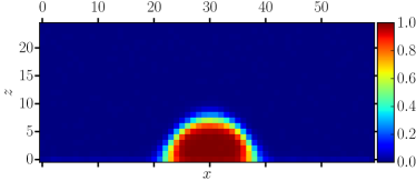
Figure 1: Density profile of the pseudo 2D droplet used to create the ridge in the MC system for the parameter set P2.

This particle density profile is used to generate the initial ridge of length $L_{y}$ oriented in the $y$-direction. For every value of the coordinate $y=0,..,L_{y}-1$, an individual configuration is generated by randomly assigning a particle number on $x$ and $z$ positions following the probabilities as given by the density profile. By this procedure, a well defined realization of a ridge on the lattice is formed. The pre-structure is represented by more attractive sites $g_{\bf i}$, which are incorporated into the substrate plane where they replace the substrate sites $s_{\bf i}$ in a region of width $w$ at the center of the domain. This pattern is then continued in the $y$-direction thereby forming a more wettable stripe of width $w$. The initial ridge is created centered on this stripe in the same way as described above. Note that for both parameter sets, the fluid is partially wetting, in particular, the pre-patterned stripe has a smaller contact angle than the bare substrate. All simulations are then repeated multiple times to obtain a statistical description.

III Transversal Instabilities

III.1 Single Ridge on Pre-patterned Substrate

As a model system which is of great relevance for experiments, we study the instability of a single ridge formed on top of a pre-pattern stripe. On homogeneous substrates, such ridge solutions are always unstable with respect to transversal modulations (see Mechkov et al. (2007); Thiele et al. (2003)). As shown, e.g., in Honisch et al. (2015), the pre-pattern can stabilize the structure for certain regions of parameter space spanned by the pre-pattern strength, pre-pattern size and the liquid volume in the ridge. Here, we focus on the regime where the ridge is transversally unstable. However, the broken translational invariance of the substrate in $x$-direction simplifies the investigations of the large scale behavior through the KMC simulations, since translational fluctuations of the ridge are reduced.

In Fig. 2 (b),(d), the transversal instabilities and the resulting bulges on top of the pre-pattern are shown for the two different models. In addition, as a measure for the volume of molecules that are redistributed along the ridge, in Fig. 2 (a),(c), we show for each model the time-evolution of the amplitudes of the first harmonic modes of the field integrated in $x$- and $z$-direction. For the discrete KMC model, these quantities are determined as the absolute values of the discrete Fourier transform of the occupation field summed over $x$ and $z$ at a given transversal wavenumber $k_{y}$. It reads:

$$\left|\mathcal{FT}[m_{y}](k_{y},t)\right|= \left|\sum_{n_{y}=0}^{L_{y}-1}m_{y}(n_{y},t)e^{-2\pi i\frac{n_{y}k_{y}}{L_{y}}}\right|,$$ (7)

$$m_{y}(n_{y},t)= \sum_{n_{x},n_{z}}P(n_{x},n_{y},n_{z}),$$ (8)

where $P(n_{x},n_{y},n_{z})$ is the occupation field of the ridge. For the continuum model, the analogue of these quantities is defined through the continuous Fourier transform of the height profile integrated over $x$:

$$\left|\mathcal{FT}[m_{y}](k_{y},t)\right| =\left|\int m_{y}(y,t)e^{-2\pi i\frac{k_{y}y}{L_{y}}}\mathrm{d}y\right|,$$ (9)

$$m_{y}(y,t) =\int h(x,y,t)\mathrm{d}x.$$ (10)

The absolute values of the Fourier transform are shown individually for the first harmonic modes of re-distribution, in particular, for wavenumbers $k_{y}=1,2,3$.

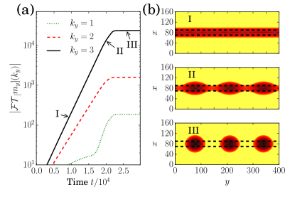
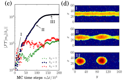
Figure 2: (a) Plot of the absolute value of the Fourier transform $\left|\mathcal{FT}[m_{y}]\right|$ (modes $k_{y}=1,2,3$) over time in logarithmic presentation for the evolution of the transversal instability of a single ridge in a DNS of the thin-film model Eq. (1). Corresponding snapshots are given in (b). The mean film height is $h_{0}=2.25$, further system parameters are $\rho=0.2$, $l_{s}=3.0$ and the stripe width $w=20$. The dashed lines in (b) visualize the borders of the more wettable region. (c) Analogue plot of the absolute value of the Fourier transform (modes $k_{y}=1,2,3$) over time $n\Delta t$ for the evolution of the transversal instability of a single ridge obtained in a KMC simulation for parameter set P2, a system size of $L_{y}=160a$ and $w=10a$. (d) Corresponding snapshots.

For the continuum model, the instability develops through a rather extended phase of exponential growth that corresponds to the linear instability regime. As expected due to the non-deterministic nature of the model, in the KMC simulations this regime is influenced by noise. However, an exponential growth regime of the $k_{y}=2$ mode can be clearly identified. After the initial regime of linear instability, both models show a nonlinear phase in which the ridge decays into separated droplets via pinch-off events. Although the system is clearly in the nonlinear regime in the later stages of the pinch-off process, the growth of $\left|\mathcal{FT}[m_{y}]\right|$ remains surprisingly exponential in the early stage of this process, still approximately with the same growth rate as in the initial regime. A surprisingly long-lasting linear behavior has been reported before for the Cahn-Hilliard equation Sander and Wanner (2000). The transversal instability and its dependency on system parameters will now be analyzed in more detail for both models.

III.1.1 Analysis of the Instability for the Continuum Model

In the case of the continuum model, the dispersion relation and the shape of the unstable modes can be obtained in a standard linear stability analysis that results in an eigenvalue problem which is solved numerically.

Denoting a one-dimensional steady state (stable or unstable) by $h_{0}(x)$, a linear stability analysis w.r.t. transversal instability modes is performed employing the ansatz

$$h(x,y,t)=h_{0}(x)+h_{1}(x)e^{\beta t+2\pi i\frac{k_{y}y}{L_{y}}}.$$ (11)

Note that $k_{y}$ in the exponential ansatz is scaled by $2\pi/L_{y}$, so that its definition coincides with the one used in Eq. (9). Then, $2\pi k_{y}/L_{y}$ corresponds to the typically employed system size-independent wavenumber. As described in more detail in Honisch et al. (2015); Thiele et al. (2003), this ansatz combined with a linearization of Eq. (1) leads to the eigenvalue problem

$$\mathcal{L}[h_{0}(x),k_{y}]h_{1}(x)=\beta h_{1}(x),$$ (12)

where the eigenvalue $\beta$ of the linear operator $\mathcal{L}[h_{0}(x),k_{y}]$ corresponds to the growth rate of transversal modulations with the wavenumber $k_{y}$. The linear operator depends on the mobility function ($M(h)$ in Eq. (1)). Although the stability criterion can be obtained by purely energetic considerations based on capilarity and wettability, the specific form of the dynamical equation influences the dispersion relation. In particular, to obtain the fastest growing unstable mode, the full dynamical equation has to be considered. Droplets formed in accordance with the resulting wavelength might exist for a long transient before successive coarsening Honisch et al. (2015). In realistic experiments, the final post-coarsening equilibrium state of a single drop is often not reached, i.e. the dynamical pathway is of interest.

In Fig. 3 (a), we show the one-dimensional steady state solution $h_{0}$ as well as the eigenfunction $h_{1}$ for the fastest growing wavenumber. The parameters correspond to the ones of the direct numerical simulations (DNS) in Fig. 2 (a),(b).

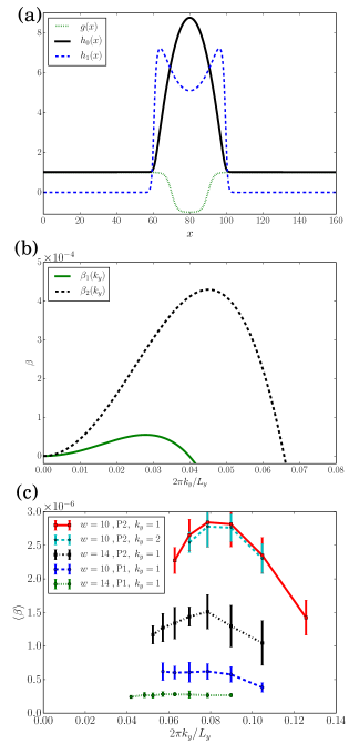
Figure 3: (a) For the thin-film model, we show a one-dimensional steady state $h_{0}(x)$ (ridge cross-section), pre-pattern function $g(x)$ and unstable transversal mode $h_{1}(x)$ at $k_{y,\mathrm{max}}$. The parameters are $h_{0}=2.25$, $\rho=0.2$, $w=20$. (b) Dispersion relations of the transversal instability of a single ridge for two different pre-pattern stripe widths. For $\beta_{1}$ and $\beta_{2}$, we chose $w=40$ and $w=20$, respectively. All other parameters are as above. (c) Dispersion relations extracted from the MC simulations, P1 and P2 refer to the parameter sets given in section II.2. The growth rate is determined by fitting the exponential regime of $\left|\mathcal{FT}[m_{y}]\right|$ for the selected mode. The errorbars represent the standard deviation of the averaging procedure.

By numerical continuation techniques, the unstable eigenvalue and the corresponding eigenfunction are followed in $k_{y}$ to obtain the transversal dispersion relation (see Fig. 3(b)). The dispersion relation is reminiscent of a fourth order polynomial but can only be described approximately by such a function due to the dependence of the eigenfunction on $k_{y}$ that results in contributions that are higher order in $k_{y}$. At $k_{y}=0$, the eigenfunction $h_{1}$ has a bimodal form and corresponds to the neutral growth mode. The growth rate is zero for $k_{y}=0$, as imposed by the mass conserving dynamics of the form $\partial_{t}h=-\nabla\cdot\mathbf{J}$ of Eq. (1) and the non-vanishing integral of the eigenfunction $h_{1}$. We show the dispersion relation for the stripe width employed in the DNS and for another, larger stripe width where eventually, for larger values of $\rho$ than the one shown in Fig. 3 (b), pinning of the contact line and stabilization of the ridge occurs.

III.1.2 Analysis of the Instability for the KMC Model

For the KMC model, the dispersion relations for the transversal instability can only be determined by direct numerical simulations. Furthermore, as already discussed at Fig. 2(c),(d), the initial, linear regime of the instability in the KMC simulations is influenced by noise, such that the linear growth rate is neither always present nor unique if individual simulations are considered. Nonetheless, one may determine the growth rate in a statistical sense. To do so, we consider systems of different longitudinal size $L_{y}$ and determine $\left|\mathcal{FT}[m_{y}]\right|$ for the dominant mode, compare Fig. 2 (c). In analogy to the dispersion relation obtained with the continuum model, for small values of $L_{y}$, the modes with $k_{y}=1$ dominate. Increasing $L_{y}$, eventually higher modes become dominant what implies that only a $k_{y}$-range around the maximum of the dispersion relation can be obtained. The results are shown in Fig. 3 (c). For $w=10$ and P2, the results for the growth rate of the $k_{y}=1$ modes are confirmed by a corresponding analysis for the second mode ($k_{y}=2$) using a system twice as large. For each system size at least 10 appropriate $\left|\mathcal{FT}[m_{y}]\right|$ curves are recorded and fitted by a function of the form $f(t)=ae^{\beta t}$ for an appropriate time range. Only fits with a maximum fit-error of 3% are considered and averaged in order to obtain the mean growth rate $\langle\beta\rangle$. The results of this procedure are shown in Fig. 3 (c) for the two parameter sets and pre-pattern stripe widths $w=10$ and $w=14$. As expected, only growth rates around the maximum of the dispersion relation can be extracted. For larger $L_{y}$, the instability is naturally dominated by higher modes close to the maximum of the dispersion relation, i.e., small $k_{y}$ values can not be accessed by looking at the dominant modes. For smaller $L_{y}$ (larger $k_{y}$) there is a sharp decrease towards zero, which could not be better resolved with the present statistics (compare to continuum model Fig. 3 (b)). Overall, we find that the dispersion relations extracted from the KMC simulations qualitatively well agree with the ones determined with the continuum model. Note, however, that due to the fluctuations in the system, lower growth rates are more difficult to extract.

At higher temperatures (i.e., case P2), the maxima of the dispersion relations are higher and can therefore be extracted more precisely, even though the larger fluctuations imply larger variances. In continuum models, an increased temperature can be reflected in increased transport coefficients. In the particular thin-film model Eq. (1) used, this would correspond to a decreased value of the viscosity $\eta$. Assuming that this effect dominates an also possible effect on the wetting behavior (decreasing contact angle with increasing temperature), one finds that the growth rate of the instability which is inversely proportional to the viscosity, increases with temperature. This is consistent with the corresponding effect seen in the KMC simulations (Fig. 3 (c)).

III.2 Two Weakly Interacting Ridges on Pre-patterned Substrate

The second pre-pattern geometry we consider is a system with two neighboring more-wettable stripes. The distance $d$ between the stripes does not correspond to the periodicity of the simulation domain imposed by the boundary conditions. The question addressed by this investigation is how the weak interaction of two liquid ridges on the two stripes influences their instability. For the continuum model, we perform a similar linear stability analysis as for the one-stripe system above. For a symmetric two-ridge solution (one ridge on each stripe, both identical), we find two different transversal instability modes as shown in Fig. 4 (a).

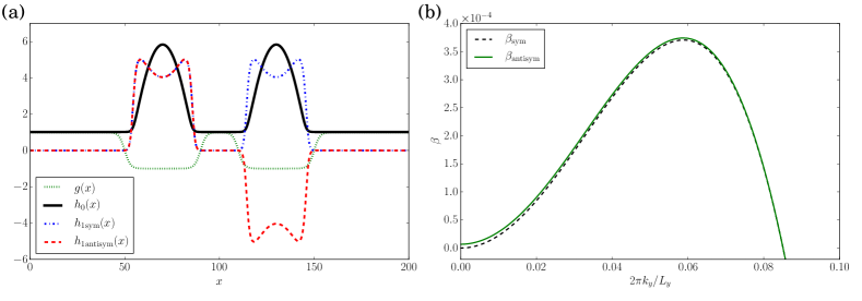
Figure 4: (a) For the thin-film model of the two-stripe system, we show a one-dimensional steady state $h_{0}(x)$ (cross-section of ridges), the pre-pattern function $g(x)$ and the symmetrical and antisymmetrical unstable transversal modes $h_{1,\mathrm{sym}}(x)$ and $h_{1,\mathrm{antisym}}(x)$, respectively, both at $k_{y,\mathrm{max}}$. Parameters are $h_{0}=2.0$, $\rho=0.2$, $w=40$, $l_{s}=3$, $d=20$ (distance of the stripes).
(b) Corresponding dispersion relations of the two unstable transversal instability modes. The dispersion relation of the symmetric mode approaches zero at $k_{y}=0$ due to mass conservation while the one of the antisymmetric mode approaches at $k_{y}=0$ a non-zero growth rate corresponding to the coarsening mode due to mass transfer of 1d drops, demonstrating the interaction of the ridges.

The first mode, denoted by $h_{1,\mathrm{sym}}$, can be seen in analogy to the instability mode for the one-stripe system and proceeds through periodic transversal mass transfer (i.e., along each ridge) equally and synchronously in both ridges. The eigenvalue of this mode goes to zero at $k_{y}=0$ as dictated by mass conservation, compare Fig. 4 (b).

The second, antisymmetric mode $h_{1,\mathrm{antisym}}$ shown in Fig. 4 (a), corresponds to mass transfer along each ridge and between the two ridges in such a way that the drop patterns developing on the two ridges are shifted w.r.t. each other by half a period. This is a signature of the weak interaction of the two ridges. Note that the growth rate of the antisymmetric mode approaches a finite non-zero value at $k_{y}=0$. In this case, the mode corresponds to the coarsening mode due to mass transfer known for 1d drops Thiele et al. (2003); Thiele (2007).

For the dominant values of $k_{y}$, the growth rates of the two unstable modes are almost identical, the one of the antisymmetric mode is only slightly larger. Therefore, the mode dynamically chosen by the system is arbitrary - it may be either of the two or some linear combination. In the specific simulation of the continuum model, shown in Fig. 5 (a), the system exhibits an instability dominated by the antisymmetric mode, thus forming a configuration of alternating drops, which are subjected to slow coarsening.

In the corresponding simulation with the KMC model shown in Fig. 5 (b), one also observes a break up of the two ridges in an alternating manner, thus also there the antisymmetric instability mode dominates.

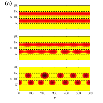
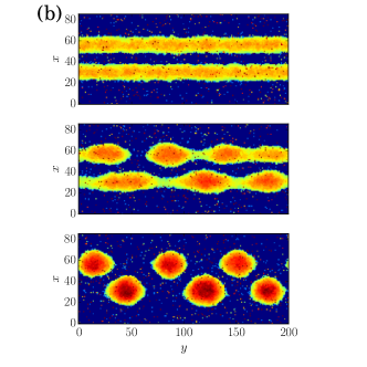
Figure 5: Snapshots from numerical simulations of the transversal instability of two weakly interacting ridges on pre-pattern stripes. (a) shows results for the thin-film model at parameters $h_{0}=2.0$, $\rho=0.2$, $w=40$, $d=20$. In (b), we give the corresponding results for the KMC simulations at parameters $w=10a$, $d=16a$, $L_{y}=200a$ and set P2 of interaction constants.

IV Conclusion and outlook

We have investigated the Plateau-Rayleigh instability of ridges of molecules on pre-patterned substrates by means of two inherently different modeling approaches, namely, a stochastic discrete kinetic Monte Carlo (KMC) model and a deterministic continuum hydrodynamic thin-film model.

We have systematically shown that despite the different nature of the approaches, the results are in very good qualitative agreement. In particular, the dynamics of the transversal ridge instabilities seen with the KMC model on large time and length scales (compared to the microscopic one of individual hopping events) is consistent with the transversal instabilities as analyzed in the thin-film model: A comparison of the Fourier analyses of typical time evolutions of single ridges has shown that in both models one can identify long regimes of exponential growth followed by droplet pinch-off. The extended exponential regime has allowed us to extract dispersion relations from the KMC model via a fitting and averaging procedure. A comparison with dispersion relations obtained via standard linear stability analysis within the thin-film model, i.e., by the solution of the corresponding linear eigenvalue problem, has shown a good qualitative agreement of the two approaches. Likewise, we have demonstrated a qualitative agreement of the evolution pathway in the two-stripe system where in both models an antisymmetric droplet pattern can evolve from the transversal instability. Therefore, also there the linear stability result from the thin-film model could be reproduced in the KMC simulations.

The focus of the present work has been on the qualitative agreement of a stochastic discrete and a deterministic continuum modeling approach in the context of a specific, experimentally relevant system. However, we would like to add a few remarks on the nature of the agreement between the approaches and outline how a quantitative mapping may be reached between averaged KMC simulations and a mesoscopic gradient dynamics (or thin-film) model for the evolution of the film height profile.

As already emphasized in the introduction, to reach a quantitative correspondence between the two models is a non-trivial task, since the underlying physical assumptions about the system are not identical. While the KMC model assumes a diffusive dynamics with exclusively short-ranged particle interactions, the thin-film model is derived from the standard equation for overdamped hydrodynamics, namely the Stokes equation.

A first step in order to achieve a quantitative mapping between the models would be to map the models in terms of their equilibrium behavior, i.e., their statics/energetics. Here, one may consider a mean field approximation of the KMC model in terms of a classical lattice density functional theory (DFT) approximation. This could be done for the case of different homogeneous substrates to then apply the results to the heterogeneous case. In Hughes et al. (2015), it is shown how one is able to extract the interface tension and the effective wetting potential from appropriate lattice DFT theories with different interaction ranges (cf. MacDowell and Müller (2005); Tretyakov et al. (2013) for an alternative approach via a Molecular Dynamics MD simulations). The resulting interface Hamiltonian (or free energy) is then incorporated into a mesoscopic continuum theory in gradient dynamics form and it is shown that height profiles of mean field droplets obtained from the lattice DFT are accurately reproduced. As explained above, the effective wetting potential directly gives the Derjaguin (or disjoining) pressure that appears in the thin-film equation.

Such a mapping on a purely energetic level does not only allow one to investigate static ridge and droplet states but also to assess their stability either via a second variation of the free energy or via a dynamical approach. For the latter, one assumes that the dynamics follows a gradient dynamics on the interface Hamiltonian. For instance, for a thin-film equation like Eq. (1), Mechkov et al. (2007) shows that the threshold of the transversal instability is entirely encoded in the energy functional. To fully account for the dynamics one needs to take a further step and extract from stochastic discrete models as the KMC model the full mobility functions that enter the thermodynamic fluxes in the gradient dynamics form of the thin-film type model Eq. (1). This could be done by a direct numerical fitting process or analytically, starting from a Cahn-Hilliard type dynamical mean field model such as the one discussed in Monson (2008). However, the employed stochastic model(s) should allow for the extraction of all effective transport parameters, i.e., diffusion constant, slip length and viscosity to fully account for transport by diffusion at very small (sub-monolayer) film height and by advection at larger film height. A discussion of these transport modes in the context of a thin-film evolution equation with a general polynomial mobility function may be found in Yin et al. (2017).

References

- Yoon et al. (2008) B. Yoon, H. Acharya, G. Lee, H.-C. Kim, J. Huh, and C. Park, Soft Matter 4, 1467 (2008).
- Seemann et al. (2005) R. Seemann, M. Brinkmann, E. J. Kramer, F. F. Lange, and R. Lipowsky, Proc. Natl. Acad. Sci. U. S. A. 102, 1848 (2005).
- Kargupta and Sharma (2001) K. Kargupta and A. Sharma, Phys. Rev. Lett. 86, 4536 (2001).
- Sehgal et al. (2002) A. Sehgal, V. Ferreiro, J. F. Douglas, E. J. Amis, and A. Karim, Langmuir 18, 7041 (2002).
- Zhang et al. (2003) Z. Zhang, Z. Wang, R. Xing, and Y. Han, Polymer 44, 3737 (2003).
- Mukherjee et al. (2008) R. Mukherjee, D. Bandyopadhyay, and A. Sharma, Soft Matter 4, 2086 (2008).
- Konnur et al. (2000) R. Konnur, K. Kargupta, and A. Sharma, Phys. Rev. Lett. 84, 931 (2000).
- Gau et al. (1999) H. Gau, S. Herminghaus, P. Lenz, and R. Lipowsky, Science 283, 46 (1999).
- Lied et al. (2012) F. Lied, T. Mues, W. Wang, L. Chi, and A. Heuer, J. Chem. Phys. 136, 024704 (2012).
- Brinkmann and Lipowsky (2002) M. Brinkmann and R. Lipowsky, J. Appl. Phys. 92, 4296 (2002).
- Bauer and Dietrich (2000) C. Bauer and S. Dietrich, Phys. Rev. E 61, 1664 (2000).
- Lenz and Lipowsky (1998) P. Lenz and R. Lipowsky, Phys. Rev. Lett. 80, 1920 (1998).
- Kargupta et al. (2000) K. Kargupta, R. Konnur, and A. Sharma, Langmuir 16, 10243 (2000).
- Thiele et al. (2003) U. Thiele, L. Brusch, M. Bestehorn, and M. Bär, Eur Phys J E Soft Matter 11, 255 (2003).
- Mechkov et al. (2008) S. Mechkov, M. Rauscher, and S. Dietrich, Physical Review E 77, 061605 (2008).
- Koplik et al. (2006) J. Koplik, T. Lo, M. Rauscher, and S. Dietrich, Phys. Fluids 18, 032104 (2006).
- Wang et al. (2011) W. Wang, C. Du, C. Wang, M. Hirtz, L. Li, J. Hao, Q. Wu, R. Lu, N. Lu, Y. Wang, et al., small 7, 1403 (2011).
- Wang and Chi (2012) W. Wang and L. Chi, Acc. Chem. Res. 45, 1646 (2012).
- Wang et al. (2016) H. Wang, O. Buller, W. Wang, A. Heuer, D. Zhang, H. Fuchs, and L. Chi, New J. Phys. 18, 053006 (2016).
- Honisch et al. (2015) C. Honisch, T.-S. Lin, A. Heuer, U. Thiele, and S. V. Gurevich, Langmuir 31, 10618 (2015).
- King et al. (2006) J. R. King, A. Münch, and B. Wagner, Nonlinearity 19, 2813 (2006).
- Beltrame et al. (2011) P. Beltrame, E. Knobloch, P. Hänggi, and U. Thiele, Phys. Rev. E 83, 016305 (2011).
- Eggers (1997) J. Eggers, Rev. Mod. Phys. 69, 865 (1997).
- Plateau (1873) J. A. F. Plateau, Statique Expérimentale et Théorique des Liquides Soumis aux Seules Forces Moléculaires (Gauthier-Villars, Paris, 1873).
- Savart (1833) F. Savart, Annal. Chim. 53, 337 (1833), plates in Vol. 54.
- Rayleigh (1878) L. Rayleigh, Proceedings of the London mathematical society 10, 4 (1878).
- Müller et al. (2002) T. Müller, K.-H. Heinig, and B. Schmidt, Mater Sci Eng C Mater Biol Appl 19, 209 (2002).
- Oron et al. (1997) A. Oron, S. H. Davis, and S. G. Bankoff, Rev Mod Phys 69, 931 (1997).
- Mitlin (1993) V. S. Mitlin, J. Colloid Interface Sci. 156, 491 (1993).
- Thiele (2010) U. Thiele, J. Phys.: Condens. Matter 22, 084019 (2010).
- Pismen (2001) L. Pismen, Physical Review E 64, 021603 (2001).
- Savva and Kalliadasis (2011) N. Savva and S. Kalliadasis, Europhys. Lett. 94, 64004 (2011).
- Schick (1990) M. Schick, in Liquids at Interfaces, Proceedings of the Les Houches Summer School in Theoretical Physics, Session XLVIII (North-Holland, Amsterdam, 1990).
- Hughes et al. (2015) A. P. Hughes, U. Thiele, and A. J. Archer, J Chem Phys 142, 074702 (2015).
- Dietrich (1988) S. Dietrich, in Phase Transitions and Critical Phenomena, Vol. 12, edited by C. Domb and J. L. Lebowitz (Academic Press, London, 1988) p. 1.
- Pismen and Thiele (2006) L. M. Pismen and U. Thiele, Phys Fluids (1994) 18, 042104 (2006).
- Glasner and Witelski (2003) K. B. Glasner and T. P. Witelski, Physical review E 67, 016302 (2003).
- Bastian et al. (2008a) P. Bastian, M. Blatt, A. Dedner, C. Engwer, R. Klöfkorn, M. Ohlberger, and O. Sander, Computing 82, 103 (2008a).
- Bastian et al. (2008b) P. Bastian, M. Blatt, A. Dedner, C. Engwer, R. Klöfkorn, R. Kornhuber, M. Ohlberger, and O. Sander, Computing 82, 121 (2008b).
- Bastian et al. (2010) P. Bastian, F. Heimann, and S. Marnach, Kybernetika 46, 294 (2010).
- Alexander (1977) R. Alexander, SIAM J Numer Anal 14, 1006 (1977).
- Kawasaki (1972) K. Kawasaki, “Phase transitions and critical phenomena,” (Academic Press, 1972) p. 443.
- Metropolis et al. (1953) N. Metropolis, A. W. Rosenbluth, M. N. Rosenbluth, A. H. Teller, and E. Teller, J. Chem. Phys. 21, 1087 (1953).
- Mechkov et al. (2007) S. Mechkov, G. Oshanin, M. Rauscher, M. Brinkmann, A. Cazabat, and S. Dietrich, Europhys. Lett. 80, 66002 (2007).
- Sander and Wanner (2000) E. Sander and T. Wanner, SIAM J Appl Math 60, 2182 (2000).
- Thiele (2007) U. Thiele, in Thin Films of Soft Matter, edited by S. Kalliadasis and U. Thiele (Springer, Wien, 2007) pp. 25–93.
- MacDowell and Müller (2005) L. MacDowell and M. Müller, J. Phys.-Condes. Matter 17, S3523 (2005).
- Tretyakov et al. (2013) N. Tretyakov, M. Müller, D. Todorova, and U. Thiele, J. Chem. Phys. 138, 064905 (2013).
- Monson (2008) P. A. Monson, J Chem Phys 128, 084701 (2008).
- Yin et al. (2017) H. Yin, D. Sibley, U. Thiele, and A. Archer, Phys. Rev. E 95, 023104 (2017).