-based star formation laws in hierarchical models of galaxy formation
Abstract
We update our recently published model for GAlaxy Evolution and Assembly (GAEA), to include a self-consistent treatment of the partition of cold gas in atomic and molecular hydrogen. Our model provides significant improvements with respect to previous ones used for similar studies. In particular, GAEA (i) includes a sophisticated chemical enrichment scheme accounting for non-instantaneous recycling of gas, metals, and energy; (ii) reproduces the measured evolution of the galaxy stellar mass function; (iii) reasonably reproduces the observed correlation between galaxy stellar mass and gas metallicity at different redshifts. These are important prerequisites for models considering a metallicity dependent efficiency of molecular gas formation. We also update our model for disk sizes and show that model predictions are in nice agreement with observational estimates for the gas, stellar and star forming disks at different cosmic epochs. We analyse the influence of different star formation laws including empirical relations based on the hydrostatic pressure of the disk, analytic models, and prescriptions derived from detailed hydrodynamical simulations. We find that modifying the star formation law does not affect significantly the global properties of model galaxies, neither their distributions. The only quantity showing significant deviations in different models is the cosmic molecular-to-atomic hydrogen ratio, particularly at high redshift. Unfortunately, however, this quantity also depends strongly on the modelling adopted for additional physical processes. Useful constraints on the physical processes regulating star formation can be obtained focusing on low mass galaxies and/or at higher redshift. In this case, self-regulation has not yet washed out differences imprinted at early time.
keywords:
galaxies: formation – galaxies: evolution – galaxies: star formation – galaxies: ISM1 Introduction
A proper description of how galaxies form and evolve requires necessarily an understanding of the physical mechanisms regulating the star formation process within dense regions of molecular clouds. At the microscopic level, star formation arises from a complex interplay between e.g. turbulence, rotation and geometry of the cloud, and magnetic fields, making a self-consistent treatment of the process from ‘first principles’ unfeasible in theoretical models of galaxy formation and evolution. Fortunately, clear and tight correlations are measured between the rate at which stars form within a (disc) galaxy and the amount of gas in the disc. Such correlations have, for decades now, been a crucial element of theoretical models of galaxy formation.
One commonly adopted star formation formulation is based on the so-called Schmidt-Kennicutt law (Schmidt, 1959; Kennicutt, 1998), which relates the surface density of the star formation rate to that of the gas via a simple power law: , with 111Kennicutt (1998) show that a formulation that assumes the surface density of star formation rate scales with the ratio of the gas density to the average orbital time scale, fitted their data equally well.. In many galaxy formation models, a slightly different formulation is used, which assumes the star formation rate declines rapidly for surface densities below a critical value, often estimated using the disk stability criterion introduced by Toomre (1964). For the sample presented in Kennicutt (1998), the correlation between and (including both molecular and atomic hydrogen) was stronger than that with the surface density of molecular gas . Albeit this and earlier work pointed out that the larger scatter of the latter relation could be at least in part due to variations in the CO/H2 conversion factor, most models up to a few years ago simply assumed that the star formation rate depends on the amount (and/or surface density) of ‘cold gas’ (typically all gas below K), with no attempt to partition it in its molecular and atomic components.
In the last decade, our phenomenological understanding of star formation in galaxies has improved significantly thanks to the advent of high-quality spatially resolved observations in HI (e.g. the HI Nearby Galaxy Survey - Walter et al., 2008) and CO, (e.g. The BIMA Survey of Nearby Galaxies - Helfer et al. 2003, and The HERA CO Line Extragalactic Survey - Leroy et al. 2009) and, at the same time, of more reliable estimates of the star formation at different wavelengths for large samples of nearby galaxies (e.g. The Spitzer Infrared Nearby Galaxies Survey - Kennicutt et al. 2007; Calzetti et al. 2007, and the Galaxy Evolution Explorer Nearby Galaxies Survey - Gil de Paz et al. 2007). These data clearly demonstrate that star formation correlates strongly with the molecular gas in a galaxy, and poorly or not at all with the atomic gas (e.g. Wong & Blitz, 2002; Kennicutt et al., 2007; Leroy et al., 2008). In non-barred spiral galaxies, the fraction of molecular gas increases towards the centre, where the HI gas surface density remains flat or weakly declines (Bigiel et al., 2008). The threshold in star formation suggested by early observations (Kennicutt, 1989; Martin & Kennicutt, 2001) can therefore be interpreted as a transition to a different regime of star formation activity. Although it is unclear if molecular gas is a necessary condition for star formation (see e.g. Glover & Clark, 2012; Hu et al., 2016, and references therein), The observational data provide a detailed characterization of the star formation law in terms of molecular hydrogen.
Based on a relatively small sample of nearby galaxies, Blitz & Rosolowsky (2006) argue that the ratio of molecular-to-atomic hydrogen surface density is determined by the hydrostatic pressure of the disk. The scatter in the Blitz & Rosolowsky (2006) relation is relatively large, and alternative interpretations have been provided for the observations. A different view considers the molecular fraction as determined by a balance between the production of molecular hydrogen on the surface of dust grains and dissociation of the molecules by radiation from young stars (Krumholz, McKee & Tumlinson, 2009b; Gnedin & Kravtsov, 2011).
While the physical processes regulating star formation remain to be understood, the new rich phenomenology described above has also triggered significant activity devoted to update and test the influence of H2 based star formation laws both in hydrodynamical simulations (e.g. Gnedin & Kravtsov, 2011; Kuhlen et al., 2012), and in semi-analytic models of galaxy formation (e.g. Fu et al., 2010; Lagos et al., 2011b; Somerville, Popping & Trager, 2015). Given their flexibility and limited computational costs, the latter represents an ideal interpretative tool for large ongoing surveys of cold gas in nearby and distant galaxies (Fu et al., 2012; Lagos et al., 2011a; Popping, Somerville & Trager, 2014), as well as future projects planned on facilities such as the Atacama Large Millimeter/sub-millimeter Array (ALMA - Wootten & Thompson, 2009), the Square Kilometre Array (SKA - Carilli & Rawlings, 2004) and its pathfinders (Booth et al., 2009; Johnston et al., 2008), and the Five-hundred-meter Aperture Spherical radio Telescope (FAST - Nan et al., 2011).
In this work, we extend our new and recently published semi-analytic model for GAlaxy Evolution and Assembly (GAEA) by including an explicit treatment for the partition of cold gas in its atomic and molecular component. As one of its major features, GAEA includes a sophisticated scheme for chemical enrichment based on non-instantaneous recycling of gas, energy and metals (De Lucia et al., 2014). Hirschmann, De Lucia & Fontanot (2016) show that GAEA also successfully reproduces the evolution of the observed correlation between the galaxy stellar mass and cold gas metallicity - an important prerequisite for schemes that assume the molecular-to-atomic ratio depends on the gas metallicity.
This paper is organized as follows: in Section 2, we introduce our semi-analytic model and describe in detail the star formation laws that we considered. In Section 3, we describe how these different star formation laws affect the physical properties of galaxies, and compare basic statistics on the distribution of stellar masses, HI and H2 with available data. In Section 4, we compare model predictions with observed scaling relations between the amount of molecular and atomic hydrogen, gas metallicity, size of the star forming discs and galaxy stellar mass. In Section 6, we discuss our results also in the framework of previous work. Finally, in Section 7, we summarize our findings and give our conclusions.
2 Semi-analytic model
In this work, we take advantage of our recently published model GAEA (Hirschmann, De Lucia & Fontanot, 2016, hereafter HDLF16). This model builds on that described in De Lucia & Blaizot (2007), with modifications introduced to follow more accurately processes on the scales of the Milky Way satellites (De Lucia & Helmi, 2008; Li, De Lucia, & Helmi, 2010). The evolution of the baryonic component of dark matter haloes is traced by following four different reservoirs: stars in galaxies, cold gas in the galaxy discs, diffuse hot gas associated with dark matter haloes, and an ejected gas component. The transfer of mass and energy between these components is modelled assuming specific prescriptions for: gas cooling, star formation, stellar feedback (including metal enrichment, reheating of cold gas, and gas ejection), galaxy mergers (and associated star-bursts), bulge formation during mergers and driven by disk instability. The model also includes prescriptions for cold (merger driven) and hot gas accretion onto super massive black holes, and for the suppression of cooling flows in massive haloes from radio loud Active Galactic Nuclei (AGN).
Our physical model for the evolution of the baryonic components of galaxies is coupled to the output of cosmological dark matter simulations, as detailed in De Lucia & Blaizot (2007). In this study, we use dark matter merger trees from two large-scale cosmological simulations: the Millennium Simulation (Springel et al., 2005, MS), and the Millennium II Simulation (Boylan-Kolchin et al., 2009, MSII). Both simulations consist of particles; the box size is for the MS and for the MSII, while the particle mass is for the MS and for MSII. Both simulations assume a WMAP1 cosmology, with , , , , and . Recent measurements from PLANCK (Planck Collaboration et al., 2015) and WMAP9 (Bennett et al., 2013) provide slightly different cosmological parameters and, in particular, a larger value for and a lower one for . As shown in previous work, however, these differences are expected to have little influence on model predictions, once model parameters are returned to reproduce a given set of observables in the local Universe (Wang et al., 2008; Guo et al., 2013).
In the following, we will briefly summarize the physical prescriptions that are relevant for this work, and discuss in detail our modifications to include a modelling of star formation that depends on the amount of molecular hydrogen.
2.1 Star formation and stellar feedback in the GAEA model
In our work, we will assume as a reference ‘fiducial’ model the one presented in HDLF16 including prescriptions for stellar feedback based on the FIRE simulations, plus the modifications discussed below in Sections 2.2 and 2.3.
In this model, the rate of star formation depends on the amount of ‘cold gas’, defined as all gas with temperature below K, associated with a model galaxy. In particular, we assume:
| (1) |
where is the efficiency at which gas is converted into stars, and is the dynamical time of the galaxy. is the radius of the star forming region. We assume this is equal to times the scale length of the disk (assuming an exponential profile, as in our case, this means that the star forming region includes per cent of the total gas mass). is the virial velocity of the parent substructure (or the virial velocity at the last time there was a resolved subhalo for orphan galaxies.)
is the amount of gas available for star formation. Following De Lucia & Helmi (2008), this is computed by integrating the surface density of the cold gas disk, assumed to be exponential, out to the radius () at which the gas surface density drops below the following critical value (Kennicutt, 1989):
| (2) |
GAEA features a detailed treatment for chemical enrichment that accounts for the finite lifetime of stars and its dependence on stellar mass, and allows us to trace individual chemical abundances and non-instantaneous recycling of metals, gas, and energy. We refer to De Lucia et al. (2014) for a detailed description of the relevant prescriptions. Briefly, our model includes separate sets of chemical yields for Asymptotic Giant Branch stars (AGBs) and both Supernovae Type Ia (SnIa - the main contributors of iron-peak elements) and Type II (SnII - that mainly release elements, including O, Mg, Si, S, Ca). The assumed delay time distribution for SnIa corresponds to a fraction of prompt222‘Prompt’ is here defined as exploding within yr from the star formation episode. The fraction increases to about 23 per cent when considering SnIa events within yr. SnIa of about 5 per cent. When a star formation event takes place, our code stores the information about the metals, energy and mass of Helium and Hydrogen that will be available at any time in the future. These information are then included as galaxy evolution proceeds forward in cosmic time. De Lucia et al. (2014) argue that this approach provides a more accurate accounting of the timings and properties of individual star formation events than alternative methods based on the storage and binning of the past star formation history of model galaxies. We note that all previous semi-analytic models that include an explicit treatment of the partition between atomic and molecular gas (Fu et al., 2010; Lagos et al., 2011b; Somerville, Popping & Trager, 2015) are based on an instantaneous recycling approximation.
The energy released by supernovae and stellar winds is assumed to reheat some of the cold gas in the disk and to drive large-scale galactic winds, ejecting gas out of the parent halo. Our model for stellar feedback is based on parametrizations extracted from the FIRE hydrodynamical simulations (Hopkins et al., 2014; Muratov et al., 2015). Specifically, the reheating rate of the cold gas depends on the star formation rate and scales both with redshift and with the potential well of the galaxy:
| (3) |
is the maximum circular velocity of the parent halo. When , the index is , while for larger values of , . The reheating efficiency, is assumed to be constant and equal to . The total energy released by massive stars can be expressed as:
| (4) |
where is the mean kinetic energy of SN ejecta per unit mass of stars formed, and is the ejection efficiency. An ejection rate can then be computed as:
| (5) |
Following the approach by Henriques et al. (2013), we assume that ejected gas can be re-accreted on a time-scale that depends on the virial mass of the parent halo.
As discussed in HDLF16, this stellar feedback scheme allows us to to reproduce the measured evolution of the galaxy stellar mass function, and the observed correlation between galaxy stellar mass and its gaseous/stellar metallicity content. In particular, this model also reproduces the observed evolution of the mass-cold gas metallicity relation to higher redshift. This is an important aspect of our reference model since some of the star formation laws we will discuss below depend explicitly on the metallicity of the cold gas.
2.2 Disk sizes
As explained above, the rate at which gas is converted into stars depends sensibly on the size of the gaseous disk. As described below, this is the case also for the fraction of molecular to atomic hydrogen. In the GAEA model, no distinction is made between the sizes of gaseous and stellar discs. Both are assumed to have an exponential surface density profile:
| (6) |
where , with equal to the mass of cold gas or stars in the disk, and the scale length of the (gaseous and stellar) disk. Assuming conservation of specific angular momentum, cold gas is assumed to settle in a rotationally supported disk with scale-length given by:
| (7) |
where is the spin parameter of the dark matter halo, and is the radius within which the mean mass density is times of the critical density of the Universe (Mo, Mao & White, 1998). At each time-step, the scale-length of the disk is recomputed by taking the mass-weighted average gas profile of the existing disk and that of the new material being accreted (cooling).
In this study, we use an improved modelling of disk sizes which distinguishes between gas and stellar discs and allows them to grow continuously in mass and angular momentum in a physically plausible fashion. Specifically, we follow the model introduced by Guo et al. (2011) that we briefly summarize here. When gas cools onto galaxies, we assume it carries a specific angular momentum, , that matches the current value of the parent friend-of-friend halo. 333Recent hydrodynamical simulations have shown that cooling gas carries a few times the specific angular momentum of the halo (Danovich et al., 2015; Stevens et al., 2017). We plan to analyse consequences of these findings in our model in future work. The gaseous disk gains angular momentum during cooling, where is the mass of new cooling gas. When star formation occurs, we assume that the stars formed have the same specific angular momentum of the gaseous disk, . When gas is recycled to the inter-stellar medium, it carries the same specific angular momentum of the stellar disk . Finally, during galaxy mergers, the angular momentum of the accreted gas and accreted stars are transferred from the merging satellites to the remnant centrals. The variation of the total angular momentum vector of the gaseous disk, during one time-step of integration, can then be expressed as:
| (8) |
while for the stellar disk we can write:
| (9) |
Assuming both the stellar and gaseous disks have an exponential profile, their scale-lengths can be expressed as:
| (10) |
where is the maximum circular velocity of the host halo.
In Appendix A, we compare the disk sizes resulting from our updated model to those from HDLF16. The updated model predicts significantly larger gas and stellar disks than HDLF16 at the massive end. Nevertheless, these difference cause negligible variations for other properties like e.g. the stellar mass function, and the mass-metallicity relation.
2.3 Black hole growth model
In the GAEA model, the growth of super-massive black holes occurs both during galaxy mergers, by accretion of cold disc gas and by merging with each other (this is the so-called ‘quasar-mode’), and through hot gas accretion from static haloes (the so-called ‘radio-mode’).
Specifically, when a satellite with baryonic mass merges with a galaxy of mass , the black hole accretion rate is modelled following Kauffmann & Haehnelt (2000) and Croton et al. (2006):
| (11) |
where is a free parameter, tuned to reproduce the local relation between the black-hole mass and the bulge mass. is the cold gas mass of both central galaxy and satellite galaxy. and is the virial velocity of the host halo.
For black holes hosted by central galaxies of static haloes:
| (12) |
where is the hot gas ratio, and is the accretion efficiency.
In GAEA, as well as in all previous versions of the model adopting the same formulation, the accretion rates driven by galaxy mergers are not Eddington limited. So, effectively, black holes are created by the first gas rich galaxy mergers. We find that this scheme introduces significant resolution problems, particularly when adopting models where the star formation efficiency depends on the metallicity of the cold gas component. In this case, star formation is delayed in low-metallicity galaxies leading to an excess of cold gas that drives very high accretion rates during later mergers. The net effect is that of a systematic increase of the black hole masses, and therefore a stronger effect of the radio-mode feedback. We discuss this issue in detail in Appendix B.
To overcome these problems, we introduce a black hole seed at the centre of haloes with virial temperatures above K (cooling is suppressed below this limit). The mass of the black hole seed is assumed to scale with that of the parent halo according to the following relation:
| (13) |
The power low index is derived assuming as found in Volonteri, Natarajan & Gültekin (2011, see also ), and using (Mo & White, 2002). We neglect here the redshift dependence in the last equation. The mass of black hole seeds in our model ranges from in the MS, and in the MSII.
Some recent studies (Sabra et al., 2015; Bogdán & Goulding, 2015) argue for a weaker relation between the black hole mass and circular velocity. We note, however, that we use Equation 13 only at high redshift, to generate the black hole seeds. Later on, black holes grow through accretion and mergers following the specific modelling discussed above. The normalization in Equation 13 is chosen to obtain a good convergence for the black hole-stellar mass relation at redshift (see Appendix B). Both the quasar and radio mode accretion rates onto black holes are Eddington limited in our new model.
2.4 Star formation laws
As described in Section 2.1, our fiducial GAEA model assumes that stars form from the total reservoir of cold gas, i.e. all gas that has cooled below a temperature of K. This is inconsistent with the observational studies referred to in Section 1, showing that the star formation rate per unit area correlates strongly with the surface density of molecular gas. In order to account for these observational results, it is necessary to include an explicit modelling for: (i) the transition from atomic (HI) to molecular (H2) hydrogen, and (ii) the conversion of H2 into stars. We refer to these two elements of our updated model as ‘star formation law’, and consider four different models that are described in detail in the following.
In all cases, we assume that the star formation rate per unit area of the disk is proportional to the surface density of the molecular gas:
| (14) |
where is the efficiency of the conversion of H2 into stars, and assumes a different expression for different star formation laws. In the following, we also assume that Helium, dust and ionized gas account for per cent of the cold gas at all redshifts. The remaining gas is partitioned in HI and H2 as detailed below. As in previous studies (Fu et al., 2010; Lagos et al., 2011b; Somerville, Popping & Trager, 2015), we do not attempt to model self-consistently the evolution of molecular and atomic hydrogen. Instead, we simply consider the physical properties of the inter-stellar medium at each time-step of the evolution, and use them to compute the molecular hydrogen fraction. This is then adopted to estimate the rate at which H2 is converted into stars. We only apply the new star formation law to quiescent star formation events. Merger driven star-bursts (that contribute to a minor fraction of the cosmic star formation history in our model) are treated following the same prescriptions adopted in our fiducial GAEA model (Hirschmann, De Lucia & Fontanot, 2016).
In all models considered, both the star formation time-scale and molecular hydrogen ratio depend on the gas surface density. In our calculations, we divide the gaseous disk in 20 logarithmic annuli from to , where is the scale length of the cold gas disk and is computed as detailed in Section 2.2. For each annulus, we compute the fraction of molecular hydrogen and the corresponding star formation rate. Equation 14 becomes:
| (15) |
where , , and represent the average SFR density, star formation efficiency, and molecular surface density in each annulus (with going from 1 to 20). Then the total star formation rate is:
| (16) |
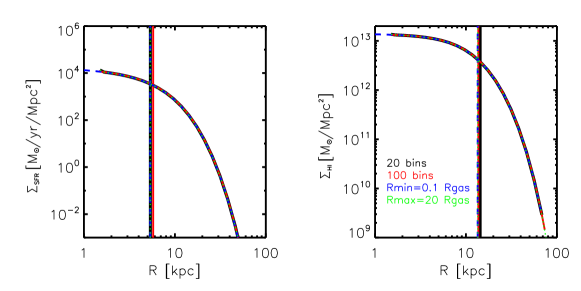
where is the area of each annulus. The annuli are not ‘fixed’ as in e.g. Fu et al. (2010), but recomputed for each star formation episode. We checked that results are not significantly affected by the number and size of the rings. In particular, we carried out test runs using 100 annuli, a larger outer radius (), or a smaller inner radius (), and find little difference in the final properties of galaxies. Fig. 1 shows the surface density profile of the star formation rate and HI for one particular galaxy at . Only results for one of the models described below (the BR06) are shown, but these are similar for all models considered. The vertical lines mark the effective radius, defined as the radius that includes half of the total SFR or half of the HI mass. We find that different choices for the division of the disks in annuli cause less than per cent differences for the sizes of the cold gas disks and stellar disks, for all galaxies above the resolution limit of our simulations. We verify that also the relations between SFR, HI mass, stellar disk sizes and stellar mass are not significantly affected by different choices for the number or the size of the annuli.
In the next subsections, we discuss in detail the four star formation laws used in our study. Their parameters have been chosen to reproduce the galaxy stellar mass function, HI mass function, and H2 mass function (less weight has been given to this observable because of the relevant uncertainties in the CO to H2 conversion) at using the MS . All parameters entering the modelling of other physical processes are kept unchanged with respect to our fiducial model.
2.4.1 The Blitz & Rosolowsky (2006) star formation law (BR06)
This star formation law is based on the relation observed in local galaxies between the ratio of molecular to atomic hydrogen () and the mid-plane pressure acting on the galactic disc () (Blitz & Rosolowsky, 2006). Specifically:
| (17) |
where is the external pressure of molecular clumps. Based on their sample of 14 nearby galaxies, Blitz & Rosolowsky (2006) find ranging between K and K, and values for varying between and . We assume log and , that correspond to the mean values.
The hydrostatic pressure at the mid-plane can be written as follows (Elmegreen, 1989):
| (18) |
where and are the surface density of the cold gas and of the stars in each annulus, and is the ratio between the vertical velocity dispersion of the gas and that of the stellar disk. We assume a constant velocity dispersion for the gaseous disk of (Leroy et al., 2008), while for the stellar disk we follow Lagos et al. (2011b) and assume and , based on observations of nearby disc galaxies (Kregel, van der Kruit & de Grijs, 2002). For pure gaseous disks, Eq. 18 is simplified by setting to zero the stellar surface density.
2.4.2 The Krumholz, McKee & Tumlinson (2009b) star formation law (KMT09)
In a series of papers, Krumholz, McKee & Tumlinson (2008, 2009a, 2009b) developed an analytic model to determine the fraction of molecular hydrogen, within a single atomic-molecular complex, resulting from the balance between dissociation of molecules by interstellar radiation, molecular self-shielding, and formation of molecules on the surface of dust grains. Accounting for the fact that the ratio between the intensity of the dissociating radiation field and the number density of gas in the cold atomic medium that surrounds the molecular part of a cloud depends (weakly) only on metallicity (Wolfire et al., 2003), the molecular to total fraction can be written as:
| (20) |
where,
| (21) |
| (22) |
| (23) |
and
| (24) |
is the surface density of a giant molecular cloud (GMC) on a scale of pc, and is the metallicity of the gas normalized to the solar value (we assume ). Following Krumholz, McKee & Tumlinson (2009b), we assume , where is a ‘clumping factor’ that approaches 1 on scales close to 100 pc, and that we treat as a free parameter of the model. In previous studies, values assumed for this parameter range from (Fu et al., 2010) to (Lagos et al., 2011b). In our case, provides predictions that are in reasonable agreement with data, while larger values tend to under-predict the HI content of massive galaxies. Krumholz, McKee & Tumlinson (2009b) stress that some of the assumptions made in their model break at gas metallicities below roughly 5 per cent solar (). As discussed e.g. in Somerville, Popping & Trager (2015), POP III stars will rapidly enrich the gas to metallicities at high redshift. Following their approach, when computing the molecular fraction, we assume this threshold in case the metallicity of the cold gas is lower. We adopt the same treatment also in the GK11 model and K13 models described below.
As for the efficiency of star formation, we follow Krumholz, McKee & Tumlinson (2009b) and assume:
| (25) |
where is the average surface density of GMCs in Local Group galaxies (Bolatto et al., 2008), and is the typical value found in GMCs of nearby galaxies. We find a better agreement with H2 mass function at when using a slightly larger values for this model parameter: .
2.4.3 The Krumholz (2013) star formation law (K13)
Krumholz (2013) extend the model described in the previous section to the molecule-poor regime (here the typical star formation rate is significantly lower than that found in molecular-rich regions). KMT09 assumes the cold neutral medium (CNM) and warm neutral medium (WDM) are in a two-phase equilibrium. In this case, the ratio between the interstellar radiation field () and the column density of CNM () is a weak function of metallicity. However the equilibrium breaks down in HI-dominated regions. Here, and are calculated as summarized below.
The molecular hydrogen fraction can be written as:
| (26) |
where,
| (27) |
| (28) |
| (29) |
and .
As for the KMT09 model, we assume and use to estimate the molecular fraction when the cold gas metallicity . In the above equations, represents a dimensionless radiation field parameter. Our model adopts a universal initial mass function (IMF) for star formation, both for quiescent episodes and star-bursts. UV photons are primarily emitted by OB stars, and the UV luminosity can be assumed to be proportional to the star formation rate. To estimate , we use the star formation rate integrated over the entire gaseous disk, averaged over the time interval between two subsequent snapshots (this correspond to 20 time-steps of integration) 444 A similar modelling has been adopted in Somerville, Popping & Trager (2015). We note that a more physical expression for the intensity of the interstellar radiation field would be in terms of the surface density of the star formation rate. We have tested, however, that within our semi-analytic framework such alternative expression does not affect significantly our model predictions. Results of our tests are shown in Appendix C.. Specifically, we can write:
| (30) |
and assume for the total SFR of the Milky Way (observational estimates range from to , e.g. Murray & Rahman 2010; Robitaille & Whitney 2010).
is assumed to be the largest between the minimum CNM density in hydrostatic balance and that in two-phase equilibrium:
| (31) |
In particular, the column density of the CNM in two-phase equilibrium can be written as:
| (32) |
while
| (33) |
is the Boltzmann constant, is the maximum temperature of the CNM (Wolfire et al., 2003), and is the thermal pressure at mid-plane (Ostriker, McKee & Leroy, 2010):
| (34) |
In the above equation, is the molecular hydrogen mass after star formation at the last time-step, is the current total cold gas mass, and is the volume density of stars and dark matter. To compute the latter quantity, we assume a NFW profile for dark matter haloes and assign to each halo, at a given redshift and of given mass (), a concentration using the calculator provided by Zhao et al. (2009). Once the halo concentration is known, we can compute the density of dark matter at a given radius. The volume density of stars is computed assuming an exponential profile for the stellar disk and a Jaffe (1983) profile for the stellar bulge. For the stellar disk height, we assume . The other parameters correspond to the velocity dispersion of gas , and a constant .
In the GMC regime, the free fall time of molecular gas is:
| (35) |
Then the star formation efficiency of transforming molecular gas to stars is given by:
| (36) |
2.4.4 The Gnedin & Kravtsov (2011) star formation law (GK11)
Gnedin & Kravtsov (2011) carry out a series of high resolution hydro-simulations including non-equilibrium chemistry and an on-the-fly treatment for radiative transfer. Therefore, their simulations are able to follow the formation and photo-dissociation of molecular hydrogen, and self-shielding in a self-consistent way. Gnedin & Kravtsov provide a fitting function that parametrizes the fraction of molecular hydrogen as a function of the dust-to-gas ratio relative to that of the Milky Way (), the intensity of the radiation field (), and the gas surface density (). In particular:
| (37) |
where is a characteristic surface density of neutral gas at which star formation becomes inefficient.
| (38) |
with:
| (39) |
| (40) |
| (41) |
| (42) |
| (43) |
Following GK11, we use the metallicity of cold gas to get the dust ratio: . For , we assume the same modelling used for the K13 star formation law. We note that the simulations by Gnedin & Kravtsov (2011) were carried out varying from to , and from and . Their fitting formulae given above are not accurate when . We assume to calculate the molecular fraction when the cold gas metallicity .
GK11 also provide the star formation efficiency necessary to fit the observational results in Bigiel et al. (2008) in their simulations:
| (44) |
where is the surface density of cold gas, , and .
3 The influence of different star formation laws on galaxy physical properties
As mentioned in Section 2, we run our models on two high-resolution cosmological simulations: the Millennium Simulation (MS), and the Millennium II (MSII). Our model parameters are calibrated using the MS, and merger trees from the MSII are used to check resolution convergence. The main observables that are used to calibrate our models are: the galaxy stellar mass function, and the HI and mass functions at . A comparison between observational data and predictions from one of our models (BR06) for galaxy clustering in the local Universe has been presented recently in Zoldan et al. (2017).
In this section, we analyse in more detail the differences between the star formation laws considered, and discuss how they affect the general properties of galaxies in our semi-analytic model. Table 3 lists all star formation laws considered in this work and the corresponding parameters.
| Model (color) | Molecular fraction [, ] | Star formation efficiency [, ] | Model parameters | |
|---|---|---|---|---|
| 1. Fiducial (black) | Fixed molecular fraction . | , , | same as in HDLF16 | |
| 2. BR06 (red) | , , | , | ||
| 3. KMT09 (blue) | , , | |||
| if , | ||||
| if | , | |||
| , | ||||
| , | ||||
| 4. K13 (yellow) | ||||
| if , | ||||
| if , , , | , | |||
| , | ||||
| , | ||||
| 5. GK11 (green) | , | |||
| , | ||||
| , | ||||
| , | ||||
| , | ||||
| if , | ||||
| if | , | |||
| , | ||||
| , | ||||
3.1 Differences between H2 star formation laws
As discussed in the previous section, the star formation laws used in this study can be separated in a component given by the calculation of the molecular fraction (or ) and one given by the star formation efficiency .
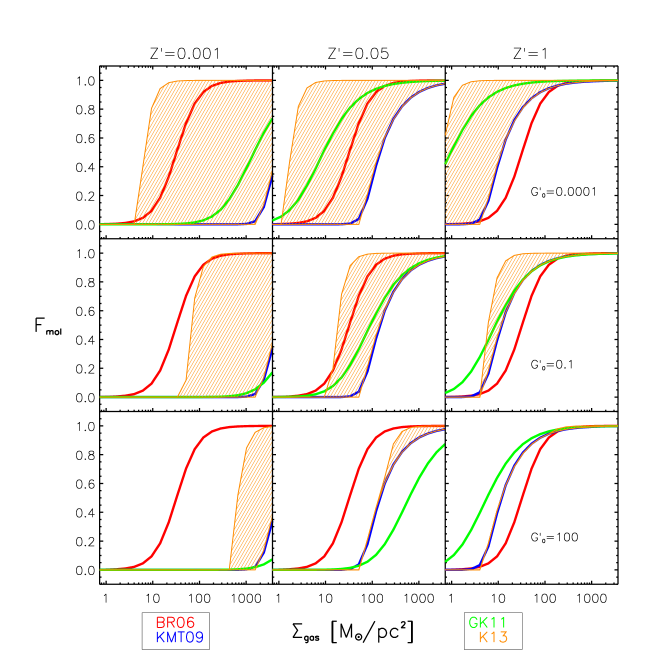
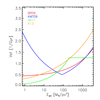
Fig. 2 shows the molecular fraction predicted by the models considered in this study in three bins of interstellar radiation intensities and gas metallicity, as a function of the gas surface density. Lines of different colours correspond to different models, as indicated in the legend. The molecular fraction in BR06 depends only on the disk pressure, so the red curve is the same in each panel. The stellar disk pressure is assumed to be zero for the line shown. Assuming a positive value for the pressure of the stellar disk, BR06 would predict a slightly higher , but this would not affect our conclusions. In the K13 model, the molecular fraction calculation is based on the molecular ratio at last time-step (Equation 34). The shaded region shown in the figure highlights the minimum and maximum value for the molecular fraction, corresponding to the case its value at the previous time-step is (H2-dominated region) or (HI-dominated region) respectively. Since we do not have halo information for K13, we assume and (Krumholz, 2013, see equation 35). In Appendix C, we show that this assumption gives results that are very similar to those obtained using the approach described in Section 2.4.3 to compute .
The predicted molecular fraction differs significantly among the models considered. For a metal poor galaxy with little star formation and therefore low interstellar radiation (this would correspond to the initial phases of galaxy formation), BR06 and K13 predict higher molecular fraction than GK11 and KMT09 (top left panel). At fixed radiation intensity, an increase of the gas metallicity corresponds to an increase of the molecular fraction predicted by the all models but BR06. This is because a higher gas metallicity corresponds to a larger dust-to-gas ratios, which boosts the formation of hydrogen molecules. For the highest values of gas metallicity considered (top right panel) the GK11 model produces the highest molecular fraction, BR06 the lowest. When the interstellar radiation increases (from top to bottom rows) hydrogen molecules are dissociated more easily and so the molecular fraction, at fixed metallicity and gas surface density, decreases. In particular, the GK11, KMT09 and K13 models predict a very low molecular fraction for the lowest metallicity and largest radiation intensity considered (bottom left panel). As metallicity in cold gas increases, GK11 predicts more molecular gas than the other models. As expected by construction, in H2-dominated region, K13 gives similar molecular fraction to KMT09. For metal-rich galaxies (right column), GK11 predicts more molecular gas than the other models, particularly at low surface densities. The lowest molecular fractions are instead predicted by the BR06 model.
Fig. 3 shows the star formation efficiency corresponding to the four star formation laws implemented, as a function of the gas surface density (see third column of Table 3). BR06 and K13 predict an increasing star formation efficiency with increasing surface density of cold gas. GK11 predicts a monotonic increase of the star formation efficiency up to gas surface density and then a flattening. Finally, the KMT09 model predicts a decreasing star formation efficiency up to . For higher values of the gas surface density, the predicted star formation efficiency increases and is very close to that predicted by the BR06 model. It is interesting to see if these different predictions translate into a correlation between the star formation rate surface density and gas surface density that is in agreement with the latest observations.
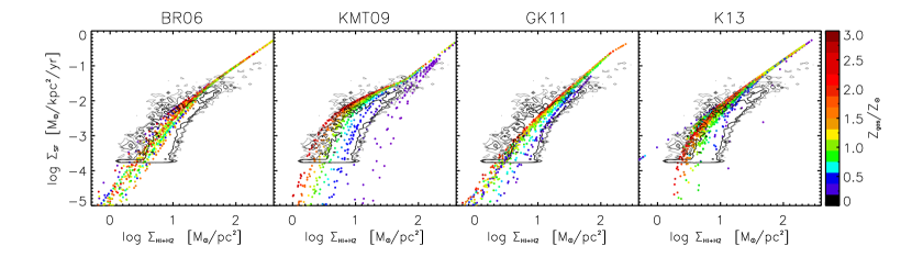
Fig 4 shows the surface density of star formation rate against the surface density of neutral gas . We select galaxies in MSII at redshift and compare with observational estimates compiled in Bigiel et al. (2010). Dots correspond to the surface density of star formation rate and neutral gas in each annulus of model galaxies. Their colour indicates their cold gas metallicity. The figure shows that all four star formation laws considered in our work reproduce observations relatively well. The dependence on metallicity for the KMT09 model is obvious. In the GK11 and K13 models, the star formation rate depends also on the radiation intensity and the metallicity dependence is weaker. Somerville, Popping & Trager (2015) present their predicted relation in their Fig. 6. They find a clear metallicity dependence also for their prescription where H2 is determined by the pressure of the interstellar medium, while for our BR06 model we do not find a clear dependence on metallicity. We believe that the reason is the different chemical enrichment models. Somerville, Popping & Trager (2015) use a fixed yield parameter, which naturally leads to a tight relation between stellar surface density and cold gas metallicity. In contrast, our model includes a detailed recycling and the metallicity of the cold gas and the disk pressure are not highly correlated for our simulated galaxies.
3.2 The growth of galaxies in models with different star formation laws
To show the influence of different star formation laws on the star formation history of model galaxies, we select a sample of central model galaxies in our fiducial model and compare their history to that of the same galaxies modelled using the different star formation laws considered. In particular, we randomly select galaxies in three stellar mass bins in the fiducial model555The final stellar masses are not significantly different in the other models, as shown in Fig. 5: . For each galaxy, we trace back in time its main progenitor (the most massive progenitor at each node of the galaxy merger tree). Fig. 5 compares the average growth histories of these galaxies. For this analysis, we use our runs based on the MSII. The HI and H2 masses in the fiducial model are obtained assuming a constant molecular ratio .
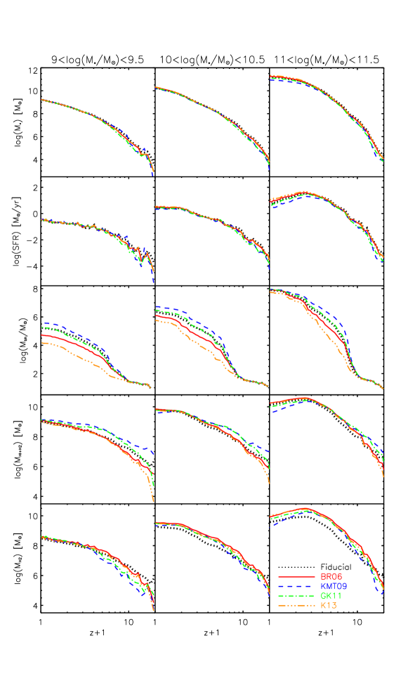
Let us focus first on galaxies in the lowest mass bin considered ( at , the left column in Fig. 5). In all H2-based star formation laws considered, star formation starts with lower rates than that in our fiducial model. This happens because the amount of molecular hydrogen at high redshift is lower than that in the fiducial model (see bottom left panel). In addition, star formation in the fiducial model takes place only after the gas surface density is above a critical value, so most galaxies in this model form stars intermittently (this does not show up because Fig. 5 shows a mean for a sample of galaxies): once enough gas is accumulated, stars can form at a rate that is higher than that predicted by our H2-based star formation laws. Then for one or a few subsequent snapshots, the star formation rate is again negligible until the gas surface densities again overcomes the critical value. In contrast, for the H2-based models considered, star formation at early times is low but continuous for most of the galaxies. Predictions from the BR06 and K13 models are very close to each other while the slowest evolution is found for the KMT09 model. The cold gas masses of low mass galaxies are different between models at early times. KMT09 and GK11 predict more cold gas than fiducial model, while BR06 and K13 predict the lowest cold gas mass. All models converge to very similar values at for stellar mass and SFR, within a factor of . The mass of molecular hydrogen converges only at . The average mass of cold gas remains different until present (at the mass of cold gas predicted by KMT09 model is about times of that predicted by K13 model).
For the other two stellar mass bins considered (middle and right columns in Fig. 5), the trends are the same, but there are larger differences at low redshift. In particular, for the most massive bin considered, the amount of molecular gas in the fiducial model stays almost constant at redshift , while it decreases for the other models. This is particularly evident for the KMT09 model and is due to the fact that the black hole mass is larger and therefore the AGN feedback is more efficient. For the same reason, both the star formation rate and the stellar mass predicted by this model are below those from the other ones over the same redshift interval.
As explained in Section 2.3, black holes grow through smooth accretion of hot gas and accretion of cold gas during galaxy mergers. Galaxies in the fiducial model have more cold gas than those in BR06 and K13 at early times, thus the fiducial model predicts more massive black holes. The KMT09 and GK11 models predict even more massive black holes because, when mergers take place there are significant amounts of cold gas available that has not yet been used to form stars.
3.3 The galaxy stellar mass function
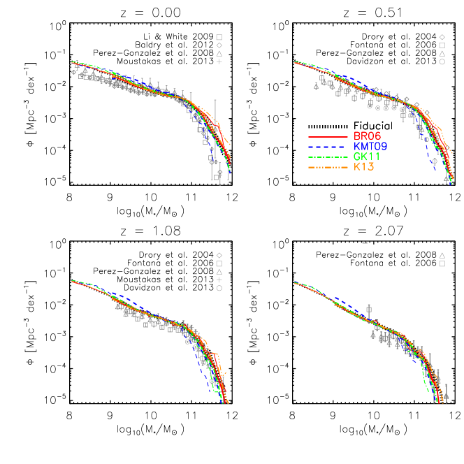
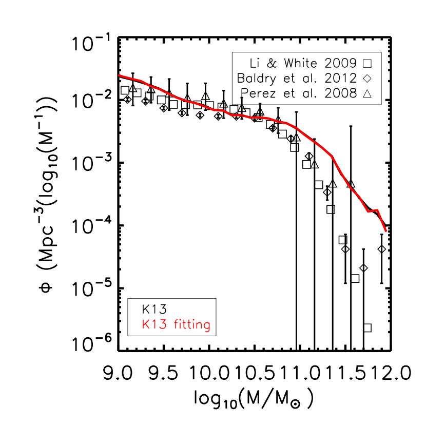
Fig. 6 shows the galaxy stellar mass functions predicted by the different models considered in our study and compare them to observational measurements at different cosmic epochs. In this figure (and in all the following), thicker lines are used for the MS (about of the entire volume) and thinner lines for the MSII (about of the volume), while different colours correspond to different star formation laws. We note that the stellar mass function corresponding to our fiducial model run on the MS at , shows a higher number density of massive galaxies with respect to the results published in HDLF16. We verified that this is due to our updated black hole model (see Appendix B).
Predictions from all models are close to those obtained from our fiducial model, at all redshifts considered. The KMT09 and GK11 models tend to predict lower number densities for galaxies above the knee of the mass function, particularly at higher redshift. This is due to the fact that black holes in KMT09 and GK11 are slightly more massive than in the fiducial model. In contrast, black holes in the BR06 and K13 models are less massive than those in the fiducial model for the MSII. As a consequence, the BR06 and K13 models predict more massive galaxies above the knee of the mass function with respect to the fiducial model. We have not been able to find one unique parametrization for the black hole seeds, or modification of the black hole model, that are able to provide a good convergence between the MS and MSII for all four star formation laws in our study. Below the knee of the mass function, model predictions are very close to each other with only the KMT09 model run on the MS predicting slightly larger number densities. The predictions from the same model based on the MSII are very close to those obtained from the other models, showing this is largely a resolution effect.
3.4 The HI and H2 mass functions
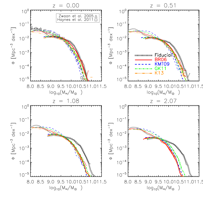
Fig. 6 shows that the galaxy stellar mass function is complete down to for the MS and for the MSII. Only galaxies above these limits are considered in this section.
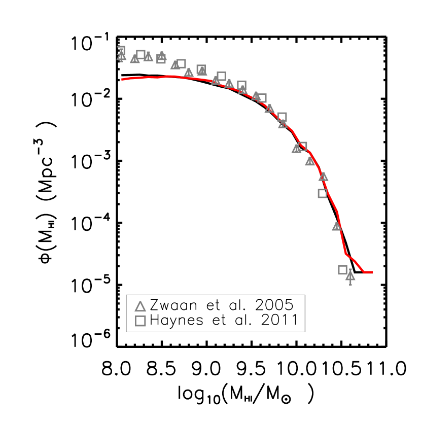
Fig. 7 shows the predicted HI mass function from all models used in this study. For our fiducial model, we assume a constant molecular fraction of to estimate the amount of HI from the total cold gas associated with model galaxies. The grey symbols correspond to observational data by Zwaan et al. (2005, triangles) and Haynes et al. (2011, squares).
All models agree relatively well with observations at , by construction (we tune the free parameters listed in Table 3 so as to obtain a good agreement with the HI and H2 mass function at ). Comparing results based on the MS and MSII, the figure shows that resolution does not affect significantly the number densities of galaxies with HI mass above at all redshifts. Below this limit, the number density predicted from all models run on the MS are significantly below those obtained using the higher resolution simulation. The fiducial model tends to predict higher number densities of HI rich galaxies, particularly at higher redshift. This is due to the fact that all H2-based star formation laws predict increasing molecular fractions with increasing redshift, in qualitative agreement with what inferred from observational data (e.g. Popping et al., 2015).
While it is true that predictions from the other models are relatively close to each other, the figure shows that there are some non negligible differences between them. In particular, the KMT09 model tend to predict the lowest number densities for galaxies above the knee, and the highest number densities for HI masses in the range . This is because massive galaxies in the KMT09 model tend to have more massive black holes than in other models so that radio mode AGN feedback is stronger. In the same model, low mass galaxies tend to have lower star formation rates at high redshift and are therefore left with more cold gas at low redshift (see Fig. 5). The BR06 model has the opposite behaviour, predicting the largest number densities for galaxies above the knee (if we exclude the fiducial model) and the lowest below. The differences between the models tend to decrease with increasing redshift: at all models are very close to each other with only the GK11 model being offset towards slightly higher number densities.
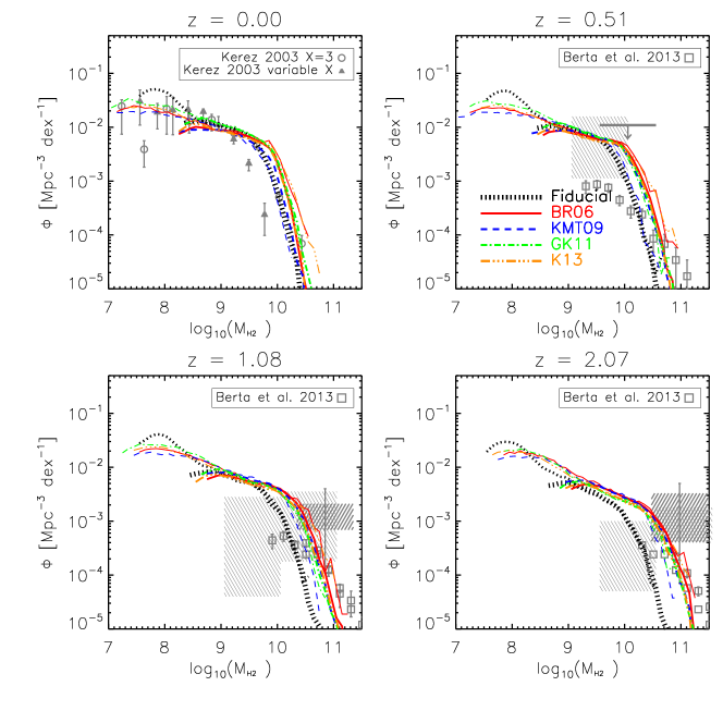
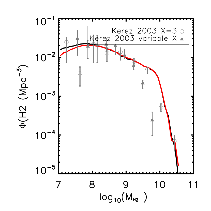
Fig. 8 shows the H2 mass function from redshift to . The observational measurements at are based on the CO luminosity function by Keres, Yun & Young (2003), and assume a constant CO/H2 conversion factor or a variable one (Obreschkow & Rawlings, 2009b). All models over-predict the number density of galaxies with log when considering a variable CO/H2 conversion factor. Results based on the fiducial and KMT09 model are consistent with measurements based on a constant conversion factor. The other models tend to predict more H2 at the high mass end. The trend is the same at higher redshift. Here, we compare our model predictions with estimates by Berta et al. (2013). These include only main sequence galaxies and are based on a combination of PACS far-infrared and GOODS-HERSCHEL data. The molecular mass is estimated from the star formation rate, measured by using both far-infrared and ultra-violet photometry. All models tend to over-predict significantly the number densities of galaxies with H2 below . This comparison should, however, be considered with caution as measurements are based on an incomplete sample and an indirect estimate of the molecular gas mass. We also include, for comparisons, results of blind CO surveys (Walter et al., 2014; Decarli et al., 2016). These are shown as shaded regions in Fig. 8.
For the H2 mass function, resolution starts playing a role at at , but the resolution limit increases significantly with redshift: at the runs based on the MS become incomplete at H2 masses . Resolution also has an effect for the H2 richest galaxies for the KMT09, BR06, and K13 models. We find that this is due to the fact that black holes start forming earlier in higher resolution runs, which affects the AGN feedback and therefore the amount of gas in the most massive galaxies.
To summarize, all star formation laws we consider are able to reproduce the observed stellar mass function, HI mass function, and H2 mass function. We obtain a good convergence between MS and MSII at for the galaxy stellar mass function, for the HI mass function, and from to for the H2 mass function. As explained above, model predictions do not converge for the massive end of the galaxy stellar mass function and H2 mass function, and this is due to a different effect of AGN feedback (see Appendix B). We do not find significant differences between predictions based on different star formation laws. Based on these results, we argue that it is difficult to discriminate among different star formation laws using only these statistics, even when pushing the redshift range up to , and including HI and H2 mass as low as . Indeed, the systematic differences we find between different models are very small. Our results also indicate that there are significant differences between results obtained by post-processing model outputs and those based on the same physical model but adopting an implicit molecular based star formation law.
4 Scaling relations
In this section, we show scaling relations between the galaxy stellar mass and other physical properties related directly or indirectly to the amount of gas associated with galaxies, at different cosmic epochs. In order to increase the dynamic range in stellar mass considered and the statistics, we take advantage of both the MS and the MSII. In particular, unless otherwise stated, we use all galaxies with from the former simulation, and all galaxies with from the latter. As shown in the previous section, and discussed in detail in Appendix B, the convergence between the two simulations is good, and we checked that this is the case also for the scaling relations as discussed below.
4.1 Atomic and molecular hydrogen content
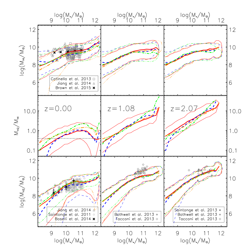
We begin with a comparison between model predictions and observational data for the amount of atomic and molecular hydrogen associated with galaxies of different stellar mass, and at different cosmic epochs. This is shown in Fig. 9, for all models used in our study. The top panels show the predicted relation between the HI mass and the galaxy stellar mass, and compare model predictions with observational estimates of local galaxies from the GASS survey (Catinella et al., 2013, squares) and from a smaller sample (32 galaxies) with HI measured from ALFALFA (Jiang et al., 2015, triangles). The former survey is based on a mass-selected sample of galaxies with , while the sample by Jiang et al. (2015) includes only star forming nearby galaxies, and is therefore biased towards larger HI masses. Brown et al. (2015, black multiplication sign) provide average results of NUV-detected galaxies from ALFALFA. Contours show the distribution of model galaxies indicating the region that encloses per cent of the galaxies in each galaxy stellar mass bin considered. All models predict a similar and rather large scatter, with results consistent with observational measurements at for galaxies with stellar mass between and . For lower mass galaxies, all models tend to predict lower HI masses than observational estimates. This is in part due to the fact that observed galaxies in this mass range are star forming. If we select star forming galaxies () from the BR06 model, the median mass of HI is dex higher (but still lower than data) than that obtained by considering all model galaxies. The relation between HI and stellar mass (as well as the amplitude of the scatter) evolves very little as a function of cosmic time.
The middle panels of Fig. 9 show the molecular-to-atomic ratio as a function of the galaxy stellar mass at different redshifts. At , the ratio tends to flatten for galaxy masses larger than and its median value is not much larger than the canonical that is typically adopted to post-process models (shown as the dotted line in the left-middle panel) that do not include an explicit partition of the cold gas into its atomic and molecular components. For lower galaxy stellar masses, the molecular-to-atomic ratio tends to decrease with decreasing galaxy mass due to their decreasing gas surface density. The BR06 and KMT09 models predict the lowest molecular-to-atomic ratios at , while the GK11 model the highest. At higher redshifts, the relation becomes steeper also at the most massive end, differences between the different models become less significant, and the overall molecular-to-atomic ratio tends to increase at any value of the galaxy stellar mass. Specifically, galaxies with stellar mass have a molecular-to-atomic ratio of about at , at , and at . For galaxies with stellar mass , the molecular-to-atomic gas ratio varies from at to at . The evolution of the molecular ratio is caused by the evolution of the size-mass relation: galaxies at high redshift have smaller size and higher surface density than their counterparts at low redshift. The relations shown in the middle panel clarify that a simple post-processing adopting a constant molecular-to-atomic ratio is a poor description of what is expected on the basis of more sophisticated models. One could improve the calculations by assuming a molecular-to-atomic ratio that varies as a function of redshift and galaxy stellar mass. We note, however, that there is a relatively large scatter in the predicted relations that would not be accounted for.
The bottom panels of Fig. 9 shows, the molecular hydrogen mass as a function of galaxy stellar mass. Symbols correspond to different observational measurements. At , filled circles are used for data from the COLDGAS survey (Saintonge et al., 2011). These are based on CO(1-0) line measurements and assume to convert CO luminosities in H2 masses. Data from Jiang et al. (2015, open triangles) include only main sequence star forming galaxies, are based on CO(2-1) lines, and assume . Boselli et al. (2014) provide mean values and standard deviations of late-type galaxies, classified by morphology and selected from the Herschel Reference Survey, with a constant conversion factor . The samples observed at higher redshift are less homogeneous and likely biased. Measurements by Saintonge et al. (2013, dots) are for a sample of 17 lensed galaxies with measurements based on CO(3-2) lines and metallicity-dependent conversion factors. Data from Tacconi et al. (2013, diamonds) are for a sample of 52 star forming galaxies with measurements based on CO(3-2) lines and assuming . Galaxies from their sample cover the redshift range from to ; we plot all those below in the middle panel and all those above in the right panel. Bothwell et al. (2013) give data for 32 sub-millimetre galaxies and assume . As for the top panels, thick lines show the median relations predicted from the different star formation laws considered in our paper, while the thin contours mark the region that encloses per cent of the galaxies in each stellar mass bin. At , observational data are close to the median relations obtained for the different models. The data by Jiang et al. (2015), as well as most of those considered at higher redshift, tend to be above the median relations although all within the predicted scatter. We verify that this is still the case even when considering only main sequence star forming galaxies at . Similar results were found by Popping, Somerville & Trager (2014).
4.2 Galaxy stellar mass - cold gas metallicity relation
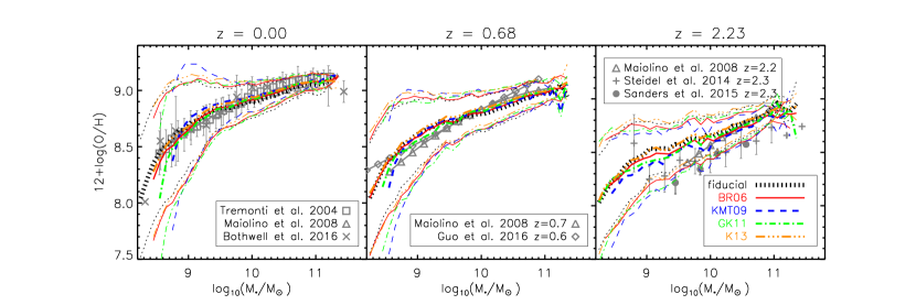
Three of the star formation laws used in this study include an explicit dependence on the metallicity of the cold gas component. Therefore, it is important to verify that the observed correlation between the galaxy stellar mass and the gas metallicity is reproduced. Fig. 10 shows the oxygen abundance of cold gas666We remove helium () from cold gas to get the abundance of Hydrogen, whereas HDLF16 did not. Therefore our results for the fiducial model are different from those of the FIRE model in Fig. 6 of HDLF16. from redshift to predicted by all models considered in this study, and compares model predictions with different observational measurements. For this figure, we select star forming galaxies (, where is the Hubble time), with no significant AGN (), and with gas fraction . We used this selection in an attempt to mimic that of the observational samples, that mainly include star forming galaxies.
Model results are in quite good agreement with data and predictions from the different models are relatively close to each other. At , all models tend to over-predict the estimated metallicities compared to observational measurements by Steidel et al. (2014) and Sanders et al. (2015). Our model predictions are, instead, very close to the measurements for galaxies more massive than by Maiolino et al. (2008). Fig. 10 shows that the GK11 and KMT09 model predict slightly lower gas metallicities for low mass galaxies at the highest redshift shown. The mass-metallicity relation shown in Fig. 10 extends the dynamic range in stellar mass shown in HDLF16, where we also used a slightly different selection for model galaxies. While we defer to a future study a more detailed comparison with observational data at the low-mass end, we note that our model is the only published one that reproduces the estimated evolution of the mass-metallicity relation up to (and up to for the most massive galaxies). As discussed in Somerville, Popping & Trager (e.g. 2015), this is an important prerequisite for models that are based on metallicity dependent star formation laws.
4.3 Star forming sequence
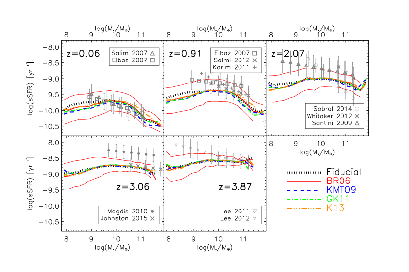
Fig. 11 shows the specific star formation rate (sSFR) as a function of galaxy stellar mass, from redshift to . Only model galaxies with sSFR are used for this analysis. Gray symbols correspond to different observational measurements based on Hα (Elbaz et al., 2007; Sobral et al., 2014), UV (Salim et al., 2007; Johnston et al., 2015), UV+IR (Salmi et al., 2012; Santini et al., 2009), and FUV (Magdis et al., 2010; Lee et al., 2011, 2012). Symbols and error bars correspond to the best fitting and standard deviation given in Speagle et al. (2014). All derived stellar masses are converted to a Chabrier IMF (dividing by in the case of a Kroupa IMF, and in case of a Salpeter IMF). We have also converted the different estimates of the star formation rates to a Chabrier IMF using the population synthesis model by Bruzual & Charlot (2003).
All models predict decreasing sSFRs with decreasing redshift at fixed stellar mass, a trend that is consistent with that observed. Model predictions agree relatively well with observational measurements up to for galaxies more massive than . At lower masses, data suggests a monotonic increase of the sSFR with decreasing galaxy stellar mass while the predicted relation are relatively flat. This trend is driven by central galaxies whose sSFR decreases slightly with decreasing stellar mass, while satellite galaxies are characterized by a flat sSFR - stellar relation. For galaxies at , star formation rates are under-estimated in models, especially for low mass galaxies. The same problem was pointed out in HDLF16 and is shared by other published galaxy formation models (Fu et al., 2012; Weinmann et al., 2012; Mitchell et al., 2014; Somerville, Popping & Trager, 2015; Henriques et al., 2015). Although there are still large uncertainties on the measured sSFRs, particularly at high redshift, the lack of actively star forming galaxies (or, in other words, the excess of passive galaxies) at high redshift still represents an important challenge for theoretical models of galaxy formation. Previous studies argued that suppressing the star formation efficiency at early times (by using some form of pre-heating or ad hoc tuned ejection and re-incorporation rates of gas) so as to post-pone it to lower redshift could alleviate the problem (see e.g. White, Somerville & Ferguson, 2015; Hirschmann, De Lucia & Fontanot, 2016). A metallicity dependent star formation law is expected to work in the same direction. However, surprisingly, all different star formation laws considered in our study predict a very similar relation between sSFR and galaxy stellar mass, at all redshifts considered. This is because different star formation laws predict similar star formation rates for ’high’ surface density : the majority of galaxies in our model have gas surface density above this value. Previous studies (Lagos et al., 2011b; Somerville, Popping & Trager, 2015) also find that the different star formation laws have little effect for active galaxies.
4.4 Disk sizes
In this section, we show model predictions for the radii of the HI and stellar components, as well as for the star forming radius. We define as effective radius the radius that encloses half of the total SFR, HI, or stellar mass, and assume exponential surface density profiles for both the stellar and the gaseous disks (see equation 6). We also assume that the bulge density profile is well described by a Jaffe law (Jaffe, 1983). As discussed in Section 2.2, the scale lengths of the gaseous and stellar disks are determined assuming conservation of the specific angular momentum. The star forming radius is instead measured by integrating star formation over 20 annuli (see Section 2.4).
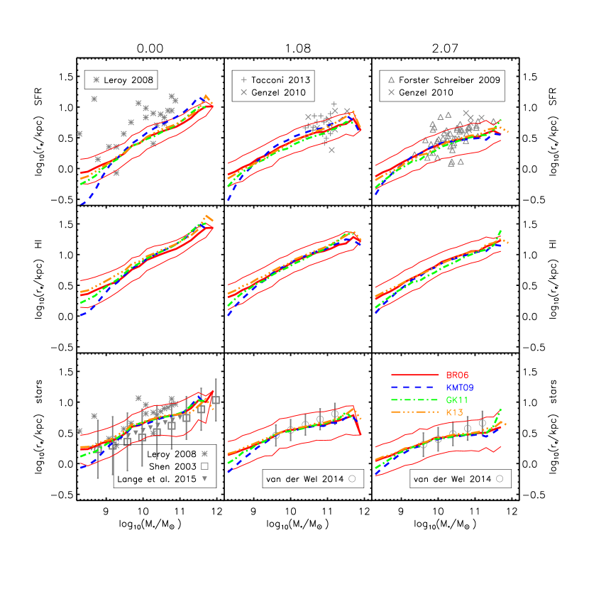
Fig. 12 compares model predictions with observational data at different redshifts. We only select disk dominated galaxies (), with gas fraction , and specific star formation rate s to make fair comparisons with observations. The data shown in the top panels of Fig. 12 correspond to the half-light radii estimates from the PHIBSS survey (Tacconi et al., 2013, based on CO(3-2) lines), from SINS (Förster Schreiber et al., 2009, based on Hα), and Genzel et al. (2010) (a combination of Davis et al. (2007); Noeske et al. (2007); Erb et al. (2006) based on a combination of Hα, UV, and CO maps). The sizes from Leroy et al. (2008) correspond to the scale lengths of exponential fits to the stellar and star formation surface density, and are derived from K-band and FUV+24m, respectively. The estimated scale lengths are multiplied by a factor to convert them in a half mass radius. The stellar radii shown in the bottom panels correspond to the half-light radii measured from CANDLES and 3D-HST (van der Wel et al., 2014), from GAMA Lange et al. (2015), and from SDSS galaxies (Shen et al., 2003).
For galaxies with fixed stellar mass, the effective HI and SFR radii evolve little from redshift to present. The ratio between the SFR radius and the HI radius of a typical galaxy with at is times that of a galaxy with the same stellar mass at . In contrast, the stellar size of the same galaxy at is times of that at . At redshift , the SFR and stellar effective radii are similar, while at , the stellar radii are nearly times the star forming radii. Available data, however, suggest that the star forming radii are larger than the stellar radii at . At all redshift, HI size is times of SFR size. Note that the stellar size-mass relation of Leroy et al. (2008) differs from that by Shen et al. (2003) and Lange et al. (2015) because of the different selection criteria and different measurements of the half mass radius. Leroy et al. (2008) select star forming galaxies and measured the half mass radius by fitting exponential profiles to the stellar surface density, as we do. Shen et al. (2003); Lange et al. (2015) measured half mass radius of Sérsic fits and selected late-type galaxies with Sérsic index .
The predicted stellar radii are comparable with observational estimates at all redshifts considered. The star forming radii are under-estimated in the models by about dex at , but in relatively good agreement with data at higher redshift. The four star formation laws used in our study predict very similar size-mass relation, at all redshifts considered. This is expected: in our model, disk sizes are calculated using the angular momentum of the accreted cold gas. As we already discussed, different star formation laws predict very similar star formation histories. So the consumption and accretion histories of cold gas are also very similar. Our results are consistent with those by Popping, Somerville & Trager (2014) who compared star forming radii with a model including prescriptions similar to our BR06 and GK11 models.
5 Cosmic evolution of neutral hydrogen
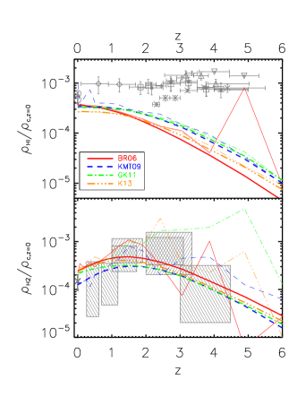
Fig. 13 shows the evolution of the cosmic density of HI (top panel) and H2 (bottom panel). As shown in Fig. 6, our galaxy stellar mass functions are complete down to when run on MSII. The thick lines shown in Fig. 13 correspond to the density of HI and H2 obtained by summing up all galaxies above the completeness limit of the MSII in the simulation box. Thin lines correspond to densities estimated by fitting777We perform the fit considering the mass range between the peak of the mass function and the maximum mass. the predicted HI and H2 mass functions with a Schechter (1976) distribution:
| (45) |
, and extrapolating model predictions towards infinite low mass. The resulting cosmic density is:
| (46) |
The relatively small size of the box and limited dynamic range in masses lead to a very noisy behaviour of model predictions, particularly for the cosmic density of molecular hydrogen.
We find that all the star formation laws considered in our work predict a monotonic decrease of the HI cosmic density with increasing redshift. The BR06 model predicts the most rapid evolution of the HI density while the GK11 and KMT09 the slowest. A similar trend was found by Popping, Somerville & Trager (2014). This work, as well as Lagos et al. (2011a), predict however a mild increase of the HI density between present and , and then a decrease towards higher redshift. We believe this is due to an excess of galaxies in the HI mass range combined with a faster evolution of the HI mass function at higher redshift in these models with respect to our predictions (compare e.g. Fig. 7 in Popping, Somerville & Trager 2014 and Fig. 8 in Lagos et al. 2011a with our Fig. 7). In the top panel of Fig. 13, we add observational measurements by Zwaan et al. (2005) and Martin et al. (2010) at , and measurements inferred from damped Ly systems (DLAs) at higher redshifts (Péroux et al., 2005; Rao, Turnshek & Nestor, 2006; Guimarães et al., 2009; Prochaska & Wolfe, 2009; Zafar et al., 2013; Noterdaeme et al., 2012; Crighton et al., 2015). While our extrapolated estimates using KMT09 are closer to local estimates (these are also based on fitting the observed HI mass function and extrapolating it to lower masses), all models under-predict the cosmic density of HI at higher redshift. The comparison with DLAs should, however, be interpreted with caution. In fact, HI is attached to galaxies in our model while the nature of DLAs and their relationship with galaxies remains unclear. In addition, low mass galaxies, which are not well resolved in our simulation, are gas rich and their contribution could be important at high redshift(Lagos et al., 2011a).
In the bottom panel of Fig. 13, our predicted cosmic density evolution of molecular hydrogen is compared with measurements by Keres, Yun & Young (2003) at and estimates based on blind CO surveys at higher redshifts (Walter et al., 2014; Decarli et al., 2016). The local estimate of the cosmic density of molecular hydrogen is obtained by fitting the observed mass distribution and extrapolating towards lower masses, as we do for the thin lines. A constant conversion factor () is assumed in this case. The higher redshift estimates are obtained by summing all observed galaxies and assuming . All models predict a mild increase of the H2 cosmic density between and , followed by a somewhat more rapid decrease of the molecular hydrogen density towards higher redshift. These trends are in qualitative agreement with the estimated behaviour although uncertainties are still very large. Our model predictions are in qualitative agreement with those by Popping, Somerville & Trager (2014) and Lagos et al. (2011a). The latter study, however, predicts a much higher peak for the H2 cosmic density at and a larger difference between prediction based on different star formation laws.
6 Discussion
6.1 Comparison with previous work
In the last years, a number of semi-analytic models have been improved to account for H2-based star formation laws. In particular, Fu et al. (2010), Lagos et al. (2011b), and Somerville, Popping & Trager (2015) implement prescriptions for molecular gas formation processes in three independently developed semi-analytic models, and test the influence of different star formation laws. All groups discuss scenarios where the H2 is determined by the pressure of the inter-stellar medium (our BR06 model), or by the analytic calculations by Krumholz, McKee & Tumlinson (2008, 2009a, 2009b, our KMT09 model). In addition, Somerville, Popping & Trager (2015) include a star formation law based on the simulations presented in Gnedin & Kravtsov (2011) as we do for our GK11 model.
These groups use different approaches for the calibration of models: Fu et al. (2010) re-tune their AGN and stellar feedback parameters, as well as the free parameters entering the adopted star formation laws, to reproduce the galaxy stellar mass function, HI, and H2 mass functions at . Lagos et al. (2011b) choose the parameters in the modified star formation laws to fit the observed relation between the surface density of star formation and surface density of gas in nearby galaxies. All other parameters are left unchanged. Somerville, Popping & Trager (2015) use an approach closer to that adopted by Fu et al. (2010), and re-tune both the parameters entering the star formation laws and those related to other physical processes to reproduce the galaxy stellar mass function, the total gas fractions as a function of galaxy stellar mass, and the normalization of the relation between stellar metallicity and galaxy mass, all at .
In our case, we only modify the parameters entering the star formation laws and leave unchanged all parameters entering additional prescriptions (e.g. stellar and/or AGN feedback). As we discuss in Sections 2.2 and 2.3, we update some prescriptions with respect to the original model presented in HDLF16, but these updates have only a marginal effect on the physical properties of our model galaxies. Some of the previous studies (Fu et al., 2012; Somerville, Popping & Trager, 2015) consider separately the effect of the prescriptions adopted to partition cold gas into its atomic and molecular components, and those for the conversion of molecular gas in stars. In this study we do not attempt to separate the effect of these two ingredients.
Our model belongs to the same family of models used by Fu and collaborators, but differs from the model used in their study in a number of important aspects. In particular, as discussed in Section 2.1, our model includes a sophisticated chemical enrichment scheme that allows us to follow the non instantaneous recycling of gas, energy and different metal species into the inter-stellar medium. This is the first time H2-based star formation laws are implemented in a model accounting for non-instantaneous recycling. This is particularly relevant for prescriptions that depend explicitly on the gas metallicity (e.g. KMT09, GK11, and K13 models), because an instantaneous recycling approximation could lead to a too efficient enrichment of the galaxies interstellar medium. Another important success of our model lies in the relatively good agreement we find between model predictions and the observed evolution of the relation between galaxy stellar mass and gas metallicity (see discussion in Section 4.2). This is of course an important prerequisite for the prescriptions that use metallicity of the interstellar medium to estimate the H2 molecular fractions. None of the previous models satisfy this requirement: Fu et al. (2012, see their Fig. 3) show that, at least in some of their models, there is significant evolution of the gaseous phase metallicity, at fixed galaxy mass. The relation between galaxy stellar mass and metallicity, however, tends to be too flat compared to observational estimates, and only one of their models (i.e. that based on the Krumholz et al. calculations) is in relatively good agreement with measurements at . In contrast, all models considered in Somerville, Popping & Trager (2015) predict a mass-metallicity relation that is steeper than observed, with very little evolution as a function of redshift. Lagos et al. (2012) show predictions for the relationship between gas metallicity and B-band luminosity, but only at . The evolution of the mass-metallicity relation based on the model discussed in Gonzalez-Perez et al. (2014, this is essentially an update of the Lagos et al. model to the WMAP7 cosmology) is shown in Guo et al. (2016, see their Fig. 12). Also in this case, very little evolution is found as a function of redshift, and the relation is steeper than observational estimates. Our Fig. 10 shows that all models considered in this paper predict a mass-metallicity relation that is in very good agreement with observational estimates at , all the way down to the resolution limit of the Millennium II simulation. The predicted evolution as a function of redshift is also in good agreement with data at , and up to for galaxies more massive than . Less massive galaxies tend to have higher cold phase metallicities in the models than in the data at the highest redshift considered (). We note, however, that observational samples at this redshift are still sparse and likely strongly biased.
The implementation of H2 based star formation laws generally includes an explicit dependence on the sizes of the galaxies (in particular of the disk, and of its star forming region). Therefore, an additional important requirement is that the adopted model reproduces observational measurements for the star forming disks. We show in Section 4.4 that our model satisfies this requirement too. Similar agreement with observational estimates of disk sizes has been discussed in Popping, Somerville & Trager (2014) for two of the models considered in Somerville, Popping & Trager (2015). Lagos et al. (2011b) fail to reproduce the measured relation between the optical size and the luminosity of galaxies in the local Universe (see their Fig. D3). Fu et al. (2010) do not discuss the sizes of their model galaxies with respect to observational constraints. Finally, we note that our reference model does reproduce the observed evolution of the galaxy stellar mass function. As discussed in HDLF16, this is due to the implementation of an updated stellar feedback scheme in which large amounts of the baryons are ‘ejected’ and unavailable for cooling at high redshift, and the gas ejection rate decrease significantly with cosmic time. Lagos et al. (2011b) also reproduce the stellar mass function up to (Gonzalez-Perez et al., 2014, Fig. A7). Both the models discussed in Fu et al. (2012, their Fig. 7) and in Somerville, Popping & Trager (2015, their Fig. 7) exhibit the well known excess of galaxies with intermediate to low mass galaxies at high redshift.
6.2 Can we discriminate among different star formation laws?
In agreement with previous studies, we find that modifying the star formation laws does not have significant impact on the global properties of model galaxies and their distributions. As discussed in Lagos et al. (2011b); Somerville, Popping & Trager (2015) , as well as works based on hydro-simulations (Schaye et al., 2010; Haas et al., 2013), this can be understood as a result of self-regulation of star formation: if less stars are formed, stellar feedback is less efficient in depleting the galaxy inter-stellar medium and more gas is then available for subsequent star formation. Vice versa, if star formation is more efficient, significant amounts of gas are ejected and subsequent star formation is less efficient. The net result of this self-regulation is that the average star formation histories (as well as the mass accretion histories and other physical properties of galaxies) are not significantly altered when different star formation laws are considered.
In agreement with previous papers, we find that the number densities of galaxies below the knee of the mass function are insensitive to the adopted star formation laws in the redshift range . At variance with previous models, we find significant differences for the number densities of the most massive galaxies in models with different star formation laws. We find this is caused by the fact that differences in the amount of gas available at high redshift lead to a different growth history for the black holes, and therefore to a different importance of radio mode AGN feedback. The effect is particularly strong for metallicity dependent star formation laws that lead to higher accretion rates onto the central black holes at higher redshift (see Section 3.2). Somerville, Popping & Trager (2015) use a black hole model that limits the black hole mass to the observed BH-bulge relation (Hirschmann et al., 2012). The available excess cold gas in their GKfid model will, therefore, not lead to excessively massive black holes. Fu et al. (2010) assume that star formation rates depend on the surface density of total cold gas, instead of the molecular gas, when . In this way, their model based on the Krumholz et al. calculations predicts star formation rates comparable to those obtained using the alternative prescriptions based on pressure of the ISM at early times. This leads to very similar black hole masses at late times when adopting different star formation laws. The model of Lagos et al. (2011b) with BR06 and KMT09 also leads to a large amount of cold gas reservoir in galaxies at high redshift. But this cold gas contributes to star bursts rather than to black hole growth in their model.
In agreement with Fu et al. (2010) and Somerville, Popping & Trager (2015), we find that different prescriptions can be tuned to reproduce the estimated HI and H2 mass functions in the local Universe. The high mass end of the H2 mass function diverges for the same reasons illustrated above. Similarly, we find that models based on different star formation laws predict very similar scaling relations, and very similar evolution for these relations. This is in contrast with Lagos et al. (2011b) who rule out their metallicity dependent prescription arguing that it does not reproduce well the observed HI mass function and scaling relations at .
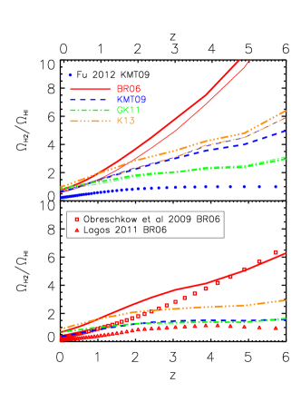
The only quantity we find to differ significantly between models based on different star formation laws is the cosmic molecular-to-atomic hydrogen ratio. The redshift evolution of this quantity is shown in Fig. 14, for all models used in this study. In the top panel, we only consider galaxies with stellar mass larger than . Thick lines are based on the MSII, while thin lines correspond to the MS. All models predict a monotonically increasing ratio with increasing redshift. Predictions from the different models are very close up to , and diverge significantly at higher redshift. In particular, the BR06 model predicts the steeper evolution, with an increase of about a factor between and . Among the models considered in our study, the milder evolution is predicted by the GK11 model. In this case, the molecular-to-atomic ratio increases by only a factor from to . The other two models, KMT09 and K13, predict similar evolution. The convergence between the two simulations is good although slightly higher values are found when using the MSII instead of the MS for the BR06 and K13 model. This is expected as the resolution limit in this case is higher than the mass threshold adopted (see Section 3.4). The blue dots shows prediction by Fu et al. (2012) based on prescriptions similar to those of our KMT09 model and on the MS. Their model predictions differ from ours both in normalization and in evolution as a function of redshift
In the bottom panel of Fig. 14, we show predictions based on the MSII only and on a lower mass threshold (), and compare them with predictions from previous work. Since the molecular-to-atomic ratio decreases for lower mass galaxies, the overall cosmic value also decreases. The trends described above remain the same: the BR06 model predicts the strongest evolution and the highest value at among all models used in our study. The weakest evolution and the lowest values are instead predicted by the GK11 and KMT09 models. This is due to the overall decrease of the stellar metallicity at higher redshift, which turns in lower values of the molecular-to-atomic ratio. The K13 model is in between the BR06 and the other two models. The red squares and triangles shown in the bottom panel of Fig. 14 correspond to predictions from Obreschkow & Rawlings (2009a) and Lagos et al. (2011a), respectively. Both assume prescriptions similar to those adopted in our BR06 model to partition the cold gas in its atomic and molecular component. The former study, however, is based on a post-processing of the model published in De Lucia & Blaizot (2007) run on the MS, while the latter is applied on Monte-Carlo merger trees. Obreschkow & Rawlings (2009a) consider all halos more massive than , while Lagos et al. (2011a) use a lower halo mass limit of . We have verified that our model predictions do not differ significantly when using instead of .
Fig. 14 shows that the cosmic evolution of is the only quantity for which predictions from different star formation laws are significantly different (although models start to differentiate only at higher redshift where important systematics in the data start playing an important role). However, the figure shows that large variations can be obtained adopting the same star formation law but different prescriptions for other physical processes, i.e. in independently developed models. This again makes it difficult to use these particular observations to put direct and strong constraints on the star formation law.
7 Summary and conclusions
We present an update of our recently published model for GAlaxy Evolution and Assembly (Hirschmann, De Lucia & Fontanot, 2016, GAEA), aimed at including a self-consistent treatment of the partition of cold gas in its atomic and molecular components. Our approach is similar to that followed in previous work based on independently developed models (Fu et al., 2010; Lagos et al., 2011b; Somerville, Popping & Trager, 2015), but our model provides significant improvements over those previously used for similar studies. In particular, GAEA: (i) includes a sophisticated chemical enrichment treatment that accounts for the non-instantaneous recycling of gas, metals, and energy; (ii) reproduces the measured relation between the metallicity of the cold gas and the galaxy stellar mass, as well as its evolution as a function of cosmic time; (iii) includes an updated modelling for stellar feedback, based partly on results from hydrodynamical simulations, and that allows us to reproduce the observed evolution of the galaxy stellar mass function.
These represent important prerequisites for our study, particularly when considering prescriptions to compute molecular-to-atomic fraction including an explicit dependence on the gas metallicity (Krumholz, McKee & Tumlinson, 2009b; Gnedin & Kravtsov, 2011; Krumholz, 2013). We also consider the empirical relation by Blitz & Rosolowsky (2006), based on the hydrostatic pressure of the disk. We find that modifying the star formation law does not translate in appreciable differences for the physical properties of galaxies or their statistical distributions. In particular, neither the number densities nor the physical properties of low-mass galaxies are significantly affected by the adoption of a molecular formation efficiency that depends on the cold gas metallicity, in contrast with previous claims (e.g. Krumholz & Dekel, 2012). As discussed in previous studies (e.g. Lagos et al., 2011b; Somerville, Popping & Trager, 2015), this behaviour arises from a self-regulation of the star formation: if less stars form (because e.g. of low molecular fractions due to low metallicities), less gas is reheated/ejected due to stellar feedback. As a result, more gas is available for star formation at later times.
All star formation laws we consider are tuned (modifying only the free parameters entering these prescriptions) in order to reproduce the local HI and H2 galaxy mass functions. For all models, we find a remarkable agreement between model predictions and the observed scaling relations between HI and H2 masses and galaxy stellar mass, distributions in optical and star forming sizes, and the relation between the cold gas phase metallicity and the galaxy stellar mass. The only quantity that exhibits significant variations depending on the different H2-based star formation laws is the cosmic molecular-to-atomic hydrogen ratio. Unfortunately, we find that similar deviations are obtained when implementing the same H2-based star formation law into independent semi-analytic models. These results suggest that it is very difficult to use available data on the gas content of galaxies to discriminate between different models. The difficulties will remain also with larger statistical samples as the scatter in most of the scaling relations is significant. A more promising avenue to put constraints on the physical processes affecting star formation laws is that of focusing on smaller galaxies and/or on galaxies at earlier cosmic epochs, as these are the regimes where self-regulation of star formation has not yet effectively washed out differences by imprinted by different star formation laws (see also Somerville, Popping & Trager, 2015).
Acknowledgements
LX and GDL acknowledge financial support from the MERAC foundation. MH acknowledges financial support from the European Research Council via an Advanced Grant under grant agreement no. 321323 NEOGAL.
References
- Baldry et al. (2012) Baldry I. K. et al., 2012, MNRAS, 421, 621
- Bennett et al. (2013) Bennett C. L. et al., 2013, ApJS, 208, 20
- Berta et al. (2013) Berta S. et al., 2013, A&A, 555, L8
- Bigiel et al. (2010) Bigiel F., Leroy A., Walter F., Blitz L., Brinks E., de Blok W. J. G., Madore B., 2010, AJ, 140, 1194
- Bigiel et al. (2008) Bigiel F., Leroy A., Walter F., Brinks E., de Blok W. J. G., Madore B., Thornley M. D., 2008, AJ, 136, 2846
- Blitz & Rosolowsky (2006) Blitz L., Rosolowsky E., 2006, ApJ, 650, 933
- Bogdán & Goulding (2015) Bogdán Á., Goulding A. D., 2015, ApJ, 800, 124
- Bolatto et al. (2008) Bolatto A. D., Leroy A. K., Rosolowsky E., Walter F., Blitz L., 2008, ApJ, 686, 948
- Booth et al. (2009) Booth R. S., de Blok W. J. G., Jonas J. L., Fanaroff B., 2009, ArXiv 0910.2935
- Boselli et al. (2014) Boselli A., Cortese L., Boquien M., Boissier S., Catinella B., Lagos C., Saintonge A., 2014, A&A, 564, A66
- Bothwell et al. (2013) Bothwell M. S. et al., 2013, MNRAS, 429, 3047
- Boylan-Kolchin et al. (2009) Boylan-Kolchin M., Springel V., White S. D. M., Jenkins A., Lemson G., 2009, MNRAS, 398, 1150
- Brown et al. (2015) Brown T., Catinella B., Cortese L., Kilborn V., Haynes M. P., Giovanelli R., 2015, MNRAS, 452, 2479
- Bruzual & Charlot (2003) Bruzual G., Charlot S., 2003, MNRAS, 344, 1000
- Calzetti et al. (2007) Calzetti D. et al., 2007, ApJ, 666, 870
- Carilli & Rawlings (2004) Carilli C. L., Rawlings S., 2004, New A Rev., 48, 979
- Catinella et al. (2013) Catinella B. et al., 2013, MNRAS, 436, 34
- Crighton et al. (2015) Crighton N. H. M. et al., 2015, MNRAS, 452, 217
- Croton et al. (2006) Croton D. J. et al., 2006, MNRAS, 365, 11
- Danovich et al. (2015) Danovich M., Dekel A., Hahn O., Ceverino D., Primack J., 2015, MNRAS, 449, 2087
- Davidzon et al. (2013) Davidzon I. et al., 2013, A&A, 558, A23
- Davis et al. (2007) Davis M. et al., 2007, ApJ, 660, L1
- De Lucia & Blaizot (2007) De Lucia G., Blaizot J., 2007, MNRAS, 375, 2
- De Lucia & Helmi (2008) De Lucia G., Helmi A., 2008, MNRAS, 391, 14
- De Lucia et al. (2014) De Lucia G., Tornatore L., Frenk C. S., Helmi A., Navarro J. F., White S. D. M., 2014, MNRAS, 445, 970
- Decarli et al. (2016) Decarli R. et al., 2016, ApJ, 833, 69
- Di Matteo et al. (2003) Di Matteo T., Croft R. A. C., Springel V., Hernquist L., 2003, ApJ, 593, 56
- Drory et al. (2004) Drory N., Bender R., Feulner G., Hopp U., Maraston C., Snigula J., Hill G. J., 2004, ApJ, 608, 742
- Dutton et al. (2011) Dutton A. A. et al., 2011, MNRAS, 410, 1660
- Elbaz et al. (2007) Elbaz D. et al., 2007, A&A, 468, 33
- Elmegreen (1989) Elmegreen B. G., 1989, ApJ, 338, 178
- Erb et al. (2006) Erb D. K., Steidel C. C., Shapley A. E., Pettini M., Reddy N. A., Adelberger K. L., 2006, ApJ, 647, 128
- Fontana et al. (2006) Fontana A. et al., 2006, A&A, 459, 745
- Förster Schreiber et al. (2009) Förster Schreiber N. M. et al., 2009, ApJ, 706, 1364
- Fu et al. (2010) Fu J., Guo Q., Kauffmann G., Krumholz M. R., 2010, MNRAS, 409, 515
- Fu et al. (2012) Fu J., Kauffmann G., Li C., Guo Q., 2012, MNRAS, 424, 2701
- Genzel et al. (2010) Genzel R. et al., 2010, MNRAS, 407, 2091
- Gil de Paz et al. (2007) Gil de Paz A. et al., 2007, ApJS, 173, 185
- Glover & Clark (2012) Glover S. C. O., Clark P. C., 2012, MNRAS, 421, 9
- Gnedin & Kravtsov (2011) Gnedin N. Y., Kravtsov A. V., 2011, ApJ, 728, 88
- Gonzalez-Perez et al. (2014) Gonzalez-Perez V., Lacey C. G., Baugh C. M., Lagos C. D. P., Helly J., Campbell D. J. R., Mitchell P. D., 2014, MNRAS, 439, 264
- Guimarães et al. (2009) Guimarães R., Petitjean P., de Carvalho R. R., Djorgovski S. G., Noterdaeme P., Castro S., Poppe P. C. D. R., Aghaee A., 2009, A&A, 508, 133
- Guo et al. (2016) Guo Q. et al., 2016, MNRAS, 461, 3457
- Guo et al. (2013) Guo Q., White S., Angulo R. E., Henriques B., Lemson G., Boylan-Kolchin M., Thomas P., Short C., 2013, MNRAS, 428, 1351
- Guo et al. (2011) Guo Q. et al., 2011, MNRAS, 413, 101
- Haas et al. (2013) Haas M. R., Schaye J., Booth C. M., Dalla Vecchia C., Springel V., Theuns T., Wiersma R. P. C., 2013, MNRAS, 435, 2955
- Haynes et al. (2011) Haynes M. P. et al., 2011, AJ, 142, 170
- Helfer et al. (2003) Helfer T. T., Thornley M. D., Regan M. W., Wong T., Sheth K., Vogel S. N., Blitz L., Bock D. C.-J., 2003, ApJS, 145, 259
- Henriques et al. (2015) Henriques B. M. B., White S. D. M., Thomas P. A., Angulo R., Guo Q., Lemson G., Springel V., Overzier R., 2015, MNRAS, 451, 2663
- Henriques et al. (2013) Henriques B. M. B., White S. D. M., Thomas P. A., Angulo R. E., Guo Q., Lemson G., Springel V., 2013, MNRAS, 431, 3373
- Hirschmann, De Lucia & Fontanot (2016) Hirschmann M., De Lucia G., Fontanot F., 2016, MNRAS, 461, 1760
- Hirschmann et al. (2012) Hirschmann M., Somerville R. S., Naab T., Burkert A., 2012, MNRAS, 426, 237
- Hopkins et al. (2014) Hopkins P. F., Kereš D., Oñorbe J., Faucher-Giguère C.-A., Quataert E., Murray N., Bullock J. S., 2014, MNRAS, 445, 581
- Hu et al. (2016) Hu C.-Y., Naab T., Walch S., Glover S. C. O., Clark P. C., 2016, MNRAS, 458, 3528
- Jaffe (1983) Jaffe W., 1983, MNRAS, 202, 995
- Jiang et al. (2015) Jiang X.-J., Wang Z., Gu Q., Wang J., Zhang Z.-Y., 2015, ApJ, 799, 92
- Johnston et al. (2015) Johnston R., Vaccari M., Jarvis M., Smith M., Giovannoli E., Häußler B., Prescott M., 2015, MNRAS, 453, 2540
- Johnston et al. (2008) Johnston S. et al., 2008, Experimental Astronomy, 22, 151
- Kauffmann & Haehnelt (2000) Kauffmann G., Haehnelt M., 2000, MNRAS, 311, 576
- Kennicutt (1989) Kennicutt, Jr. R. C., 1989, ApJ, 344, 685
- Kennicutt (1998) Kennicutt, Jr. R. C., 1998, ApJ, 498, 541
- Kennicutt et al. (2007) Kennicutt, Jr. R. C. et al., 2007, ApJ, 671, 333
- Keres, Yun & Young (2003) Keres D., Yun M. S., Young J. S., 2003, ApJ, 582, 659
- Kregel, van der Kruit & de Grijs (2002) Kregel M., van der Kruit P. C., de Grijs R., 2002, MNRAS, 334, 646
- Kroupa (2001) Kroupa P., 2001, MNRAS, 322, 231
- Krumholz (2013) Krumholz M. R., 2013, MNRAS, 436, 2747
- Krumholz & Dekel (2012) Krumholz M. R., Dekel A., 2012, ApJ, 753, 16
- Krumholz, McKee & Tumlinson (2008) Krumholz M. R., McKee C. F., Tumlinson J., 2008, ApJ, 689, 865
- Krumholz, McKee & Tumlinson (2009a) Krumholz M. R., McKee C. F., Tumlinson J., 2009a, ApJ, 693, 216
- Krumholz, McKee & Tumlinson (2009b) Krumholz M. R., McKee C. F., Tumlinson J., 2009b, ApJ, 699, 850
- Kuhlen et al. (2012) Kuhlen M., Krumholz M. R., Madau P., Smith B. D., Wise J., 2012, ApJ, 749, 36
- Lagos et al. (2011a) Lagos C. D. P., Baugh C. M., Lacey C. G., Benson A. J., Kim H.-S., Power C., 2011a, MNRAS, 418, 1649
- Lagos et al. (2012) Lagos C. d. P., Bayet E., Baugh C. M., Lacey C. G., Bell T. A., Fanidakis N., Geach J. E., 2012, MNRAS, 426, 2142
- Lagos et al. (2011b) Lagos C. D. P., Lacey C. G., Baugh C. M., Bower R. G., Benson A. J., 2011b, MNRAS, 416, 1566
- Lange et al. (2015) Lange R. et al., 2015, MNRAS, 447, 2603
- Lange et al. (2016) Lange R. et al., 2016, MNRAS, 462, 1470
- Lee et al. (2011) Lee K.-S. et al., 2011, ApJ, 733, 99
- Lee et al. (2012) Lee K.-S. et al., 2012, ApJ, 752, 66
- Leroy et al. (2009) Leroy A. K. et al., 2009, AJ, 137, 4670
- Leroy et al. (2008) Leroy A. K., Walter F., Brinks E., Bigiel F., de Blok W. J. G., Madore B., Thornley M. D., 2008, AJ, 136, 2782
- Li & White (2009) Li C., White S. D. M., 2009, MNRAS, 398, 2177
- Li, De Lucia & Helmi (2010) Li Y.-S., De Lucia G., Helmi A., 2010, MNRAS, 401, 2036
- Magdis et al. (2010) Magdis G. E., Rigopoulou D., Huang J.-S., Fazio G. G., 2010, MNRAS, 401, 1521
- Maiolino et al. (2008) Maiolino R. et al., 2008, A&A, 488, 463
- Martin et al. (2010) Martin A. M., Papastergis E., Giovanelli R., Haynes M. P., Springob C. M., Stierwalt S., 2010, ApJ, 723, 1359
- Martin & Kennicutt (2001) Martin C. L., Kennicutt, Jr. R. C., 2001, ApJ, 555, 301
- Mitchell et al. (2014) Mitchell P. D., Lacey C. G., Cole S., Baugh C. M., 2014, MNRAS, 444, 2637
- Mo, Mao & White (1998) Mo H. J., Mao S., White S. D. M., 1998, MNRAS, 295, 319
- Mo & White (2002) Mo H. J., White S. D. M., 2002, MNRAS, 336, 112
- Moustakas et al. (2013) Moustakas J. et al., 2013, ApJ, 767, 50
- Muratov et al. (2015) Muratov A. L., Kereš D., Faucher-Giguère C.-A., Hopkins P. F., Quataert E., Murray N., 2015, MNRAS, 454, 2691
- Murray & Rahman (2010) Murray N., Rahman M., 2010, ApJ, 709, 424
- Nan et al. (2011) Nan R. et al., 2011, International Journal of Modern Physics D, 20, 989
- Noeske et al. (2007) Noeske K. G. et al., 2007, ApJ, 660, L43
- Noterdaeme et al. (2012) Noterdaeme P. et al., 2012, A&A, 547, L1
- Obreschkow & Rawlings (2009a) Obreschkow D., Rawlings S., 2009a, ApJ, 696, L129
- Obreschkow & Rawlings (2009b) Obreschkow D., Rawlings S., 2009b, MNRAS, 394, 1857
- Ostriker, McKee & Leroy (2010) Ostriker E. C., McKee C. F., Leroy A. K., 2010, ApJ, 721, 975
- Pérez-González et al. (2008) Pérez-González P. G. et al., 2008, ApJ, 675, 234
- Péroux et al. (2005) Péroux C., Dessauges-Zavadsky M., D’Odorico S., Sun Kim T., McMahon R. G., 2005, MNRAS, 363, 479
- Planck Collaboration et al. (2015) Planck Collaboration et al., 2015, ArXiv 1502.01589
- Popping et al. (2015) Popping G. et al., 2015, MNRAS, 454, 2258
- Popping, Somerville & Trager (2014) Popping G., Somerville R. S., Trager S. C., 2014, MNRAS, 442, 2398
- Prochaska & Wolfe (2009) Prochaska J. X., Wolfe A. M., 2009, ApJ, 696, 1543
- Rao, Turnshek & Nestor (2006) Rao S. M., Turnshek D. A., Nestor D. B., 2006, ApJ, 636, 610
- Robitaille & Whitney (2010) Robitaille T. P., Whitney B. A., 2010, ApJ, 710, L11
- Sabra et al. (2015) Sabra B. M., Saliba C., Abi Akl M., Chahine G., 2015, ApJ, 803, 5
- Saintonge et al. (2011) Saintonge A. et al., 2011, MNRAS, 415, 32
- Saintonge et al. (2013) Saintonge A. et al., 2013, ApJ, 778, 2
- Salim et al. (2007) Salim S. et al., 2007, ApJS, 173, 267
- Salmi et al. (2012) Salmi F., Daddi E., Elbaz D., Sargent M. T., Dickinson M., Renzini A., Bethermin M., Le Borgne D., 2012, ApJ, 754, L14
- Sanders et al. (2015) Sanders R. L. et al., 2015, ApJ, 799, 138
- Santini et al. (2009) Santini P. et al., 2009, A&A, 504, 751
- Schaye et al. (2010) Schaye J. et al., 2010, MNRAS, 402, 1536
- Schechter (1976) Schechter P., 1976, ApJ, 203, 297
- Schmidt (1959) Schmidt M., 1959, ApJ, 129, 243
- Shen et al. (2003) Shen S., Mo H. J., White S. D. M., Blanton M. R., Kauffmann G., Voges W., Brinkmann J., Csabai I., 2003, MNRAS, 343, 978
- Sobral et al. (2014) Sobral D., Best P. N., Smail I., Mobasher B., Stott J., Nisbet D., 2014, MNRAS, 437, 3516
- Somerville, Popping & Trager (2015) Somerville R. S., Popping G., Trager S. C., 2015, MNRAS, 453, 4337
- Speagle et al. (2014) Speagle J. S., Steinhardt C. L., Capak P. L., Silverman J. D., 2014, ApJS, 214, 15
- Springel et al. (2005) Springel V. et al., 2005, Nature, 435, 629
- Steidel et al. (2014) Steidel C. C. et al., 2014, ApJ, 795, 165
- Stevens et al. (2017) Stevens A. R. H., del P. Lagos C., Contreras S., Croton D. J., Padilla N. D., Schaller M., Schaye J., Theuns T., 2017, MNRAS
- Tacconi et al. (2013) Tacconi L. J. et al., 2013, ApJ, 768, 74
- Toomre (1964) Toomre A., 1964, ApJ, 139, 1217
- Tremonti et al. (2004) Tremonti C. A. et al., 2004, ApJ, 613, 898
- van der Wel et al. (2014) van der Wel A. et al., 2014, ApJ, 788, 28
- Volonteri, Natarajan & Gültekin (2011) Volonteri M., Natarajan P., Gültekin K., 2011, ApJ, 737, 50
- Walter et al. (2008) Walter F., Brinks E., de Blok W. J. G., Bigiel F., Kennicutt, Jr. R. C., Thornley M. D., Leroy A., 2008, AJ, 136, 2563
- Walter et al. (2014) Walter F. et al., 2014, ApJ, 782, 79
- Wang et al. (2008) Wang J., De Lucia G., Kitzbichler M. G., White S. D. M., 2008, MNRAS, 384, 1301
- Weinmann et al. (2012) Weinmann S. M., Pasquali A., Oppenheimer B. D., Finlator K., Mendel J. T., Crain R. A., Macciò A. V., 2012, MNRAS, 426, 2797
- White, Somerville & Ferguson (2015) White C. E., Somerville R. S., Ferguson H. C., 2015, ApJ, 799, 201
- Wolfire et al. (2003) Wolfire M. G., McKee C. F., Hollenbach D., Tielens A. G. G. M., 2003, ApJ, 587, 278
- Wong & Blitz (2002) Wong T., Blitz L., 2002, ApJ, 569, 157
- Wootten & Thompson (2009) Wootten A., Thompson A. R., 2009, IEEE Proceedings, 97, 1463
- Zafar et al. (2013) Zafar T., Péroux C., Popping A., Milliard B., Deharveng J.-M., Frank S., 2013, A&A, 556, A141
- Zhao et al. (2009) Zhao D. H., Jing Y. P., Mo H. J., Börner G., 2009, ApJ, 707, 354
- Zoldan et al. (2017) Zoldan A., De Lucia G., Xie L., Fontanot F., Hirschmann M., 2017, MNRAS, 465, 2236
- Zwaan et al. (2005) Zwaan M. A., Meyer M. J., Staveley-Smith L., Webster R. L., 2005, MNRAS, 359, L30
Appendix A Comparison between different models for disk sizes
In Section 2.2, we introduce our updated model for disk sizes, based on accumulation of angular momentum through different physical processes. In this section, we compare model predictions obtained using the semi-analytic model described in HDLF16 with its original prescriptions to model disk sizes, and our updated modelling.

The left and middle panels of Fig. 15 show the half-mass radius of the gaseous and stellar disks as a function of galaxy stellar mass. Using our updated model for disk size, both radii are larger than using the disk model adopted in HDLF16, particularly for stellar masses larger than log. The most massive galaxies are bulge dominated and acquired their stellar mass primarily through mergers and accretions of lower mass systems. In the original model used in HDLF16, the size of the disk was not updated during galaxy mergers, while we now trace sizes of both components adopting a physically motivated scheme. If we consider only disk-dominated (), star forming galaxies with specific star formation rate sSFR, the two models predict a very similar size-mass relation. Results are shown in the right panel of Fig. 15 where we consider the half-mass radius of the composed system disk+bulge.
It is worth stressing that, although there are significant differences between the disk sizes of massive galaxies predicted by the HDLF16 model and by the same physical model adopting our updated prescriptions for disk size, this does not introduce significant differences for other galaxy properties or statistics such as e.g. the galaxy stellar mass function and other scaling relations.
Appendix B Resolution tests
We use the MS and MSII to quantify the resolution limits in our model. These two simulations are based on the same cosmological model and are run using the same simulation code, but the mass resolution of MSII is 125 times higher than that of the MS.
Fig. 16 shows the galaxy stellar mass function predicted by the model presented in Hirschmann, De Lucia & Fontanot (2016, their FIRE feedback scheme), both based on the MS (dashed black line) and the MSII (dashed red line). The figure shows that the convergence is good over the mass range log, while the model based on the MS tends to under-predict the number densities of most massive galaxies with respect to the model based on the MSII. Fig. 17 shows the corresponding results for the cold gas mass function. Also in this case, there is a discrepancy at the massive end, with the MS corresponding to lower number densities of gas rich galaxies with respect to the MSII.
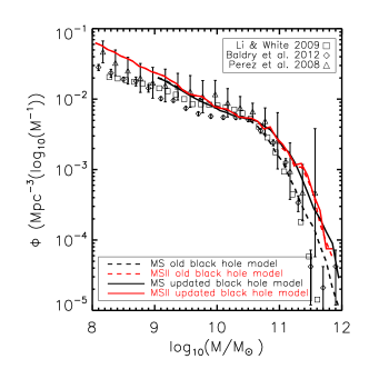
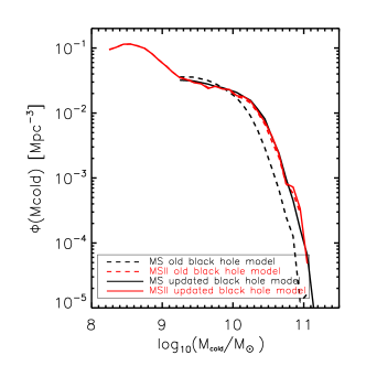
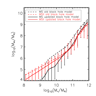
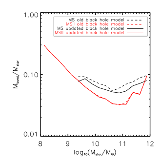
We find that this is largely due to a difference in the black hole masses: specifically, if we switch off the accretion onto black holes during galaxy mergers, predictions based on the MS and MSII for the galaxy stellar mass function are consistent at the massive end. Fig. 18 shows the relation between the black hole mass and the galaxy stellar mass. When considering the HDLF16 model, the relation based on the MSII is shifted down with respect to that based on the MS by about dex. The more massive black holes in the MS cause a more efficient suppression of galaxy formation (via AGN feedback) at the massive end. Thus, the galaxy stellar mass function based on the MS is below that based on the MSII.
The results described above can be understood as follows: at early redshift, star formation driven by cooling flows dominates the evolution of galaxies. In the MSII, dark matter halos are resolved earlier than that in the MS, and so star formation starts earlier, locking a fraction of the gas available in stars. Therefore, when the first mergers take place, less gas is available to fuel the black hole growth. In the MS, the first resolved haloes are identified at later times with respect to the MSII. As these haloes are in the rapid cooling regime, larger amount of cold gas are dumped into the galaxies and become available for black hole growth during the first galaxy mergers. In our model, gas rich mergers also result in a larger fraction of stars formed during mergers. To quantify the importance of this channel, we record the mass of stars formed in mergers for runs based on both simulations. Fig. 19 shows the median fraction of with respect to the galaxy stellar mass as a function of the latter. For the MS, the fraction is about times larger than that obtained for the MSII. In both simulations, however, bursts contribute for less than per cent of the total stellar mass for galaxies with . Thus we argue that the main reason for the differences seen in the galaxy stellar mass function and cold gas mass function is due to the systematic differences in the black hole growth.
As explained in Section 2.3, we update the black hole model used in HDLF16 by ‘planting a black hole seed’ in each galaxy sitting at the centre of a halo with virial temperatures above K. We rerun our resolution tests using the same physical model adopted in HDLF16 but including our updated black hole model. The solid lines shown in Figs. 16, 17, and 18 show results from these tests. Both the galaxy stellar mass function and the cold gas mass function now converge well at the most massive end. Our updated black hole growth model also predicts consistent results for the relation between the black hole mass and the galaxy stellar mass (see solid lines in Fig. 18), although black holes tend to be more massive in the MSII for galaxies with .
Appendix C Different choices of and
This section presents results of different tests related to the definition of the interstellar radiation field () within the GK11 model, and of the density of dark matter and stars () within the K13 model.
Our default assumption for is given by the star formation rate integrated over the entire gaseous disk, averaged over the time interval between two subsequent snapshots and normalized to the current rate of star formation estimated for our Galaxy. As discussed in Section 2.4.3, however, it would be more physical to express the interstellar radiation field in terms of the surface density of star formation rate. In Fig. 20, we compare the predicted galaxy stellar mass function (left panel), HI mass function (middle panel) and H2 mass function (right panel) from our GK11 model with results obtained using two alternative prescriptions for . In particular, blue lines correspond to a model where is assumed to be proportional to the surface density of star formation averaged over the entire disk. In this case, we assume the normalization factor to be . Red lines correspond to a model using the same assumption but within each disk annulus. The figure shows that differences between these different assumptions are very small (less than dex at the low mass end in all three panels).
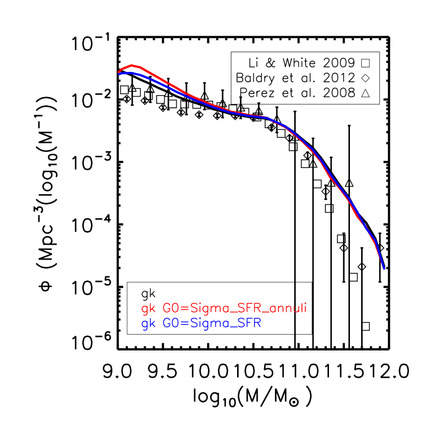
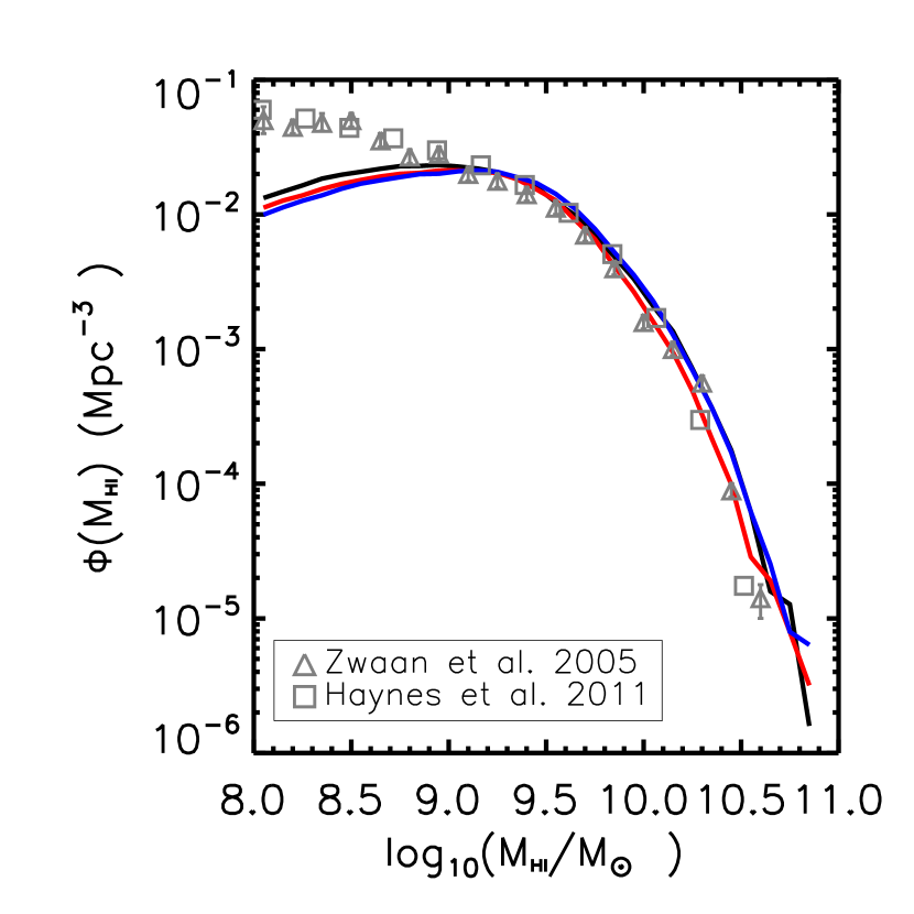
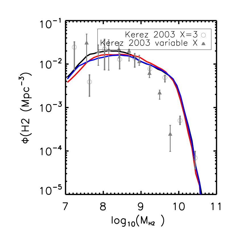
Fig. 21 shows a similar comparison but this time for tests made using different assumptions to compute within the K13 model. As explained in Section 2.4.3, our default model uses the calculator provided by Zhao et al. (2009) to assign a concentration to any halo in the simulation. Assuming a NFW profile, this allows us to compute the density of dark matter. Red lines shown in Fig. 21 correspond to a model adopting the lower limit given by the fitting formula provided by Krumholz (2013). We find that this parameter has little influence on the final model results and so significant amounts of computational time can be saved using a simpler approximation.