Correlation functions in theories
with Lifshitz scaling

Abstract

The 2+1 dimensional quantum Lifshitz model can be generalised to a class of higher dimensional free field theories that exhibit Lifshitz scaling. When the dynamical critical exponent equals the number of spatial dimensions, equal time correlation functions of scaling operators in the generalised quantum Lifshitz model are given by a d-dimensional higher-derivative conformal field theory. Autocorrelation functions in the generalised quantum Lifshitz model in any number of dimensions can on the other hand be expressed in terms of autocorrelation functions of a two-dimensional conformal field theory. This also holds for autocorrelation functions in a strongly coupled Lifshitz field theory with a holographic dual of Einstein-Maxwell-dilaton type. The map to a two-dimensional conformal field theory extends to autocorrelation functions in thermal states and out-of-equilbrium states preserving symmetry under spatial translations and rotations in both types of Lifshitz models. Furthermore, the spectrum of quasinormal modes of scalar field perturbations in Lifshitz black hole backgrounds can be obtained analytically at low spatial momenta and exhibits a linear dispersion relation at z = d. At high momentum, the mode spectrum can be obtained in a WKB approximation and displays very different behaviour compared to holographic duals of conformal field theories. This has implications for thermalisation in strongly coupled Lifshitz field theories with $z>1$.

1 Introduction

A second order quantum phase transition is characterized by a dynamical critical scaling exponent $z$, which dictates the form of the scaling symmetry present at the zero temperature critical point,

$$\vec{x}\rightarrow\lambda\vec{x},\quad\tau\rightarrow\lambda^{z}\tau\,,$$ (1)

where $\vec{x}=(x^{1},\ldots,x^{d})$ are spatial coordinates and $\tau$ is Euclidean time. In relativistic systems $z=1$ and the scaling symmetry is extended to the full conformal symmetry. Generic quantum critical points in non-relativistic systems, on the other hand, do not have conformal symmetry and exhibit anisotropic scaling between time and the spatial directions with $z>1$, commonly referred to as Lifshitz scaling. In this paper we study correlation functions of scaling operators in theories with Lifshitz scaling in $d\geq 2$ spatial dimensions. We pay particular attention to so-called autocorrelators, i.e. correlation functions where all the operators are inserted at the same spatial point but at different times,

$$\langle\mathcal{O}_{1}(\vec{x},t_{1})\mathcal{O}_{2}(\vec{x},t_{2})...\mathcal{O}_{n}(\vec{x},t_{n})\rangle\,.$$ (2)

Autocorrelators carry information about the energy spectrum of the model in question and provide a useful diagnostic of time evolution in out of equilibrium configurations.

We begin in Section 2 by introducing a set of free field theories in $d{+}1$ dimensions that realise Lifshitz scaling with arbitrary dynamical critical exponent. These theories include the well known $2{+}1$-dimensional quantum Lifshitz model as a special case with $z=d=2$ and provide a particularly simple setting to study quantum critical behaviour at generic integer values of $z$. Many interesting properties of the original quantum Lifshitz model survive in the more general free field theories when the dynamical critical exponent $z$ equals the number of spatial dimensions and we refer to the models with $z=d$ as generalised quantum Lifshitz models. For instance, it is well known that the ground state correlation functions of scaling operators at equal time in the original quantum Lifshitz model can be expressed in terms of correlation functions of a two-dimensional Euclidean field theory with conformal symmetry Ardonne:2003wa . We briefly review this construction and then show how the connection to conformal field theory extends to $d{+}1$-dimensions, provided that $z=d$, in which case the connection is to a higher-derivative free field CFT in $d$ dimensions.

There is a further connection to conformal field theory, which is only realised in the time domain. It turns out that autocorrelators in the generalised quantum Lifshitz model in any number of dimensions can be expressed in terms of autocorrelators of a two-dimensional conformal field theory when $z=d$. This holds for autocorrelators evaluated in any Gaussian state that is symmetric under spatial translations and rotations, and as a non-trivial example we work out autocorrelators of monopole operators in a thermal state.

Since the generalised quantum Lifshitz model is a free field theory, it is perhaps not that surprising that its correlation functions take a simple form. It turns out, however, that the connection to two-dimensional conformal field theory persists when one considers autocorrelators in a strongly coupled field theory with a holographic dual that exhibits Lifshitz scaling. In Section 3 we introduce a holographic model that realises Lifshitz scaling with generic $z>1$ and evaluate vacuum two-point functions of operators with large scaling dimension. Analytic expressions are easily obtained for the equal time two-point function and the two-point autocorrelator at general $d$ and $z$. For the special case of $z=2$ we find a parametrized solution for the full vacuum two-point function at arbitrary spatial and temporal separation on the boundary and compare it to the corresponding correlation function in the quantum Lifshitz model. We then turn our attention to more general autocorrelators in the holographic model and uncover a quantitative relation to autocorrelators in a two-dimensional conformal field theory. In particular, we show how the form of three-point autocorrelators at general $d$ and $z$ is constrained by an underlying two-dimensional extended symmetry.

In Section 4 we restrict to integer values of $z=d$ and show how autocorrelators in a thermal state in the holographic model can be expressed in terms of thermal autocorrelators of a two-dimensional conformal field theory. The resulting thermal two- and three-point autocorrelators in the holographic theory thus have the same scaling form as those of the generalised quantum Lifshitz model.

In Section 5 we venture outside the time domain and consider quasinormal modes of massive scalar field fluctuations at finite momentum. In momentum space we can go beyond the geodesic approximation and find that the special behaviour at $z=d$ persists at small momentum and any operator scaling dimension. In Appendix C we expand on the numerical and analytic methods we use to study the quasinormal mode spectrum and extend our discussion to include quasinormal modes at any $z$, $d$ and high momentum.

The connection between generalised Lifshitz models at $z=d$ and two-dimensional conformal field theory extends to more general states that are invariant under spatial translations and rotations. This includes time-dependent states dual to Lifshitz-Vaidya spacetimes in the holographic models and quench states in the generalised quantum Lifshitz model, as briefly illustrated in Section 6.

We conclude our discussion in Section 7 and some technical results that are referred to in the main text are worked out in the appendices.

2 The generalised quantum Lifshitz model

Our starting point is a class of $d{+}1$-dimensional quantum field theories exhibiting Lifshitz scaling with integer valued dynamical critical exponent $z$. They are governed by the following (Euclidean) action

$$S=\frac{1}{2}\int d^{d}xd\tau\Big{[}(\partial_{\tau}\chi)^{2}+\kappa^{2}(\nabla^{z}\chi)^{2}\Big{]},$$ (3)

where $\kappa>0$ is a constant and we are using a shorthand notation,

$$\nabla^{z}\chi=\left\{\begin{array}[]{cll}(\nabla^{2})^{k}\chi&\textrm{if}&z=2k\,,\\ (\nabla^{2})^{k}\vec{\nabla}\chi&\textrm{if}&z=2k{+}1\,.\end{array}\right.$$ (4)

These models generalise the well known quantum Lifshitz model Ardonne:2003wa , which has $z=2$ in $2{+}1$ dimensions, and allow us to systematically explore the behaviour of various physical quantities at different values of the dynamical critical exponent in a controlled free field theory setting. When there are explicit analytic results available one can even consider formally extending $z$ to non-integer values. In the following we will mainly be concerned with theories where $z=d$, which includes the quantum Lifshitz model as a special case. The connection to conformal field theory found in the quantum Lifshitz model is retained at general $z=d>2$ and accordingly we refer to these theories as generalised quantum Lifshitz models.

The generalised monopole operators (or just monopole operators for short),

$$\mathcal{O}_{\alpha}(\vec{x},t)=e^{i\alpha\chi(\vec{x},t)},$$ (5)

with $\alpha\in\mathbf{R}$, turn out to have simple scaling properties in the generalised quantum Lifshitz model and we will focus our attention on their correlation functions. The name monopole operator arises from a dual gauge field representation of the original quantum Lifshitz model, where such operators with $\alpha=\pm 2\pi$ create magnetic monopoles in three-dimensional Euclidean space Ardonne:2003wa .

2.1 Equal time correlation functions

The ground state wave functional of the quantum Lifshitz model with $z=d=2$ is given by the exponential of a Euclidean action of a free $1{+}1$-dimensional conformal field theory (CFT) Ardonne:2003wa . In Appendix A we outline how this statement can be generalised to arbitrary $z=d$ by expressing the ground state wave functional in terms of a free $d$-dimensional (higher-derivative) CFT of a type studied recently in Brust:2016gjy . The connection to a CFT can also be obtained by showing that equal time correlation functions of monopole operators in the generalised quantum Lifshitz model have the form of CFT correlation functions,

$$\langle\mathcal{O}_{\alpha_{1}}(\vec{x}_{1},\tau)\ldots\mathcal{O}_{\alpha_{n}}(\vec{x}_{n},\tau)\rangle=\big{\langle}e^{i\alpha_{1}\chi(\vec{x}_{1})}\ldots e^{i\alpha_{n}\chi(\vec{x}_{n})}\big{\rangle}_{CFT}.$$ (6)

Consider the vacuum two-point function of the $\chi$ field,

$$G_{E}(\vec{x}_{1},\tau_{1};\vec{x}_{2},\tau_{2})=\int\frac{d\omega d^{d}p}{(2\pi)^{d+1}}\frac{e^{-i\omega(\tau_{1}-\tau_{2})-i\vec{p}\cdot(\vec{x}_{1}-\vec{x}_{2})}}{\omega^{2}+\kappa^{2}p^{2z}}\,,$$ (7)

where $p=|\vec{p}|$ and we let $z$ take a general integer value for now. The integral over $\omega$ is easily performed by closing the integration contour around the upper or lower half of the complex $\omega$-plane, depending on the sign of $\tau_{12}\equiv\tau_{1}-\tau_{2}$. Either way, a single residue at $\omega=\pm i\kappa p^{z}$ is picked out, giving

$$G_{E}(\vec{x}_{1},\tau_{1};\vec{x}_{2},\tau_{2})=\frac{1}{2\kappa}\int\frac{d^{d}p}{(2\pi)^{d}}\frac{1}{p^{z}}e^{-\kappa|\tau_{12}|p^{z}-i\vec{p}\cdot\vec{x}_{12}},$$ (8)

where $\vec{x}_{12}\equiv\vec{x}_{1}-\vec{x}_{2}$. The remaining momentum integral is convergent for $z<d$, logarithmically divergent for $z=d$, and power-law divergent for $z>d$.

For equal time correlation functions we set $\tau_{1}=\tau_{2}$ in (8) and then the two-point function becomes formally identical to the two-point function of a free scalar field in $d$-dimensions with the action

$$S=\kappa\int d^{d}x\phi(-\nabla^{2})^{z/2}\phi\,.$$ (9)

At $z=d$ with $d$ an even integer, this is one of the higher-derivative free scalar CFTs considered in Brust:2016gjy .

Equal time correlation functions of monopole operators are obtained by applying Wick’s theorem, and the connection (6) follows from the equality of the two-point functions of the elementary fields at equal time in the generalised quantum Lifshitz model and the free $d$-dimensional CFT. So far, we have written down formal expressions which need to be supplemented by prescriptions for both IR and UV regularisation. To address such issues, and in order to establish some notation for later use, it is useful to work out some explicit examples, starting with the equal time correlation function of two monopole operators,

$$\langle\mathcal{O}_{\alpha_{1}}(\vec{x}_{1},\tau)\mathcal{O}_{\alpha_{2}}(\vec{x}_{2},\tau)\rangle = \Big{\langle}e^{i\alpha_{1}\chi(\vec{x}_{1})}e^{i\alpha_{2}\chi(\vec{x}_{2})}\Big{\rangle}$$ (10)

$$= e^{-\frac{1}{2}\alpha_{1}^{2}G_{E}(\vec{x}_{1};\vec{x}_{1})-\frac{1}{2}\alpha_{2}^{2}G_{E}(\vec{x}_{2};\vec{x}_{2})-\alpha_{1}\alpha_{2}G_{E}(\vec{x}_{1};\vec{x}_{2})}.$$

The equal time $G_{E}(\vec{x}_{1};\vec{x}_{2})$ is given by (8) with $z=d$ and $\tau_{1}=\tau_{2}$,

$$G_{E}(\vec{x}_{1};\vec{x}_{2}) = \frac{1}{2\kappa}\int\frac{d^{d}p}{(2\pi)^{d}}\frac{e^{-i\vec{p}\cdot\vec{x}_{12}}}{p^{d}}$$ (11)

$$= \frac{\text{Vol}(S^{d-2})}{2\kappa(2\pi)^{d}}\int_{0}^{\infty}dp\int_{0}^{\pi}d\theta(\sin\theta)^{d-2}\frac{e^{-ip|\vec{x}_{12}|\cos\theta}}{p+\mu}\,,$$

where the parameter $\mu>0$, introduced to regulate the infrared divergence in the integral over $p$, is to be sent to zero at the end of the calculation.

The integral over $\theta$ evaluates to a Bessel function,

$$\int_{0}^{\pi}d\theta(\sin\theta)^{d-2}e^{-ip|\vec{x}_{12}|\cos\theta}=2^{(d{-}2)/2}\sqrt{\pi}\Gamma({\textstyle\frac{d-1}{2}})\big{(}p|\vec{x}_{12}|\big{)}^{1-{\textstyle\frac{d}{2}}}J_{{\textstyle\frac{d}{2}}-1}(p|\vec{x}_{12}|),$$

and using $\text{Vol}(S^{d-2})=2\pi^{(d-1)/2}/\Gamma(\frac{d-1}{2})$ we obtain

$$G_{E}(\vec{x}_{1};\vec{x}_{2}) = \frac{1}{2\kappa(2\pi)^{d/2}}\int_{0}^{\infty}dy\,\frac{y^{1-{\textstyle\frac{d}{2}}}}{y+\mu|\vec{x}_{12}|}\,J_{{\textstyle\frac{d}{2}}-1}(y)$$ (12)

$$= -\,\frac{1}{2^{d}\pi^{d/2}\Gamma(d/2)\kappa}\big{(}\log(\mu|\vec{x}_{12}|)+c_{d}+\ldots\big{)},$$

where $c_{d}$ is a finite constant and $\ldots$ denotes terms that vanish in the limit $\mu\rightarrow 0$. Inserting this expression for $G_{E}(\vec{x}_{1};\vec{x}_{2})$ into (10) then gives

$$\big{\langle}\mathcal{O}_{\alpha_{1}}(\vec{x}_{1},\tau)\mathcal{O}_{\alpha_{2}}(\vec{x}_{2},\tau)\big{\rangle}=\big{(}\mu e^{c_{d}}\big{)}^{\frac{(\alpha_{1}+\alpha_{2})^{2}}{2^{d+1}\pi^{d/2}\Gamma(d/2)\kappa}}\,\epsilon^{\frac{\alpha^{2}_{1}+\alpha^{2}_{2}}{2^{d+1}\pi^{d/2}\Gamma(d/2)\kappa}}\,|\vec{x}_{12}|^{\frac{\alpha_{1}\alpha_{2}}{2^{d}\pi^{d/2}\Gamma(d/2)\kappa}}\,,$$ (13)

where we have introduced an ultraviolet cutoff,

$$|\vec{x}_{ij}|\geq\epsilon\,,$$ (14)

to regulate the self-contractions in Wick’s theorem. As a result, the equal time two-point function of monopole operators is independent of the infrared regulator when $\alpha_{1}+\alpha_{2}=0$ but vanishes when $\mu\rightarrow 0$ unless this condition on the charges is satisfied. The dependence on the ultraviolet cutoff can be absorbed into a renormalisation of the monopole operator when viewed as a composite operator,

$$\mathcal{O}_{\alpha}^{R}(\vec{x},\tau)\equiv\epsilon^{-\Delta}e^{i\alpha\chi(\vec{x}_{i},\tau)}\,,$$ (15)

of scaling dimension

$$\Delta=\frac{\alpha^{2}}{2^{d+1}\pi^{d/2}\Gamma\left(\frac{d}{2}\right)\kappa}\,.$$ (16)

The equal time two-point function of renormalized monopole operators then reduces to the usual scaling form,

$$\langle\mathcal{O}_{\alpha}^{R}(\vec{x}_{1},\tau)\mathcal{O}_{-\alpha}^{R}(\vec{x}_{2},\tau)\rangle=|\vec{x}_{12}|^{-2\Delta}.$$ (17)

The equal time correlation function of three monopole operators is obtained in a similar fashion,

$$\langle \mathcal{O}_{\alpha_{1}}(\vec{x}_{1},\tau)\mathcal{O}_{\alpha_{2}}(\vec{x}_{2},\tau)\mathcal{O}_{\alpha_{3}}(\vec{x}_{3},\tau)\rangle$$

$$=e^{-\frac{1}{2}\sum_{i,j=1}^{3}\alpha_{i}\alpha_{j}G_{E}(\vec{x}_{i};\vec{x}_{j})}$$ (18)

$$=\big{(}\mu e^{c_{d}}\big{)}^{\frac{(\alpha_{1}+\alpha_{2}+\alpha_{3})^{2}}{2^{d+1}\pi^{d/2}\Gamma(d/2)\kappa}}\epsilon^{\Delta_{1}+\Delta_{2}+\Delta_{3}}|\vec{x}_{12}|^{\Delta_{3}-\Delta_{1}-\Delta_{2}}|\vec{x}_{13}|^{\Delta_{2}-\Delta_{3}-\Delta_{1}}|\vec{x}_{23}|^{\Delta_{1}-\Delta_{2}-\Delta_{3}}\,.$$

This expression vanishes in the $\mu\rightarrow 0$ limit unless $\alpha_{1}+\alpha_{2}+\alpha_{3}=0$ but when the sum of charges is zero the equal time three-point function of renormalised monopole operators reduces to a standard CFT form,

$$\langle\mathcal{O}^{R}_{\alpha_{1}}(\vec{x}_{1},\tau)\mathcal{O}^{R}_{\alpha_{2}}(\vec{x}_{2},\tau)\mathcal{O}^{R}_{\alpha_{3}}(\vec{x}_{3},\tau)\rangle=|\vec{x}_{12}|^{\Delta_{3}-\Delta_{1}-\Delta_{2}}|\vec{x}_{13}|^{\Delta_{2}-\Delta_{3}-\Delta_{1}}|\vec{x}_{23}|^{\Delta_{1}-\Delta_{2}-\Delta_{3}}\,.$$ (19)

Finally, a straightforward calculation gives the equal time correlation function of four renormalised monopole operators with $\sum_{i=1}^{4}\alpha_{i}=0$ in terms of invariant cross ratios,

$$\langle\mathcal{O}^{R}_{\alpha_{1}}(\vec{x}_{1},\tau)\ldots\mathcal{O}^{R}_{\alpha_{4}}(\vec{x}_{4},\tau)\rangle =\epsilon^{-\widetilde{\Delta}}e^{-\frac{1}{2}\sum_{i,j=1}^{4}\alpha_{i}\alpha_{j}G_{E}(\vec{x}_{i};\vec{x}_{j})}$$ (20)

$$=\prod_{i<j}|\vec{x}_{ij}|^{\frac{\widetilde{\Delta}}{3}-\Delta_{i}-\Delta_{j}}X^{\frac{\widetilde{\Delta}}{3}-\frac{(\alpha_{1}+\alpha_{3})^{2}}{2^{d+1}\pi^{d/2}\Gamma(d/2)\kappa}}Y^{\frac{\widetilde{\Delta}}{3}-\frac{(\alpha_{1}+\alpha_{4})^{2}}{2^{d+1}\pi^{d/2}\Gamma(d/2)\kappa}}\,,$$

where $X=\frac{|\vec{x}_{12}|\,|\vec{x}_{34}|}{|\vec{x}_{13}|\,|\vec{x}_{24}|}$, $Y=\frac{|\vec{x}_{12}|\,|\vec{x}_{34}|}{|\vec{x}_{14}|\,|\vec{x}_{23}|}$ and $\widetilde{\Delta}=\sum_{i=1}^{4}\Delta_{i}$.

2.2 Operators inserted at generic points

We now turn our attention to correlation functions in the generalised quantum Lifshitz model with operators inserted at different times as well as different spatial positions. For this we find it convenient to adopt a streamlined regularisation procedure along the lines of the one used by Ardonne:2003wa in the original quantum Lifshitz model. Having established that non-vanishing correlation functions of monopole operators are independent of the infrared regulator, we can dispense with $\mu$ in our formulas, provided we only consider correlation functions where the monopole charges satisfy $\sum_{i}\alpha_{i}=0$. The ultraviolet divergences are then efficiently handled by introducing a regularised two-point function with the equal time coincident point two-point function subtracted off. Starting from (8) we obtain

$$G^{R}_{E}(\vec{x}_{1},\tau_{1} ;\vec{x}_{2},\tau_{2})\equiv G_{E}(\vec{x}_{1},\tau_{1};\vec{x}_{2},\tau_{2})-G_{E}(\vec{x}_{1},\tau_{1};\vec{x}_{2},\tau_{2})\Big{|}_{\{|\vec{x}_{12}|=\epsilon,\ \tau_{12}=0\}}$$

$$=\frac{1}{2\kappa(2\pi)^{d/2}}\int_{0}^{\infty}\frac{dp}{p}\left[\big{(}p|\vec{x}_{12}|\big{)}^{1-{\textstyle\frac{d}{2}}}J_{{\textstyle\frac{d}{2}}-1}(p|\vec{x}_{12}|)e^{-\kappa|\tau_{12}|p^{d}}-\big{(}p\epsilon\big{)}^{1-{\textstyle\frac{d}{2}}}J_{{\textstyle\frac{d}{2}}-1}(p\epsilon)\right]$$

$$=\frac{1}{2\kappa(2\pi)^{d/2}}\int_{0}^{\infty}dy\,y^{-d/2}\Big{[}J_{{\textstyle\frac{d}{2}}-1}(y)e^{-\xi y^{d}}-\left|\frac{\vec{x}_{12}}{\epsilon}\right|^{{\textstyle\frac{d}{2}}-1}J_{{\textstyle\frac{d}{2}}-1}\big{(}\frac{\epsilon y}{|\vec{x}_{12}|}\big{)}\Big{]},$$ (21)

where in the last step we have introduced a scaling variable,

$$\xi\equiv\frac{\kappa|\tau_{12}|}{|\vec{x}_{12}|^{d}}\,,$$ (22)

which is invariant under the Lifshitz scaling transformation (1) with $z=d$.

The equal time correlation functions of renormalised monopole operators are easily recovered by setting $\xi=0$ in the regularised two-point function. In this case the integral in (21) can be obtained in closed form and one finds the following exact result for the regularised equal time two-point function,

$$G^{R}_{E}(\vec{x}_{1};\vec{x}_{2})=-\,\frac{1}{2^{d}\pi^{d/2}\Gamma\left(\frac{d}{2}\right)\kappa}\log\Big{(}\frac{|\vec{x}_{12}|}{\epsilon}\Big{)}.$$ (23)

Wick’s theorem then yields the same equal time correlation functions of monopole operators as in Section 2.1.

The regularised two-point function at generic points can be expressed as a sum of two terms: the equal time two-point function (23) and an integral that only depends on the Lifshitz invariant combination $\xi$,

$$G^{R}_{E}(\vec{x}_{1},\tau_{1};\vec{x}_{2},\tau_{2})=G^{R}_{E}(\vec{x}_{1};\vec{x}_{2})\Big{|}_{\xi=0}+I_{d}(\xi)\,,$$ (24)

with

$$I_{d}(\xi)=\frac{1}{2\kappa(2\pi)^{d/2}}\int_{0}^{\infty}dy\,y^{-d/2}J_{{\textstyle\frac{d}{2}}-1}(y)\big{(}e^{-\xi y^{d}}-1\big{)}\,.$$ (25)

The integral is finite for any finite value of $\xi$ and can easily be evaluated numerically for any given number of spatial dimensions. Correlation functions of monopole operators inserted at generic points do not have the CFT form found for equal time correlators but depend on the Lifshitz invariant ratio $\xi$ in a non-trivial way. For instance, the correlation function of two renormalised monopole operators is given by

$$\langle\mathcal{O}_{\alpha}^{R}(\vec{x}_{1},\tau_{1})\mathcal{O}_{-\alpha}^{R}(\vec{x}_{2},\tau_{2})\rangle=|\vec{x}_{12}|^{-2\Delta}\,e^{\alpha^{2}I_{d}(\xi)}.$$ (26)

In the special case of $d=2$, the integral can be expressed in terms of an incomplete gamma function

$$I_{2}(\xi)=-\,\frac{1}{8\pi\kappa}\Gamma\big{(}0,\frac{1}{4\xi}\big{)}\,,$$ (27)

and we reproduce the monopole operator two-point function of Ardonne:2003wa for the original quantum Lifshitz model,

$$\langle\mathcal{O}_{\alpha}^{R}(\vec{x}_{1},\tau_{1})\mathcal{O}_{-\alpha}^{R}(\vec{x}_{2},\tau_{2})\rangle=|\vec{x}_{12}|^{-2\Delta}\,e^{-\Delta\Gamma\big{(}0,\frac{|\vec{x}_{12}|^{2}}{4\kappa|\tau_{12}|}\big{)}}.$$ (28)

2.3 Vacuum autocorrelators

Next we consider monopole operators located at the same spatial point but at different times and evaluate the resulting autocorrelation functions. This amounts to taking the limit $|\vec{x}_{ij}|\rightarrow 0$ for all the spatial insertion points before using Wick’s theorem to evaluate the correlation function of the monopole operators. At first sight, the regularised two-point function (24) appears singular in this limit, due to the logarithmic dependence on $|\vec{x}_{12}|$ in the equal time two-point function (23), but this turns out to be cancelled by a corresponding logarithm in the integral $I_{d}(\xi)$ at large $\xi$.

To see this, we differentiate $I_{d}$ with respect to $\xi$,

$$\frac{dI_{d}}{d\xi}=-\,\frac{1}{2(2\pi)^{d/2}\kappa}\int_{0}^{\infty}dy\,y^{d/2}J_{{\textstyle\frac{d}{2}}-1}(y)e^{-\xi y^{d}}\,,$$ (29)

then use the series expansion for the Bessel function,

$$J_{m}(y)=\left(\frac{y}{2}\right)^{m}\sum\limits_{n=0}^{\infty}\frac{(-1)^{n}}{\Gamma(n{+}1)\Gamma(m{+}n{+}1)}\left(\frac{y}{2}\right)^{2n},$$ (30)

and exchange the order of summation and integration to obtain

$$\frac{d}{d\xi}I_{d}=-\,\frac{1}{d\,2^{d}\pi^{d/2}\kappa}\sum\limits_{n=0}^{\infty}\frac{(-1)^{n}}{2^{2n}}\frac{\Gamma(\frac{2n}{d}{+}1)}{\Gamma(n{+}1)\Gamma(n{+}\frac{d}{2})}\Big{(}\frac{1}{\xi}\Big{)}^{\frac{2n}{d}+1}\,.$$ (31)

Integrating with respect to $\xi$ and keeping only the leading terms at large-$\xi$, we find

$$I_{d}(\xi)=\frac{1}{d\,2^{d}\pi^{d/2}\Gamma\left(\frac{d}{2}\right)\kappa}\Big{[}-\log\xi+\widetilde{c}_{d}+O(\xi^{-2/d})\Big{]}\,,$$ (32)

where $\widetilde{c}_{d}$ is a $d$-dependent constant of integration. Finally, we insert this into (24) and see that the logarithm of $|\vec{x}_{12}|$ is precisely cancelled, leaving a well-defined expression for the regularised two-point function of the $\chi$ field inserted at the same spatial point at different times,

$$G^{R}_{E}(\tau_{1};\tau_{2})=-\,\frac{1}{d\,2^{d}\pi^{d/2}\Gamma\left(\frac{d}{2}\right)\kappa}\log\big{(}\frac{\kappa|\tau_{12}|}{e^{\widetilde{c}_{d}}\epsilon^{d}}\big{)}\,.$$ (33)

With the two-point function in hand, the autocorrelation functions of renormalised monopole operators, as defined in (15), are easily obtained by applying Wick’s theorem. For instance, for two monopole operators carrying opposite charges inserted at $\vec{x}$ at times $\tau_{1}$ and $\tau_{2}$, one finds the following scaling form,

$$\langle\mathcal{O}_{\alpha}^{R}(\vec{x},\tau_{1})\mathcal{O}_{-\alpha}^{R}(\vec{x},\tau_{2})\rangle=|e^{-\widetilde{c}_{d}}\kappa\,\tau_{12}|^{-2\Delta/d}.$$ (34)

The scaling exponent in (34) differs from the one found in the corresponding equal time correlation function (17) by a factor of $1/d$, reflecting the underlying $z=d$ Lifshitz symmetry. This result could be anticipated, as the form of the two-point function of scaling operators is fixed by scale invariance. Higher-point functions, on the other hand, are not fixed by scale invariance but nevertheless higher order autocorrelation functions of monopole operators also have a characteristic CFT form. For three renormalised monopole operators with $\alpha_{1}+\alpha_{2}+\alpha_{3}=0$ we obtain,

$$\langle\mathcal{O}_{\alpha_{1}}^{R}(\tau_{1})\mathcal{O}_{\alpha_{2}}^{R}(\tau_{2})\mathcal{O}_{\alpha_{3}}^{R}(\tau_{3})\rangle\propto|\tau_{12}|^{(\Delta_{3}-\Delta_{1}-\Delta_{2})/d}\,|\tau_{23}|^{(\Delta_{1}-\Delta_{2}-\Delta_{3})/d}\,|\tau_{13}|^{(\Delta_{2}-\Delta_{3}-\Delta_{1})/d},$$ (35)

up to an overall constant factor that we have not kept track of. Similarly, the four-point autocorrelator with $\sum\alpha_{i}=0$ is given by

$$\langle\mathcal{O}_{\alpha_{1}}^{R}(\tau_{1})\mathcal{O}_{\alpha_{2}}^{R}(\tau_{2}) \mathcal{O}_{\alpha_{3}}^{R}(\tau_{3})\mathcal{O}_{\alpha_{4}}^{R}(\tau_{4})\rangle$$ (36)

$$\propto\prod_{i<j}|\tau_{ij}|^{\frac{\widetilde{\Delta}}{3d}-\frac{\Delta_{i}}{d}-\frac{\Delta_{j}}{d}}\,X^{\frac{\widetilde{\Delta}}{3d}-\frac{(\alpha_{1}+\alpha_{3})^{2}}{d\,2^{d+1}\pi^{d/2}\Gamma(d/2)\kappa}}\,Y^{\frac{\Delta}{3d}-\frac{(\alpha_{1}+\alpha_{3})^{2}}{d\,2^{d+1}\pi^{d/2}\Gamma(d/2)\kappa}}\,,$$

where $X=\frac{|\tau_{12}|\,|\tau_{34}|}{|\tau_{13}|\,|\tau_{24}|}$, $Y=\frac{|\tau_{12}|\,|\tau_{34}|}{|\tau_{14}|\,|\tau_{23}|}$ and $\widetilde{\Delta}=\sum_{i=1}^{4}\Delta_{i}$. The apparent CFT structure clearly generalises to $n$-point autocorrelators for any $n$ in the ground state.

We have seen that both equal time correlation functions and autocorrelation functions in the generalised quantum Lifshitz model have the appearance of CFT correlation functions while this does not hold for correlation functions of operators inserted at generic points in space and time. For the autocorrelation functions it is less clear why there should be any connection to a CFT as in this case the correlation functions are not simply given by path integrals weighted with the vacuum wave functional and they involve time evolution with respect to a Lifshitz symmetric rather than a conformally invariant Hamiltonian.

The relation to a CFT for autocorrelation functions can be established in another way, which reveals that the CFT in question is not the same as the one involved for the equal time correlation functions. In fact, the vacuum autocorrelation functions of the generalised quantum Lifshitz model in any number of spatial dimensions are matched by those of a standard free boson CFT in two Euclidean dimensions.

Starting from (7) and setting $\vec{x}_{1}=\vec{x}_{2}$, the two-point function of the elementary field is given by

$$G_{E}(\tau_{1};\tau_{2})=\int\frac{d\omega d^{d}p}{(2\pi)^{d+1}}\frac{e^{-i\omega\,\tau_{12}}}{\omega^{2}+\kappa^{2}p^{2d}}.$$ (37)

Now write the $p$ integral in spherical coordinates, change variables to $q=\kappa p^{d}$ and extend the range of integration over $q$ to be from $-\infty$ to $\infty$, to obtain

$$G_{E}(\tau_{1};\tau_{2})=\frac{1}{d\,2^{d}\pi^{d/2}\Gamma\left(\frac{d}{2}\right)\kappa}\int\frac{d\omega dq}{2\pi}\frac{e^{-i\omega\tau_{12}}}{\omega^{2}+q^{2}}.$$ (38)

This is the two-point function at coincident spatial points of a free two-dimensional CFT with the action

$$S_{CFT}=d\,2^{d-2}\pi^{\frac{d}{2}-1}\Gamma(d/2)\kappa\int dyd\tau\Big{(}(\partial_{\tau}\chi)^{2}+(\partial_{y}\chi)^{2}\Big{)}.$$ (39)

The key point in the above reduction is that the integrand in (37) only depends on the magnitude of the momentum and not on its direction. Thus, it works only for autocorrelators.

To evaluate the two-point function (38) in this approach, we would introduce infrared and ultraviolet regulators and proceed in parallel with the calculation presented in Section 2.1 for equal time correlation functions. It is straightforward to check that such a calculation reproduces the autocorrelation functions of monopole operators in the generalised quantum Lifshitz model found above.

2.4 Autocorrelators in a thermal state

We round up our discussion of the generalised quantum Lifshitz model at $z=d$ by considering thermal autocorrelation functions. In the Matsubara formalism the two-point function of the $\chi$ field in a thermal state is given in terms of the sum

$$G_{E}(\tau_{1},\tau_{2})=T\sum_{n}\int\frac{d^{d}p}{(2\pi)^{d}}\frac{e^{-i\omega_{n}\tau_{12}}}{\omega_{n}^{2}+\kappa^{2}p^{2d}},\qquad\omega_{n}=2\pi nT.$$ (40)

As before, we make the change of variables in the momentum integral $q=\kappa p^{d}$, which gives

$$G_{E}(\tau_{1},\tau_{2})=\frac{2\pi T}{d\,2^{d}\pi^{d/2}\Gamma(\frac{d}{2})\kappa}\sum_{n}\int\frac{dq}{2\pi}\frac{e^{-i\omega_{n}\tau_{12}}}{\omega_{n}^{2}+q^{2}}.$$ (41)

This is precisely the thermal two-point function of the free conformal field theory with the action (39) Ghaemi . The thermal autocorrelation functions of monopole operators are thus identical to those of a two-dimensional free boson, as they can be obtained from the $\chi$ autocorrelation function using Wick contraction.

We use the same regularization procedure as in Section 2.2 above and restrict our attention to correlation functions where the monopole charges satisfy $\sum_{i}\alpha_{i}=0$. A regularised two-point function, with the equal time two-point function subtracted off, is given by

$$G^{R}_{E}(\tau_{1};\tau_{2}) \equiv G_{E}(\tau_{1};\tau_{2})-G_{E}(\tau+\tilde{\epsilon};\tau)$$ (42)

$$= -\frac{1}{d\,2^{d}\pi^{d/2}\Gamma(\frac{d}{2})\kappa}\log\left[\frac{|\sin(\pi T\tau_{12})|}{\pi T\tilde{\epsilon}}\right],$$

where $\tilde{\epsilon}$ is an ultraviolet cutoff in the Euclidean time direction and we have performed the integral and sum in (41). This reduces to the zero temperature two-point function in (33) in the $T\rightarrow 0$ limit provided the temporal and spatial UV cutoffs are related by

$$\kappa\,\tilde{\epsilon}=e^{\tilde{c}_{d}}\epsilon^{d}\,.$$ (43)

The thermal autocorrelator of two renormalised monopole operators is then given by

$$\big{\langle}\mathcal{O}_{\alpha}^{R}(\vec{x},\tau_{1})\mathcal{O}_{-\alpha}^{R}(\vec{x},\tau_{2})\big{\rangle}=\frac{(\pi T)^{2\Delta/d}}{|e^{-\tilde{c}_{d}}\kappa\,\sin(\pi T\tau_{12})|^{2\Delta/d}}.$$ (44)

For later reference, we include also the thermal autocorrelator of three renormalised monopole operators in the generalized Lifshitz model,

$$\langle\mathcal{O}_{\alpha_{1}}^{R}(\tau {}_{1})\mathcal{O}_{\alpha_{2}}^{R}(\tau_{2})\mathcal{O}_{\alpha_{3}}^{R}(\tau_{3})\rangle$$ (45)

$$\propto\frac{(\pi T)^{(\Delta_{1}+\Delta_{2}+\Delta_{3})/d}}{|\sin(\pi T\tau_{12})|^{(\Delta_{1}+\Delta_{2}-\Delta_{3})/d}\,|\sin(\pi T\tau_{23})|^{(\Delta_{2}+\Delta_{3}-\Delta_{1})/d}\,|\sin(\pi T\tau_{13})|^{(\Delta_{3}{+}\Delta_{1}{-}\Delta_{2})/d}}.$$

3 Holographic models with Lifshitz scaling

Anisotropic scaling of the form (1) with $z>1$ is realized in holographic models through geometries that are asymptotic to the so-called Lifshitz spacetime Kachru:2008yh ; Koroteev:2007yp

$$ds^{2}=\ell^{2}\left(\frac{d\tau^{2}}{u^{2z}}+\frac{du^{2}}{u^{2}}+\frac{d\vec{x}^{\,2}}{u^{2}}\right),$$ (46)

Here $\ell$ is a characteristic length scale in the higher dimensional bulk spacetime and the coordinates $\tau$, $u$, and $\vec{x}$ are dimensionless. For convenience, we adopt units such that $\ell=1$. The Lifshitz metric (46) is invariant under

$$\tau\rightarrow\lambda^{z}\,\tau\,,\qquad\vec{x}\rightarrow\lambda\,\vec{x}\,,\qquad u\rightarrow\lambda\,u\,,$$ (47)

which incorporates the scaling in (1) on the $\tau$ and $\vec{x}$ coordinates. Spacelike infinity is at $u=0$ and the geometry has a null singularity at $u\rightarrow\infty$, where tidal forces diverge while all scalar curvature invariants remain finite. This is a peculiarity of the Lifshitz vacuum spacetime. Finite temperature states in the dual boundary field theory instead correspond to Lifshitz black holes with a non-singular horizon at a finite value of $u$.

The Lifshitz spacetime is known to be a solution of the field equations of several different gravitational models. The Einstein-Maxell-dilaton (EMD) theory Taylor:2008tg ,

$$S_{\textrm{EMD}}=-\int\mathrm{d}^{d+2}x\sqrt{-g}\;\left[R-2\Lambda-\frac{1}{2}\partial_{\mu}\phi\partial^{\mu}\phi-\frac{1}{4}e^{\alpha\,\phi}F_{\mu\nu}F^{\mu\nu}\right],$$ (48)

with negative cosmological constant $\Lambda=-\frac{1}{2}(d+z)(d+z-1)$ and $\alpha=-\sqrt{2d/(z-1)}$ is a particularly convenient choice. This model has well known analytic black hole solutions for generic $z\geq 1$ Tarrio:2011de , which we utilize when we discuss thermal correlation functions in Section 4 below. Our results in the present section, including those higher-order vacuum correlation functions in Section 3.3, hold for arbitrary values of $d$ and $z$. They only rely on the form of the Lifshitz metric (46) and do not depend on the choice of gravitational model.

The Lifshitz metric is a solution of the EMD field equations when the dilaton and gauge field have the following background values,

$$e^{\phi}=\left(\frac{u_{0}}{u}\right)^{\sqrt{2d(z-1)}}\,,\qquad F_{u\tau}=i\sqrt{2(z+d)(z-1)}\,u_{0}^{-z-1}\left(\frac{u_{0}}{u}\right)^{d+z+1},$$ (49)

where the factor of $i$ appears due to the Euclidean signature and $u_{0}$ is an arbitrary reference value of $u$ which arises due to the shift symmetry of the action

$$\phi\rightarrow\phi+c,\qquad A_{\mu}\rightarrow e^{-c\alpha/2}A_{\mu}.$$ (50)

As expected when $z=1$, the dilaton is independent of $u$, the auxilliary gauge field vanishes, and the Lifshitz metric reduces to that of anti-de Sitter space.

A $z\geq 1$ planar black brane solution is given by

$$ds^{2}=f(u)\frac{d\tau^{2}}{u^{2z}}+\frac{1}{f(u)}\frac{du^{2}}{u^{2}}+\frac{d\vec{x}^{\,2}}{u^{2}},$$ (51)

with

$$f(u)=1-(u/u_{\textit{\scriptsize H}})^{z+d}$$ (52)

and the same dilaton and gauge field (49) as the Lifshitz vacuum. Now there is a horizon at $u=u_{\textit{\scriptsize H}}$ and in order for the Euclidean spacetime geometry to be smooth there the time $\tau$ must be periodic with a period that corresponds to the Hawking temperature

$$T=\frac{d+z}{4\pi u_{\textit{\scriptsize H}}^{z}}\,.$$ (53)

Due to the underlying scale symmetry of the planar black brane solution, all finite temperatures are physically equivalent in this system. Indeed, one is always free to rescale the horizon radius $u_{\textit{\scriptsize H}}$ to unity by a scale transformation of the form (47) accompanied by an appropriate shift (50), upon which the temperature in (53) becomes a pure number.

3.1 Scalar two-point functions in the geodesic approximation

Now consider a minimally coupled scalar field with the action

$$S=\frac{1}{2}\int d^{d+2}x\sqrt{g}\left((\partial\varphi)^{2}+m^{2}\varphi^{2}\right).$$ (54)

In general, the two-point function of the scaling operator $\mathcal{O}$ in the dual boundary field theory, that is dual to the bulk field $\varphi$, is obtained from a solution of the Klein-Gordon equation,

$$(-\nabla^{2}+m^{2})\varphi=0\,.$$ (55)

Near the $u\rightarrow 0$ boundary the solutions have the asymptotic form

$$\varphi(\tau,\vec{x},u)=\varphi_{-}(\tau,\vec{x})\,u^{\Delta_{-}}+\varphi_{+}(\tau,\vec{x})\,u^{\Delta_{+}}+\ldots\,.$$ (56)

with

$$\Delta_{\pm}=\frac{d+z}{2}\pm\sqrt{\left(\frac{d+z}{2}\right)^{2}+m^{2}}.$$ (57)

The scaling dimension of $\mathcal{O}$ is $\Delta=\Delta_{+}$ and for large scalar mass we have $\Delta\approx m\gg 1$.

The two-point correlation function of operators of high scaling dimension, $\Delta\gg 1$, can be expressed in terms of the length of the shortest bulk geodesic connecting the two insertion points $x_{1}=(\tau_{1},\vec{x}_{1})$ and $x_{2}=(\tau_{2},\vec{x}_{2})$ on the boundary Hartle:1976tp ; Balasubramanian:1999zv ,

$$\langle\mathcal{O}^{R}({x}_{1})\mathcal{O}^{R}({x}_{2})\rangle\approx\epsilon^{-2\Delta}e^{-\Delta\,L({x}_{1};{x}_{2})}.$$ (58)

Here $\epsilon$ is an infrared cutoff in the bulk spacetime, $u>\epsilon$. The geodesic approximation can be motivated either from a saddle point approximation in the particle path integral representation of the bulk Klein-Gordon propagator, or from a WKB solution of the bulk Klein-Gordon equation Festuccia:2005pi .

We will determine the geodesic by minimizing the length functional

$$L=\int d\lambda\,\frac{1}{2}\Big{(}e^{-1}g_{\mu\nu}\frac{dx^{\mu}}{d\lambda}\frac{dx^{\nu}}{d\lambda}+e\Big{)},$$ (59)

where $e$ is a vielbein that satisfies the following equation of motion

$$e^{2}=g_{\mu\nu}\frac{dx^{\mu}}{d\lambda}\frac{dx^{\nu}}{d\lambda}.$$ (60)

We can use the coordinate reparametrization symmetry to set $e=1$ so that the length functional reduces to

$$L=\int d\lambda=\lambda_{2}-\lambda_{1},$$ (61)

where $\lambda_{1}$, $\lambda_{2}$ are the values of the affine parameter of the geodesic at its endpoints on the boundary.

We first consider vacuum correlation functions of high-dimension operators, which are captured by geodesics in the Lifshitz spacetime (46). Thermal correlators obtained from geodesics in Lifshitz black hole backgrounds will be considered in Section 4. We orient the spatial coordinates on the boundary so that the geodesic endpoints to lie on the $x$-axis, in which case the geodesic equations become

$$\dot{\tau} = E\,u^{2z},$$ (62)

$$\dot{x} = p\,u^{2},$$ (63)

$$\frac{\dot{u}^{2}}{u^{2}} = 1-p^{2}u^{2}-E^{2}u^{2z},$$ (64)

where $\dot{f}\equiv df/d\lambda$ and $E$, $p$ are constants. Using (64) the affine parameter can be expressed as an integral over the radial coordinate,

$$\lambda=\int\frac{du}{u}\frac{1}{\sqrt{1-p^{2}u^{2}-E^{2}u^{2z}}}+\textrm{constant.}$$ (65)

Below, we focus on some special values of $z$, $p$, and $E$ where the integral can be explicitly evaluated. Numerical results are readily obtained for generic values of these parameters but we will not pursue that here.

3.2 Two-point function at equal time and the two-point autocorrelator

We are not able to evaluate the integral in (65) analytically in full generality, but we can proceed by setting either $E=0$ or $p=0$, which corresponds to equal time correlation functions or autocorrelation functions, respectively.

We begin by considering a geodesic connecting boundary points that are spatially separated but at equal times, which amounts to setting $E=0$ in (65). Adjusting the constant of integration so that $\lambda=0$ corresponds to the midpoint of the geodesic, one finds a radial profile

$$u(\lambda)=\frac{1}{|p|}\,\frac{1}{\cosh{\lambda}}\,.$$ (66)

With an infrared cutoff the geodesic endpoints are at $u=\epsilon$, which translates into

$$\lambda_{1,2}=\pm\log\Big{(}\frac{\epsilon|p|}{2}\Big{)}+O(\epsilon^{2})\,.$$ (67)

By integrating (63) and taking the $\epsilon\rightarrow 0$ limit, we find that $p=2/|\vec{x}_{12}|$. The regularized geodesic length is then given by

$$L_{R}=-2\log{\epsilon}+2\log{|\vec{x}_{12}|}+O(\epsilon^{2})\,,$$ (68)

and the equal time vacuum two-point function has the expected scaling form,

$$\langle\mathcal{O}^{R}(\vec{x}_{1},\tau)\mathcal{O}^{R}(\vec{x}_{2},\tau)\rangle=|\vec{x}_{12}|^{-2\Delta}\,,$$ (69)

which is independent of the value of $d$ and $z$.

The autocorrelator at generic $z$ is obtained by setting $p=0$ in (65) and going through the same steps as before. The radial profile of the geodesic is given by

$$u=\left(|E|\cosh{z\lambda}\right)^{-1/z}\,.$$ (70)

and by integrating (62) we find $E=2/(z|\tau_{12}|)$. The regularized geodesic length is

$$L_{R}=-2\log\epsilon+\frac{2}{z}\log{(z|\tau_{12}|)}\,.$$ (71)

Inserting this into (58) leads to a scaling form of the two-point autocorrelator,

$$\langle\mathcal{O}^{R}(\vec{x},\tau_{1})\mathcal{O}^{R}(\vec{x},\tau_{2})\rangle=\left(z\,|\tau_{12}|\right)^{-2\Delta/z}\,.$$ (72)

This expression differs from that of the equal time correlator in precisely the way one expects from the Lifshitz scaling relation (1).

3.3 Three-point vacuum autocorrelators

In this section we obtain the three-point autocorrelator of large-dimension scalar operators in the Lifshitz vacuum, i.e. a boundary correlation function, with all three operators inserted at the same spatial position $\vec{x}=0$ but at different (Euclidean) times $\tau_{1}$, $\tau_{2}$, $\tau_{3}$. We consider a bulk theory with a three-point vertex of the form

$$-\frac{\lambda}{3!}\int d^{d+2}x\sqrt{g}\phi_{1}(x)\phi_{2}(x)\phi_{3}(x),$$ (73)

where the fields $\phi_{j}$ have masses $m_{j}$. To first order in powers of $\lambda$, the three-point function, is given by a tree-level Witten diagram,

$$G_{3}(\tau_{1},\tau_{2},\tau_{3})=-\lambda\int d^{d}xd\tau du\sqrt{g}G^{(1)}_{BB}(0,\tau_{1};\vec{x},\tau,u)G^{(2)}_{BB}(0,\tau_{2};\vec{x},\tau,u)G^{(3)}_{BB}(0,\tau_{3};\vec{x},\tau,u).$$ (74)

In the limit of large scaling dimensions, $\Delta_{j}=m_{j}\gg 1$, the integral can be performed in a saddle point approximation,

$$G_{3}(\tau_{1},\tau_{2},\tau_{3})\propto-\lambda\,e^{-\sum_{j}\Delta_{j}\,L_{R}(0,\tau_{j};\vec{x},\tau,u)}\,,$$ (75)

where $L_{R}(0,\tau_{j};\vec{x},\tau,u)$ is the regularised length of a geodesic connecting the boundary point $(0,\tau_{j})$ and the bulk point $x^{\mu}=(\vec{x},\tau,u)$. The bulk vertex is positioned so as to minimise the sum over the lengths of the bulk-to-boundary geodesics (weighted by the corresponding scaling dimensions),

$$\frac{\partial}{\partial x^{\mu}}\sum_{j=1}^{3}\Delta_{j}L_{R}(0,\tau_{j};\vec{x},\tau,u)=0.$$ (76)

It is clear by symmetry that the bulk saddle point will be at $\vec{x}=0$ and we only have to vary $\tau$ and $u$ to locate it.

At this point it is convenient to change the radial coordinate to $y=u^{z}/z$ so that the Lifshitz metric (46) becomes

$$ds^{2}=\frac{1}{z^{2}}\frac{1}{y^{2}}(d\tau^{2}+dy^{2})+\frac{1}{(zy)^{2/z}}d\vec{x}^{2},$$ (77)

The part of the metric that is relevant for geodesics in the $(\tau,y)$-plane is that of AdS₂ with a characteristic radius rescaled by a factor of $1/z$ compared to that of the Lifshitz spacetime. The geodesics are simply arcs of semicircles in the new coordinates and their regularised length is given by

$$L_{R}(0,\tau_{j},\epsilon^{z}/z;0,\tau,y)=\frac{1}{z}\left(\log{\left((\tau-\tau_{j})^{2}+y^{2}\right)}-\log y+\log z-z\log\epsilon\right)\,.$$ (78)

The saddle point equations (76) reduce to

$$\sum_{j=1}^{3}\frac{\Delta_{j}}{z}\,\frac{\tau-\tau_{j}}{(\tau-\tau_{j})^{2}+y^{2}} =0\,,$$ (79)

$$\sum_{j=1}^{3}\frac{\Delta_{j}}{z}\,\frac{(\tau-\tau_{j})^{2}-y^{2}}{(\tau-\tau_{j})^{2}+y^{2}} =0\,,$$ (80)

and after some algebra one finds the following solution

$$y^{2} =\frac{\gamma}{4P^{2}}\tau_{12}^{2}\tau_{23}^{2}\tau_{13}^{2}\,,$$ (81)

$$\tau =\frac{X}{2P}\,,$$ (82)

where

$$\gamma = 2\Delta_{1}^{2}\Delta_{2}^{2}+2\Delta_{1}^{2}\Delta_{3}^{2}+2\Delta_{2}^{2}\Delta_{3}^{2}-\Delta_{1}^{4}-\Delta_{2}^{4}-\Delta_{3}^{4}\,,$$

$$P = \Delta_{1}\Delta_{2}\tau_{12}^{2}+\Delta_{2}\Delta_{3}\tau_{23}^{2}+\Delta_{1}\Delta_{3}\tau_{13}^{2}-\Delta_{1}^{2}\tau_{12}\tau_{13}-\Delta_{2}^{2}\tau_{21}\tau_{23}-\Delta_{3}^{2}\tau_{31}\tau_{32}\,,$$ (83)

$$X = \Delta_{1}^{2}\tau_{12}\tau_{31}(\tau_{2}+\tau_{3})+\Delta_{2}^{2}\tau_{12}\tau_{23}(\tau_{1}+\tau_{3})+\Delta_{3}^{2}\tau_{23}\tau_{31}(\tau_{1}+\tau_{2})$$

$$+2\Delta_{1}\Delta_{2}\tau_{12}^{2}\tau_{3}+2\Delta_{1}\Delta_{3}\tau_{13}^{2}\tau_{2}+2\Delta_{2}\Delta_{3}\tau_{23}^{2}\tau_{1}\,.$$

Non-trivial cancellations occur when the solution is inserted into the expression for the regularised length (78), yielding rather simple time dependence. For instance, the geodesic connecting the bulk vertex to the boundary insertion at $\tau_{1}$ has length

$$L_{R}(0,\tau_{1},\epsilon^{z}/z;0,\tau,y)=\frac{1}{z}\log\Big{[}\frac{2\Delta_{1}(\Delta_{1}-\Delta_{2}-\Delta_{3})}{\sqrt{\gamma}}\Big{]}+\frac{1}{z}\log\Big{[}\frac{|z\tau_{12}||z\tau_{13}|}{|z\tau_{23}|\epsilon^{z}}\Big{]}\,.$$ (84)

The lengths of the geodesics connecting to the boundary at $\tau_{2}$ and $\tau_{3}$ are obtained by cyclic permutation. This, in turn, leads to the following CFT-like form for the three-point autocorrelator,

$$G_{3}(\tau_{1},\tau_{2},\tau_{3})\propto\frac{C(\Delta_{1},\Delta_{2},\Delta_{3})}{|\tau_{12}|^{(\Delta_{1}+\Delta_{2}-\Delta_{3})/z}|\tau_{13}|^{(\Delta_{1}+\Delta_{3}-\Delta_{2})/z}|\tau_{23}|^{(\Delta_{2}+\Delta_{3}-\Delta_{1})/z}}\,,$$ (85)

where the analog of the OPE coefficient is given by

$$C(\Delta_{1},\Delta_{2},\Delta_{3}) =-\lambda\,(\gamma/2)^{\Delta/z}\Delta_{1}^{-\Delta_{1}/z}\Delta_{2}^{-\Delta_{2}/z}\Delta_{3}^{-\Delta_{3}/z}z^{-(\Delta_{1}+\Delta_{2}+\Delta_{3})/z}$$

$$\times(\Delta_{1}{-}\Delta_{2}{-}\Delta_{3})^{-\Delta_{1}/z}(\Delta_{2}{-}\Delta_{3}{-}\Delta_{1})^{-\Delta_{2}/z}(\Delta_{3}{-}\Delta_{1}{-}\Delta_{2})^{-\Delta_{3}/z}.$$ (86)

4 Holographic thermal autocorrelators

In this section we outline the computation of two- and three-point thermal autocorrelators. The geodesics relevant to the autocorrelators are located on a constant $\vec{x}$ slice, as they provide an extremum of the geodesic length functional. Thus, the only part of the metric relevant to the autocorrelator geodesics is

$$ds_{2}^{2}=g_{\tau\tau}d\tau^{2}+g_{uu}du^{2}.$$ (87)

On a Lifshitz black brane with $z=d$, this part of the metric has the form

$$ds_{2,Lif}^{2}=\Big{(}1-\frac{u^{2d}}{u_{H}^{2d}}\Big{)}\frac{d\tau^{2}}{u^{2d}}+\frac{du^{2}}{u^{2}(1-\frac{u^{2d}}{u_{H}^{2d}})},$$ (88)

corresponding to a thermal state with $T=d/2\pi u_{H}^{d}$. In gravitational duals of 1+1 dimensional CFTs the spacetime dual to a thermal state is the BTZ black hole. The corresponding part of the metric in a BTZ black hole is

$$ds_{2,BTZ}^{2}=\frac{1}{y^{2}}\Bigg{[}\Big{(}1-\frac{y^{2}}{y_{H}^{2}}\Big{)}d\tau^{2}+\frac{dy^{2}}{1-\frac{y^{2}}{y_{H}^{2}}}\Bigg{]}.$$ (89)

The geometric reason for the agreement of the autocorrelators is that there is a time independent coordinate transformation relating (88) and (89) up to a constant rescaling of the metric,

$$y=\frac{u^{d}}{d},\quad ds_{2,Lif}^{2}=\frac{1}{d^{2}}ds_{2,BTZ}^{2}.$$ (90)

The radial positions of the black brane horizons are related by $y_{H}=u_{H}^{d}/d$. Within the geodesic approximation the factor of $1/d^{2}$ in front of the BTZ metric is important in getting right the Lifshitz scaling dimension $\Delta\approx m/d$. This is apparent when we consider the thermal two-point correlation function in the geodesic approximation,

$$G_{2}\propto e^{-mL_{Lif}}=e^{-\frac{m}{d}L_{BTZ}}.$$ (91)

The fact that the relevant part of the Lifshitz black hole metric can be transformed into the BTZ metric implies agreement between thermal $z=d$ Lifshitz autocorrelators and thermal autocorrelators of a 1+1 dimensional CFT for large scaling dimension operators. In what follows, we check this explicitly for thermal two- and three-point correlation functions.

4.1 Holographic thermal two-point autocorrelators

The time translational symmetry of the action (59) leads to a conserved energy

$$E=u^{-2d}\left(1-\frac{u^{2d}}{u_{H}^{2d}}\right)\dot{\tau}\,,$$ (92)

and since we are interested in the autocorrelator we can set $\vec{x}$ to be constant along the geodesic and use $e=1$ in (60), to solve for $u(\lambda)$,

$$\frac{\dot{u}^{2}}{u^{2}}=1-\left(u_{H}^{-2d}+E^{2}\right)u^{2d}\,.$$ (93)

This leads to the integral

$$\lambda-\lambda_{0}=\int\frac{d\tilde{u}}{\tilde{u}\sqrt{1-\tilde{u}^{2d}(1+\tilde{E}^{2})}},$$ (94)

where $\lambda_{0}$ is a reference point along the geodesic, which will turn out to be the turning point, and we have introduced rescaled variables $\tilde{u}=u/u_{H}$ and $\tilde{E}=u_{H}^{d}E$ to simplify notation. This can be integrated to

$$\tilde{u}^{d}(\lambda)=\frac{1}{\sqrt{1+\tilde{E}^{2}}\cosh\left[d(\lambda-\lambda_{0})\right]}.$$ (95)

Next we obtain $\tau$ from (92),

$$\tilde{\tau}(\lambda)=\int d\lambda\,\frac{\tilde{E}}{(1+\tilde{E}^{2})\cosh^{2}[d(\lambda-\lambda_{0})]-1},$$ (96)

where we have also introduced a rescaled time variable $\tilde{\tau}=\tau/u_{H}^{d}$. Performing the integral leads to the identity

$$\tan(d\,\tilde{\tau})=\frac{1}{\tilde{E}}\tanh[d(\lambda-\lambda_{0})]\,,$$ (97)

where we have used the symmetry of the metric under Euclidean time translations to set $\tau=0$ at the turning point. Next we require that as $\lambda\rightarrow\lambda_{1,2}$, the radial coordinate approaches the cutoff at $u=\epsilon$, which allows us to determine $\lambda_{1}$ and $\lambda_{2}$ and the regularised length of the geodesic becomes

$$L_{R}=\lambda_{2}-\lambda_{1}=\frac{2}{d}\log\left(\frac{2u_{H}^{d}}{\epsilon^{d}\sqrt{1+\tilde{E}^{2}}}\right).$$ (98)

Now the only problem left is to relate $\tilde{E}$ to the time separation between the endpoints of the geodesic. This can be obtained from (97) by taking the limit $\lambda\rightarrow\lambda_{2}$ and requiring that $\tau\rightarrow\tau_{2}=\tau_{12}/2$. This leads to

$$\tilde{E}=\frac{1}{\tan{(\pi T\tau_{12})}}\,,$$ (99)

where $T$ is the temperature of the Lifshitz black brane. Plugging this value of $\tilde{E}$ into the regularized length in (98) and inserting the resulting expression into (58) finally gives the two-point autocorrelation function,

$$\langle\mathcal{O}^{R}(\vec{x},\tau_{1})\mathcal{O}^{R}(\vec{x},\tau_{2})\rangle=\Bigg{(}\frac{\pi T}{d\,\sin(\pi T|\tau_{12}|)}\Bigg{)}^{2\Delta/d},$$ (100)

which reduces to (72) in the zero temperature limit.

4.2 Holographic thermal three-point autocorrelators

To calculate the thermal three-point function it is convenient to use the coordinates $(y,\tau)$ for the Lifshitz black brane as defined in (89) and (90). The regularized length of an equal space geodesic connecting the bulk point $(\tau,y,\vec{x}=0)$ and the boundary point $(\tau_{i},\vec{x}=0)$ is then given by the corresponding expression in the BTZ spacetime, multiplied by the constant factor $1/d$.

$$L^{(i)}_{R}=\frac{1}{d}\log\left[\frac{2d\,y_{H}^{2}}{y\epsilon^{d}}\left(1-\sqrt{f(y)}\cos\left(\frac{\tau-\tau_{i}}{y_{H}}\right)\right)\right],$$ (101)

where we denote $f(y)=1-\frac{y^{2}}{y_{H}^{2}}$. The calculation of the three-point function in the geodesic approximation proceeds as in the vacuum case, this time extremising the action

$$S_{R}=\sum_{i=1}^{3}\frac{\Delta_{i}}{d}\log\left[\frac{2dy_{H}^{2}}{y\epsilon^{d}}\left(1-\sqrt{f(y)}\cos\left(\frac{\tau-\tau_{i}}{y_{H}}\right)\right)\right].$$ (102)

As before, the three-point function is given by the saddle point value, $G_{3}\approx e^{-S_{R}}$.

At this point it is convenient to introduce new coordinates that map the $(\tau,y)$ section of BTZ into the Poincare patch of AdS₂,

$$\bar{y}=\frac{y}{1+\sqrt{f(y)}\cos(\frac{\tau}{y_{H}})},\quad\bar{\tau}=\frac{y_{H}\sqrt{f(y)}\sin(\frac{\tau}{y_{H}})}{1+\sqrt{f(y)}\cos(\frac{\tau}{y_{H}})}.$$ (103)

In terms of the AdS₂ coordinates, the action (102) is given by

$$S_{R}=\sum_{i=1}^{3}\frac{\Delta_{i}}{d}\Bigg{[}\log\Big{(}\frac{(\bar{\tau}-\bar{\tau}_{i})^{2}+\bar{y}^{2}}{\bar{y}}\Big{)}-\log\Big{(}\frac{\bar{\tau}_{i}^{2}+y_{H}^{2}}{2y_{H}^{2}}\Big{)}+\log d-\log\epsilon^{d}\Bigg{]},$$ (104)

where $\bar{\tau}_{i}=y_{H}\tan\frac{\tau_{i}}{2y_{H}}$. We note that, apart from the second term in the brackets, this expression is the same as the action obtained from the regularised geodesic length (78) in the vacuum (upon setting $z=d$). The extra term arises from the coordinate transformation in (103), but since it does not involve the variables $\bar{\tau}$ and $\bar{y}$ the minimisation problem at finite temperature reduces to the corresponding problem in the vacuum, which was already solved in section 3.3. Using the result (85), we obtain the thermal three-point function

$$G_{3}(\tau_{1},\tau_{2},\tau_{3})\approx\frac{C(\Delta_{1},\Delta_{2},\Delta_{3})\,\prod_{i=1}^{3}\Big{(}\frac{\bar{\tau}_{i}^{2}+y_{H}^{2}}{2y_{H}^{2}}\Big{)}^{\Delta_{i}/d}}{|\overline{\tau}_{1}-\overline{\tau}_{2}|^{(\Delta_{1}+\Delta_{2}-\Delta_{3})/d}|\overline{\tau}_{1}-\overline{\tau}_{3}|^{(\Delta_{1}+\Delta_{3}-\Delta_{2})/d}|\overline{\tau}_{2}-\overline{\tau}_{3}|^{(\Delta_{2}+\Delta_{3}-\Delta_{1})/d}},$$ (105)

where $C(\Delta_{1},\Delta_{2},\Delta_{3})$ is given by (3.3). After some algebra this reduces to,

$$G {}_{3}(\tau_{1},\tau_{2},\tau_{3})$$ (106)

$$\approx\frac{(\pi T)^{(\Delta_{1}+\Delta_{2}+\Delta_{3})/d}\,C(\Delta_{1},\Delta_{2},\Delta_{3})}{|\sin(\pi T\tau_{12})|^{(\Delta_{1}+\Delta_{2}-\Delta_{3})/d}|\sin(\pi T\tau_{13})|^{(\Delta_{1}+\Delta_{3}-\Delta_{2})/d}|\sin(\pi T\tau_{23})|^{(\Delta_{2}+\Delta_{3}-\Delta_{1})/d}},$$

which reduces to (85) in the zero temperature limit. Up to an overall factor this coincides with the thermal three point function (45) of the generalized quantum Lifshitz model, consistent with an underlying conformal symmetry.

5 Excursions outside the time domain

In the previous sections we have seen that, in the limit of large scaling dimensions, the autocorrelation functions of scalar operators computed in Lifshitz spacetime and Lifshitz black brane backgrounds for $z=d$ have the form of autocorrelation functions of a $1$+$1$-dimensional conformal field theory. In this section we investigate the structure of thermal correlation functions at generic values of $\Delta$. We perform the analysis in momentum space and, when possible, make contact with the real-space calculations discussed in the previous sections.

The wave equation for a massive scalar field in the Lifshitz-like black brane background (51) with $z=d$ is

$$\varphi^{\prime\prime}(\mathfrak{u})-\frac{1}{1-\mathfrak{u}}\varphi^{\prime}(\mathfrak{u})+\frac{1}{4\mathfrak{u}^{2}(1-\mathfrak{u})d^{2}}\left(\frac{\mathfrak{w}^{2}\mathfrak{u}}{(1-\mathfrak{u})}-\mathfrak{q}^{2}\mathfrak{u}^{\frac{1}{d}}-\Delta(\Delta-2d)\right)\varphi(\mathfrak{u})=0\,,$$ (107)

where we have expanded $\varphi$ in Fourier modes as

$$\varphi(\mathfrak{u},t,\vec{x})=e^{-i\omega t+i\vec{p}\cdot\vec{x}}\varphi(\mathfrak{u})\,,$$ (108)

and defined the dimensionless quantities

$$\mathfrak{u}=\frac{u^{2d}}{u_{H}^{2d}},\qquad\qquad\mathfrak{w}=\frac{\omega}{2\pi T/d},\qquad\qquad\vec{\mathfrak{q}}=\frac{\vec{p}}{(2\pi T/d)^{1/d}}\,.$$ (109)

We wish to determine the analytic structure in frequency space of correlation functions of scalar operators dual to the bulk field $\varphi$. We begin by computing the two-point correlation function explicitly for $\vec{\mathfrak{q}}=0$ to establish a connection with the holographic autocorrelation functions of the previous section. We then determine the quasinormal mode frequencies, which correspond to poles of the real-time correlation function. We obtain the mode spectrum numerically at generic values of $\mathfrak{q}$ and also analytically in an expansion for small-$\mathfrak{q}$ as well as in a WKB approximation for large-$\mathfrak{q}$. The details of these calculations are provided in Appendix C, while in the main text we focus on presenting the results.

5.1 Correlation functions at $\vec{\mathfrak{q}}=0$

We first consider the situation at zero momentum. As noted in Sybesma:2015oha , the dependence on the spatial coordinates $\vec{x}$ drops out entirely in this case and one can solve for the radial wave-function exactly. The generic solution for $z=d$ can be written in terms of hypergeometric functions,

$$\varphi(\mathfrak{u}) = \varphi_{-}\,\mathfrak{u}^{\frac{\Delta_{-}}{2d}}(1-\mathfrak{u})^{\beta}{}_{2}F_{1}\left({\textstyle\frac{\Delta_{-}}{2d}}+\beta,{\textstyle\frac{\Delta_{-}}{2d}}+\beta,{\textstyle\frac{\Delta_{-}}{d}},\mathfrak{u}\right)$$ (110)

$$+\,\varphi_{+}\,\mathfrak{u}^{\frac{\Delta_{+}}{2d}}(1-\mathfrak{u})^{\beta}{}_{2}F_{1}\left({\textstyle\frac{\Delta_{+}}{2d}}+\beta,{\textstyle\frac{\Delta_{+}}{2d}}+\beta,{\textstyle\frac{\Delta_{+}}{d}},\mathfrak{u}\right),$$

where $\Delta_{\pm}$ is defined in (57) and

$$\beta=\frac{i\mathfrak{w}}{2d}.$$ (111)

With the solution to the wave equation in hand, it is straightforward to compute the two-point correlation function at $\mathfrak{q}=0$ following the prescription in Son:2002sd . The retarded correlation function is given in terms of a flux factor that arises as a boundary term when evaluating the (Wick-rotated) action (54) on-shell,

$$\mathcal{F}(\mathfrak{u};\mathfrak{w},\mathfrak{q})=\frac{1}{2}\varphi_{in}^{*}(\mathfrak{u})\sqrt{g}g^{\mathfrak{u}\mathfrak{u}}\partial_{\mathfrak{u}}\varphi_{in}(\mathfrak{u}),$$ (112)

where $\varphi_{in}$ is a solution to the scalar equation of motion which is in-falling at the horizon. In terms of $\mathcal{F},$ the retarded correlation function is

$$G^{R}(\mathfrak{w},\mathfrak{q})=-2\lim\limits_{\mathfrak{u}\rightarrow\epsilon}\mathcal{F}(\mathfrak{u};\mathfrak{w},\mathfrak{q}),$$ (113)

where $\epsilon$ is an infrared cut-off on the bulk radial coordinate. The solution to the scalar wave equation, which is in-falling at the horizon and normalized to one at the boundary, is

$$\varphi(\mathfrak{u})=\frac{(1-\mathfrak{u})^{-\beta}\mathfrak{u}^{\frac{\Delta_{-}}{2d}}}{(1-\epsilon)^{-\beta}\epsilon^{\frac{\Delta_{-}}{2d}}}\frac{{}_{2}F_{1}(\frac{\Delta_{-}}{2d}-\beta,\frac{\Delta_{-}}{2d}-\beta,1-2\beta,1-\mathfrak{u})}{{}_{2}F_{1}(\frac{\Delta_{-}}{2d}-\beta,\frac{\Delta_{-}}{2d}-\beta,1-2\beta,1-\epsilon)}.$$ (114)

Using this, one can evaluate (113) to compute the correlation function. The main point to make here is that the wave-function in (114) is precisely the same as that in Son:2002sd for a scalar in the BTZ black hole background at zero momentum (with $\Delta_{-}$ replaced by $\Delta_{-}/d$). Therefore, correlation functions of scalar operators at zero momentum in the $z=d$ Lifshitz black brane background are given by zero momentum correlators in a $1$+$1$-dimensional conformal field theory (up to a rescaling of all scaling dimensions by a factor $d$). The reason behind this behaviour is the same as in the previous section. In particular, at $\mathfrak{q}=0$ the scalar Laplacian is equivalent (after a coordinate transformation) to that of a scalar field in a BTZ black hole background, from which the relation to the $1$+$1$-dimensional conformal field theory follows.

It is tempting to try to make contact with the autocorrelators discussed in the previous sections by performing a Wick-rotation to the Euclidean correlator and then a Fourier transform to position-space. Unfortunately, the Fourier transform of the $\mathfrak{q}=0$ correlator is not in general equivalent to the autocorrelation function. The autocorrelator is instead given by the Fourier transform of the momentum space correlation function, computed after first integrating over the spatial momentum,

$$G(\tau_{1},\tau_{2})=\int\frac{d\omega_{E}}{2\pi}\int\frac{d^{d}\vec{p}}{(2\pi)^{d}}e^{-i\omega_{E}(\tau_{1}-\tau_{2})}G_{E}(\omega_{E},\vec{p}).$$ (115)

It is, however, worthwhile to point out that for large $\Delta$ the autocorrelation function is dominated by a saddle point which enforces $\vec{p}=0.$ So, at least in this limit, the autocorrelator and the $\mathfrak{q}=0$ correlation functions are equivalent.

We have shown that momentum space correlation functions at $\mathfrak{q}=0$ in duals to the $z=d$ Lifshitz-like black branes (51) are equivalent to those of a $1$+$1$-dimensional conformal field theory. In what follows we will investigate what happens when $\mathfrak{q}\neq 0.$ In this case, the scalar wave equation can no longer be solved analytically and we turn to computing the quasinormal mode frequency spectrum at $\mathfrak{q}\neq 0,$ which corresponds to the poles of the correlation function in frequency space, using a combination of analytic approximations valid for restricted values of parameters and numerical methods for generic parameter values.

5.2 Quasinormal mode spectrum

The quasinormal mode spectrum for massive scalar field fluctuations in Lifshitz black brane backgrounds was computed in Sybesma:2015oha for the special case of $\mathfrak{q}=0.$ An interesting transition was pointed out as one varied the value of $z$ relative to $d$. In particular, for $z<d$ both the real and imaginary parts of the quasinormal frequencies are non-zero, whereas for $z\geq d$ they become purely imaginary. In Sybesma:2015oha , the cases $z<d$ and $z\geq d$ were referred to as underdamped and overdamped, respectively. Furthermore, precisely at $z=d,$ one can determine the spectrum exactly to be

$$\mathfrak{w}_{n,\mathfrak{q}=0}=-i(\Delta+2nd),\qquad n=0,\,1,\,2,\cdots.$$ (116)

After the discussion in the previous sub-section it is perhaps not surprising that, up to an overall factor of $d,$ this is precisely the quasinormal mode spectrum for $\mathfrak{q}=0$ in a BTZ black hole background.

5.2.1 Small-$\mathfrak{q}$ regime

We begin by discussing the behaviour of the quasinormal frequencies for small values of $\mathfrak{q}.$ In Table 1 we present a fit to numerical data for the momentum dependence of the lowest quasinormal mode for a massless scalar at several values of $z$ and $d.$

​​d​​	$z=1$	$z=2$	$z=3$
​​1​​	$1.0\mathfrak{q}-2.0i$	$-(1.9+0.30\mathfrak{q}^{2})$$i$	$-(2.4+0.17\mathfrak{q}^{2})$$i$
​​2​​	$\!1.8\!+\!0.42\mathfrak{q}^{2}\!-\!(2.7\!-\!0.12\mathfrak{q}^{2})i\!$	$\!0.71\mathfrak{q}-(4.0+0.17\mathfrak{q}^{2})i$	$-(3.5+0.20\mathfrak{q}^{2})i$
​​3​​	$\!3.1\!+\!0.24\mathfrak{q}^{2}\!-\!(2.7\!-\!0.072\mathfrak{q}^{2})i\!$	$\!2.1\!+\!0.25\mathfrak{q}^{2}\!-\!(4.9\!+\!0.096\mathfrak{q}^{2})i\!$	$\!0.58\mathfrak{q}\!-\!(6.0\!+\!0.14\mathfrak{q}^{2})i\!$

Table 1: Leading momentum dependence (for $\mathfrak{q}\ll 1$) of the lowest quasinormal mode in the spectrum of a massless scalar field for several values of $z$ and $d.$ The $\mathfrak{q}$-dependence of the entries is obtained by a quadratic polynomial fit to numerical results.

We present the results for $z\neq d$ in order to emphasize the special behaviour that occurs for $z=d.$ In particular, for generic values $z\neq d,$ the behaviour near $\mathfrak{q}=0$ displays a quadratic dispersion away from the $\mathfrak{q}=0$ result and furthermore, the leading dependence on $\mathfrak{q}$ retains the underdamped (overdamped) behaviour for $z<d$ ($z>d$) of the $\mathfrak{q}=0$ results. However, for $z=d$ we see that the leading dependence on $\mathfrak{q}$ is instead linear and real. For the case $z=d=1,$ this is the well-known behaviour for quasinormal frequencies in the BTZ black hole and is exact. For $z=d>1,$ there are two important differences. First, in these cases the linear term is no longer exact and there are further corrections which become important as $\mathfrak{q}$ increases. Second, although not obvious from this data, the slope of the linear term for $z=d>1$ is a function of both the scaling dimension $\Delta$ of the dual operator and the critical exponent, as opposed to the BTZ result whose linear term has a coefficient precisely equal to one. Nonetheless, the linear approach to $\mathfrak{q}=0$ is suggestive and implies that slowly varying spatial perturbations propagate and dissipate in a way similar to a 1+1-dimensional conformal field theory.

For $z=d$ we can analytically determine the slope by computing the mode function analytically in a hydrodynamic expansion. Owing to the fact that the $\mathfrak{q}=0$ mode functions are given exactly by (110), we can solve the equation (107) perturbatively for small $\mathfrak{q}$ and determine the quasinormal mode functions and frequencies. We relegate the details of this calculation to appendix C. The leading ($n=0$) quasinormal mode frequency is found to be

$$\mathfrak{w}=-i\Delta\pm\sqrt{\frac{\Gamma\left(\frac{\Delta+1-d}{d}\right)}{\Gamma\left(\frac{1}{d}\right)\Gamma\left(\frac{\Delta}{d}\right)}}\mathfrak{q}+O(\mathfrak{q}^{2})\,.$$ (117)

Note that although in principle one can compute the quasinormal frequencies to generic order in $\mathfrak{q},$ for simplicity we contented ourselves with the leading linear-in-$\mathfrak{q}$ dependence. For massless scalars with $\Delta=2d,$ this result simplifies to

$$\mathfrak{w}_{n=0,\Delta=2d}=-2id\pm\frac{1}{\sqrt{d}}\mathfrak{q}+\mathcal{O}(\mathfrak{q}^{2}),$$ (118)

which matches nicely with the results in Table 1.

Figure 1 provides a visualization of the $\mathfrak{q}$ dependence for the lowest quasinormal mode of a massless scalar. In particular, the insets in the figure highlight the approach to $\mathfrak{q}=0$ for the real and imaginary parts of the frequency for the special case of $z=d=2.$ The blue dots in the inset refer to numerical data while the blue line is the hydrodynamic result in (117). The two are in good agreement at low $\mathfrak{q}$.

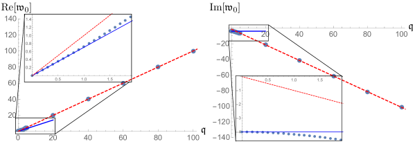
Figure 1: Comparison between numerical data and analytic results at high and low momentum for the lowest quasinormal mode of a massless scalar in the $z=d=2$ Lifshitz black brane background. The blue dots represent numerical data. The inset illustrates the small-$\mathfrak{q}$ dependence, where the blue line is the result in (117). The red line is the asymptotic large-$\mathfrak{q}$ result in (119).

5.2.2 Large-$\mathfrak{q}$ regime

From the data in Figure 1 it is evident that the quasinormal mode dependence on $\mathfrak{q}$ becomes linear in $\mathfrak{q}$ both for small $\mathfrak{q}$ and large $\mathfrak{q}.$ These two behaviours are, however, unrelated. As we have seen, the linearity in the small-$\mathfrak{q}$ regime is specific to the $z=d$ situation and contains information about the approach to equilibrium for slowly varying spatial anisotropy. The linearity at large $\mathfrak{q}$ is instead generic and occurs for all values of $(z,d).$

This can be verified analytically as well. In appendix C we provide a WKB calculation of the linear behaviour for asymptotically large values of $\mathfrak{q},$ including the leading off-set from linearity. The result for $z=d$ is given by

$$\mathfrak{w}_{n}=e^{-i\pi\frac{d-1}{2d}}\sqrt{\frac{d}{d-1}}(d-1)^{\frac{1}{2d}}\mathfrak{q}-\frac{id}{\sqrt{2}}(2n+1)+\mathcal{O}(\mathfrak{q}^{-1}).$$ (119)

Finally, it is interesting to note that the large-$\mathfrak{q}$ results imply that large-momentum excitations in a plasma dual to the Lifshitz-like black brane are always exponentially damped for $z>1.$ This is in stark contrast to the $z=1$ result, where regardless of the dimension, for asymptotically large $\mathfrak{q}$ the coefficient of the linear-in-$\mathfrak{q}$ term is exactly $\pm 1,$ indicating that high temperature CFT plasmas with holographic duals possess long-lived propagating excitations. In fact, in the $z=1$ case the WKB analysis is slightly more subtle and the overall structure is modified from the above such that the leading correction to the linear term is proportional to $\mathfrak{q}^{-\frac{d-1}{d+3}}$ and so becomes more suppressed as $\mathfrak{q}$ increases Festuccia:2008zx ; Fuini:2016qsc .

6 Non-equilibrium states

Up to now we have considered equilibrium states. Both in the $1+1$ CFT case and in the BTZ case it is possible to study the evolution of out of equilibrium states analytically for specific types of quenches. Here we extend those non-equilibrium results to the generalised quantum Lifshitz model and the holographic EMD theory for $z=d$.

6.1 States with translational and rotational symmetry

Autocorrelators in a general translationally and rotationally invariant state of the $z=d$ generalised quantum Lifshitz model are related to autocorrelators in a two-dimensional CFT. In the Heisenberg picture, the field operator equations of motion are solved by (in this section we work in real time)

$$\chi(x,t)=\int\frac{d^{d}p}{(2\pi)^{d}}\frac{1}{\sqrt{2\omega(p)}}\Big{(}e^{-i\omega(p)t+ip\cdot x}a_{p}+e^{i\omega(p)t-ip\cdot x}a_{p}^{\dagger}\Big{)},$$ (120)

where $\omega(p)=\kappa p^{d}$ and we denote $p^{d}\equiv(p^{2})^{\frac{d}{2}}$. The normalization of the operators $a_{p}$ and $a_{p}^{\dagger}$ is chosen so that they satisfy commutation relations $\left[a_{p},a^{\dagger}_{p^{\prime}}\right]=(2\pi)^{d}\delta^{d}(p-p^{\prime})$. The Wightman autocorrelator on a general Heisenberg picture state $|\psi\rangle$ is then given by

$$\langle\chi(t_{2})\chi(t_{1})\rangle=\int\frac{d^{d}p_{1}}{(2\pi)^{d}}\int\frac{d^{d}p_{2}}{(2\pi)^{d}}\frac{1}{2\sqrt{\omega(p_{1})\omega(p_{2})}}\Big{(}e^{-i\omega(p_{1})t_{1}-i\omega(p_{2})t_{2}}\langle a_{p_{2}}a_{p_{1}}\rangle$$

$$+e^{i\omega(p_{1})t_{1}-i\omega(p_{2})t_{2}}\langle a_{p_{2}}a_{p_{1}}^{\dagger}\rangle+e^{-i\omega(p_{1})t_{1}+i\omega(p_{2})t_{2}}\langle a_{p_{2}}^{\dagger}a_{p_{1}}\rangle+e^{i\omega(p_{1})t_{1}+i\omega(p_{2})t_{2}}\langle a_{p_{2}}^{\dagger}a_{p_{1}}^{\dagger}\rangle\Big{)}.$$ (121)

Assuming that the state $|\psi\rangle$ is invariant under spatial translation and rotation leads to the following form of the matrix elements of the creation and annihilation operators (a proof is given in Appendix D)

$$\langle a_{p_{2}}a_{p_{1}}\rangle=A_{11}(\omega(p_{1}))(2\pi)^{d}\delta^{d}(p_{1}+p_{2}),$$

$$\langle a_{p_{2}}a_{p_{1}}^{\dagger}\rangle=A_{12}(\omega(p_{1}))(2\pi)^{d}\delta^{d}(p_{1}-p_{2}),$$

$$\langle a_{p_{2}}^{\dagger}a_{p_{1}}\rangle=A_{21}(\omega(p_{1}))(2\pi)^{d}\delta^{d}(p_{1}-p_{2}),$$ (122)

$$\langle a_{p_{2}}^{\dagger}a_{p_{1}}^{\dagger}\rangle=A_{22}(\omega(p_{1}))(2\pi)^{d}\delta^{d}(p_{1}+p_{2}).$$

The two-point autocorrelator becomes

$$\langle\chi(t_{2})\chi(t_{1})\rangle=\int\frac{d^{d}p_{1}}{(2\pi)^{d}}\frac{1}{2\omega(p_{1})}\Big{(}e^{-i\omega(p_{1})(t_{1}+t_{2})}A_{11}(\omega(p_{1}))$$

$$+e^{i\omega(p_{1})(t_{1}-t_{2})}A_{12}(\omega(p_{1}))+e^{-i\omega(p_{1})(t_{1}-t_{2})}A_{21}(\omega(p_{1}))+e^{i\omega(p_{1})(t_{1}+t_{2})}A_{22}(\omega(p_{1}))\Big{)}.$$ (123)

Using the same change of integration variables as before $q=\kappa p_{1}^{d}$ and extending the integration region, we obtain

$$\langle\chi(t_{2})\chi(t_{1})\rangle=\frac{2\pi}{2^{d}\pi^{d/2}d\kappa\Gamma(\frac{d}{2})}\int\frac{dq}{2\pi}\frac{1}{2\bar{\omega}(q)}\Big{(}e^{-i\bar{\omega}(q)(t_{1}+t_{2})}A_{11}(\bar{\omega}(q))$$

$$+e^{i\omega(p_{1})(t_{1}-t_{2})}A_{12}(\bar{\omega}(q))+e^{-i\omega(q)(t_{1}-t_{2})}A_{21}(\bar{\omega}(q))+e^{i\omega(q)(t_{1}+t_{2})}A_{22}(\bar{\omega}(q))\Big{)},$$ (124)

where $\bar{\omega}(q)=|q|$. The autocorrelator (124) is identical to the autocorrelator of a 1+1 dimensional CFT with the action (39), now in Lorentzian time.

The state of a Gaussian CFT is specified by the matrix elements

$$\langle b_{q_{2}}b_{q_{1}}\rangle=A_{11}(\bar{\omega}(q_{1}))2\pi\delta(q_{1}+q_{2}),$$

$$\langle b_{q_{2}}b_{q_{1}}^{\dagger}\rangle=A_{12}(\bar{\omega}(q_{1}))2\pi\delta(q_{1}-q_{2}),$$

$$\langle b_{q_{2}}^{\dagger}b_{q_{1}}\rangle=A_{21}(\bar{\omega}(q_{1}))2\pi\delta(q_{1}-q_{2}),$$ (125)

$$\langle b_{q_{2}}^{\dagger}b_{q_{1}}^{\dagger}\rangle=A_{22}(\bar{\omega}(q_{1}))2\pi\delta(q_{1}+q_{2}),$$

where the creation and annihilation operators of the CFT satisfy the algebra $\left[b_{q},b^{\dagger}_{q^{\prime}}\right]=2\pi\delta(q-q^{\prime})$. We have so far demonstrated that the Wightman autocorrelators of the $z=d$ generalised quantum Lifshitz model are equivalent to the two-dimensional CFT Wightman autocorrelators. Other two-point correlation functions (such as Feynman or retarded correlators) can be obtained from linear combinations of Wightman functions and their complex conjugates. If the wavefunctional of the state $|\psi\rangle$ is Gaussian, one can obtain the correlation functions of all the composite operators, such as the monopole operators, by using Wick’s theorem with the $\langle\chi\chi\rangle$ two-point function. Thus, in Gaussian states with spatial translational and rotational symmetries, the autocorrelators of the generalised quantum Lifshitz model are identical to autocorrelators of a 1+1 dimensional free boson CFT.

6.2 A mass quench in the generalised quantum Lifshitz model

As a concrete example of a non-equilibrium state in the generalised quantum Lifshitz model with $z=d$, we can consider a quench state starting from the ground state of a different free Hamiltonian at $t=0$. In this case the matrix elements (122) are given by

$$A_{11}(\omega)=A_{22}=\frac{1}{4}\Big{(}\frac{\omega}{\omega_{0}}-\frac{\omega_{0}}{\omega}\Big{)},$$ (126)

$$A_{12}(\omega)=\frac{1}{4}\Big{(}\frac{\omega}{\omega_{0}}+\frac{\omega_{0}}{\omega}+2\Big{)},$$ (127)

$$A_{21}(\omega)=\frac{1}{4}\Big{(}\frac{\omega}{\omega_{0}}+\frac{\omega_{0}}{\omega}-2\Big{)},$$ (128)

where $\omega_{0}$ is the initial dispersion relation, and $\omega$ the final dispersion relation. These matrix elements can be computed from matching the initial and final ground state at $t=0$. In the case of a quench starting from the ground state of a mass deformed quantum Lifshitz Hamiltonian one has

$$\omega_{0}=\sqrt{\kappa^{2}p^{2d}+m_{0}^{2}},\quad\omega=\kappa p^{d}.$$ (129)

For simplicity we consider the case of a deep quench with $m_{0}^{-1}\ll t$ where $t$ is any of the following $|t_{1}-t_{2}|$, $t_{1}$ or $t_{2}$. This in particular gives the late time behaviour of the correlation function. The full time evolution of the correlator can be evaluated numerically. When $m_{0}$ is large, the leading contribution to the two-point function becomes

$$\langle\chi(t_{2})\chi(t_{1})\rangle\approx\frac{2\pi}{2^{d}\pi^{d/2}d\kappa\Gamma(\frac{d}{2})}\frac{m_{0}}{8\pi}\int_{0}^{\infty}\frac{dq}{q^{2}}\Big{(}e^{-iq(t_{2}-t_{1})}+e^{iq(t_{2}-t_{1})}-e^{-iq(t_{2}+t_{1})}-e^{iq(t_{2}+t_{1})}\Big{)},$$ (130)

where we use the integration variable $q=\kappa p^{d}$. Performing the integrals gives

$$\langle\chi(t_{2})\chi(t_{1})\rangle\approx\frac{2\pi}{2^{d}\pi^{d/2}d\kappa\Gamma(\frac{d}{2})}\frac{m_{0}}{8}\Big{(}t_{1}+t_{2}-|t_{2}-t_{1}|\Big{)}.$$ (131)

The Feynman propagator is given by

$$G_{F}(t_{2},t_{1})= \theta(t_{2}-t_{1})\langle\chi(t_{2})\chi(t_{1})\rangle+\theta(t_{1}-t_{2})\langle\chi(t_{1})\chi(t_{2})\rangle$$ (132)

$$\approx \frac{2\pi}{2^{d}\pi^{d/2}d\kappa\Gamma(\frac{d}{2})}\frac{m_{0}}{8}\Big{(}t_{1}+t_{2}-|t_{2}-t_{1}|\Big{)}.$$

The two-point function of monopole operators is obtained by using Wick’s theorem

$$\langle Te^{i\alpha\chi(t_{2})}e^{-i\alpha\chi(t_{1})}\rangle\approx e^{-\frac{\pi m_{0}}{2d}\Delta|t_{2}-t_{1}|}.$$ (133)

This has the same exponential fall off at large $|t_{2}-t_{1}|$ as the thermal autocorrelator if one identifies an effective temperature $T_{eff}=m_{0}/4$.

6.3 Vaidya collapse spacetime in the holographic model

A class of non-equilibrium states within holography is provided by “quenches” starting from the gapless ground state of the dual field theory. This can be achieved by introducing a time dependent source $J(t)$ for some operator in the dual field theory. A fast varying source induces a perturbation in some (combination of) field(s) close to the boundary of the space, which subsequently falls into the bulk and forms a black hole. Generically the time evolution has to be followed numerically by solving the dynamical Einstein’s equations coupled to whatever matter is present Gursoy:2016tgf . A simple metric that can be used to model the collapsing configuration is the Vaidya spacetime, which corresponds to null and pressureless matter sourcing Einstein’s equations.

An asymptotically Lifshitz version of the Vaidya spacetime was constructed in Keranen:2011xs and equal time correlators of scalar operators obtained in the geodesic approximation. Here we would instead like to consider autocorrelators in this time-dependent background.

For $z=d$ the Lifshitz-Vaidya spacetime is given by

$$ds^{2}=-\frac{1}{u^{2d}}\Big{(}1-m(v)u^{2d}\Big{)}dv^{2}-2\frac{dudv}{u^{d+1}}+\frac{d\textbf{x}^{2}}{u^{2}},$$ (134)

which can be transformed to the form

$$ds^{2}=\frac{1}{d^{2}}\frac{1}{y^{2}}\Big{[}-(1-d^{2}m(v)y^{2})dv^{2}-2dydv\Big{]}+\frac{1}{(dy)^{2/d}}d\textbf{x}^{2},$$ (135)

with the coordinate transformation $y=u^{d}/d$. The $g_{vv}$ and $g_{yv}$ components of the metric (135) are identical to those of the BTZ-Vaidya spacetime, and since the large-$\Delta$ limit of the autocorrelation function is insensitive to the $d\textbf{x}^{2}$ part of the metric, they will be identical to the autocorrelator in the BTZ-Vaidya background. These were computed in Balasubramanian:2012tu using the geodesic approximation in two different ways with the result

$$G_{F}(t_{2},t_{1})\propto\frac{1}{\Big{(}t_{1}\cosh(\pi Tt_{2})-\frac{1}{\pi T}\sinh(\pi Tt_{2})\Big{)}^{2\Delta/d}},$$ (136)

where $T$ is the temperature of the final state black hole. Due to the above reasoning, this is also the result for the non-equilibrium autocorrelator in the Lifshitz-Vaidya case as well. In (136) we have assumed $t_{1}<0$ and $t_{2}>0$. When both times are negative, i.e. before the collapse, the two-point function is instead identical to the vacuum one. Correspondingly, when both times are positive, i.e. after the collapse, the two-point function is identical to the thermal one.

7 Summary

In this paper we have studied two types of theories exhibiting a Lifshitz scale invariance: free field theories and holographic theories. The free field theories generalise the well known quantum Lifshitz model to arbitrary number of spatial dimensions. These theories can be defined for any value of $z$ but we restrict our attention for the most part to models with $z=d$ in order to retain some key properties of the original quantum Lifshitz model. In particular, precisely for $z=d$, one can define a set of scaling operators (so-called generalised monopole operators) whose equal time correlation functions match those of a $d$-dimensional conformal field theory. The holographic theories are dual to gravitational models of Einstein-Maxwell-dilaton (EMD) type and we consider scalar operators dual to massive scalar fields in the bulk geometry. By studying the vacuum and thermal correlation functions of these two classes of theories we have uncovered several interesting features.

At $z=d$ vacuum autocorrelation functions of scaling operators in the generalized quantum Lifshitz model can be expressed in terms of autocorrelators of a $1{+}1$-dimensional CFT. Likewise, for holographic models a similar relation manifests in the geodesic (or large-$\Delta$) approximation to the autocorrelator. This indicates an enhanced symmetry in the time domain that does not follow in an obvious way from the Lifshitz scaling symmetry. Furthermore, we find that the relation to a $1{+}1$-dimensional CFT persists when we consider autocorrelators in a thermal state. On the gravitational side we expect this finite temperature behaviour to be specific to the EMD models and that it will not persist in, for instance, Lifshitz models that are dual to bulk theories of Einstein-Proca form.

In the generalised quantum Lifshitz model the relation to autocorrelators in a $1{+}1$-dimensional CFT follows from a simple change of variables, $q=\kappa p^{d}$, in the momentum integrals in propagators. On the holographic side, the corresponding relation can be established by a transformation of the radial coordinate, $y=u^{d}/d$, which maps the $(u,t)$ section of the $z=d$ Lifshitz black brane metric to a corresponding $(y,t)$ section of a BTZ black hole metric. The relation to a $1{+}1$-dimensional CFT continues to hold for autocorrelators in out of equilibrium states of the generalised Lifshitz model that are invariant under spatial translations and rotations. Similarly, holographic non-equilibrium states described by a Lifshitz-Vaidya type collapsing spacetime can be mapped to the BTZ-Vaidya spacetime with the same coordinate transformation as in the thermal state. This leads to the equivalence between the large-$\Delta$ limit of autocorrelators in certain non-equilibrium states of holographic theories with Lifshitz scaling and $1{+}1$-dimensional CFTs with holographic duals.

We also consider correlation functions of operators with order one scaling dimensions, i.e. outside the geodesic approximation. In practice, we look for the poles of retarded thermal two-point functions, or in other words the quasinormal mode frequencies of the corresponding bulk fields. For zero spatial momentum, $p=0$, the quasinormal mode spectrum can be found analytically and agrees with the BTZ quasinormal mode spectrum. This again follows from the same coordinate transformation we used when evaluating autocorrelators. Furthermore, for large scaling dimension operators, the equal space limit of correlation functions can be argued to correspond to zero spatial momentum. Thus, we find consistent results with both methods. The quasinormal modes at small non-zero momenta also share features with the corresponding BTZ quasinormal modes. In particular, for $z=d$, we find that the frequency starts out purely real at low enough momentum and grows linearly with momentum, as in the BTZ case. At high momentum, on the other hand, we find interesting differences compared to CFT results. In particular, the imaginary part of the quasinormal mode frequency scales linearly with $p$ at high momentum. This is in strong contrast to holographic CFTs where the imaginary parts approach zero as $p^{-\frac{d-1}{d+3}}$ at high momentum. This implies that, while CFTs have long lived excitations at high momentum, we find that high momentum excitations are very short lived in Lifshitz theories with $z>1$. This has interesting implications for thermalisation of far from equilibrium configurations in these theories, which seems opposite to the pattern of thermalisation found in CFTs, where the long lived high momentum excitations are the slowest to equilibrate.

Appendix A Ground state wave functional in the generalised quantum Lifshitz model

The Hamiltonian of the generalised quantum Lifshitz model is given by

$$H=\frac{1}{2}\int d^{d}x\Big{(}\Pi(x)^{2}+\kappa^{2}(\nabla^{z}\chi)^{2}\Big{)},$$ (137)

where $\Pi(x)=\partial_{t}\chi$ is the canonical momentum, which in the Schrodinger picture is replaced by the operator

$$\Pi(x)=-i\frac{\delta}{\delta\chi(x)}.$$ (138)

The ground state of the theory can be found by solving the time independent Schrodinger equation

$$H\Psi\left[\chi\right]=E\Psi\left[\chi\right].$$ (139)

At this point if is convenient to introduce the operators

$$Q(x) =\frac{1}{\sqrt{2}}\Big{(}i\Pi(x)+\kappa(-\Box)^{z/2}\chi(x)\Big{)},$$ (140)

$$Q^{\dagger}(x) =\frac{1}{\sqrt{2}}\Big{(}-i\Pi(x)+\kappa(-\Box)^{z/2}\chi(x)\Big{)}.$$ (141)

The Hamiltonian can be now expressed as

$$H=\int d^{d}xQ^{\dagger}(x)Q(x)+E_{0},$$ (142)

where $E_{0}$ is given by

$$E_{0}=\lim_{x^{\prime}\rightarrow x}\int d^{d}x\frac{\kappa}{2}(-\Box)^{z/2}\delta^{d}(x-x^{\prime})=V_{d}\int\frac{d^{d}k}{(2\pi)^{d}}\frac{\omega(k)}{2},$$ (143)

where $\omega(k)=\kappa(k^{2})^{z/2}$. The operator $\tilde{H}=H-E_{0}$ is positive definite as for any normalizable state

$$\langle\tilde{H}\rangle=\int d^{d}x\langle\psi|Q^{\dagger}(x)Q(x)|\psi\rangle=\int d^{d}x||Q(x)|\psi\rangle||^{2}\geq 0.$$ (144)

Thus, if we can find a state for which $Q(x)|\psi\rangle=0$, this state will minimize the energy, i.e. it is the ground state of the theory. The equation

$$Q(x)\Psi\left[\chi\right]=\frac{1}{\sqrt{2}}\Big{(}\frac{\delta}{\delta\chi(x)}+\kappa(-\Box)^{z/2}\chi(x)\Big{)}\Psi\left[\chi\right]=0,$$ (145)

can be straightforwardly solved by

$$\Psi\left[\chi\right]=\frac{1}{\sqrt{Z}}e^{-\frac{1}{2}\int d^{d}x\chi(x)\kappa(-\Box)^{z/2}\chi(x)},$$ (146)

where $Z$ is a normalization factor that ensures the wavefunction has unit norm

$$Z=\int\left[d\chi\right]e^{-\kappa\int d^{d}x\chi(x)(-\Box)^{z/2}\chi(x)}.$$ (147)

Thus, the correlation functions of operators at equal time in the ground state are given by the expression

$$\langle\mathcal{O}(\chi)\rangle=\frac{1}{Z}\int\left[d\chi\right]e^{-\kappa\int d^{d}x\chi(x)(-\Box)^{z/2}\chi(x)}\mathcal{O}(\chi),$$ (148)

which can be identified as a correlation functions in a $d$-dimensional Euclidean CFT if $z=d$.

Appendix B Generic two-point function at $z=2$

We want to compute a two-point function in the geodesic approximation with both spatial and temporal dependence. For $z=2$ we can allow for arbitrary values of both $E$ and $p$. In this case (65) gives

$$u^{2}=\frac{4e^{2\lambda}}{1+2e^{2\lambda}p^{2}+e^{4\lambda}(p^{4}+4E^{2})},$$ (149)

and is is easy to see that (66) and (70) are recovered by setting $E=0$ or respectively $p=0$ and shifting the affine parameter by a constant. At the endpoints of the regularized geodesic, where $u=\epsilon$, the affine parameter takes the values

$$\lambda_{1}=-\log\frac{\epsilon}{2}-\frac{1}{2}\log(p^{4}+4E^{2})+O(\epsilon^{2})\,,\qquad\lambda_{2}=\log\frac{\epsilon}{2}+O(\epsilon^{2})\,,$$ (150)

and the regularized length is given by

$$L_{R}=-2\log\frac{\epsilon}{2}-\frac{1}{2}\log(p^{4}+4E^{2})+O(\epsilon^{2})\,.$$ (151)

Inserting this into (58) leads to a simple expression for the vacuum two-point function of scaling operators in terms of $p$ and $E$,

$$\langle\mathcal{O}^{R}(\vec{x}_{1},\tau_{1})\mathcal{O}^{R}(\vec{x}_{2},\tau_{2})\rangle=\left(\Big{(}\frac{p}{2}\Big{)}^{4}+\Big{(}\frac{E}{2}\Big{)}^{2}\right)^{\Delta/2}.$$ (152)

Integrating the conservation laws (62) and (63) gives

$$|\tau_{12}| = \frac{1}{E}\left(1-\frac{\eta}{\tan\eta}\right)\,,$$ (153)

$$|\vec{x}_{12}| = \frac{2}{p}\,\frac{\eta}{\tan\eta}\,.$$ (154)

where the scaling variable $\eta$ is defined via

$$\frac{2E}{p^{2}}=\tan\eta\,,$$ (155)

or equivalently

$$\frac{|\vec{x}_{12}|^{2}}{|\tau_{12}|}=\frac{2\eta^{2}}{\tan\eta-\eta}\,.$$ (156)

This can in principle be inverted to obtain $\eta$ as a function of $|\vec{x}_{12}|^{2}/|\tau_{12}|$.

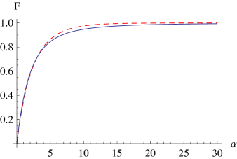
Figure 2: The blue (solid) curve shows the scaling function that appears in the holographic two-point function, while the red (dashed) curve shows the corresponding scaling function found for two-point functions of monopole operators in the quantum Lifshitz model. Both are plotted as functions of the scaling variable $\alpha=|\vec{x}_{12}|^{2}/|\tau_{12}|$.

The vacuum two-point correlation function (152) can be expressed in terms of the scaling variable in two equivalent ways,

$$\langle\mathcal{O}^{R}(\vec{x}_{1},\tau_{1})\mathcal{O}^{R}(\vec{x}_{2},\tau_{2})\rangle=\frac{F(\eta)^{\Delta}}{|\vec{x}_{12}|^{2\Delta}}=\frac{\tilde{F}(\eta)^{\Delta}}{|2\tau_{12}|^{\Delta}}\,,$$ (157)

with

$$F(\eta)=\frac{\eta^{2}\cos\eta}{\sin^{2}\eta}\qquad\textrm{and}\qquad\tilde{F}(\eta)=\frac{1}{\sin\eta}\Big{(}1-\frac{\eta\cos\eta}{\sin\eta}\Big{)}\,.$$ (158)

We can obtain series expansions for the two-point function in different asymptotic limits by using the relation (156). The limit $|\vec{x}_{12}|^{2}\gg|\tau_{12}|$ corresponds to $\eta\rightarrow 0$ and

$$\langle\mathcal{O}^{R}(\vec{x}_{1},\tau_{1})\mathcal{O}^{R}(\vec{x}_{2},\tau_{2})\rangle=\frac{1}{|\vec{x}_{12}|^{2\Delta}}\left(1-6\Delta\frac{|\tau_{12}|^{2}}{|\vec{x}_{12}|^{4}}+\ldots\right),$$ (159)

which reduces to the equal time result (69) when $|\tau_{12}|\rightarrow 0$. On the other hand, $|\tau_{12}|\gg|\vec{x}_{12}|^{2}$ amounts to $\eta\rightarrow\pi/2$ and

$$\langle\mathcal{O}^{R}(\vec{x}_{1},\tau_{1})\mathcal{O}^{R}(\vec{x}_{2},\tau_{2})\rangle=\frac{1}{|2\tau_{12}|^{\Delta}}\left(1-\frac{\Delta}{\pi}\frac{|\vec{x}_{12}|^{2}}{|\tau_{12}|}+\ldots\right),$$ (160)

which in turn reduces to the autocorrelator (72) for $z=2$ when $|\vec{x}|\rightarrow 0$.

The corresponding two-point function can be straightforwardly calculated in the original quantum Lifshitz model (see e.g. Ardonne:2003wa , or our Section 2.2). In the limit $|\vec{x}|^{2}\gg\kappa|\tau_{12}|$ one finds

$$\langle\mathcal{O}^{R}(\vec{x}_{1},\tau_{1})\mathcal{O}^{R}(\vec{x}_{2},\tau_{2})\rangle_{\textrm{QL}}=\frac{1}{|\vec{x}_{12}|^{2\Delta}}\left(1-\frac{4\Delta\kappa|\tau_{12}|}{|\vec{x}_{12}|^{2}}e^{-\frac{|\vec{x}_{12}|^{2}}{4\kappa|\tau_{12}|}}+\ldots\right),$$ (161)

while the leading behaviour for $|\vec{x}_{12}|^{2}\ll\kappa|\tau_{12}|$ is

$$\langle\mathcal{O}^{R}(\vec{x}_{1},\tau_{1})\mathcal{O}^{R}(\vec{x}_{2},\tau_{2})\rangle_{\textrm{QL}}=\frac{1}{|2\kappa\tau_{12}|^{\Delta}}\left(1-\frac{\Delta}{4}\frac{|\vec{x}_{12}|^{2}}{\kappa|\tau_{12}|}+\ldots\right).$$ (162)

The holographic two-point function and the one found in the quantum Lifshitz model agree in the special cases when either $|\tau_{12}|=0$ or $|\vec{x}_{12}|=0$ and they both exhibit scaling in $|\vec{x}_{12}|^{2}/|\tau_{12}|$ at generic separation, but the scaling functions differ in the two theories. In particular, the approach to the equal-time result is exponentially fast in the quantum Lifshitz model but power law in the holographic model. The scaling functions are compared in Figure 2 where we compare (158) and (28) when plotted against $\alpha\equiv|\vec{x}_{12}|^{2}/|\tau_{12}|$.

Appendix C Quasinormal mode spectrum

In this appendix we provide some details on the computation of the quasinormal mode spectrum. In particular, we elaborate on our numerical procedure as well as obtain analytical results for small-$\mathfrak{q}$ in (117) and large-$\mathfrak{q}$ in (119).

C.1 Numerical Algorithm

To perform the numerical computation we used the Mathematica package “QNMspectral” Jansen . The essence of the algorithm boils down to the following. First we cast the scalar wave equation (55) in infalling Eddington-Finkelstein coordinates with a compact radial coordinate, which we discretise on a spectral grid. This grid puts more points near the boundary and horizon than in the “middle”, which is convenient for numerical purposes. We then express the eigenfunctions in terms of a sum of Chebychev polynomials where we take into account the required fall-off. Note that we can only have as many Chebychev coefficients as points on the spectral grid. This yields a set of equations which can be cast into the form of a generalised eigenvalue problem,

$$M\cdot\vec{v}=\omega\cdot\vec{v}\,,$$ (163)

where $\vec{v}$ is a vector with the coefficients of the Chebychev expansion and $M$ is a matrix with values depending on the details of the quasinormal mode equation (55). The eigenvalue problem can readily be solved using Mathematica. In principle, the higher rank the matrix $M$, the higher the precision and number of overtone numbers $n$ of the quasinormal modes $\omega$. The minimum numerical precision of the quasinormal modes computed in this paper is better than 1%.

C.2 Small-$\mathfrak{q}$ expansion

In order to derive (117) we begin with the the scalar wave equation in the $z=d$ Lifshitz black brane background (107), which we rewrite here for completeness

$$\varphi^{\prime\prime}(\mathfrak{u})-\frac{1}{1-\mathfrak{u}}\varphi^{\prime}(\mathfrak{u})+\frac{1}{4\mathfrak{u}^{2}(1-\mathfrak{u})d^{2}}\left(\frac{\mathfrak{w}^{2}\mathfrak{u}}{(1-\mathfrak{u})}-\mathfrak{q}^{2}\mathfrak{u}^{\frac{1}{d}}-\Delta(\Delta-2d)\right)\varphi(\mathfrak{u})=0\,.$$ (164)

For $\mathfrak{q}=0,$ solution that is regular at infinity is given by (110) with $\varphi_{-}=0,$ such that

$$\varphi(\mathfrak{u})=\varphi_{+}\,\mathfrak{u}^{\frac{\Delta_{+}}{2d}}(1-\mathfrak{u})^{-\frac{i\mathfrak{w}}{2d}}{}_{2}F_{1}\left({\textstyle\frac{\Delta_{+}}{2d}}-{\textstyle\frac{i\mathfrak{w}}{2d}},{\textstyle\frac{\Delta_{+}}{2d}}-{\textstyle\frac{i\mathfrak{w}}{2d}},{\textstyle\frac{\Delta_{+}}{d}},\mathfrak{u}\right).$$ (165)

Imposing in-falling boundary conditions at the horizon further restricts the solution such that $\mathfrak{w}$ is quantized as

$$\mathfrak{w}_{n,\mathfrak{q}=0}=-i(\Delta+2nd),\qquad n=0,\,1,\,2,\cdots.$$ (166)

For generic values of $\mathfrak{w}$ the hypergeometric function in (165) is given by an infinite series in $\mathfrak{u},$ however at the quasinormal values of $\mathfrak{w}$ in (166) the series terminates and one can write the hypergeometric as a finite degree polynomial. In particular, when evaluated on the quasinormal frequency the $\mathfrak{q}=0$ scalar solution is (see eq. 15.4.1 of AbramowitzStegun )

$$\varphi(\mathfrak{u}) = \varphi_{+}\,\mathfrak{u}^{\frac{\Delta_{+}}{2d}}(1-\mathfrak{u})^{-n-\frac{\Delta}{2d}}{}_{2}F_{1}\left(-n,-n,{\textstyle\frac{\Delta_{+}}{d}},\mathfrak{u}\right)$$ (167)

$$= \varphi_{+}\,\mathfrak{u}^{\frac{\Delta_{+}}{2d}}(1-\mathfrak{u})^{-n-\frac{\Delta}{2d}}\sum_{m=0}^{n}\frac{(-n)_{m}^{2}}{m!({\textstyle\frac{\Delta}{d}})_{m}}\mathfrak{u}^{m},$$

where the Pochhammer symbol $(\cdot)_{m}$ is defined by

$$(a)_{m}\equiv\frac{\Gamma(a+m)}{\Gamma(a)}.$$ (168)

We will now specialize to the case $n=0$ and will come back to the generic-$n$ situation later. At $n=0$ the hypergeometric function above is a constant. In order to find the momentum dependence we then make the following ansatz

$$\varphi(\mathfrak{u})=\mathfrak{u}^{\frac{\Delta}{2d}}(1-\mathfrak{u})^{-\frac{\Delta}{2d}-i\frac{\hat{\mathfrak{w}}}{2d}}\hat{\varphi}(\mathfrak{u}),$$ (169)

where $\hat{\varphi}(\mathfrak{u})$ parametrizes the deviation from the $\mathfrak{q}=0$ solution and we have set $\mathfrak{w}=-i\Delta+\hat{\mathfrak{w}}$, so that $\hat{\mathfrak{w}}$ is the shift of the frequency from the $\mathfrak{q}=0$ result. Its appearance in the exponent above is required by the in-falling boundary condition at the horizon.

Inserting this into (107) we find the following equation for $\hat{\phi}(\mathfrak{u})$

$$\left(\mathfrak{u}^{\frac{\Delta}{d}}(1-\mathfrak{u})^{1-\frac{\Delta}{d}}\hat{\varphi}^{\prime}(\mathfrak{u})\right)^{\prime}+\frac{i\hat{\mathfrak{w}}\mathfrak{u}^{\frac{\Delta}{d}}}{d(1-\mathfrak{u})^{\frac{\Delta}{d}}}\hat{\varphi}^{\prime}(\mathfrak{u})+\frac{\mathfrak{u}^{\frac{\Delta}{d}-2}}{4d^{2}(1-\mathfrak{u})^{\frac{\Delta}{d}}}(\mathfrak{u}\hat{\mathfrak{w}}^{2}-\mathfrak{u}^{\frac{1}{d}}\mathfrak{q}^{2})\hat{\varphi}(\mathfrak{u})=0.$$ (170)

Solving this equation perturbatively in $\hat{\mathfrak{w}}$ and $\mathfrak{q}$, and demanding regularity at the boundary $\mathfrak{u}\rightarrow 0$, one finds that the solution up to $\mathcal{O}(\hat{\mathfrak{w}}^{2},\mathfrak{q}^{2})$ is given by

$$\hat{\phi}(\mathfrak{u})=$$

$$\phi_{0}\Bigg{[}1-\frac{\Gamma(1-\frac{\Delta}{d})}{4d\Gamma(\frac{1}{d})}\int d\mathfrak{u}^{\prime}\mathfrak{u}^{\prime-\frac{\Delta}{d}}(1-\mathfrak{u}^{\prime})^{\frac{\Delta}{d}-1}\left(\Gamma(1+{\textstyle\frac{\Delta}{d}})\Gamma({\textstyle\frac{1}{d}})\hat{\mathfrak{w}}^{2}-\frac{\Delta}{\Delta+1-d}\Gamma({\textstyle\frac{\Delta+1}{d}})\mathfrak{q}^{2}\right)$$

$$-\int\frac{d\mathfrak{u}^{\prime}}{4d(\Delta-d)}\left(\hat{\mathfrak{w}}^{2}F(1,1,2-{\textstyle\frac{\Delta}{d}},1-\mathfrak{u}^{\prime})-\mathfrak{q}^{2}\mathfrak{u}^{\frac{1}{d}-1}F({\textstyle\frac{1}{d}},1,2-{\textstyle\frac{\Delta}{d}},1-\mathfrak{u}^{\prime})\right)\Bigg{]}+\mathcal{O}(\hat{\mathfrak{w}}^{3},\mathfrak{q}^{3}).$$

The important point to note for our purposes is that, when $\frac{\Delta}{d}$ is not an integer, the integral on the first line gives a solution which is non-analytic at $\mathfrak{u}=1$ and should be vanishing. In order for this term to vanish one must set

$$\hat{\mathfrak{w}}^{2}=\frac{\Gamma(\frac{\Delta+1-d}{d})}{\Gamma(\frac{\Delta}{d})\Gamma(\frac{1}{d})}\mathfrak{q}^{2},$$ (171)

which is the result quoted in (117). One can perform the same analysis with the generic form of the quasinormal solution in (167) to obtain the general-$n$ result,

$$\hat{\mathfrak{w}}^{2}=\frac{\Gamma\left(n+\frac{\Delta}{d}\right)^{2}}{\Gamma(n+1)^{2}\Gamma\left(\frac{\Delta}{d}\right)^{2}\Gamma\left(2n+\frac{\Delta}{d}\right)}\sum_{i,j=0}^{n}\frac{(-n)^{2}_{i}}{\left(\frac{\Delta}{d}\right)_{i}}\frac{1}{i!}\frac{(-n)^{2}_{j}}{\left(\frac{\Delta}{d}\right)_{j}}\frac{1}{j!}\frac{\Gamma\left[i+j+\frac{\Delta}{d}+\frac{1}{d}-1\right]}{\Gamma\left[i+j+\frac{1}{d}-2n\right]}\mathfrak{q}^{2}\,.$$ (172)

C.3 Large-$\mathfrak{q}$ WKB

At high momentum, we can compute the scalar mode functions in a WKB approximation that is valid for large $\mathfrak{q}.$ using a method described in Festuccia:2008zx . We will carry out the calculation using generic values of $(d,z)$ and later specialize to the case of $d=z.$

In order to set notation, let us write the metric for generic $(d,z)$

$$ds^{2}=\frac{f(u)}{u^{2z}}d\tau^{2}+\frac{du^{2}}{u^{2}f(u)}+\frac{d\textbf{x}^{2}}{u^{2}},\quad f(u)=1-\frac{u^{d+z}}{u_{H}^{d+z}}.$$ (173)

The scalar wave equation for generic $(d,z)$ is given by

$$\varphi^{\prime\prime}(\mathfrak{u})-\frac{1}{1-\mathfrak{u}}\varphi^{\prime}(\mathfrak{u})+\frac{1}{\mathfrak{u}^{2}(1-\mathfrak{u})(d+z)^{2}}\left(\frac{\mathfrak{w}^{2}\mathfrak{u}^{\frac{2z}{d+z}}}{(1-\mathfrak{u})}-\mathfrak{q}^{2}\mathfrak{u}^{\frac{2}{z+d}}-m^{2}\right)\varphi(\mathfrak{u})=0,$$ (174)

where we have again defined dimensionless quantities, which for generic $(d,z)$ are now given by

$$\mathfrak{u} = \frac{u^{d+z}}{u_{H}^{d+z}},$$

$$\mathfrak{w} = \left(\frac{4\pi T}{d+z}\right)^{-1}\omega,$$

$$\vec{\mathfrak{q}} = \left(\frac{4\pi T}{d+z}\right)^{-1/z}\vec{p}\,.$$ (175)

and

$$m^{2}=\Delta(\Delta-d-z).$$ (176)

It is useful to write the wave equation in terms of the so-called “tortoise” coordinate, which we define to be

$$r_{\star}=\frac{1}{d+z}\int_{0}^{\mathfrak{u}}\mathfrak{u}^{\prime-\frac{d}{d+z}}\frac{d\mathfrak{u}^{\prime}}{1-\mathfrak{u}^{\prime}}.$$ (177)

With this convention the boundary is located at $r_{\star}=0$ and the horizon is approached as $r_{\star}\rightarrow\infty.$

In terms of the rescaled wave function $\psi(\mathfrak{u})=\mathfrak{u}^{-\frac{d}{2(d+z)}}\varphi(\mathfrak{u})$, the equation of motion (174) can be written in Schrödinger form

$$(-\partial_{r_{\star}}^{2}+V(\mathfrak{u}))\psi=\mathfrak{w}^{2}\psi,$$ (178)

where the potential is given by

$$V(\mathfrak{u})=\frac{1-\mathfrak{u}}{\mathfrak{u}^{\frac{2z}{d+z}}}\left[\mathfrak{q}^{2}\mathfrak{u}^{\frac{2}{d+z}}+\nu^{2}-\frac{z^{2}}{4}+\frac{d^{2}}{4}\mathfrak{u}\right],$$ (179)

with $\nu^{2}=m^{2}-\frac{(d+z)^{2}}{4}.$ To take the large $\mathfrak{q}$ limit, we rescale the frequency as

$$\mathfrak{w}=w\mathfrak{q},$$ (180)

in which case the equation of motion can be solved in an expansion in inverse powers of $\mathfrak{q}.$ In particular, we can write the potential as

$$V(\mathfrak{u})=\mathfrak{q}^{2}V_{0}(\mathfrak{u})+V_{2}(\mathfrak{u}),$$ (181)

where

$$V_{0}(\mathfrak{u})=\mathfrak{u}^{\frac{2(1-z)}{d+z}}(1-\mathfrak{u}).$$ (182)

To determine the leading WKB quasinormal modes, we only need to take into account the leading order potential $V_{0}(\mathfrak{u})$. The additional terms in $V_{2}(\mathfrak{u})$ yield sub-leading contributions that are suppressed by powers of $\mathfrak{q}^{-1}$.

In what follows, we will review the analysis of Festuccia:2008zx . It is important to note that for $z>1$ the potential in (182) behaves very differently near the boundary compared to the case of $z=1$ studied in Festuccia:2008zx . In particular, for $z=1$ (182) approaches a constant at the boundary, whereas for $z>1$ it diverges. This divergence will naturally lead to bound state solutions. The following analysis will therefore echo the large-mass analysis of Festuccia:2008zx , rather than the high momentum analysis.

First, consider the situation for real values of $w$, in which case intuition from one-dimensional scattering in quantum mechanics is useful. In particular, since the potential vanishes at the horizon $u=1,$ the function

$$\kappa(r_{\star})=w^{2}-V_{0}(r_{\star})$$ (183)

is positive for sufficiently large $r_{\star}$ as one approaches the horizon. The WKB solutions in this region correspond to oscillating waves

$$\psi_{>,\pm}(r_{\star})=\frac{A_{>,\pm}}{\kappa(r_{\star})^{1/4}}e^{\pm i\mathfrak{q}W(r_{\star})}+\mathcal{O}(\mathfrak{q}^{-1})\,,$$ (184)

where

$$W(r_{\star})\equiv\int_{r_{\star c}}^{r_{\star}}dr_{\star}^{\prime}\sqrt{w^{2}-V_{0}(\mathfrak{u}(r_{\star}^{\prime}))}$$ (185)

and $r_{\star c}$ corresponds to a classical turning point of the potential, such that $\kappa(r_{\star c})=0.$

As one moves further from the horizon eventually $r_{\star}=r_{\star c}$, after which one enters the classically forbidden region with $\kappa(r_{\star})<0$. The WKB solutions in this region correspond to rising and falling exponentials

$$\psi_{<,\pm}(r_{\star})=\frac{A_{<,\pm}}{(-\kappa(r_{\star}))^{1/4}}e^{\pm\mathfrak{q}\mathcal{Z}(r_{\star})}+\mathcal{O}(\mathfrak{q}^{-1})\,,$$ (186)

where

$$\mathcal{Z}(r_{\star})\equiv\int_{r_{\star c}}^{r_{\star}}dr_{\star}^{\prime}\sqrt{V_{0}(r_{\star}^{\prime})-w^{2}}.$$ (187)

Writing the integral out explicitly in terms of the coordinate $\mathfrak{u},$

$$\mathcal{Z}(u)=\frac{1}{d+z}\int_{\mathfrak{u}_{c}}^{\mathfrak{u}}d\mathfrak{u}^{\prime}\frac{1}{1-\mathfrak{u}^{\prime}}\mathfrak{u}^{\prime-\frac{d}{d+z}}\sqrt{V_{0}(\mathfrak{u}^{\prime})-w^{2}},$$ (188)

where $\mathfrak{u}<\mathfrak{u}_{c},$ we see that $\mathcal{Z}(\mathfrak{u})$ is negative and decreasing as $\mathfrak{u}$ moves away from the turning point and so the solution $\psi_{<,+}(r_{\star})$ corresponds to the decaying mode under the potential barrier. As one further approaches the boundary at $r_{\star}=0$ the WKB solutions behave as

$$\psi_{<,\pm}(\mathfrak{u})\simeq A_{<,\pm}e^{\pm\mathfrak{q}\mathcal{Z}(r_{\star c},0)}\mathfrak{u}^{\frac{(z-1)}{2(d+z)}}e^{\pm\mathfrak{q}\mathfrak{u}^{\frac{1}{d+z}}}.$$ (189)

In order to construct quasinormal solutions we will build the solution up from the boundary. Near the boundary, the WKB expansion breaks down and one must solve for the wave-function in a near-boundary expansion. At large-$\mathfrak{q}$, the $w^{2}$ term is suppressed by powers of $\mathfrak{q}^{-1}$ and the near-boundary solution is independent of $w$ to lowest order. The regular solution near the boundary is given by

$$\psi_{n.b.}(u)=B\,\mathfrak{u}^{\frac{z}{2(d+z)}}I_{\nu}(\mathfrak{q}\mathfrak{u}^{\frac{1}{d+z}}),$$ (190)

which scales as $\phi\sim u^{\nu+(d+z)/2}$ for small $u$ as is appropriate for a normalizable mode. To match this to the WKB solutions in (186) we expand for large $\mathfrak{u},$

$$\psi_{n.b.}(u)\simeq B\,\frac{\mathfrak{u}^{\frac{z-1}{2(d+z)}}}{\sqrt{2\pi\mathfrak{q}}}e^{\mathfrak{q}\mathfrak{u}^{\frac{1}{d+z}}}.$$ (191)

We therefore see that the normalizable solution at the boundary can be matched onto the decaying WKB solution $\psi_{<,+}(r_{\star}),$ with $A_{<,-}=0$ and

$$B=\sqrt{2\pi\mathfrak{q}}e^{\mathfrak{q}\mathcal{Z}(r_{\star c},0)}A_{<,+}.$$ (192)

Next, matching the solution $\psi_{<,+}(r_{\star})$ across the turning point onto the oscillating solutions in (184) one finds the solution in the allowed region ($r_{\star}>r_{\star c}$) to have $A_{>,-}=e^{i\pi/2}A_{>,+},$ such that

$$\psi(r_{\star})=\frac{2A_{>,+}}{\kappa(r_{\star})^{1/4}}\cos\left(\mathfrak{q}W(r_{\star})-\frac{\pi}{4}\right),\qquad r_{\star}>r_{\star c}.$$ (193)

For large $r_{\star}$ this solution behaves as a linear combination of $e^{+i\mathfrak{q}r_{\star}}$ and $e^{-i\mathfrak{q}r_{\star}}.$ The first behaviour corresponds to an in-falling wave and the latter to an out-going wave. Solutions with real $w$ are therefore not quasinormal.

To find quasinormal frequencies one must analytically continue by allowing both $w$ and $r_{\star}$ to take complex values. This allows for additional turning points where $\kappa(r_{\star})$ vanishes. In particular, there will be special complex values of $w$ where one of these new turning points, which we will refer to as $r_{\star t},$ will merge with the analytic continuation of the physical turning point $r_{\star c}.$ As explained in Festuccia:2008zx , when this occurs certain sub-dominant contributions to the out-going mode will become of the same order as the leading term. Near the point where the turning points merge, the ratio of the two contributions to the out-going mode is given by

$$e^{2\mathfrak{q}\mathcal{Z}(r_{\star c},r_{\star t})},$$ (194)

where

$$\mathcal{Z}(r_{\star c},r_{\star t})=\int_{r_{\star c}}^{r_{\star t}}dr_{\star}^{\prime}\sqrt{V_{0}(r_{\star}^{\prime})-w^{2}}.$$ (195)

This means that when

$$e^{2\mathfrak{q}\mathcal{Z}(r_{\star c},r_{\star t})}=-1,$$ (196)

the two contributions will exactly cancel and leads to the quantization condition Festuccia:2008zx

$$2\mathfrak{q}\mathcal{Z}(r_{\star c},r_{\star t})=i\pi(2n+1),\qquad n=0,\,1,\,2,\,\cdots.$$ (197)

The two turning points merge when the following two conditions are satisfied,

$$V_{0}(\mathfrak{u}_{b}) = w_{b}^{2},$$

$$V_{0}^{\prime}(\mathfrak{u}_{b}) = 0,$$ (198)

which ensure that $\kappa(r_{\star})$ has a second order zero at $r_{\star b}\equiv r_{\star}(u_{b}).$ We can approximate the potential around the point where the two turning points merge as a quadratic polynomial

$$V_{0}(r_{\star})\simeq V_{0}(r_{\star b})+\frac{1}{2}V_{0}^{\prime\prime}(r_{\star b})(r_{\star}-r_{\star b})^{2}.$$ (199)

Furthermore, assuming $w=w_{b}+x,$ where $x$ is small, we see that the turning points $r_{\star t}$ and $r_{\star c}$ are located at $r_{\star b}\pm a,$ where

$$a=\sqrt{\frac{4w_{b}x}{V_{0}^{\prime\prime}(r_{\star b})}}.$$ (200)

In this approximation we can perform the integral

$$\mathcal{Z}(r_{\star c},r_{\star t}) = \int_{r_{\star c}}^{r_{\star t}}dr_{\star}^{\prime}\sqrt{V_{0}(r_{\star}^{\prime})-w^{2}}$$ (201)

$$\simeq \int_{-a}^{a}dy\sqrt{{\textstyle\frac{1}{2}}V_{0}^{\prime\prime}(r_{\star b})y^{2}-2xw_{b}}$$

$$\simeq \pm ia^{2}\sqrt{\frac{V_{0}^{\prime\prime}(r_{\star b})}{2}}\int_{-1}^{1}dy\sqrt{1-y^{2}}$$

$$\simeq \pm i\frac{a^{2}\pi}{2}\sqrt{\frac{V_{0}^{\prime\prime}(r_{\star b})}{2}}$$

$$\simeq \pm\frac{i\pi x}{\delta},$$

where

$$\delta=\sqrt{\frac{V_{0}^{\prime\prime}(r_{\star})}{2V_{0}(r_{\star})}}\Big{|}_{r_{\star}=r_{\star b}}.$$ (202)

The quantization condition (197) then leads to the expression

$$w_{n} = w_{b}+x$$ (203)

$$= w_{b}+\frac{\delta}{2\mathfrak{q}}(2n+1).$$

The quasinormal frequencies are then given by

$$\mathfrak{w}=\mathfrak{q}w_{b}+\frac{\delta}{2}(2n+1),\qquad n=0,\,1,\,2,\,\cdots.$$ (204)

Evaluating this for our potential in (182), we find the turning point conditions to be

$$\mathfrak{u}_{b} = -\frac{2(z-1)}{d+2-z},$$

$$w_{b} = e^{-i\pi\frac{(z-1)}{d+z}}\sqrt{\frac{d+z}{d+2-z}}\left(\frac{2(z-1)}{d+2-z}\right)^{-\frac{(z-1)}{d+z}}.$$ (205)

Evaluating the offset $\delta$ in (202) for this case we find

$$\delta=e^{-i\pi\frac{z}{d+z}}\frac{d+z}{\sqrt{2}}\left(\frac{2(z-1)}{d+2-z}\right)^{\frac{d-z}{2(d+z)}}.$$ (206)

Note that we only trust these results for $z$ in the range $1<z<d+2.$ The case of $z\geq d+2$ needs to be treated with more care as the point $u_{b}$, where the turning points merge, goes behind the horizon, i.e. $\mathfrak{u}_{b}>1$.

For the case of $d=z,$ this gives the following result for the quasinormal frequencies

$$\mathfrak{w}_{n}=e^{-i\pi\frac{d-1}{2d}}\sqrt{\frac{d}{d-1}}(d-1)^{\frac{1}{2d}}\mathfrak{q}-\frac{id}{\sqrt{2}}(2n+1)+\mathcal{O}(\mathfrak{q}^{-1}).$$ (207)

Figure 3 provides an overview of our numerical results for several values of $d$, $z$ and $\mathfrak{q}$.

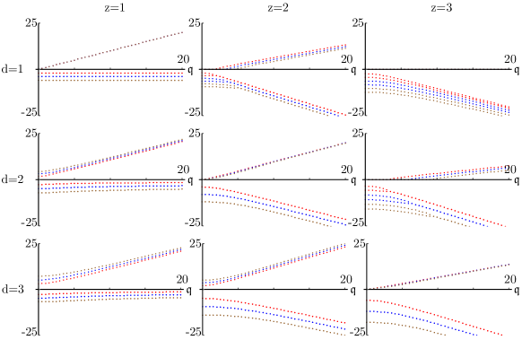
Figure 3: Real and imaginary parts of the first three overtones ($n=0,1,2$) in the EMD model for a massless field with $\Delta=d+z$. The dots above the x-axis represent the real part and the ones below the axis represent the imaginary part. Notice the different behaviour at small $\mathfrak{q}$ when $d>z$, $d=z$ or $d<z$. In the $d=1$ and $z=3$ plot, the real parts remain zero, as expected from the large-$\mathfrak{q}$ WKB result.

Appendix D Matrix elements of creation and annihilation operators

In this Appendix we demonstrate how the momentum dependence of the creation and annihilation operator matrix elements (122) is fixed by rotational and translational invariance of the state $|\psi\rangle$. The vacuum $|0\rangle$ is a state invariant under rotations and translations

$$e^{ix\cdot P}|0\rangle=|0\rangle,\quad U(R)|0\rangle=|0\rangle,$$ (208)

where $P$ is the momentum operator and $U(R)$ is an operator generating the rotation $R$. The one particle state $|p\rangle=a^{\dagger}_{p}|0\rangle$ transforms as

$$e^{ix\cdot P}|p\rangle=e^{ix\cdot p}|p\rangle,\quad U(R)|p\rangle=|Rp\rangle,$$ (209)

where $(Rp)^{i}=R^{i}_{j}p^{j}$ is the rotated momentum. This leads to the following transformation properties of the creation operators

$$e^{ix\cdot P}a_{p}^{\dagger}e^{-ix\cdot P}=a_{p}^{\dagger}e^{ix\cdot p},\quad U(R)a_{p}^{\dagger}U^{\dagger}(R)=a_{Rp}^{\dagger}.$$ (210)

The transformation properties of the annihilation operators follow from Hermitian conjugation. Next we consider one of the matrix elements in (122)

$$f(p_{1},p_{2})=\langle\psi|a_{p_{1}}a_{p_{2}}|\psi\rangle.$$ (211)

We assume that the state $\psi$ is invariant under translations and rotations, $e^{ix\cdot P}|\psi\rangle=|\psi\rangle$ and $U(R)|\psi\rangle=|\psi\rangle$. Inserting three unit operators $1=U^{\dagger}(R)U(R)$ in (211) gives

$$f(p_{1},p_{2})=f(Rp_{1},Rp_{2}),$$ (212)

which means that $f(p_{1},p_{2})$ is a function of the rotationally invariant combinations $p_{1}^{2}$, $p_{2}^{2}$ and $p_{1}\cdot p_{2}$. By inserting three unit operators $1=e^{-ix\cdot P}e^{ix\cdot P}$ in (211) gives

$$f(p_{1},p_{2})=e^{ix\cdot(p_{1}+p_{2})}f(p_{1},p_{2}).$$ (213)

Since $f(p_{1},p_{2})$ should be independent of the arbitrary transformation parameter $x$, $f$ must be of the form

$$f(p_{1},p_{2})=g(p_{1})\delta^{d}(p_{1}+p_{2}).$$ (214)

Now because of rotational invariance $g(p_{1})$ is only a function of $p_{1}^{2}$. Finally $p_{1}^{2}$ dependence can be traded to dependence on $\omega(k_{1})=\kappa p_{1}^{d}\equiv\kappa\left(p_{1}^{2}\right)^{\frac{d}{2}}$. The same analysis can be repeated for all of the matrix elements in (122).

References

• (1) E. Ardonne, P. Fendley and E. Fradkin, “Topological order and conformal quantum critical points,” Annals Phys.  310 (2004) 493 [arXiv:cond-mat/0311466].
• (2) C. Brust and K. Hinterbichler, “Free $\Box^{k}$ Scalar Conformal Field Theory,” [arXiv:1607.07439 [hep-th]].
• (3) S. Kachru, X. Liu, and M. Mulligan, “Gravity Duals of Lifshitz-like Fixed Points,” Phys. Rev. D 78 (2008) 106005 [arXiv:0808.1725 [hep-th]].
• (4) P. Koroteev, M. Libanov, “On Existence of Self-Tuning Solutions in Static Braneworlds without Singularities,” JHEP 0802, 104 (2008). [arXiv:0712.1136 [hep-th]].
• (5) P. Ghaemi, A. Vishwanath, T. Senthil “Finite-temperature properties of quantum Lifshitz transitions between valence-bond solid phases: An example of local quantum criticality,” Phys. Rev. B 72 (2005) 024420 [arXiv:cond-mat/0412409 [cond-mat.str-el]].
• (6) M. Taylor, “Non-relativistic holography,” [arXiv:0812.0530 [hep-th]].
• (7) J. Tarrio and S. Vandoren, “Black holes and black branes in Lifshitz spacetimes,” JHEP 1109, 017 (2011) [arXiv:1105.6335 [hep-th]].
• (8) V. Keranen, E. Keski-Vakkuri and L. Thorlacius, “Thermalization and entanglement following a non-relativistic holographic quench,” Phys. Rev. D 85 (2012) 026005 [arXiv:1110.5035 [hep-th]].
• (9) V. Balasubramanian, A. Bernamonti, B. Craps, V. Keränen, E. Keski-Vakkuri, B. Müller, L. Thorlacius and J. Vanhoof, “Thermalization of the spectral function in strongly coupled two dimensional conformal field theories,” JHEP 1304 (2013) 069 [arXiv:1212.6066 [hep-th]].
• (10) J. B. Hartle and S. W. Hawking, “Path Integral Derivation of Black Hole Radiance,” Phys. Rev. D 13, 2188 (1976).
• (11) V. Balasubramanian, S. F. Ross, “Holographic particle detection,” Phys. Rev.  D61 (2000) 044007, [arXiv:hep-th/9906226].
• (12) G. Festuccia and H. Liu, “Excursions beyond the horizon: Black hole singularities in Yang-Mills theories. I.,” JHEP 0604, 044 (2006), [arXiv:hep-th/0506202].
• (13) T. Andrade and S. F. Ross, “Boundary conditions for scalars in Lifshitz,” Class. Quant. Grav.  30, 065009 (2013), [arXiv:1212.2572 [hep-th]].
• (14) G. T. Horowitz and V. E. Hubeny, “Quasinormal modes of AdS black holes and the approach to thermal equilibrium,” Phys. Rev. D 62, 024027 (2000), [arXiv:hep-th/9909056].
• (15) W. Sybesma and S. Vandoren, “Lifshitz quasinormal modes and relaxation from holography,” JHEP 1505, 021 (2015), [arXiv:1503.07457 [hep-th]].
• (16) D. T. Son and A. O. Starinets, “Minkowski space correlators in AdS / CFT correspondence: Recipe and applications,” JHEP 0209, 042 (2002), [hep-th/0205051].
• (17) G. Policastro, D. T. Son and A. O. Starinets, “From AdS / CFT correspondence to hydrodynamics,” JHEP 0209, 043 (2002), [hep-th/0205052].
• (18) G. Festuccia and H. Liu, “A Bohr-Sommerfeld quantization formula for quasinormal frequencies of AdS black holes,” Adv. Sci. Lett.  2, 221 (2009), [arXiv:0811.1033 [gr-qc]].
• (19) U. Gürsoy, A. Jansen, W. Sybesma and S. Vandoren, “Holographic Equilibration of Nonrelativistic Plasmas,” Phys. Rev. Lett.  117, no. 5, 051601 (2016), [arXiv:1602.01375 [hep-th]].
• (20) V. Keranen, L. Thorlacius, “Thermal Correlators in Holographic Models with Lifshitz scaling,” 2012 Class. Quantum Grav. 29 194009 [arXiv:1204.0360 [hep-th]].
• (21) A. Jansen, Mathematica package: QNMspectral. (click for link)
• (22) M. Abramowitz and I. Stegun, Handbook of Mathematical Functions. Dover Publications, 1965.
• (23) J. F. Fuini, C. F. Uhlemann and L. G. Yaffe, “Damping of hard excitations in strongly coupled $\mathcal{N}\,{=}\,4$ plasma,” arXiv:1610.03491 [hep-th].