Event-chain Monte Carlo algorithms for three- and many-particle interactions

Abstract

We generalize the rejection-free event-chain Monte Carlo algorithm from many-particle systems with pairwise interactions to systems with arbitrary three- or many-particle interactions. We introduce generalized lifting probabilities between particles and obtain a general set of equations for lifting probabilities, the solution of which guarantees maximal global balance. We validate the resulting three-particle event-chain Monte Carlo algorithms on three different systems by comparison with conventional local Monte Carlo simulations: i) a test system of three particles with a three-particle interaction that depends on the enclosed triangle area; ii) a hard-needle system in two dimensions, where needle interactions constitute three-particle interactions of the needle end points; iii) a semiflexible polymer chain with a bending energy, which constitutes a three-particle interaction of neighboring chain beads. The examples demonstrate that the generalization to many-particle interactions broadens the applicability of event-chain algorithms considerably.

1 Introduction

Monte Carlo (MC) simulations are (apart from Molecular Dynamics) the main simulation technique for many-particle systems with a diverse range of applications [1, 2]. There has been considerable progress on developing fast alternatives to the standard local Markov-chain Monte Carlo (MCMC) technique, which is the detailed-balance Metropolis algorithm. Cluster MC algorithms are non-local MCMC algorithms, where whole clusters of particles are moved or updated within a single MC move. For lattice spin systems, the Swendsen-Wang [3] and Wolff [4] have provided the first cluster algorithms. For off-lattice interacting particle systems, the simplest of which are dense hard spheres, different cluster algorithms have been proposed. In ref. 5, a cluster algorithm based on pivot moves has been proposed [6, 7, 8]. In ref. 9, the event-chain (EC) algorithm has been proposed, which provides a rejection-free algorithm where a chain of hard particles is moved in each MC move [9, 10, 14, 11, 12, 13].

The EC algorithm has been generalized [11, 14] to arbitrary pairwise interactions [15] and continuous spin models [16, 17]. In many applications, however, three-particle interactions occur. This happens, in particular, for extended objects, such as rods or polymers, which can be described by bead-spring models. One prominent example are semiflexible polymer chains with a bending energy. Because the local bending angle involves three neighboring beads in a discrete model, the bending energy is a three-particle intra-polymer interaction in terms of bead positions. Recently, the EC algorithm has been applied to bead-spring models of flexible polymer chains [18]. A completely rejection-free algorithm for semiflexible polymers with bending energy requires a rejection-free implementation of three-particle interactions.

This is what we provide in the present paper. We will discuss how the EC approach can be generalized to arbitrary soft or hard three- and many-particle interactions. This generalization requires special lifting moves, because an EC can transfer to two (or more) possible interaction partners. We provide a general solution of the set of lifting probabilities. We then validate and demonstrate the algorithm in three different applications. We start with a test problem involving only three particles with an interaction depending on the enclosed triangle area. Then we proceed with hard needles in two dimensions. The steric interaction between needles can be formulated in terms of a three-particle hard-core interaction of their end points. Finally, we address the problem of a semiflexible polymer with the bending energy as three-particle interaction.

2 Lifting probabilities

A MCMC algorithm produces a Markov chain, whose stationary (unnormalized) distribution $\pi$ is a Boltzmann distribution for a given system with energy $E$; for a state $\alpha$, $\pi(\alpha)=\exp(-E(\alpha))$, where we set $k_{B}T=1$, measuring energies in units of $k_{B}T$. In order to retrieve the correct stationary distribution, the algorithm has to fulfill the global balance condition

$$\sum_{\beta}\phi(\beta\rightarrow\alpha)=\sum_{\gamma}\phi(\alpha\rightarrow\gamma)=\pi(\alpha),$$ (1)

where $\phi(\alpha\!\rightarrow\!\beta)=\pi(\alpha)p(\alpha\!\rightarrow\!\beta)$ is the probability flow from configuration $\alpha$ to $\beta$ and $p(\alpha\!\rightarrow\!\beta)$ the corresponding transition rate. Instead of requiring detailed balance ($\phi(\alpha\!\rightarrow\!\beta)=\phi(\beta\!\rightarrow\!\alpha)$ for all $\alpha,\beta$) to fulfill (1), EC algorithms satisfy maximal global balance, which means it is rejection-free ($\phi(\alpha\!\rightarrow\!\alpha)=0$) and flows between two configurations are unidirectional ($\phi(\alpha\!\rightarrow\!\beta)>0\Rightarrow\phi(\beta\!\rightarrow\!\alpha)=0$).

For a system with $\mathcal{N}$-particle interactions, the total energy $E=\sum_{M}E_{M}$ is the sum of all $\mathcal{N}$-body interactions over all sets $M=\{i,j,...\}$ of $\mathcal{N}$ particles. A move $\alpha\!\rightarrow\!\beta$ that involves displacements of one or several particles generates corresponding energy changes $\Delta E_{M}$ in the interaction contributions, i.e., $\Delta E(\alpha\!\rightarrow\!\beta)=\sum_{M}\Delta E_{M}$. Detailed balance is fulfilled by the standard Metropolis rule $p^{\text{Metr}}(\alpha\!\rightarrow\!\beta)=\min\left(1,\pi(\beta)/\pi(\alpha)\right)=\min(1,\exp(-\Delta E(\alpha\!\rightarrow\!\beta)))$ for acceptance of a move (offered with a symmetric trial probability $p^{\text{trial}}(\alpha\!\rightarrow\!\beta)=p^{\text{trial}}(\beta\!\rightarrow\!\alpha)$). Factorizing the Boltzmann weight along the sum of $\mathcal{N}$-particle interactions $\pi=\prod_{M}\pi_{M}$, we use a factorized Metropolis rule [11],

$$p^{\text{fact}}(\alpha\rightarrow\beta)=\prod_{M}\min\left(1,\frac{\pi_{M}(\beta)}{\pi_{M}(\alpha)}\right)=e^{-\sum_{M}[\Delta E_{M}]^{+}}$$ (2)

where $[x]^{+}\equiv\max(0,x)$.

For infinitesimal moves with corresponding infinitesimal interaction energy changes $\text{d}E_{M}$, the probability of rejecting a move $\alpha\!\rightarrow\!\beta$ simplifies further to

$$1-p^{\text{fact}}(\alpha\rightarrow\beta)=\sum_{M}\frac{[-\text{d}\pi_{M}]^{+}}{\pi(\alpha)}=\sum_{M}[\text{d}E_{M}]^{+},$$ (3)

which is simply the sum of all the positive contributions of the $\mathcal{N}$-particle interactions [11], called factor. A move can then be rejected by a single factor $M$ at a time.

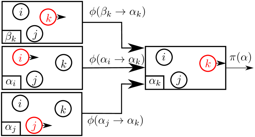
Figure 1: Probability flow diagram for three particles. The flow into any configuration has to be equal to the outflow to satisfy (maximal) global balance. Greek letters describe physical configurations and Latin letters denote lifting variables, i.e., moving particles.

Drawing on the lifting framework [19], maximal global balance is enforced by extending the physical configurations $\alpha$ by a lifting variable $i$, which sets the particle for the next move, to configurations $\alpha_{i}$ (Greek letters $\alpha,\beta,...$ describe the physical configuration, latin letters $i,j,...$ the moving particle along the direction ${\vect{e}_{\Delta}}$). We consider infinitesimal moves by vectors $\text{d}\vect{r}_{i}=\text{d}w{\vect{e}_{\Delta}}$, first along a fixed unit vector direction ${\vect{e}_{\Delta}}$. In the next move from the extended configuration $\alpha_{i}$ particle $i$ is moved by $\text{d}\vect{r}_{i}$ resulting in a new configuration $\beta_{i}$. According to the factorized Metropolis rule (2), the physical move $\alpha_{i}\!\rightarrow\!\beta_{i}$ is then either accepted by all factors $M$ (the physical configuration $\alpha$ is updated to $\beta$ and the next proposed move is again an update of particle $i$ along ${\vect{e}_{\Delta}}$) or rejected by a single factor $M$. In the latter case, a lifting move takes place, where the lifting variable $i$ changes to another particle $k$ of the set $M$ resulting in a rejection-free algorithm. We denote this lifting flow caused by the factor $M$ by $\phi_{M}(\alpha_{i}\!\rightarrow\!\alpha_{k})$.

To obey global balance (1), lifting and physical flows into a configuration $\alpha_{k}$ must add up to its Boltzmann weight $\pi(\alpha)$ as illustrated in fig. 1,

$$\phi(\beta_{k}\rightarrow\alpha_{k})+\sum_{M,k\in M}\sum_{i\in M,i\neq k}\phi_{M}(\alpha_{i}\rightarrow\alpha_{k})=\pi(\alpha)$$ (4)

(for moves with fixed vectors $\text{d}w{\vect{e}_{\Delta}}$ only one configuration $\beta_{k}$ contributes in the sum in (1)). Owing to detailed balance of the factorized Metropolis filter (2), the physical flow $\phi(\beta_{k}\!\rightarrow\!\alpha_{k})$ can be rewritten as

$$\phi(\beta_{k}\rightarrow\alpha_{k}) =\pi(\beta)p^{\text{fact}}(\beta_{k}\rightarrow\alpha_{k})=\pi(\alpha)p^{\text{fact}}(\alpha_{k}\rightarrow\beta_{k})$$

$$=\pi(\alpha)\left(1-\sum_{M,k\in M}[-\text{d}E_{k,M}]^{+}\right),$$ (5)

where $+\text{d}E_{k,M}$ is the energy change of the set $M$ for a move of a particle $k\in M$ along ${\vect{e}_{\Delta}}$ for a configurational change $\beta\!\rightarrow\!\alpha$ and $-\text{d}E_{k,M}$ the energy change for the reverse move of particle $k$. The lifting flow $\phi(\alpha_{i}\!\rightarrow\!\alpha_{k})$ must compensate for the probability of rejection in (5) to fulfill global balance (4) without rejections. We define the lifting probability $p^{\text{lift}}_{M}(\alpha_{i}\!\rightarrow\!\alpha_{k})$ from particle $i$ to $k$ within a factor $M$ by the decomposition

$$\phi_{M}(\alpha_{i}\rightarrow\alpha_{k})=\pi(\alpha)p^{\text{lift}}_{M}(\alpha_{i}\rightarrow\alpha_{k}).$$

For infinitesimal displacements only a single factor $M$ causes the rejection, i.e., only the term from the rejection causing factor $M$ contributes in the sum over lifting flows in the global balance (4) (for a more detailed discussion see ref. 16). Therefore, it suffices to consider this specific rejection causing factor $M$ for global balance in the following, so that global balance (4) is equivalent to

$$\sum_{i\in M,i\neq k}p^{\text{lift}}_{M}(\alpha_{i}\rightarrow\alpha_{k})=[-\text{d}E_{k,M}]^{+}.$$ (6)

For pairwise interactions, see ref. [11], each rejection is caused by a single interacting particle and the factors $M$ in (6) are pairs. Due to translational invariance, the resulting lifting probabilities are

$$p^{\text{lift}}_{M}(\alpha_{i}\rightarrow\alpha_{k})=[-\text{d}E_{k,i}]^{+}=[\text{d}E_{i,k}]^{+}$$ (7)

(with $\text{d}E_{i,k}\equiv\text{d}E_{i,M}$). They give rise to lifting flows, which exactly compensate for rejections in (5). Maximal global balance is fulfilled: There are no rejections on the extended configuration space and no backwards moves on the physical space. Between two lifting moves, the particle $i$ is moved by a finite displacement $\Delta w$, until a particle $k$ rejects the move and is moved in the same direction.

If the interaction is a many-body interaction, the lifting probability (7) is not correct anymore and has to be adapted. The translational invariance does not yield a symmetry between only two particles anymore but between all particles in an interacting set $M$. Moving all particles $i\in M$ by the same $\text{d}\vect{r}_{i}=\text{d}w{\vect{e}_{\Delta}}$ leaves the energy $E_{M}$ invariant,

$$\sum_{i\in M}\text{d}E_{i,M} =0.$$ (8)

In the following, we will discuss how to implement a maximal global-balance scheme for many-body interactions, as illustrated in fig. 1. First, we decompose the overall lifting probability $p^{\text{lift}}_{M}(\alpha_{i}\to\alpha_{k})$ into the trial probability to propose a lifting move from $i$ to any particle of a factor $M$ containing $i$ and $k$, $p^{\text{lift}}_{M}(\alpha_{i}\to\alpha_{M})$, and into the conditional probability $\lambda_{ik}$ to actually lift from $i$ to $k$, so that $p^{\text{lift}}_{M}(\alpha_{i}\to\alpha_{k})=p^{\text{lift}}_{M}(\alpha_{i}\to\alpha_{M})\lambda_{ik}$. In order to make the algorithm rejection-free, the trial probability has to exactly compensate the rejection probability $[\text{d}E_{i,M}]^{+}$ for the rejection-causing factor $M$ containing $i$ from (3),

$$p^{\text{lift}}_{M}(\alpha_{i}\to\alpha_{M})=[\text{d}E_{i,M}]^{+},$$

and the conditional probabilities have to be normalized: $\sum_{k\in M}\lambda_{ik}=1$.

The global balance conditions (6) become

$$\sum_{i\in M}[\text{d}E_{i,M}]^{+}\lambda_{ik}=[-\text{d}E_{k,M}]^{+}.$$ (9)

Lifting from particle $i$ to $k$, i.e., $\lambda_{ik}>0$ requires $\text{d}E_{i,M}>0$ in order to trigger lifting by rejection and $\text{d}E_{k,M}<0$ according to global balance (6). This also enforces maximal global balance as only lifting moves from $i$ to $k$ are proposed. Let us consider a set $M$ of $\mathcal{N}$ interacting particles with $\mathcal{N}_{-}$ of them having $\text{d}E_{k,M}<0$ (i.e., an update along ${\vect{e}_{\Delta}}$ leads to a decrease in energy) and $\mathcal{N}-\mathcal{N}_{-}$ having $\text{d}E_{k,M}>0$ (i.e., an update along ${\vect{e}_{\Delta}}$ leads to an increase in energy), for which we have to determine the set of $(\mathcal{N}-\mathcal{N}_{-})\mathcal{N}_{-}$ non-zero lifting probabilities $\lambda_{ik}$. The normalization $\sum_{k\in M\backslash\{i\}}\lambda_{ik}=1$ gives $(\mathcal{N}-\mathcal{N}_{-})$ conditions. Global balance (9) gives $\mathcal{N}_{-}-1$ independent conditions (summing over $k$ leads to $\sum_{i\in M}[\text{d}E_{i,M}]^{+}=\sum_{k\in M}[-\text{d}E_{k,M}]^{+}$, which is always true because of translational invariance (8)). We thus have $\mathcal{N}-1$ independent conditions on $(\mathcal{N}-\mathcal{N}_{-})\mathcal{N}_{-}$ non-zero $\lambda_{ik}$. We can conclude that for $\mathcal{N}=2,3$ these conditions are sufficient to obtain a unique set of $\lambda_{ik}$, whereas the choice of the probabilities $\lambda_{ik}$ is not unique for $\mathcal{N}\geq 4$.

For $\mathcal{N}=2$ with two interacting particles $i$ and $k$, we simply have $\lambda_{ik}=1$, such that the EC algorithm for pairwise interactions [11] is recovered. For $\mathcal{N}=3$, i.e., three-particle interactions global balance (9) and normalization uniquely determine the $\lambda_{ik}$ for the set $M=\{i,j,k\}$. If $\text{d}E_{i,jk}>0$ (with $\text{d}E_{i,jk}\equiv\text{d}E_{i,M}$) and with translational invariance (8), we have to distinguish three possible cases of signs of the energy changes $\text{d}E_{j,ik}$ and $\text{d}E_{k,ij}$:

$$\begin{aligned} \text{d}E_{j,ik}&\!>\!0,~{}~{}\text{d}E_{k,ij}\!<\!0:&&\lambda_{ij}=0,~{}\lambda_{ik}=1\\ \text{d}E_{j,ik}&\!<\!0,~{}~{}\text{d}E_{k,ij}\!>\!0:&&\lambda_{ij}=1,~{}\lambda_{ik}=0\\ \text{d}E_{j,ik}&\!<\!0,~{}~{}\text{d}E_{k,ij}\!<\!0:&&\lambda_{ij}={[-\text{d}E_{j,ik}]^{+}}/{[\text{d}E_{i,jk}]^{+}},\\ &&&\lambda_{ik}={[-\text{d}E_{k,ij}]^{+}}/{[\text{d}E_{i,jk}]^{+}}.\end{aligned}$$ (10)

For $\mathcal{N}\geq 4$, the choice of $\lambda_{ik}$ is not unique but there is a particularly simple choice, which we obtain with the additional conditions $\lambda_{ik}=\lambda_{jk}$ for all $i,j\in M$. Together with the global balance condition (9), we obtain

$$\lambda_{ik}=\frac{[-\text{d}E_{k,M}]^{+}}{\sum_{l\in M}[\text{d}E_{l,M}]^{+}}=\frac{[-\text{d}E_{k,M}]^{+}}{\sum_{l\in M\backslash\{k\}}[\text{d}E_{l,M}]^{+}}.$$ (11)

Owing to translational invariance, the normalization $\sum_{k\in M}\lambda_{ik}=1$ holds, because the translational symmetry (8) leads to $\sum_{k\in M}[-\text{d}E_{k,M}]^{+}=\sum_{l\in M}[\text{d}E_{l,M}]^{+}$.

Eq. (11) is a Glauber-like lifting rule as the lifting probability only depends on the energy change $[-\text{d}E_{k,M}]^{+}$ of the final particle $k$. For the case $\mathcal{N}=3$, the lifting rule (11) is also equivalent to a Metropolis-like representation $\lambda_{ik}=\min\left(1,[-\text{d}E_{k,ij}]^{+}/[\text{d}E_{i,jk}]^{+}\right)$.

The expression of the conditional probabilities is our main result: eq. (11) gives the rule to implement a maximal global-balance and rejection-free scheme for $\mathcal{N}$-particle interactions provided the forces onto all $\mathcal{N}$ particles are known, as the infinitesimal energy changes $\text{d}E$ correspond to the ${\vect{e}_{\Delta}}$-component of the forces on the particles. For the scheme (11), the conditional lifting probabilities $\lambda_{ik}$ depend on the MC-move direction ${\vect{e}_{\Delta}}$ and the forces onto the final particle $k$.

As for the EC algorithm for pairwise interactions, ergodicity on all directions ${\vect{e}_{\Delta}}$ is achieved by setting a finite total displacement $\ell$, [14, 11]. Once all the finite displacements $\Delta w$ between successive lifting events sum up to $\ell$, the lifting variable $i$ and the direction ${\vect{e}_{\Delta}}$ are resampled. This sequence is called an event chain, EC, and $\ell$ the length of the EC.

In practice, implementing infinitesimal moves leads to an infinite number of physical moves per unit of time. An EC move starts with a randomly chosen particle $i$ and a random direction $\vect{e}_{\Delta}$. An event-driven approach is used to compute directly the next lifting event. The maximal displacement length $w_{M}$ for all many-particle interactions between any set $M$ of $\mathcal{N}$ particles containing $i$ are calculated by solving

$$\int_{0}^{w_{M}}[\text{d}E_{i,M}(\tilde{w})]^{+}=-\ln u_{M}=\Delta E^{*}_{u_{M}},$$ (12)

with $u_{M}$ being a random number uniformly distributed in $(0,1]$ and drawn for each set $M$ such that the positive increment of energy $\Delta E^{*}_{u_{M}}$ is drawn from an exponential distribution [14]. The particle is moved by the smallest $w=\min_{M}[w_{M}]$ selecting out one particular set of $\mathcal{N}$ interacting particles for the lifting. Afterwards, the conditional lifting probabilities $\lambda_{ij}$ for this set are calculated, and the EC is lifted to the next moving particle accordingly. The computation of $\mathcal{N}-1$ lifting probabilities is not the performance-limiting step because the number of $\mathcal{N}$-particle tuples $M$, for which $w_{M}$ has to be calculated, is typically much larger. Moving and lifting are repeated until the EC length $\ell$ is reached.

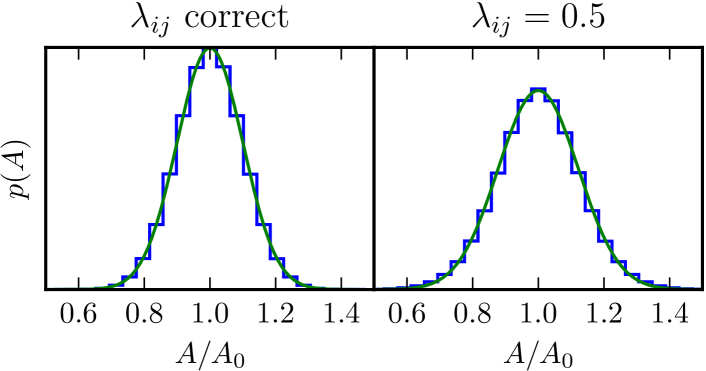
Figure 2: Histogram of measured areas with Gaussian fits. On the left we used the correct lifting ratios calculated by (10), while, on the right side, we use the choice $\lambda_{ij}=0.5$. The systems were sampled with $KA_{0}^{2}=100$ such that the theoretical prediction (14) is $\sigma_{A}=0.1\,A_{0}$ for the Gaussian distribution. We find $\sigma=(0.10068\pm 0.0003)\,{A_{0}}$ for the correct solution but $\sigma=(0.1222\pm 0.0004)\,A_{0}$ for $\lambda_{ij}=0.5$.

For applications, the determination of the displacement $w_{M}$ is often one of the main technical difficulties. As discussed in ref. [11], it is often advantageous to further decompose the interaction into several parts, e.g., $E_{M}=E_{a,M}+E_{b,M}+...$. Then, we treat each part as an independent factor in (2) and determine for each part all maximal displacement lengths $w_{a,M}$, $w_{b,M}$,… . The smallest $w=\min_{\{a,M\}}[w_{a,M}]$ gives the maximal displacement length and the conditional lifting probabilities $\lambda_{ij}$ are calculated for the set of particles $M$ and the part of the interaction $a$ minimizing $w$.

In the following sections, we validate our EC algorithm by applying it to three different systems with three-particle interactions.

3 Triangle interaction

As a first validation we investigate a simple test system of three particles in two dimensions. The three particles form a triangle of area $A$, and we define a genuine three-particle interaction by $E=\frac{K}{2}(A-A_{0})^{2}$, where $A_{0}$ is a preferred triangle area and $K$ is a coupling constant. The area can be written as $A=\frac{1}{2}|\vect{r}_{ij}\times\vect{r}_{ik}|$.

In order to calculate the maximal displacement length from eq. (12), we need to analyze the energy change $E(w)$ when moving particle $i$ along $\Delta\vect{r}_{i}=w\vect{e}_{\Delta}$ for extrema. We find three zeros of $\text{d}E(w)$,

$$w_{01}=-\frac{|\vect{r}_{ij}(0)\times\vect{r}_{ik}(0)|}{({\vect{e}_{\Delta}}\times\vect{r}_{jk})_{z}},~{}w_{02,03}=\frac{\pm 2A_{0}}{({\vect{e}_{\Delta}}\times\vect{r}_{jk})_{z}}+w_{01}.$$

At $w_{01}$ the area is zero, i.e., all three particles are on a line, while $w_{02,03}$ are points where $A=A_{0}$. Solving (12) gives the maximal displacement length

$$w=-w_{02,03}\pm\left({\left(w_{02,03}\right)^{2}+{8\Delta E}/{K|{\vect{e}_{\Delta}}\times\vect{r}_{jk}|^{2}}}\right)^{1/2}$$ (13)

where we use $w_{02}$ if $(\vect{r}_{ij}(0)\times\vect{r}_{ik}(0))_{z}<0$ and $w_{03}$ else and pick the smallest positive $w$. The lifting ratios are calculated by using (10).

The probability distribution of the area, $p(A)$, is given by the Boltzmann distribution and should therefore be Gaussian,

$$p(A)=\frac{1}{Z}e^{-E(A)}=\sqrt{\frac{K}{2\pi}}e^{-\frac{K}{2}(A-A_{0})^{2}},$$ (14)

with mean $\langle A\rangle=A_{0}$ and a variance $\sigma_{A}^{2}=K^{-1}$. In order to validate our algorithm we measure $p(A)$ and compare with the theoretical prediction (14), see fig. 2. The correct choice of conditional lifting probabilities $\lambda_{ij}$ agrees with the theoretical prediction, whereas other choices such as $\lambda_{ij}=0.5$ give rise to clear deviations.

4 Hard needles in two dimensions

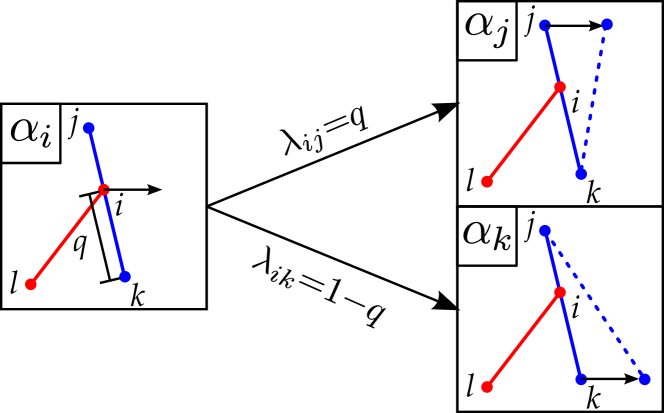
Figure 3: Lifting probabilities $\lambda_{ij}$ and $\lambda_{ik}$ when a moving end point $i$ hits a fixed needle $jk$ (see eq.(16)).

We now consider a system of hard extensible needles in two dimensions (2D), which are described in terms of the coordinates of their end points; the end point ensemble thus constitutes a many-particle system that is treated with the EC algorithm. Each needle $ij$ is extensible with a pair energy $E_{el}=\frac{1}{2}K(|\vect{r}_{ij}|-L)^{2}$, where $K$ is an elastic constant and $L$ the needle rest length; we will focus on large $K$ to ensure almost fixed length $L$. The repulsive hard core interaction of the lines connecting the end points is modeled as three-particle interaction between each end point $i$ and the line $jk$ connecting the two end points $j$ and $k$ of any second needle, see fig. 3. In order to describe this interaction we introduce the parallel component $r_{ki,||}=\vect{r}_{ki}\cdot\vect{e}_{jk}$ of $\vect{r}_{ki}$ from $k$ to $i$ (using the unit vector $\vect{e}_{jk}\equiv\vect{r}_{jk}/|\vect{r}_{jk}|$ parallel to the needle $jk$) and the perpendicular distance $d_{i,jk}=|\vect{r}_{ki}-\vect{e}_{jk}r_{ki,||}|$ of point $i$ to the needle $jk$.

The Boltzmann weight of the hard needle interaction is zero if end point $i$ touches the needle $jk$ and one otherwise and can be written as

$$\pi_{i,jk}=1-(1-\Theta(d_{i,jk}))\Theta_{L}(r_{ki,||}),$$ (15)

with the Heaviside function $\Theta(x)$ ($=0$ for $x=0$ and $=1$ for $x>0$) and another indicator function $\Theta_{L}(x)$ with $\Theta_{L}(x)=1$ for $0<x<L$ and $\Theta_{L}(x)=0$ otherwise.

Lifting occurs whenever an end point hits another needle. This can happen either because the moving end point hits a fixed needle or the moving needle (belonging to the moving end point) hits an end point of a fixed needle. If an end point $i$ hits the needle $jk$ the EC algorithm needs to decide whether to lift to point $j$ or $k$, which gives the next end point to displace, see fig. 3. For this decision we need to calculate the conditional lifting probabilities $\lambda_{ij}$ and $\lambda_{ik}$, given by (10). For the hard needle interaction, we use the derivative of the Boltzmann weights $\text{d}E_{i,jk}=-\text{d}\pi_{i,jk}/\pi(\alpha)$ (see eq. (3)) with

$$\frac{-\text{d}\pi_{i,jk}}{\text{d}w}=-(\nabla_{\vect{r}_{i}}d_{i,jk}\cdot{\vect{e}_{\Delta}})\delta(d_{i,jk})\Theta_{L}(r_{ki,||})$$

$$+(\nabla_{\vect{r}_{i}}r_{ki,||}\cdot{\vect{e}_{\Delta}})(\delta(r_{ki,||})-\delta(L-r_{ki,||}))(1-\Theta(d_{i,jk})).$$

The second term is non-zero only if the needle point $i$ exactly hits one of the ends of the needle $jk$ and can therefore be neglected for infinitely thin needles. Using this in eq. (10) we find

$$\lambda_{ik}=\frac{\left[\nabla_{\vect{r}_{k}}d_{i,jk}\cdot{\vect{e}_{\Delta}}\right]^{+}}{\left[-\nabla_{\vect{r}_{i}}d_{i,jk}\cdot{\vect{e}_{\Delta}}\right]^{+}+\left[-\nabla_{\vect{r}_{j}}d_{i,jk}\cdot{\vect{e}_{\Delta}}\right]^{+}}$$ (16)

with $\nabla_{\vect{r}_{k}}d_{i,jk}\cdot{\vect{e}_{\Delta}}=(\hat{\vect{r}}_{ik,\perp}\cdot{\vect{e}_{\Delta}})|r_{ik,||}|/|r_{jk}|$ and $\nabla_{\vect{r}_{i}}d_{i,jk}\cdot{\vect{e}_{\Delta}}=-(\hat{\vect{r}}_{ik,\perp}\cdot{\vect{e}_{\Delta}})$.

When the moving end point $i$ hits the needle $jk$, this simplifies to simple length ratios $\lambda_{ij}=|r_{ik,||}|/|r_{jk}|\equiv q$ and $\lambda_{ik}=|r_{ij}|/|r_{jk}|=1-q$, where $|r_{jk}|\approx L$. When, vice versa, point $k$ is moving and an end point $i$ is hit by the moving needle $jk$, it gives $\lambda_{ki}=1$ and $\lambda_{kj}=0$, i.e., the EC then transfers to $k$ with certainty. The elastic pair energy $E_{el}$ is treated independently as an additional simple pairwise interaction using eq.(7).

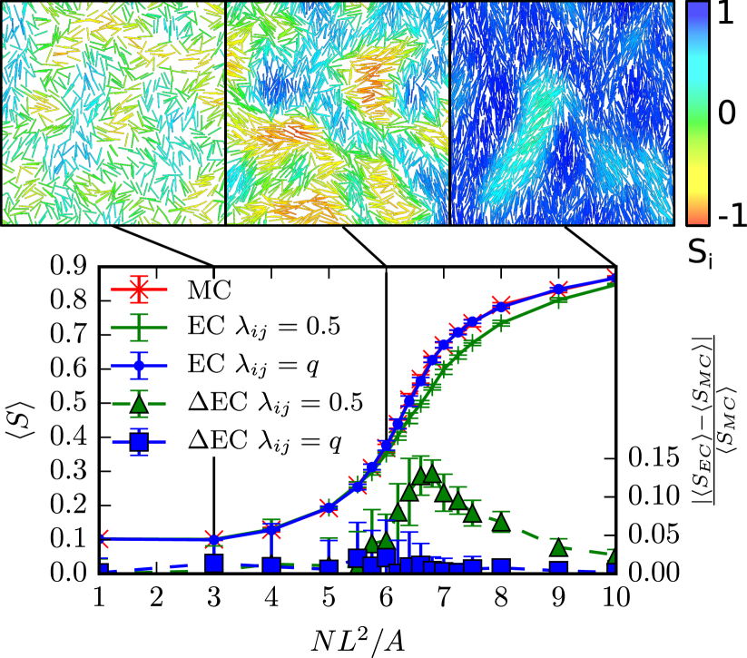
Figure 4: Nematic order parameter $\langle S\rangle$ (left axis) and relative deviation of EC results to local MC (right axis) as a function of the number of needles $N$ per area $A$ for a 2D system of needles with $K=100/L^{2}$ with periodic boundaries ($A=10L\times 10L$) (left axis). The EC algorithm with $\lambda_{ij}=q=1-\lambda_{ik}$, see eq. (16), agrees numerically with local MC, whereas a naive choice $\lambda_{ij}=\lambda_{ik}=0.5$ significantly deviates. Upper row: Simulation snapshots color-coded for the local order parameter $S_{i}=2\cos^{2}\theta_{i}-1$ around needle $i$.

In order to validate our algorithm we measure the nematic order parameter of the 2D hard needle system $S=2\langle\cos^{2}\theta\rangle-1$, with $\theta$ being the angle between the needle orientation and the director as a function of needle density. In fig. 4, we compare local MC simulations with rejections and two versions of the EC algorithm. In one version we naively take $\lambda_{ij}=\lambda_{ik}=1/2$, the other version is the proper algorithm using (16)

Measuring the autocorrelation time for the order parameter $\langle S\rangle$ we find speed-up factors of $3-4$ in CPU time for the EC algorithm in comparison to the local MC algorithm (measured at $NL^{2}/A=6$). This algorithm can also be used in polymer simulation where the polymers are modeled as chains of hard needles as alternative to existing polymer EC algorithms [18].

5 Semiflexible polymer

As a third application we simulate a free semiflexible harmonic chain with bending rigidity $\kappa$ composed of $N$ beads and elastic bonds of mean length $b=1$ [20], i.e. mean contour length $L=Nb$, in three dimensions. The bending energy is

$$E_{b}=\kappa\sum_{i=1}^{N-2}\left(1-\frac{\vect{t}_{i}\cdot\vect{t}_{i+1}}{|\vect{t}_{i}||\vect{t}_{i+1}|}\right)=\kappa\sum_{i=1}^{N-2}\big{(}1-\cos(\theta_{i+1})\big{)}$$ (17)

with tangential vectors $\vect{t}_{i}=\vect{r}_{i+1}-\vect{r}_{i}$ and tangential angles $\theta_{i}$ at bead $i$. Moving bead $i$ changes three terms in (17) since $\vect{t}_{i-1}$, $\vect{t}_{i}$ and $\vect{t}_{i+1}$ are functions of $\vect{r}_{i}$ and three angles change (see fig. 5). Each angle is a function of three particle positions, making the bending energy a three-particle interaction. MC algorithms working on bead positions rather than angles are important for the simulation of many-polymer systems or polymers in external potentials, where interactions are position-dependent.

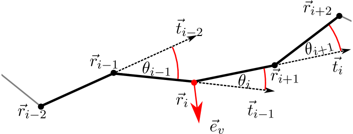
Figure 5: Moving bead $i$ in a semiflexibe polymer changes three angles.

We first determine the maximal displacement length for a displacement $\Delta\vect{r}_{i}=w\vect{e}_{\Delta}$ of bead $i$. In the following, $x$ is the remaining total displacement length of the EC, i.e. $w\leq x$.

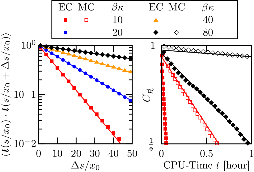
Figure 6: Left: Tangent correlation function and expected exponential decay (dashed) for different values of $\kappa$ and $N=240$ beads. Right: Autocorrelation $C_{\vect{R}}(\Delta t)$ of the end-to-end-vector as a function of CPU time $t$ (on a $3.7$GHz Intel Xeon CPU) for local MC and the new EC algorithm. Lines are exponential fits $\sim e^{-t/\tau}$.

For an outer angle $\theta_{i-1}$ the energy change is

$$\text{d}E_{i,\theta_{i-1}}(w) =-\frac{\kappa}{|\vect{t}_{i-2}||\vect{t}_{i-1}+w\vect{e}_{\Delta}|^{3}}(a+wb)\text{d}w,$$

$$a \equiv\big{(}\vect{t}_{i-1}^{2}(\vect{t}_{i-2}\cdot\vect{e}_{\Delta})-(\vect{t}_{i-1}\cdot\vect{t}_{i-2})(\vect{t}_{i-1}\cdot\vect{e}_{\Delta})\big{)}$$

$$b \equiv\big{(}(\vect{t}_{i-1}\cdot\vect{e}_{\Delta})(\vect{t}_{i-2}\cdot\vect{e}_{\Delta})-(\vect{t}_{i-1}\cdot\vect{t}_{i-2})\big{)},$$

which gives an extremum of the energy $E_{i,\theta_{i-1}}(w)$ at $w_{0}=-a/b$. For the calculation of the maximal displacement length we calculate $w_{0}$ and the sign of $\text{d}E_{i,\theta_{i-1}}(w=0)$. If $\text{d}E_{i,\theta_{i-1}}(w=0)<0$, $E_{i,\theta_{i-1}}(w)$ is decreasing. If $w_{0}<0$ the bead can move until $w=x$ is reached (and the EC terminates). If $w_{0}>0$ there is an energy minimum at $w_{0}$, to which the bead can move at no energy cost. We calculate the energy $E_{\text{\rm min}}$ and allow an energy increase of $\Delta E$ to $E_{\text{\rm new}}=E_{\text{\rm min}}+\Delta E$. The corresponding displacement length $w_{+}$ is calculated by solving

$$\cos{\theta_{+}}\equiv 1-\frac{E_{\text{\rm new}}}{\kappa}=\frac{\vect{t}_{i-2}\cdot(\vect{t}_{i-1}+w_{+}\vect{e}_{\Delta})}{|\vect{t}_{i-2}||\vect{t}_{i-1}+w_{+}\vect{e}_{\Delta}|},$$

which gives

$$w_{+}=-{B}/{A}\pm\sqrt{\left({B}/{A}\right)^{2}-{C}/{A}},$$ (18)

$$A \equiv(\vect{t}_{i-2})^{2}\cos^{2}(\theta_{+})-(\vect{t}_{i-2}\cdot\vect{e}_{v})^{2},$$

$$B \equiv(\vect{t}_{i-1}\cdot\vect{e}_{v})(\vect{t}_{i-2})^{2}\cos^{2}(\theta_{+})-(\vect{t}_{i-2}\cdot\vect{t}_{i-1})(\vect{t}_{i-2}\cdot\vect{e}_{v}),$$

$$C \equiv(\vect{t}_{i-1})^{2}(\vect{t}_{i-2})^{2}\cos^{2}(\theta_{+})-(\vect{t}_{i-2}\cdot\vect{t}_{i-1})^{2},$$

where we take the smallest positive solution in (18), and the maximal displacement length is $w=w_{0}+w_{+}$. If ${\text{d}E_{i,\theta_{i-1}}(w=0)>0}$, $E_{i,\theta_{i-1}}(w)$ is increasing and there is an energy minimum at $w_{0}$. Then we calculate $w_{+}$ immediately using (18) with $E_{\text{\rm new}}=E_{i,\theta_{i-1}}(0)+\Delta E$. If $w_{+}$ is smaller than the energy-maximizing $w_{0}$ or $w_{0}<0$, $w_{+}$ is the maximal displacement length. Otherwise, the move over the energy maximum at $w_{0}$ can be performed so the bead can move until $w=x$ is reached (and the EC terminates). Analogous calculations apply to $\theta_{i+1}$.

The calculation for the center angle $\theta_{i}$ is more complicated because $\text{d}E_{i,\theta_{i}}(w)$ has one or three zeros. Since the energy $E_{i,\theta_{i}}(w)$ gets maximized for $w\rightarrow\pm\infty$, $E_{i,\theta_{i}}(w)$ either has two minima and one maximum in between or only a single minimum. The algorithm now works as follows: First the zeros $z_{i}$ with $\text{d}E_{i,\theta_{i}}(z_{i})=0$ are calculated Since only zeros in the moving direction are important there can be up to three extrema on the way. These four cases are treated as follows:
0 zeros: $\text{d}E_{i,\theta_{i}}>0$ so moving costs energy. The energy cost for moving the complete remaining $x$ can be calculated. If the cost is smaller than $\Delta E$ this move is performed. Otherwise, $w$ is calculated numerically by solving $E_{i,\theta_{i}}(w)=E_{i,\theta_{i}}(0)+\Delta E$.
1 zero: $z_{1}$ is a minimum. Set $x=x-z_{1}$ and go to case no zeros as explained above.
2 zeros: The first zero $z_{1}$ is a maximum, the second one $z_{2}$ a minimum. If the maximum can be reached with the energy $\Delta E$, the available energy $\Delta E$ is reduced by the energy cost $\Delta E=\Delta E-(E_{i,\theta_{i}}(z_{2})-E_{i,\theta_{i}}(z_{1}))$. Set $x=x-z_{1}$ and continue at case 1 zero as above with $z_{1}=z_{2}-z_{1}$ If the maximum at $z_{1}$ cannot be reached, $w$ is calculated numerically on the interval $[0,z_{1}]$.
3 zeros: Then, $z_{1}$ is a minimum, which means the particle can move to $z_{1}$. Set $x=x-z_{1}$ and continue at case 2 zeros as above with $z_{1}=z_{2}-z_{1}$ and $z_{2}=z_{3}-z_{1}$.

We validate the correctness of this algorithm by measuring the tangent correlation function $\langle\vect{t}(s)\cdot\vect{t}(s+\Delta s)\rangle$, which is analytically known to decay as $e^{-\Delta s/L_{p}}$ (for $\Delta s\ll N$) with the persistence length $L_{p}=-1/\ln(1/\tanh\kappa-1/\kappa)$ [21]. As seen in fig. 6 the measured values match the analytical curve.

To measure the efficiency of the algorithm the autocorrelation of the end-to-end-vector $\vect{R}=\vect{r}_{N}-\vect{r}_{0}$ is calculated as

$$C_{\vect{R}}(\Delta t)=\frac{\langle\vect{R}(t)\cdot\vect{R}(t+\Delta t)\rangle-\langle\vect{R}\rangle^{2}}{\langle\vect{R}^{2}\rangle-\langle\vect{R}\rangle^{2}}\underset{\Delta t\gg 1}{\sim}e^{-\Delta t/\tau},$$ (19)

where the time is measured in real time to allow a comparison of the EC algorithm with the local MC method The results are shown in fig. 6. For $\beta\kappa=10$ we get $\tau_{\rm MC}\approx 0.72{\rm h}$ and $\tau_{\rm EC}=0.06{\rm h}$, which means the EC algorithm is approx. $11.3$ times faster at equilibrating a semiflexible polymer than the standard local MC method. For $\beta\kappa=80$ the EC performs even better: we get $\tau_{\rm MC}\approx 15{\rm h}$ and $\tau_{\rm EC}=1.1{\rm h}$, which gives a speed-up of approx. $14$.

6 Discussion and Conclusion

We generalized the EC algorithm to three-particle and many-particle interactions thus broadening the range of applicability of rejection-free EC algorithms considerably. For $\mathcal{N}$-particle interactions, there are $\mathcal{N}-1$ interacting particles to which the EC can lift to avoid rejections. We calculate a set of $\mathcal{N}-1$ conditional lifiting probabilities $\lambda_{ij}$ which assure maximal global balance.

We applied the generalized EC algorithm successfully to three different systems – a small system with three particles with a triangle-area-dependent interaction, hard needles in 2Ds, and a single semiflexible polymer chain with bending energy – and demonstrate in all three cases the correctness of the algorithm. For hard needles or the semiflexible polymer we obtain considerable performance gains.

In the future, the EC algorithm can be used for efficient large scale simulations of the 2D hard needle system to answer the questions as to whether nematic long-range order exists in large systems (the increase of $S$ to a large value in fig. 4 can be an artefact of finite size effects) and whether the system has a Kosterlitz-Thouless transition around $\rho\sim 7/L^{2}$ by disclination unbinding, as suggested by local MC results [22, 23]. Future work should also evaluate systematically to what extent the EC algorithm can suppress critical slowing down at the transition from isotropic to (quasi-)nematic.

With respect to polymer simulations, the algorithm will allow the entirely rejection-free simulation of large systems containing many interacting semiflexible polymers [18, 12]. In our previous work[18] hybrid EC algorithms were slower than algorithms where all interactions are handled by the EC scheme, so that we expect that the simulation of many-polymer systems with bending energies will also benefit from the $\mathcal{N}$-particle EC algorithm.

References

- [1] \NameLandau D. P. Binder K. \BookA Guide to Monte Carlo Simulations in Statistical Physics \PublCambridge University Press, Cambridge \Year2015
- [2] \NameFrenkel D. Smit B. \BookUnderstanding Molecular Simulation: From Algorithms to Applications \PublAcademic Press, San Diego \Year2002
- [3] \NameSwendsen R. Wang J. \REVIEWPhys. Rev. Lett.58198786.
- [4] \NameWolff U. \REVIEWPhys. Rev. Lett.621989361.
- [5] \NameDress C. Krauth W. \REVIEWJ. Phys. A: Math. and Gen.281995L597
- [6] \NameBuhot A. Krauth W. \REVIEWPhys. Rev. Lett.8019983787
- [7] \NameSanten L. Krauth W. \REVIEWNature4052000550
- [8] \NameLiu J. Luijten E. \REVIEWPhys. Rev. Lett.922004035504
- [9] \NameBernard E. P., Krauth W. Wilson D. B. \REVIEWPhys. Rev. E802009056704.
- [10] \NameBernard E. Krauth W. \REVIEWPhys. Rev. Lett.1072011155704
- [11] \NameMichel M., Kapfer S. C. Krauth W. \REVIEWJ. Chem. Phys.1402014054116
- [12] \NameKampmann T. A., Boltz H.-H. Kierfeld J. \REVIEWJ. Comp. Phys.2812014864-875
- [13] \NameIsobe M. Krauth W. \REVIEWJ. Chem. Phys.1432015084509
- [14] \NamePeters E. A. J. F. De With G. \REVIEWPhys Rev. E852012026703
- [15] \NameKapfer S.C. Krauth W. \REVIEWPhys. Rev. Lett.1142015035702
- [16] \NameMichel M., Mayer J. Krauth W. \REVIEWEPL112201520003
- [17] \NameNishikawa Y., Michel M.,Krauth W. Hukushima K. \REVIEWPhys. Rev. E922015063306
- [18] \NameKampmann T. A., Boltz H.-H. Kierfeld J. \REVIEWJ. Chem. Phys.1432015044105
- [19] \NameDiaconis P., Holmes, S. Neal, R.M. \REVIEWAnn. Appl. Probab.102000726
- [20] \NameKierfeld J., Niamploy O., Sa-yakanit V. Lipowsky R. \REVIEWEuro. Phys. Journal E14200417-34
- [21] \NameKleinert H. \BookPath Integrals in Quantum Mechanics, Statistics, Polymer Physics, and Financial Markets \PublWorld Scientific, Singapore \Year2006
- [22] \NameFrenkel D. Eppenga R. \REVIEWPhys Rev. A3119851776
- [23] \NameVink R.L.C. \REVIEWEur. Phys. J. B722009225