Relation between spectral changes and the presence of the lower kHz QPO in the neutron-star low-mass X-ray binary 4U 1636$-$53

Abstract

We fitted the $3-180$-keV spectrum of all the observations of the neutron-star low-mass X-ray binary 4U 1636$-$53 taken with the Rossi X-ray Timing Explorer using a model that includes a thermal Comptonisation component. We found that in the low-hard state the power-law index of this component, $\Gamma$, gradually increases as the source moves in the colour-colour diagram. When the source undergoes a transition from the hard to the soft state $\Gamma$ drops abruptly; once the source is in the soft state $\Gamma$ increases again and then decreases gradually as the source spectrum softens further. The changes in $\Gamma$, together with changes of the electron temperature, reflect changes of the optical depth in the corona. The lower kilohertz quasi-periodic oscillation (kHz QPO) in this source appears only in observations during the transition from the hard to the soft state, when the optical depth of the corona is high and changes depends strongly upon the position of the source in the colour-colour diagram. Our results are consistent with a scenario in which the lower kHz QPO reflects a global mode in the system that results from the resonance between, the disc and/or the neutron-star surface, and the Comptonising corona.

Accepted. Received; in original form

1 introduction

Energy spectra and colour-colour diagrams (CD) are often used to study neutron-star low-mass X-ray binaries (NS-LMXBs; e.g., Hasinger & van der Klis, 1989). The evolution of the energy spectrum and the tracks on the CD are thought to be driven by variations of mass accretion rate, and reflect changes in the configuration of the accretion flow (e.g., Hasinger & van der Klis, 1989; Méndez et al., 1999; Done et al., 2007). In the low-hard state the accretion rate is low, the disc is truncated at large radii (Gierliński & Done, 2002; Sanna et al., 2013; Plant et al., 2015, see however Lin et al. 2007) and the energy spectrum is dominated by a hard/Comptonised power-law component. When the source accretion rate increases, the disc truncation radius decreases and eventually reaches the last stable orbit. In the high-soft state the accretion rate is high and the energy spectrum is dominated by a soft component, possibly a combination of the accretion disc and the neutron star.

The characteristic frequencies (e.g., quasi-periodic oscillations, QPOs) in the power density spectra (PDS) of these systems also change with the source luminosity and inferred mass accretion rate (e.g., Méndez et al., 1999; Belloni et al., 2005). Kilohertz (kHz) QPOs have been detected in many NS-LMXBs (for a review see van der Klis, 2006, and references therein). The upper kHz QPO (from the pair of QPOs the one at the highest frequency) in these systems has been interpreted in terms of characteristic frequencies (e.g., the Keplerian frequency) in a geometrically thin accretion disc (Miller et al., 1998; Stella & Vietri, 1998). In this scenario, changes of the upper kHz QPO frequency reflect changes of the inner disc radius, driven by mass accretion rate. Indeed, the frequency of the upper kHz QPOs is strongly correlated with the hard colour of the source (Méndez et al., 1999; Belloni et al., 2005; Belloni et al., 2007; Sanna et al., 2012).

Several models have been proposed to explain the lower kHz QPO in these systems. Stella & Vietri (1998) suggested a Lense-Thirring precession model, in which the frequencies of the QPOs are associated with the fundamental frequencies of geodesic motion of clumps of gas around the compact object. In the relativistic resonance model (Kluzniak & Abramowicz, 2001; Lee et al., 2001; Kluźniak et al., 2004), the kHz QPOs appear at frequencies that correspond to a coupling between two oscillations modes of the accretion disc. In the beat-frequency model (Miller et al., 1998), the lower kHz QPO originates from the interaction between the spin frequency of the NS and material orbiting at the inner edge of the accretion disc. None of these models, however, have so far been able to fully explain all the properties of kHz QPOs (e.g., Jonker et al., 2002; Belloni et al., 2005; Altamirano et al., 2012).

4U 1636–53 is a NS-LMXB that shows regular state transitions with a cycle of $\sim$40 days (e.g., Belloni et al., 2007), making it an excellent source to study correlations between its spectral and timing properties. The full range of spectral states (low/hard state, high/soft state, transitional state) has been observed in this source (Belloni et al., 2007; Altamirano et al., 2008). A pair of kHz QPOs were discovered by Wijnands et al. (1997) and Zhang et al. (1997). The upper kHz QPO has been observed in different states. Its central frequency shows a clear correlation with the hard colour of the source (Belloni et al., 2007; Sanna et al., 2012). The lower kHz-QPO in 4U 1636–52 is only detected over a narrow range of hard colour values (Belloni et al., 2007; Sanna et al., 2012). The emission mechanism of the lower kHz-QPO is still unclear (e.g., Berger et al., 1996; Méndez et al., 2001; Méndez, 2006)

We analysed the broadband energy spectra of 4U 1636–53 to investigate the evolution of the different spectral and timing components as a function of the spectral state of the source. A comparison the different continuum components in the energy spectrum with the properties of the kHz QPOs at the same state may provide an important clue to understand the origin of the kHz QPOs and the evolution of the accretion flow geometry. In §2 we describe the observations, data reduction and analysis methods, and in §3 we present the results on the temporal and spectral analysis of these data. Finally, in §4 we discuss our findings and summarise our conclusions.

2 Observations and data analysis

2.1 Data reduction

We analysed the whole archival data (1576 observations) from the Rossi X-ray Timing Explorer (RXTE) Proportional Counter Array (PCA; Jahoda et al., 2006) and the High-Energy X-ray Timing Experiment (HEXTE; Rothschild et al., 1998) of the NS-LMXB 4U 1636–53. We reduced the data using the heasoft package version 6.13. We extracted PCA spectra from the Proportional Counter Unit number 2 (PCU-2) only, since this was the best-calibrated detector and the only one which was always on in all the observations. To extract the spectra of the source we first examined the light curves to identify and remove X-ray bursts from the data. For the HEXTE data we generated the spectra using cluster B only, since after January 2006 cluster A stopped rocking and could no longer measure the background. For each observation we extracted one PCA and HEXTE X-ray spectrum, respectively. The PCA and HEXTE background spectra were extracted using the standard RXTE tools pcabackest and hxtback, respectively. We built instrument response files for the PCA and HEXTE data using pcarsp and hxtrsp, respectively.

2.2 Timing analysis

For each observation we computed Fourier power density spectra (PDS) in the $2-60$ keV band every 16 s from event-mode data. For this we binned the light curves to 1/4096 s, corresponding to a Nyquist frequency of 2048 Hz. Before computing the Fourier transform we removed detector dropouts, but we did not subtract the background or applied any dead-time correction before calculating the PDS. Finally we calculated an average PDS per observation normalised as in Leahy et al. (1983). We finally used the procedures described in Sanna et al. (2012) to detect and fit the QPOs in each PDS. We detected kHz QPOs in 581 out of 1576 observations. We detected the lower kHz QPO in 403 out of those 583 observations.

2.3 Spectral analysis

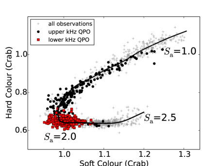
Figure 1: The colour-colour diagram of 4U 1636–53. Each point in the plot corresponds to a single RXTE observation. The filled circles (black) and the filled squares (red) represent the observations with upper and lower kHz QPOs, respectively. The gray crosses represent observations in which no kHz QPO was detected. The position of the source on the diagram is parametrized by the length of the black solid curve $S_{\rm a}$

We used the Standard-2 data (16-s time-resolution and 129 channels covering the full $2-60$ keV PCA band) to calculate X-ray colours of the source (see Zhang et al., 2009, for details). We defined hard and soft colours as the $9.7-16.0/6.0-9.7$ keV and $3.5-6.0/2.0-3.5$ keV count rate ratios, respectively. We show the CD of all observations of 4U 1636$-$53 in Figure 1, with one point per RXTE observation. In that figure we parameterised the position of the source in the CD by the length of the solid curve $S_{\rm a}$ (see, e.g. Méndez et al., 1999), fixing the values of $S_{\rm a}=1$ and $S_{\rm a}=2$ at the top-right and the bottom-left vertex of the CD, respectively.

For the spectral analysis of 4U 1636–53, we used the package xspec v12.7 (Arnaud, 1996). We fitted the PCA and HEXTE spectra simultaneously in the 3.0$-$25.0 and 25.0$-$180.0 keV range, respectively. We included the effect of interstellar absorption using the component phabs with cross-sections of Balucinska-Church & McCammon (1992) and solar abundances from Anders & Grevesse (1989), and we fixed the column density to $N_{\rm H}=3.1\times 10^{21}$ cm^-2 (Sanna et al., 2013). We added a multiplicative factor to the model to account for calibration uncertainties between the PCA and HEXTE. We set this factor to unity for the PCA and left it free for the HEXTE spectra.

Many models have been proposed to fit the spectra of accreting NS-LMXBs in the past (e.g. Barret, 2001; Lin et al., 2007). Most models include at least two components: a soft thermal component that represents the emission from the NS surface (or boundary layer) and the accretion disc, and a hard Comptonised component that represents the emission from a corona of hot electrons.

In the spectral fitting of 4U 1636–53 we used the same continuum model as in Sanna et al. (2013), who fit XMM-Newton data down to 0.8 keV. We used a multi-colour disc blackbody (diskbb in xspec) to fit the thermal emission from the disc, a single-temperature black body (BB, bbodyrad in xspec) to fit the thermal emission from the NS surface (or boundary layer), and a Comptonisation model, nthcomp, to fit the Comptonised component (Zdziarski et al., 1996; Życki et al., 1999).

The parameters of bbodyrad and diskbb are the blackbody temperature, $kT_{\rm bb}$, the temperature at the inner disc radius, $kT_{\rm dbb}$, and their normalisations, respectively. The parameters of nthcomp are the asymptotic power-law photon index, $\Gamma$, the electron temperature of the corona, $kT_{\rm e}$, the seed photon temperature, $kT_{\rm seed}$, and the normalisation. The seed photons can be from either the NS surface and boundary layer or the accretion disc. Sanna et al. (2013) analysed the spectra of six observations of 4U 1636–53 taken with XMM-Newton and RXTE simultaneously. They tried both the bbodyrad or the diskbb component as the source of seed photons for nthcomp, and concluded that diskbb was the best option. Therefore, in this work we chose diskbb as the source of the soft seed photons and we linked the seed photons temperature in nthcomp to the temperature of the diskbb component. In the fits, the value of $\Gamma$ was constrained to be larger or equal to 1.1 (Gierliński & Done, 2002; Sanna et al., 2013) and the value of $kT_{\rm e}$ was restricted to be larger or equal to 2.5 keV (Gierliński & Done, 2002; Lyu et al., 2014)

From the initial fits, there were always relatively broad residuals between 6 and 7 keV in the RXTE/PCA spectra. These residuals likely reflect the presence of an iron line in the data. The iron line has also been confirmed with XMM-Newton and Suzaku observations (Sanna et al., 2013; Lyu et al., 2014). We then added a Gaussian component with a variable width to the spectrum to fit this line. Due to the low spectral resolution of the PCA ($\sim$1 keV at $6$ keV), we can not constrain the central value of the line very well. So we fixed the line at 6.5 keV in all our fittings.

Fitting simultaneously data taken from XMM-Newton and RXTE, Sanna et al. (2013) found that the temperature of bbodyrad was $kT_{\rm bb}\sim 1.7$ keV, and remained more or less constant as the source moved across the CD. They also found that the temperature at the inner edge of the accretion disc ranged from $\sim$0.2 keV to $\sim$0.8 keV when the source moved from the low/hard to the high/soft state. Since the PCA only extends down to 3 keV, $kT_{\rm bb}$ and $kT_{\rm dbb}$ are difficult to constrain simultaneously. Therefore, we initially left $kT_{\rm dbb}$ free and, following the results of Sanna et al. (2013), we fixed $kT_{bb}$ to 1.7 keV. We then repeated the analysis fixing $kT_{\rm bb}$ to each of these values: 1.5, 1.6, 1.8, 1.9 and 2.0 keV.

From the previous analysis we found that $kT_{\rm dbb}$, linked to $kT_{\rm seed}$ in nthcomp, was not well constrained during the fits. We therefore interpolated the value of $kT_{\rm dbb}$ along the CD using the XMM-Newton–RXTE spectra fitting results in Sanna et al. (2013). We divided the data into 7 groups based on their $S_{\rm a}$ values: $<1.2$, $1.2-1.4$, $1.4-1.6$, $1.6-1.8$, $1.8-2.0$, $2.0-2.2$ and $>2.2$. In each group we fixed $kT_{\rm dbb}$ to the interpolated temperatures for $S_{\rm a}$ equal to 1.1, 1.3, 1.5, 1.7, 1.9, 2.1, and 2.35, respectively. In this case we left $kT_{\rm bb}$ free during the fits.

3 Results

3.1 X-ray spectral evolution

In Figure 2 we show the asymptotic power-law photon index, $\Gamma$, as a function of $S_{\rm a}$ in 4U 1636–53. The value of $kT_{\rm bb}$ indicated in each panel was fixed during the fittings. When the source evolves from the hard spectral state to the transitional state in the CD, the value of $S_{\rm a}$ increases from 1.0 to 2.0, $\Gamma$ increases from 1.8 to 2.2 and the source spectrum becomes soft. As the source moves through the vertex in the CD, $S_{\rm a}\sim 2.1$, $\Gamma$ drops sharply to $\sim 1.6$, and covers the range from $\sim 1.6$ to $\sim 2.2$. When the source moves out of the vertex to the bottom right part of the CD $\Gamma$ increases to $\sim 2.2$, and finally decreases back to $1.8-2.0$ as $S_{\rm a}$ increases to $\sim$2.5. It is clear from all panels that $\Gamma$ shows a significant drop at $S_{\rm a}\sim 2.1$, regardless of the value we choose for $kT_{\rm bb}$. Moreover, at low $S_{\rm a}$ values ($S_{\rm a}<2.0$), $\Gamma$ shows a larger spread for low $kT_{\rm bb}$ values. This likely indicates that the lower blackbody temperature (e.g. $<1.6$ keV) yields comparatively less well-constrained fits of the thermal Comptonisation model in 4U 1636$-$53.

The upper left panel of Figure 3 shows $\Gamma$ as a function of $S_{\rm a}$ when we used the interpolated values of $kT_{\rm dbb}$ and left $kT_{\rm bb}$ free. The trend in this Figure is similar to those in Figure 2. In the upper right panel Figure 3 we show the electron temperature, $kT_{\rm e}$, as a function of $S_{\rm a}$. As the source evolves from the hard to the transitional, and then to the soft spectral state $kT_{\rm e}$ first decreases from $\sim 30$ keV to $\sim 3$ keV and then stays more or less constant.

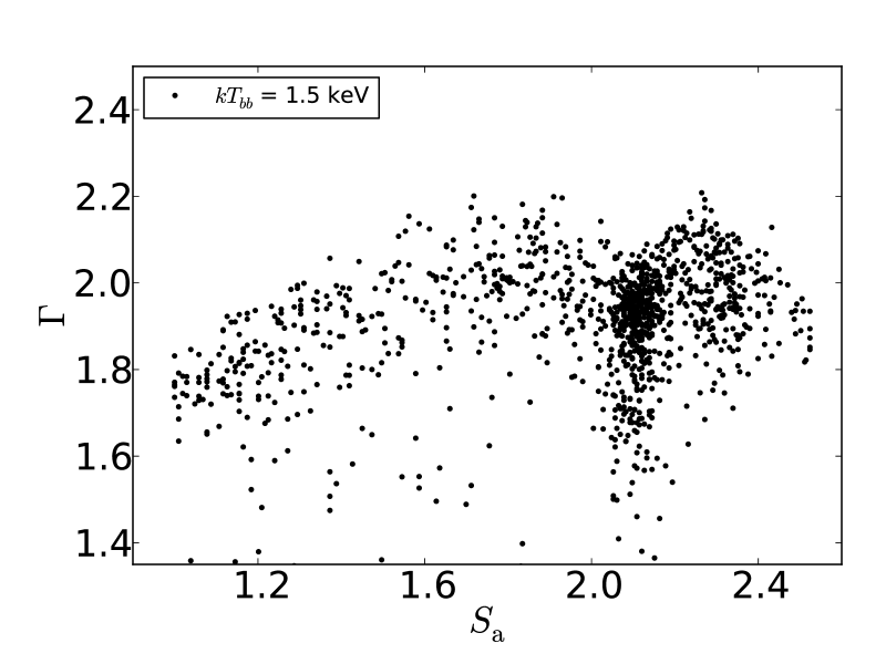
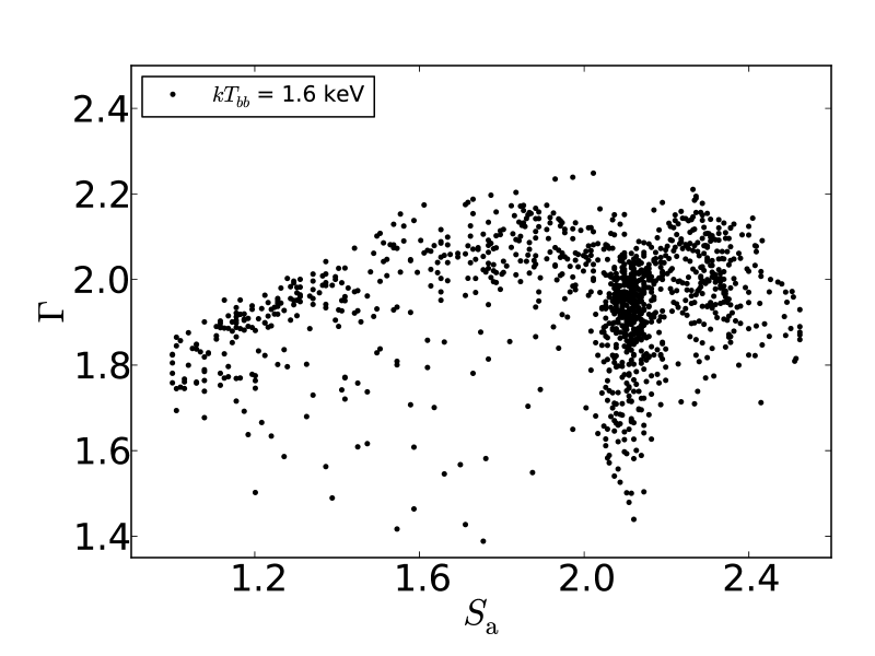
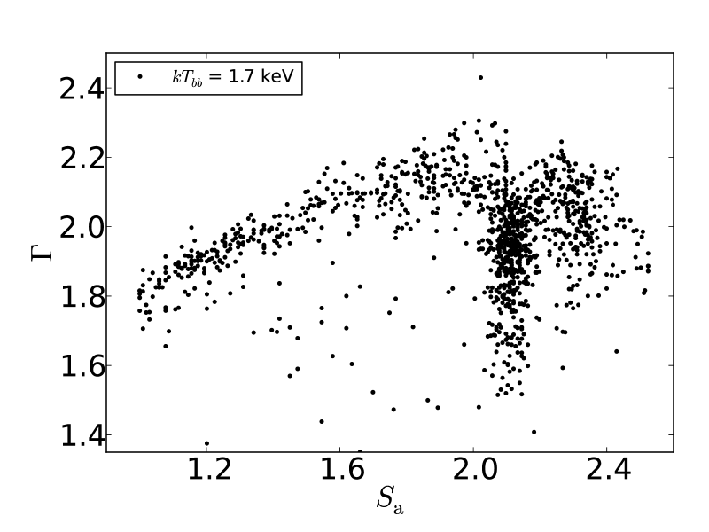
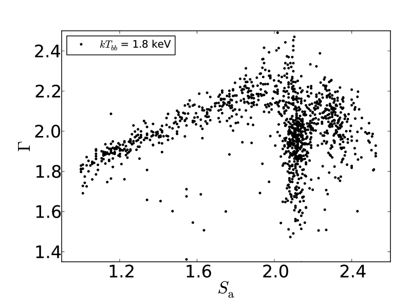
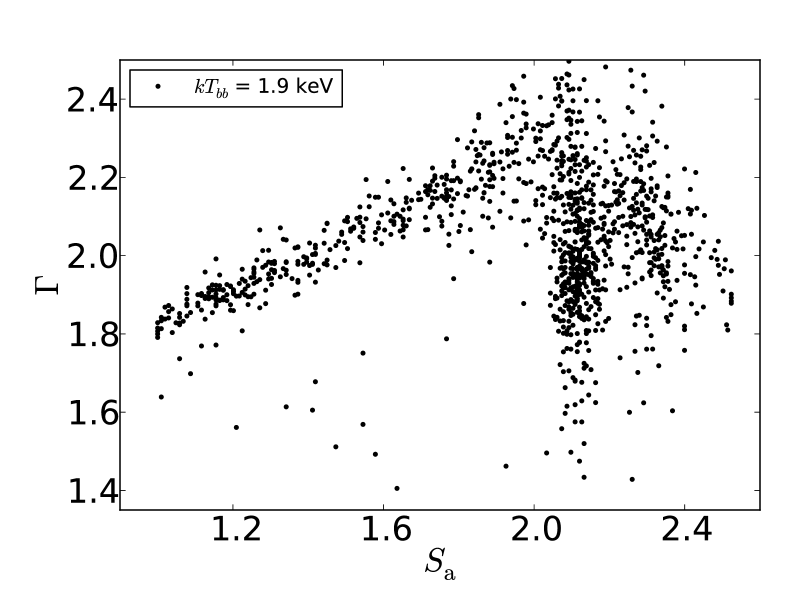
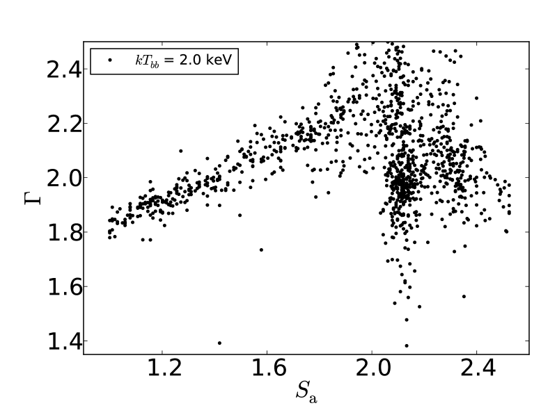
Figure 2: The power-law index, $\Gamma$, of the nthcomp component as a function of $S_{\rm a}$ in 4U 1636–53. The temperature of the blackbody component, $kT_{\rm bb}$, was fixed to the value indicated in each panel.

In order to visualise the evolution of the individual components and the total spectrum in different states, we chose four observations covering the whole range of $S_{\rm a}$ values. The four observations, Obs1, Obs2, Obs3 and Obs4 with $S_{\rm a}=$1.05, 1.90, 2.15 and 2.35, respectively, are shown with red filled circles in the upper panels of Figure 3. In the middle and lower panels of Figure 3 we show the PCA/HEXTE model spectra of these 4 observations. The spectral components in the plots are diskbb (red/dashed-dotted), bbodyrad (pink/dotted), gaussian (green/dotted) and nthcomp (blue dashed-three dotted), respectively. The best-fitting results for the four observations are given in Table 1.

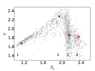
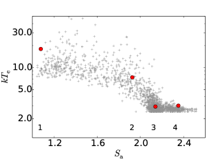
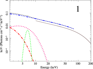
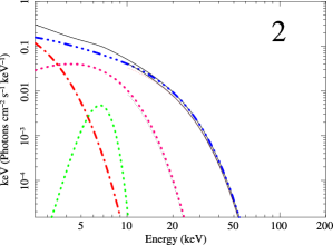
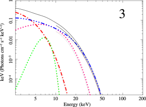
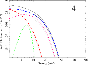
Figure 3: The upper left and right panels show, respectively, $\Gamma$ and $kT_{\rm e}$ of nthcomp as a function of $S_{\rm a}$ in 4U 1636–53. Each gray cross corresponds to an individual observation. The red circles indicate four observations at different positions in the CD. The middle and lower panels show, respectively, the total model spectrum and the individual spectral components of these four observations (middle-left, Obs1, middle-right, Obs2, bottom-left, Obs3, and bottom-right, Obs4). The spectral components in the plots are diskbb (red/dashed-dotted), bbodyrad (pink/dotted), gaussian (green/dotted) and nthcomp (blue dashed-three dotted), respectively. In each panel the solid black line represents the total model spectrum.

In the middle-left panel of Figure 3 (Obs1) the source is in the low/hard state. The broad band X-ray spectrum is dominated by the hard/Comptonised component, nthcomp. In this observation the power-law index is $\Gamma\sim 1.7$ and the electron temperature is $kT_{\rm e}\sim 17$ keV

When the source evolves from the low/hard state towards the vertex in the CD, the value of $S_{\rm a}$ increases from 1.0 to 2.0, $\Gamma$ increases from $\sim 1.7$ to $\sim 2.3$ and the spectrum becomes soft (Obs2 in the right panel of Figure 3). The electron temperature decreases from $kT_{\rm e}\sim 17$ keV to $\sim 8$ keV. Compared to Obs1, it is clear that the contribution of bbodyrad and diskbb increases, and the emission above 80 keV drops, significantly.

When the source is at the transitional state, $S_{\rm a}\sim 1.9-2.2$, the value of $\Gamma$ covers a large range between 1.3 and 2.5. The emission from the diskbb and nthcomp components is more or less the same below 5 keV (bottom left panel of Figure 3). The nthcomp component is relatively flat but the high-energy cut-off is at much lower energy than in Obs1. Our results are consistent with those of Sanna et al. (2013) for the combined XMM-Newton–RXTE spectra (see their Figure 4).

When the source moves out from the transitional state to the high-soft state (Obs4), similar to what Sanna et al. (2013) show in their Figure 4, the normalization of diskbb decreases and the emission from diskbb is lower than that of nthcomp below 5 keV.

Table 1: Best-fitting results for the four observations. The error bars are given in 1 $\sigma$ level.

Component	Parameter	Obs. 1	Obs. 2	Obs. 3	Obs. 4
diskbb	$kT_{\rm dbb}$ (keV)	0.30	0.60	0.75	0.80
	$N_{\rm dbb}$	550$\pm$320	120$\pm$70	115$\pm$ 35	165$\pm$85
bbody	$kT_{\rm bb}$ (keV)	1.33$\pm$0.12	1.75$\pm$0.28	2.05$\pm$0.27	1.72$\pm 0.65$
	$N_{\rm bb}$ ($10^{-3}$)	1.3$\pm$0.8	3.8$\pm$2.4	2.9${}^{+1.0}_{-0.4}$	6.2${}^{+0.5}_{-0.2}$
nthcomp	$\Gamma$	1.68$\pm$0.05	2.28$\pm$0.27	1.86$\pm$0.39	1.81$\pm$0.42
	$kT_{e}$ (keV)	17.1$\pm$6.1	8.2$\pm$4.7	2.9$\pm$0.4	3.1$\pm$0.5
	$N_{\rm NTH}$	0.17$\pm$0.02	0.12$\pm$0.04	0.31$\pm$0.09	0.19$\pm$0.07

3.2 X-ray spectral properties in the transitional state

From Figure 3 and the discussion above, it is apparent that the power-law photon index, $\Gamma$, in many of the observations shows a significant drop when the source is in the transitional state. Due to the large spread of $\Gamma$ when 2 $\mathrel{\mathchoice{\lower 0.5pt\vbox{\halign{$\mathnew\displaystyle\hfil#\hfil$\cr<\crcr\sim\crcr}}}{\lower 0.5pt\vbox{\halign{$\mathnew\textstyle\hfil#\hfil$\cr<\crcr\sim\crcr}}}{\lower 0.5pt\vbox{\halign{$\mathnew\scriptstyle\hfil#\hfil$\cr<\crcr\sim\crcr}}}{\lower 0.5pt\vbox{\halign{$\mathnew\scriptscriptstyle\hfil#\hfil$\cr<\crcr\sim\crcr}}}}$ $S_{\rm a}$ $\mathrel{\mathchoice{\lower 0.5pt\vbox{\halign{$\mathnew\displaystyle\hfil#\hfil$\cr<\crcr\sim\crcr}}}{\lower 0.5pt\vbox{\halign{$\mathnew\textstyle\hfil#\hfil$\cr<\crcr\sim\crcr}}}{\lower 0.5pt\vbox{\halign{$\mathnew\scriptstyle\hfil#\hfil$\cr<\crcr\sim\crcr}}}{\lower 0.5pt\vbox{\halign{$\mathnew\scriptscriptstyle\hfil#\hfil$\cr<\crcr\sim\crcr}}}}$ 2.2 the trend of $\Gamma$ in this area of the plot is not clear. We therefore first sorted the data in Figure 3 according to $S_{\rm a}$ and rebinned them using a step of 0.025, 0.005 and 0.02 in the range of 1.0$<S_{\rm a}<$1.8, 1.8$<S_{\rm a}<$2.2 and $S_{\rm a}>$2.2, respectively. The weighted average $\Gamma$ as a function of $S_{\rm a}$ is shown in Figure 4. From this Figure it is apparent that, as $S_{\rm a}$ increases from $\sim 2.0$ to $\sim 2.2$, $\Gamma$ decreases abruptly from $\sim 2.3$ to $\sim 1.5$, around $S_{\rm a}$ $\sim 2.2$ $\Gamma$ increases again with $S_{\rm a}$ from $\sim 1.5$ to $\sim 1.9$ and, as $S_{\rm a}$ increases from $\sim 2.2$ to $\sim 2.5$, $\Gamma$ decreases from $\sim 1.9$ to $\sim 1.7$. In the transitional state $\Gamma$ shows a large spread, but the plot in Figure 4 shows that $\Gamma$ changes significantly with $S_{\rm a}$ and that the variation of $\Gamma$ is larger than the statistical fluctuations in the data. The large range of $\Gamma$ at the transitional state might be due to the fact that the model assumptions (e.g., a geometrically thin disc, or a spherical corona) are no longer valid.

3.3 Relation between $\Gamma$ and the presence of the lower kHz QPO

Figure 5 shows the centroid frequency of all the kHz QPOs detected in 4U 1636–53 as a function of $S_{\rm a}$. The filled circles (black) and the filled squares (red) represent the observations with upper and lower kHz QPOs, respectively (see also Sanna et al., 2013). The upper kHz QPO is detected when $S_{\rm a}<2.3$, and its frequency increases as $S_{\rm a}$ increases. The lower kHz QPO however, is only detected when $1.9\mathrel{\mathchoice{\lower 0.5pt\vbox{\halign{$\mathnew\displaystyle\hfil#\hfil$\cr<\crcr\sim\crcr}}}{\lower 0.5pt\vbox{\halign{$\mathnew\textstyle\hfil#\hfil$\cr<\crcr\sim\crcr}}}{\lower 0.5pt\vbox{\halign{$\mathnew\scriptstyle\hfil#\hfil$\cr<\crcr\sim\crcr}}}{\lower 0.5pt\vbox{\halign{$\mathnew\scriptscriptstyle\hfil#\hfil$\cr<\crcr\sim\crcr}}}}S_{\rm a}\mathrel{\mathchoice{\lower 0.5pt\vbox{\halign{$\mathnew\displaystyle\hfil#\hfil$\cr<\crcr\sim\crcr}}}{\lower 0.5pt\vbox{\halign{$\mathnew\textstyle\hfil#\hfil$\cr<\crcr\sim\crcr}}}{\lower 0.5pt\vbox{\halign{$\mathnew\scriptstyle\hfil#\hfil$\cr<\crcr\sim\crcr}}}{\lower 0.5pt\vbox{\halign{$\mathnew\scriptscriptstyle\hfil#\hfil$\cr<\crcr\sim\crcr}}}}2.2$, and its frequency covers a broad range over a narrow $S_{\rm a}$ range.

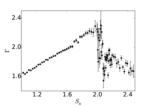
Figure 4: The power-law index, $\Gamma$, in nthcomp as a function of $S_{\rm a}$ in 4U 1636$-$53. The data are the same as in the upper left panel of Figure 3, but have been rebinned as described in the text.

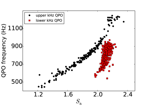
Figure 5: The kHz QPO frequency as a function of $S_{\rm a}$ in 4U 1636–53. The filled circles (black) and filled squares (red) represent the observations with upper and lower kHz QPOs, respectively.

In the upper panel of Figure 6 we plot the power-law photon index, $\Gamma$, as a function of $S_{\rm a}$ (the same data shown in Figure 3). The filled circles (black) and the filled squares (red) represent the observations with upper and lower kHz QPOs, respectively. Interestingly, observations with lower kHz QPOs correspond with those observations in which $\Gamma$ shows a large spread.

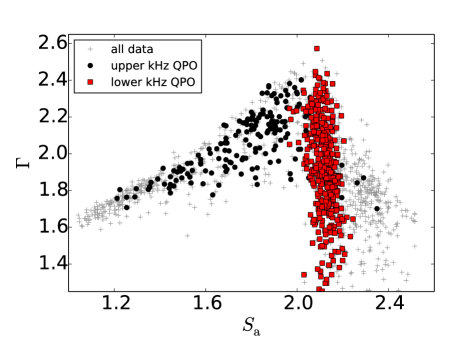
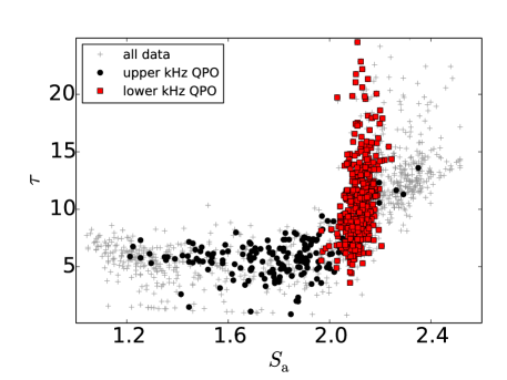
Figure 6: The upper and lower panels show, respectively, $\Gamma$ and $\tau$ as a function of $S_{\rm a}$ in 4U 1636–53. The filled circles (black) and filled squares (red) represent the observations with upper and lower kHz QPOs, respectively. The gray crosses represent observations in which no kHz QPO was detected.

In the case of Comptonisation in spherically symmetric region $\Gamma$ can be expressed as:

$$\Gamma=\left[\frac{9}{4}+\frac{1}{(kT_{e}/m_{e}c^{2})\tau(1+\tau/3)}\right]^{1/2}-\frac{1}{2},$$ (1)

where $\tau$ is the optical depth of the medium, and $kT_{e}$ is the electron temperature of the Comptonising region (Sunyaev & Titarchuk, 1980). We calculated $\tau$ for each observation and plotted them as a function of $S_{\rm a}$ in the lower panel of Figure 6. From this figure it is apparent that in the low/hard state the optical depth remains more or less constant at $\tau\sim 5$ as $S_{\rm a}$ increases from $\sim 1.0$ to $\sim 2.0$. When the source enters the transitional state, with $2.0\mathrel{\mathchoice{\lower 0.5pt\vbox{\halign{$\mathnew\displaystyle\hfil#\hfil$\cr<\crcr\sim\crcr}}}{\lower 0.5pt\vbox{\halign{$\mathnew\textstyle\hfil#\hfil$\cr<\crcr\sim\crcr}}}{\lower 0.5pt\vbox{\halign{$\mathnew\scriptstyle\hfil#\hfil$\cr<\crcr\sim\crcr}}}{\lower 0.5pt\vbox{\halign{$\mathnew\scriptscriptstyle\hfil#\hfil$\cr<\crcr\sim\crcr}}}}S_{\rm a}\mathrel{\mathchoice{\lower 0.5pt\vbox{\halign{$\mathnew\displaystyle\hfil#\hfil$\cr<\crcr\sim\crcr}}}{\lower 0.5pt\vbox{\halign{$\mathnew\textstyle\hfil#\hfil$\cr<\crcr\sim\crcr}}}{\lower 0.5pt\vbox{\halign{$\mathnew\scriptstyle\hfil#\hfil$\cr<\crcr\sim\crcr}}}{\lower 0.5pt\vbox{\halign{$\mathnew\scriptscriptstyle\hfil#\hfil$\cr<\crcr\sim\crcr}}}}2.2$, $\tau$ increases very abruptly with $S_{\rm a}$. In the observations with a lower kHz QPO $\tau$ covers the range from $\sim 5$ to $\sim 25$. A large value of $\tau$ has also been found in the soft state of other NS-LMXBs (e.g. 4U 1608$-$52 Gierliński & Done, 2002). The large variation of $\Gamma$ (and $\tau$) over a small region in the CD indicates that, in the transitional state, either the spectrum changes significantly or the model is no longer physically appropriate. Even if the latter was the case, it is still interesting that the lower kHz QPO is detected only in this part of the diagram.

4 Discussion

We fitted the $3-180$ keV X-ray spectra of all RXTE observations of the neutron-star low-mass X-ray binary 4U 1636–53 with a model that includes a Comptonised component. We subsequently studied the relation between the parameters of this component and the presence of kHz QPOs as a function of the source state, using the parameter $S_{\rm a}$ to measure the position of the source in the CD. We found that, while the upper kHz QPO is present in almost all states of the source, the lower kHz QPO appears only during the transition from the hard to the soft state, in observations in which the optical depth of the Comptonised component is relatively high and increases very sharply with $S_{\rm a}$, from $\tau\sim 5$ to $\tau\sim 25$.

In the low-hard state, the power-law index of the Comptonised component, $\Gamma$, increases gradually from $\Gamma\sim 1.6$ to $\Gamma\sim 2.3$ as the source spectrum softens and the source moves in the CD from the hard to the transitional state. In these observations $\Gamma$ is well correlated with the source hard colour and $S_{\rm a}$. The power density spectra of these observations show only the upper kHz QPO, with the QPO frequency being also correlated both with hard colour and $S_{\rm a}$. Similar correlations have been reported in other NS-LMXBs (e.g., 4U 0614+09, 4U 1608–52, 4U 1728–34, and Aql X–1; Kaaret et al., 1998; Méndez et al., 1999; Méndez & van der Klis, 1999; Méndez, 2000).

These correlations between spectral and timing properties in 4U 1636–53 are consistent with the scenario in which the truncation radius of the accretion disc decreases as mass accretion increases: As the X-ray luminosity of the source (and the inferred mass accretion rate through the disc) increases, the inner truncation radius of the accretion disc decreases (e.g. Done et al., 2007; Méndez et al., 1999, 2001; van Straaten et al., 2002; Altamirano et al., 2008) and the disc temperature (Shakura & Sunyaev, 1973), and hence the soft flux, in the system increases. This in turn boosts the cooling of the corona through inverse Compton scattering, which leads to a drop of the electron temperature and an increase of the optical depth of the corona (Gierliński & Done, 2002), and the energy spectrum of the source softens. In the case of 4U 1636–53 this picture is further supported by fits to the XMM-Newton and RXTE (PCA$+$HEXTE) spectra in the $0.8-200$ keV band over a range of source spectral states (Sanna et al., 2013; Lyu et al., 2014). Finally, if the frequency of the upper kHz QPO reflects the Keplerian frequency at the inner edge of the accretion disc, a smaller truncation radius yields a higher QPO frequency.

The above description only links the dynamics (frequency) of (at least) the upper kHz QPO to the spectral properties of the source, but it does not address the mechanism that determines the emission properties of the QPOs. For example, the steep increase of the rms amplitude of the kHz QPOs with energy (e.g., Berger et al., 1996; Méndez et al., 2001; Gilfanov et al., 2003) implies a modulation of the emitted flux of up to $\sim 20$% at $\sim 25-30$ keV, where the contribution of the disc is negligible (see Figure 3). Our findings suggest that the mechanisms that lead to the emission of the lower and the upper kHz QPO are not the same. This is similar to what was proposed by de Avellar et al. (2013) based on the energy and frequency dependence of the time lags of the kHz QPOs in this source. We detect the upper kHz QPO over all source spectral states, except the extreme soft state, whereas we only detect the lower kHz QPO in the transition from the hard to the soft state, at $S_{\rm a}\sim 1.9-2.2$, where $\Gamma$ drops abruptly from $\sim 2.3$ to $\sim 1.5$.

The parameter $\Gamma$, together with the electron temperature, $kT_{e}$, in the nthcomp spectral model component is related to $\tau$, the optical depth of the corona responsible for the Comptonised emission, through eq. (1). Since during the observations in the transitional state, where the lower kHz QPO is present, $\Gamma$ drops abruptly (see, e.g., the upper left panel of Figure 3), whereas $kT_{e}$ continues decreasing gradually (see the upper right panel of Figure 3), in the context of the nthcomp model the drastic changes of $\Gamma$ likely reflect substantial changes of the optical depth of the corona. The lower panel of Figure 6 shows that in the observations with the lower kHz QPO $\tau$ is high and increases very sharply with $S_{\rm a}$, from $\tau\sim 5$ to $\tau\sim 25$. Notwithstanding that in several of these observations we also detected the upper kHz QPO, this QPO is also present in observations in which the optical depth of the corona is low in comparison, $\tau\mathrel{\mathchoice{\lower 0.5pt\vbox{\halign{$\mathnew\displaystyle\hfil#\hfil$\cr<\crcr\sim\crcr}}}{\lower 0.5pt\vbox{\halign{$\mathnew\textstyle\hfil#\hfil$\cr<\crcr\sim\crcr}}}{\lower 0.5pt\vbox{\halign{$\mathnew\scriptstyle\hfil#\hfil$\cr<\crcr\sim\crcr}}}{\lower 0.5pt\vbox{\halign{$\mathnew\scriptscriptstyle\hfil#\hfil$\cr<\crcr\sim\crcr}}}}5$, and does not change much with $S_{\rm a}$.

Notice, by the way, that the drop of $\Gamma$ in the transitional and soft states does not contradict the fact that at $S_{\rm a}\geq 2$ the spectrum of the source softens. Indeed, although in the transitional and soft states $\Gamma$ decreases to values that are similar to those in the hard state, suggesting an overall hardening of the spectrum, $kT_{e}$ is much higher in the hard than in the transitional and soft states, such that the $3-180$ keV spectrum of the source does in fact softens as $S_{\rm a}$ increases (cf. Figure 3).

Lee et al. (2001) (see also Lee & Miller, 1998) proposed a model in which a feed-back loop between the corona and the source of soft photons (the disc and/or the neutron-star surface) excites a global mode in the system, such that the temperature and electron density of the corona and the temperature of the source of soft photons oscillate coherently at a given frequency, giving rise to a QPO. This model can explain the rms and time-lag energy spectra of the lower kHz QPO (Berger et al., 1996; Vaughan et al., 1997) in the NS LMXB 4U 1608–52. This scenario also provides a framework to interpret our findings in terms of a coupling and an efficient energy exchange between the disc and the corona. Since in the observations in which the lower kHz QPO is present the changes of the temperature of the corona are relatively small (at least compared to the relative changes of the optical depth), the frequency range spanned by this QPO likely reflects the range of optical depths (electron density) in the corona at which the resonance is excited.

We define the optical depth of the corona as $\tau=\sigma_{\rm T}n_{\rm e}l$ (Lee & Miller, 1998), where $l$ is the size of the corona, $\sigma_{\rm T}=6.65\times 10^{-25}$ cm² is the Thomson cross section of the electron, and $n_{\rm e}$ is the electron density. If we take 5 and 20 as extreme values of $\tau$ in our fits (see Figure 6), then $n_{\rm e}\approx$ $0.5-1.9\times 10^{19}$ cm^-3 and $2-7.5\times 10^{19}$ cm^-3 for $l$ in the range of 4 and 15 km (Lee et al., 2001), respectively. These values are consistent with the typical electron density in the corona of neutron star or black hole systems (e.g., Nobili et al., 2000).

It is interesting that in 4U 1636–53 the frequency at which (i) the lower kHz QPO is most often detected (Belloni et al., 2005), (ii) the quality factor ($Q$, defined as the QPO frequency divided by the full-width at half-maximum) of the lower kHz QPO is the highest (Barret et al., 2006), and (iii) the coherence between the low- and high-energy signals is the highest (de Avellar et al., 2013), is always $\sim 850$ Hz. Furthermore, de Avellar et al. (2016) recently showed that the phase lag between the low- and high-energy photons in the lower kHz QPO in 4U 1636–53 is largest at $S_{\rm a}\sim 2.1$, which also corresponds to a QPO frequency of $\sim 850$ Hz.

All the above suggests that this frequency corresponds to a global oscillation mode of the accretion flow in this source (see Lee et al., 2001). The mode could possibly be excited over a fairly large range of values of the properties of the corona (e.g., $\tau$, $kT_{e}$ and $l$), and hence over a range of frequencies of the QPO, as observed. On the other hand, the excitation and damping mechanisms of this global mode of the corona will play a role upon the range of frequencies and the coherence of the QPO. In a follow-up paper (Ribeiro et al. 2017, in preparation) we discuss correlations between the rms amplitude of the QPOs and the spectral properties of the source, which provide further support to this scenario.

References

- Altamirano et al. (2012) Altamirano D., Ingram A., van der Klis M., Wijnands R., Linares M., Homan J., 2012, ApJ, 759, L20
- Altamirano et al. (2008) Altamirano D., van der Klis M., Méndez M., Jonker P. G., Klein-Wolt M., Lewin W. H. G., 2008, ApJ, 685, 436
- Anders & Grevesse (1989) Anders E., Grevesse N., 1989, Geochim. Cosmochim. Acta, 53, 197
- Arnaud (1996) Arnaud K. A., 1996, in G. H. Jacoby & J. Barnes ed., Astronomical Data Analysis Software and Systems V Vol. 101 of Astronomical Society of the Pacific Conference Series, XSPEC: The First Ten Years. p. 17
- Balucinska-Church & McCammon (1992) Balucinska-Church M., McCammon D., 1992, ApJ, 400, 699
- Barret (2001) Barret D., 2001, Advances in Space Research, 28, 307
- Barret et al. (2006) Barret D., Olive J.-F., Miller M. C., 2006, MNRAS, 370, 1140
- Belloni et al. (2007) Belloni T., Homan J., Motta S., Ratti E., Méndez M., 2007, MNRAS, 379, 247
- Belloni et al. (2005) Belloni T., Méndez M., Homan J., 2005, A&A, 437, 209
- Berger et al. (1996) Berger M., van der Klis M., van Paradijs J., Lewin W. H. G., Lamb F., Vaughan B., Kuulkers E., Augusteijn T., Zhang W., Marshall F. E., Swank J. H., Lapidus I., Lochner J. C., Strohmayer T. E., 1996, ApJ, 469, L13
- de Avellar et al. (2016) de Avellar M. G. B., Méndez M., Altamirano D., Sanna A., Zhang G., 2016, MNRAS, 461, 79
- de Avellar et al. (2013) de Avellar M. G. B., Méndez M., Sanna A., Horvath J. E., 2013, MNRAS, 433, 3453
- Done et al. (2007) Done C., Gierliński M., Kubota A., 2007, A&A Rev., 15, 1
- Gierliński & Done (2002) Gierliński M., Done C., 2002, MNRAS, 337, 1373
- Gilfanov et al. (2003) Gilfanov M., Revnivtsev M., Molkov S., 2003, A&A, 410, 217
- Hasinger & van der Klis (1989) Hasinger G., van der Klis M., 1989, A&A, 225, 79
- Jahoda et al. (2006) Jahoda K., Markwardt C. B., Radeva Y., Rots A. H., Stark M. J., Swank J. H., Strohmayer T. E., Zhang W., 2006, ApJS, 163, 401
- Jonker et al. (2002) Jonker P. G., Méndez M., van der Klis M., 2002, MNRAS, 336, L1
- Kaaret et al. (1998) Kaaret P., Yu W., Ford E. C., Zhang S. N., 1998, ApJ, 497, L93
- Kluzniak & Abramowicz (2001) Kluzniak W., Abramowicz M. A., 2001, Acta Physica Polonica B, 32, 3605
- Kluźniak et al. (2004) Kluźniak W., Abramowicz M. A., Kato S., Lee W. H., Stergioulas N., 2004, ApJ, 603, L89
- Leahy et al. (1983) Leahy D. A., Darbro W., Elsner R. F., Weisskopf M. C., Kahn S., Sutherland P. G., Grindlay J. E., 1983, ApJ, 266, 160
- Lee & Miller (1998) Lee H. C., Miller G. S., 1998, MNRAS, 299, 479
- Lee et al. (2001) Lee H. C., Misra R., Taam R. E., 2001, ApJ, 549, L229
- Lin et al. (2007) Lin D., Remillard R. A., Homan J., 2007, ApJ, 667, 1073
- Lyu et al. (2014) Lyu M., Méndez M., Sanna A., Homan J., Belloni T., Hiemstra B., 2014, MNRAS, 440, 1165
- Méndez (2000) Méndez M., 2000, Nuclear Physics B Proceedings Supplements, 80, C1516
- Méndez (2006) Méndez M., 2006, MNRAS, 371, 1925
- Méndez & van der Klis (1999) Méndez M., van der Klis M., 1999, ApJ, 517, L51
- Méndez et al. (2001) Méndez M., van der Klis M., Ford E. C., 2001, ApJ, 561, 1016
- Méndez et al. (1999) Méndez M., van der Klis M., Ford E. C., Wijnands R., van Paradijs J., 1999, ApJ, 511, L49
- Miller et al. (1998) Miller M. C., Lamb F. K., Cook G. B., 1998, ApJ, 509, 793
- Nobili et al. (2000) Nobili L., Turolla R., Zampieri L., Belloni T., 2000, ApJ, 538, L137
- Plant et al. (2015) Plant D. S., Fender R. P., Ponti G., Muñoz-Darias T., Coriat M., 2015, A&A, 573, A120
- Rothschild et al. (1998) Rothschild R. E., Blanco P. R., Gruber D. E., Heindl W. A., MacDonald D. R., Marsden D. C., Pelling M. R., Wayne L. R., Hink P. L., 1998, ApJ, 496, 538
- Sanna et al. (2013) Sanna A., Hiemstra B., Méndez M., Altamirano D., Belloni T., Linares M., 2013, MNRAS, 432, 1144
- Sanna et al. (2012) Sanna A., Méndez M., Belloni T., Altamirano D., 2012, MNRAS, 424, 2936
- Shakura & Sunyaev (1973) Shakura N. I., Sunyaev R. A., 1973, A&A, 24, 337
- Stella & Vietri (1998) Stella L., Vietri M., 1998, ApJ, 492, L59
- Sunyaev & Titarchuk (1980) Sunyaev R. A., Titarchuk L. G., 1980, A&A, 86, 121
- van der Klis (2006) van der Klis M., 2006, Rapid X-ray Variability. pp 39–112
- van Straaten et al. (2002) van Straaten S., van der Klis M., di Salvo T., Belloni T., 2002, ApJ, 568, 912
- Vaughan et al. (1997) Vaughan B. A., van der Klis M., Méndez M., van Paradijs J., Wijnands R. A. D., Lewin W. H. G., Lamb F. K., Psaltis D., Kuulkers E., Oosterbroek T., 1997, ApJ, 483, L115
- Wijnands et al. (1997) Wijnands R. A. D., van der Klis M., van Paradijs J., Lewin W. H. G., Lamb F. K., Vaughan B., Kuulkers E., 1997, ApJ, 479, L141
- Zdziarski et al. (1996) Zdziarski A. A., Johnson W. N., Magdziarz P., 1996, MNRAS, 283, 193
- Zhang et al. (2009) Zhang G., Méndez M., Altamirano D., Belloni T. M., Homan J., 2009, MNRAS, 398, 368
- Zhang et al. (1997) Zhang W., Lapidus I., Swank J. H., White N. E., Titarchuk L., 1997, IAU Circ., 6541
- Życki et al. (1999) Życki P. T., Done C., Smith D. A., 1999, MNRAS, 309, 561