Vector resonances at LHC Run II
in composite 2HDM

Abstract

We consider a model where the electroweak symmetry breaking is driven by strong dynamics, resulting in an electroweak doublet scalar condensate, and transmitted to the standard model matter fields via another electroweak doublet scalar. At low energies the effective theory therefore shares features with a type-I two Higgs doublet model. However, important differences arise due to the rich composite spectrum expected to contain new vector resonances accessible at the LHC. We carry out a systematic analysis of the vector resonance signals at LHC and find that the model remains viable, but will be tightly constrained by direct searches as the projected integrated luminosity, around 200 fb^-1, of the current run becomes available.

I Introduction

Recently both the ATLAS and CMS collaborations updated the direct search limits on heavy vector resonances by using 13 TeV data with integrated luminosity ranging from 12.4 to 15.5 fb^-1 ATLAS:2016cyf ; ATLAS:2016ecs ; ATLAS:2016yqq ; ATLAS:2016cwq ; ATLAS:2016npe ; CMS:2016pfl ; CMS:2016abv . The resulting lower limits on sequential $W^{\prime}$ and $Z^{\prime}$ boson masses are about 4.7 and 4 TeV, respectively. The LHC reach for such heavy vector resonances is expected to further increase in the next analyses given that the integrated luminosity delivered by the LHC has reached about 45 fb^-1 at 13 TeV at the end of the 2016 run.

A traditional class of models requiring the existence of heavy vector resonances is technicolor (TC): the strong interaction responsible for a technifermion condensate breaking the electroweak (EW) symmetry generates also a rich spectrum of composite states whose mass is roughly fixed in the TeV range by the need to provide the observed masses to the $W^{\pm}$ and $Z$ gauge bosons. The observation of TeV scale vector resonances at LHC would therefore be a strong hint that technicolor is the underlying theory realized in Nature. The current mass limits are comparable to the typical TC scale, equal to about $4\pi v_{w}\simeq 3$ TeV, hence it is important to test the viability of TC theories and determine what portion of parameter space is soon to be explored, and whether a negative outcome of a heavy vector search could in principle rule out some of the currently viable theories in the TC framework.

In TC the Higgs couplings, which are constrained by LHC measurements within a few percent uncertainty, depend on the particular ultraviolet (UV) completion used to transmit EW symmetry breaking to the Standard Model (SM) fermion sector. To simplify the phenomenological analysis and its comparison with LHC data we choose a simple TC model as a template for more general extended TC theories. In the TC model at hand the interactions between the technifermions and SM fermions are mediated by an EW doublet scalar field Simmons:1988fu ; Dine:1990jd ; Samuel:1990dq ; Kagan:1990az ; Carone:1992rh ; Carone:1994mx (which we treat as elementary but can in principle be composite as well). The scalar sector of such UV complete model corresponds to that of a composite two Higgs doublet model (2HDM) Zerwekh:2009yu ; Antola:2009wq ; Alanne:2013dra ; DeCurtis:2016scv ; DeCurtis:2016tsm ; Agugliaro:2016clv ; Belyaev:2016ftv . Due to the strong interacting dynamics the model features a spectrum of higher-spin composite states, which distinguish this model from the ordinary type-I 2HDM. The main goal of this paper is to test the viability of this model given the LHC measurements of the light Higgs couplings to SM particles and LHC direct search constraints on heavy scalar and vector resonances, and to determine the expected reach of LHC Run II for the vector heavy states appearing in this model.

The paper is organized as follows: In section II we will first briefly introduce the model. In section III we update the fit of the model parameters to concur with the LHC data on the Higgs couplings, and in section IV we confront the signals of the vector resonances of the model with the current direct search constraints and present projections for the near future reach of the LHC experiments. Then in section V we offer our conclusions and a brief outlook for future research.

II Composite Vector Boson Interactions

The model we study, a composite 2HDM Antola:2009wq ; Alanne:2013dra , extends the particle content of the Next to Minimal Walking Technicolor (NMWT) Sannino:2004qp ; Dietrich:2005jn ; Belyaev:2008yj by a scalar field, $H$ (to be considered as a remnant of a UV complete theory, not necessarily strongly interacting), which features the same couplings as the SM Higgs field, and moreover couples to the technifermion fields via a renormalizable Yukawa interaction with coupling $y_{\rm TC}$. At an energy below the scale of the TC strong interaction, $\Lambda_{\rm TC}\sim 4\pi v_{w}\simeq 3$ TeV, the strongly interacting technifermions form a tower of composite states, analogously to QCD, whose interactions are encoded in an effective Lagrangian featuring the same global symmetries as the fundamental theory. The scalar sector of the 2HDM effective Lagrangian is expressed in terms of $H$ and a composite matrix scalar field $M$ as follows

$${\cal L}_{scalar} = \frac{1}{2}{\rm Tr}\!\left(D_{\mu}H^{\dagger}D^{\mu}H+D_{\mu}M^{\dagger}D^{\mu}M-m_{H}^{2}H^{\dagger}H-m_{M}^{2}M^{\dagger}M\right)$$ (1)

$$+ \left[\frac{y_{\rm TC}}{2}{\rm Tr}\!\left(c_{3}D_{\mu}M^{\dagger}D^{\mu}H+c_{1}f^{2}M^{\dagger}H\right)+\frac{c_{2}y_{\rm TC}}{24}{\rm Tr}(M^{\dagger}M){\rm Tr}(M^{\dagger}H)\right.$$

$$+ \left.\frac{c_{4}y_{\rm TC}}{24}\lambda_{H}{\rm Tr}(H^{\dagger}H){\rm Tr}(M^{\dagger}H)+{\textrm{h.c.}}\right]-\frac{\lambda_{H}}{24}{\rm Tr}\!\left(H^{\dagger}H\right)^{2}-\frac{\lambda_{M}}{24}{\rm Tr}\!\left(M^{\dagger}M\right)^{2},$$

with

$$H=\frac{1}{\sqrt{2}}\left(\phi I_{2\times 2}+i\pi_{H}^{k}\sigma_{k}\right)\,,\ \langle h\rangle=v\,,\quad M=\frac{1}{\sqrt{2}}\left(\varphi I_{2\times 2}+i\pi_{M}^{k}\sigma_{k}\right)\,,\ \langle s\rangle=f\,,\quad$$ (2)

and

$$D^{\mu}H=\partial^{\mu}H-ig_{L}W_{a}^{\mu}T^{a}H+ig_{Y}H\sigma_{3}\quad,\ D^{\mu}M=\partial^{\mu}M-ig_{L}W_{a}^{\mu}T^{a}M+ig_{Y}M\sigma_{3}\,,$$ (3)

where $\sigma_{k}$ are Pauli matrices. Contrary to the SM case, in composite 2HDM the squared mass term of the Higgs field $H$ is assumed to be positive (and generally of the order of the physical Higgs mass), so that EW symmetry breaking is triggered by the techniquark condensate $M$, with the EW scale determined in terms of the vevs of $M$ and $H$ by

$$v_{w}^{2}=v^{2}+f^{2}+2c_{3}y_{TC}fv=(246\ {\rm GeV})^{2}\,.$$ (4)

At lower order in $y_{\rm TC}$, considered to be perturbatively small, the composite vectors $A_{L}^{\mu}$ and $A_{R}^{\mu}$ couple only to the field $M$ Alanne:2013dra ,

$${\cal L}_{vector} = -\frac{1}{2}{\rm Tr}\!\left(\tilde{W}^{\mu\nu}\tilde{W}_{\mu\nu}\right)-\frac{1}{4}\tilde{B}^{\mu\nu}\tilde{B}_{\mu\nu}-\frac{1}{2}{\rm Tr}\!\left(F_{L}^{\mu\nu}F_{L\mu\nu}+F_{R}^{\mu\nu}F_{R\mu\nu}\right)+m_{A}^{2}{\rm Tr}\!\left(C_{L\mu}^{2}+C_{R\mu}^{2}\right)$$ (5)

$$-g^{2}_{\rm TC}r_{2}{\rm Tr}\!\left(C_{L\mu}MC^{\mu}_{R}M^{\dagger}\right)+\frac{g_{\rm TC}^{2}r_{1}}{4}{\rm Tr}\!\left(C_{L\mu}^{2}+C_{R\mu}^{2}\right){\rm Tr}\!\left(M^{\dagger}M\right)\ ,$$

with

$$C_{L}^{\mu}=A_{L}^{\mu}-\frac{g_{L}}{g_{\rm TC}}\tilde{W}^{\mu}\ ,\quad C_{R}^{\mu}=A_{R}^{\mu}-\frac{g_{Y}}{g_{\rm TC}}\tilde{B}^{\mu}\,,$$ (6)

where $\tilde{W}$ and $\tilde{B}$ are the SU$(2)_{L}$ and U$(1)_{Y}$ gauge fields, respectively. In Eq. (5) we neglected derivative couplings of the composite vectors given that these are anyway constrained to be small by the measured small values of the oblique parameters Peskin:1991sw ; Agashe:2014kda . The fermion sector is the same as that of the SM. The full Lagrangian, as defined in Eqs. (1)-(6), features the global symmetry SU$(2)_{L}\times$SU$(2)_{R}$, broken by the bosonic $y_{\rm TC}$ couplings in Eq. (1) Antola:2009wq ; Alanne:2013dra . This pattern reflects the global symmetry (and its breaking) of the strong sector of the NMWT fundamental Lagrangian Belyaev:2008yj ; Appelquist:1999dq ,

The vacuum expectation values (vev) of the $H$ and $M$ fields break the EW symmetry and give mass to both the SM and the TC states. The scalar sector can be recast in terms of a type-I 2HDM Alanne:2013dra , while the vector mass eigenstates are determined by diagonalizing the charged and neutral vector mass matrices given in Appendix A. The mass spectrum of the model, besides the SM particles, features one heavy Higgs, $h^{\prime}$, two mass degenerate pions, $a^{0}$ and $h^{\pm}$, and finally two charged and two neutral vector bosons, $W^{\prime\pm}$, $W^{\prime\prime\pm}$, and $Z^{\prime}$, $Z^{\prime\prime}$, respectively. The lightest charged vector boson, $W^{\pm}$, results from the mixing of the gauge field $\tilde{W}$ with composite vector fields that do not couple to SM fermions: consequentially the $W^{\pm}$ coupling to SM fermions is reduced. However, we checked that the Fermi coupling, $G_{F}$, determined by evaluating the tree level amplitude for the muon decay ($\mu^{-}\rightarrow\nu_{\mu}\bar{\nu}_{e}e^{-}$), respects the usual relation

$$\sqrt{2}G_{F}=v_{w}^{-2}=(246\,{\textrm{GeV}})^{-2}\ .$$ (7)

In the next section we perform a basic analysis of the phenomenological viability of composite 2HDM at LHC.

III Viable Phenomenology and the LHC fit

We express the scalar mass parameters $m_{M}$ and $m_{H}$ in terms of the remaining parameters by minimizing the scalar potential in Eq. (1) with respect to the vevs $f$ and $v$, which are determined by matching the experimental values of the EW scale, Eq. (4), and the Higgs mass, 125 GeV. The free parameters of the model are therefore $\lambda_{H}$, $\lambda_{M}$, $y_{\rm TC}$, $c_{1}$, $c_{2}$ ,$c_{3}$, $c_{4}$, from the scalar sector in Eq. (1), and $g_{\rm TC}$, $m_{A}$, $r_{1}$, and $r_{2}$, from the vector sector in Eq. (5). To assess the viability of the model, we scan the parameter space for data points that produce the observed SM mass spectrum, and satisfy the lower bounds on the scalar and pseudoscalar masses

$$m_{h^{\prime}}>600~{}{\rm GeV}\,;\ m_{a^{0}}\,,m_{h^{\pm}}>100~{}{\rm GeV}\,,$$ (8)

as well as the experimental bounds on the EW oblique parameters Peskin:1991sw ; Agashe:2014kda

$$S=0.00\pm 0.08\,,\ T=0.05\pm 0.07\,,\ \rho(S,T)=90\%\,.$$ (9)

The region of parameter space that we scan, as described in Alanne:2013dra , is limited by potential stability and perturbativity in $\lambda_{H}$, $\lambda_{M}$, and $y_{\rm TC}$, while the order of the coefficients $c_{i}$ is fixed by dimensional analysis Manohar:1983md . For the remaining vector sector parameters we choose values in the region, natural for TC,

$$500~{}{\rm GeV}<m_{A}<2500~{}{\rm GeV}\,,\ 2<g_{\rm TC}<6.5\,,\ r_{1}=-r_{2}={\cal O}(\frac{4m^{2}_{A}}{g^{2}_{\rm TC}f^{2}})\,,$$ (10)

where we impose the relation $r_{1}=-r_{2}$, which cancels the SM Higgs field coupling to the axial combination $A^{\mu}_{L}+A^{\mu}_{R}$, to simplify the phenomenological analysis without compromising the viability of the model.

Finally, we select the data points that satisfy the LHC constraints on the Higgs couplings to $W$, $Z$, $\gamma$, $b$, and $\tau$, as done in  Alanne:2013dra : for this purpose we calculate $\chi^{2}$ at each viable data point for the five Higgs coupling strengths, defined by

$$\hat{\mu}_{jj}=\frac{\sigma_{pp\rightarrow h(X)}\textrm{Br}_{jj}}{\sigma_{pp\rightarrow h(X)}^{\textrm{SM}}\textrm{Br}^{\textrm{SM}}_{jj}}\ ,\quad\textrm{Br}_{jj}=\frac{\Gamma_{h\rightarrow jj}}{\Gamma_{h}}\,,$$ (11)

where $X$ is a possible state produced in association with the light Higgs, and $jj$ a particle pair. The coupling strength values measured by both ATLAS and CMS ATLASCMSfit in inclusive processes are summarized in Table 1.

$jj$	ATLAS	CMS
$ZZ$	$\,1.52\pm 0.37\,$	$\,1.04\pm 0.29\,$
$\gamma\gamma$	$1.14\pm 0.26$	$1.11\pm 0.24$
$WW$	$1.22\pm 0.22$	$0.90\pm 0.22$
$\tau\tau$	$1.41\pm 0.38$	$0.88\pm 0.29$
$bb$	$0.62\pm 0.37$	$0.81\pm 0.44$

Table 1: Coupling strength experimental values determined by the ATLAS and CMS experiments.

The Higgs couplings relevant for this analysis are those of SM particles and new resonances, contributing to leading order loop couplings, whose coupling coefficients are defined by

$${\cal{L}}_{\textrm{eff}} \supset a_{V}\frac{2m_{W}^{2}}{v_{w}}hW^{+}_{\mu}W^{-\mu}+a_{V}\frac{m_{Z}^{2}}{v_{w}}hZ_{\mu}Z^{\mu}-a_{f}\sum_{\psi=t,b,\tau}\frac{m_{\psi}}{v_{w}}h\bar{\psi}\psi$$ (12)

$$+ a_{V^{\prime}}\frac{2m^{2}_{W^{\prime}}}{v_{w}}hW^{\prime+}_{\mu}W^{\prime-\mu}+a_{V^{\prime\prime}}\frac{2m^{2}_{W^{\prime\prime}}}{v_{w}}hW^{\prime\prime+}_{\mu}W^{\prime\prime-\mu}-a_{h}\frac{2m_{h^{\pm}}^{2}}{v_{w}}h\,h^{+}h^{-}\,,$$

where all the fields in the equation above are physical eigenstates. The coefficients of the SM Higgs linear couplings to matter fields in Eq. (12) can be expressed in terms of the Lagrangian parameters by

$$a_{h} = \left[\left(c_{2\beta}-c_{2\rho}\right)\left(\left(c_{2}-c_{4}\lambda_{H}\right)c^{-1}_{\rho}s^{-1}_{\rho}\left(c_{\alpha+3\beta}+c_{\alpha-\beta}c_{2\beta}c_{2\rho}\right)\right.\right.$$

$$+ \left.\left.4\left(c_{2}+c_{4}\lambda_{H}\right)c_{\beta}s_{\beta}\left(c_{\alpha}c_{\beta}t_{\rho}^{-2}+s_{\alpha}s_{\beta}t_{\rho}^{2}\right)\right)\right.$$

$$- \left.\left(c_{\alpha-\rho}s_{2(\beta-\rho)}^{2}s_{\beta+\rho}\lambda_{H}+c_{\alpha+\rho}s_{\beta-\rho}s_{2(\beta+\rho)}^{2}\lambda_{M}\right)c_{\rho}^{-2}s_{\rho}^{-2}/y_{TC}\right]$$

$$/ \left[4\left(c_{4}\lambda_{H}s_{\beta-\rho}^{2}+\left(12c_{1}+c_{2}\right)s_{\beta+\rho}^{2}\right)\right]\ ,$$

$$a_{f} = \frac{c_{\alpha-\rho}}{s_{\beta-\rho}}\ ,\quad s_{\rho}=\sqrt{\frac{1-c_{3}y_{TC}}{2}}\ ,\quad c_{\rho}=\sqrt{\frac{1+c_{3}y_{TC}}{2}}\,,$$ (13)

where $s_{\alpha},c_{\alpha},t_{\alpha}$ are shorthands for $\sin\alpha,\cos\alpha,\tan\alpha$, respectively, with $\alpha,\beta$ defined by the rotation matrices

$$\begin{pmatrix}h\\ h^{\prime}\end{pmatrix}=\begin{pmatrix}c_{\alpha}&-s_{\alpha}\\ s_{\alpha}&c_{\alpha}\end{pmatrix}\begin{pmatrix}\phi\\ \varphi\end{pmatrix}~{},\ \begin{pmatrix}G^{0}\\ a^{0}\end{pmatrix}=\begin{pmatrix}s_{\beta}&c_{\beta}\\ c_{\beta}&-s_{\beta}\end{pmatrix}\begin{pmatrix}\pi_{H}^{3}\\ \pi_{M}^{3}\end{pmatrix}\,.$$ (14)

The coupling coefficients of the charged vector resonances in Eq. (12) can be written in compact form by expanding at leading order correction in $\epsilon$ and $x$ as

$$a_{V}=\eta_{W}s_{\beta-\alpha}\ ,\quad a_{V^{\prime}}=\eta_{W^{\prime}}s_{\beta-\alpha}\ ,\quad a_{V^{\prime\prime}}=\eta_{W^{\prime\prime}}s_{\beta-\alpha}\ ,$$ (15)

where

$$\eta_{W} \cong 1-\frac{\left[1+s^{2}\left(3-\zeta\right)+2s^{4}\right]x^{2}\epsilon^{2}}{\left(1+2s^{2}\right)^{2}}\ ,\quad\eta_{W^{\prime}}\cong\frac{2\zeta s^{2}}{1+2s^{2}}+\frac{\left[1+2s^{2}\left(1-\zeta\right)\right]x^{2}\epsilon^{2}}{2\left(1+2s^{2}\right)^{2}}\ ,$$

$$\eta_{W^{\prime\prime}} \cong \frac{x^{2}\epsilon^{2}}{2}\,,$$ (16)

with

$$s\equiv\frac{g_{\rm TC}f}{2m_{A}}\sqrt{r_{1}}\ ,\quad x\equiv\frac{g_{L}v_{w}}{2m_{A}}\ ,\quad\epsilon\ \equiv\frac{g_{L}}{g_{\rm TC}}\ ,\quad\zeta=s_{\beta-\alpha}^{-1}\frac{c_{\alpha+\rho}}{s_{\beta+\rho}}\ .$$ (17)

As one can see from the last of Eqs. (III), the light Higgs coupling to $W^{\prime\prime}$ is negligible at leading order: this is a consequence of setting $r_{1}=-r_{2}$, Eqs. (10), which makes the mixing term between the axial composite vector field and the SM gauge field, Eq. (20), small in the limit of small $\epsilon$. Given that the heavier vector resonances couple to SM fermions only through the mixing with the SM gauge fields, also the $W^{\prime\prime}$ couplings to SM fermions are small. Finally, the same statements are true also for $Z^{\prime\prime}$, given that setting $r_{1}=-r_{2}$ in Eq. (19) makes the mixing term between axial and gauge vector fields small.

The charged non-SM particles in Eq. (12) contribute only to the diphoton decay, while the decay rates of SM particles get rescaled by the square of the corresponding coupling coefficient. We then select the data points satisfying the 90% confidence level (CL) constraint

$$P\left(\chi^{2}>\chi^{2}_{min}\right)>10\%$$ (18)

with 7 d.o.f., given that the number of observables is twelve while the effective free parameters is five. To see that the effective free parameters are just five one can notice that it is possible to fit simultaneously only five (three coupling strengths plus S and T) of the observables. Of the 10000 scanned data points satisfying perturbativity, potential stability, direct search constraints in Eqs. (8), and producing the observed SM mass spectrum, a total of 1381 points satisfy also the constraint in Eq. (18): in Fig. 1 these points are shown in green (68% CL) and blue (90% CL), while those in orange are viable with 95% CL, in the plane of the fermion and sum of the charged heavy vector resonances’ coupling coefficients.

Figure 1: Viable points at 68%,90%,95%CL shown in green, blue, orange in the plane of the coupling coefficients $a_{f}$ and $(a_{V^{\prime}}+a_{V^{\prime\prime}})$ as defined in Eq. (12).

As shown in Fig. 1, the experimentally favored values of the coupling coefficients lie close to one for fermions and to zero for the heavy vector resonances, as expected given that the measured values of the $W$, $Z$, $\gamma$, $b$, $\tau$ coupling strengths are SM-like. On the other hand the heavy neutral vector resonances are not directly constrained by the Higgs coupling strengths fit.

In the next section we use the collection of 1381 data points viable at 90% CL to analyze the phenomenology of both charged and neutral vector resonance production signals at the LHC.

IV LHC Signals

In order to compare the predictions of the composite 2HDM with the experimental results from the LHC, we implemented the model, defined by Eqs. (1,5) as well as by the SM fermion and QCD sectors, in the Monte Carlo event generator Madgraph Alwall:2014hca by using the Mathematica package Feynrules Christensen:2008py ; Alloul:2013bka . We have validated the implementation by checking that the values of the relevant couplings of the vector boson mass eigenstates evaluated with Madgraph at a sample data point matched the analytical result for the same values of the input parameters. We have performed the collider analysis at parton level, neglecting higher order effects such as parton showering, intial and final state radiation, and detector resolution. The most constraining final state turns out to be dimuon production for the neutral vector resonance, and charged lepton and neutrino for the charged vector resonance. These are electroweak processes and therefore are not too sensitive to QCD effects or NLO corrections. Furthermore, the uncertainty associated with our neglect of the detector resolution effects is mitigated by the fact that the experimental resolution for lepton momentum is very high. Thus we find it justifiable to perform the initial analysis at parton level. The relevant production channels we present here are the Drell-Yan production of a $Z^{\prime}$ subsequently decaying to a dilepton or a diboson, expressed by the Feynman diagrams in Fig. 2, and the production of a $W^{\prime}$ decaying to a charged lepton and a neutrino.

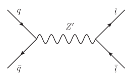
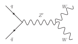
Figure 2: Feynman diagrams for the Drell-Yan production of a $Z^{\prime}$ subsequently decaying to a dilepton or a diboson.

The ATLAS dilepton search ATLAS:2016cyf looks for two opposite sign isolated charged leptons within the pseudorapidity window $|\eta|<2.5$. The corresponding production cross section evaluated with Madgraph at each of the 1381 collected data points is shown in Fig. 3 together with the upper limit (red solid line) from ATLAS:2016cyf and the projected limit with 45 fb^-1 (black dashed line) and 200 fb^-1 (black solid line). The color code of the data points corresponds to that of Fig. 1. We find that out of the scanned data points, 86% are already ruled out by the dilepton search, 94% can be ruled out with the currently existing data of 45 fb^-1, and 99% with the projected integrated luminosity of 200 fb^-1 for the current run. As explained above, we have limited the mass of the vector resonance to $m_{Z^{\prime}}\leq 2.5$ TeV, in order to stay safely below the TC confinement scale $\Lambda_{\rm TC}\sim 3$ TeV. Increasing further the composite vector boson masses, while generally allowed by naive dimensional analysis, would be less desirable based on naturalness arguments, which disfavor a large hierarchy between the confinement and the electroweak scales.

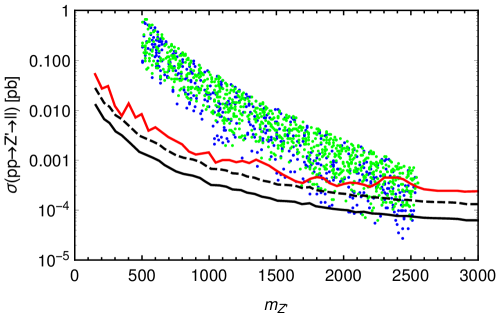
Figure 3: Upper bounds on the cross section for the Drell Yan production of a $Z^{\prime}$ subsequently decaying to a dilepton: the solid red line is the observed exclusion limit from ATLAS:2016cyf , the black dashed line shows the projected limit with 45 fb^-1, and the black solid line shows the projected limit with 200 fb^-1. The plot also shows the cross section for each of the 1381 viable data points evaluated with MadGraph. The color code of the data points corresponds to that of Fig. 1.

The most relevant constraint for the charged vector resonance $W^{\prime}$ is given by the search for a charged lepton and missing energy ATLAS:2016ecs . This search selects events with a single muon with transverse momentum $p_{T}>55$ GeV or a single electron with $p_{T}>65$ GeV in the pseudorapidity window $|\eta|<2.5$ for the muons and $|\eta|<2.47$ for the electrons. Additionally, the events must contain significant missing energy, $\not{E}_{T}>55$ GeV in the muon channel and $\not{E}_{T}>65$ GeV in the electron channel, and the transverse mass of the charged lepton plus neutrino system must be above 110 GeV in the muon channel and above 130 GeV in the electron channel. The corresponding cross section as a function of the $W^{\prime}$ mass for the data points is shown in figure 4, together with the constraint from ATLAS:2016ecs . The expected exclusion limits for 45 fb^-1 and 200 fb^-1 are shown by the black dashed and solid lines, respectively. We find that 90% of the scanned data points are already ruled out by the $W^{\prime}$ search, 98% can be ruled out with the data set of 45 fb^-1 and nearly all (99.8%) of the scanned parameter space points are within reach with 200 fb^-1.

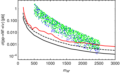
Figure 4: Upper bounds on the cross section for the production of a $W^{\prime}$ subsequently decaying to a charged lepton and a neutrino: the solid red line is the observed exclusion limit from ATLAS:2016ecs , the black dashed line shows the projected limit with 45 fb^-1, and the black solid line shows the projected limit with 200 fb^-1. The plot also shows the cross section for each of the 1381 viable data points evaluated with MadGraph. The color code of the data points corresponds to that of Fig. 1.

The limit on the diboson channel is less tight, as can be seen from Fig. 5, and most of the scanned data points are below the current limit ATLAS:2016cwq , shown by the red solid line. The expected exclusion limits for 45 fb^-1 (black dashed line) and for 200 fb^-1 (black solid line) reach larger portions of the data points, but all of these points are already ruled out by the dilepton search. From the color code of the data points in figures 3, 4 and 5 one can see that the lower $\chi^{2}$ points shown in green tend to have a higher production cross section. This feature seems more pronounced in the diboson channel, but is present also in the dilepton and lepton plus neutrino channels.

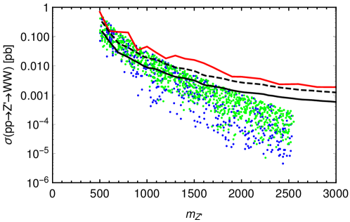
Figure 5: Upper bounds on the cross section for the Drell Yan production of a $Z^{\prime}$ subsequently decaying to $WW$: the solid red line is the observed exclusion limit from ATLAS:2016cwq , the black dashed line shows the projected limit with 45 fb^-1, and the black solid line shows the projected limit with 200 fb^-1. The plot also shows the cross section for each of the 1381 viable data points evaluated with MadGraph. The color code of the data points corresponds to that of Fig. 1.

V Conclusions and outlook

The latest LHC direct searches of heavy vector resonances ATLAS:2016cyf ; ATLAS:2016ecs ; ATLAS:2016yqq ; ATLAS:2016cwq ; ATLAS:2016npe ; CMS:2016pfl ; CMS:2016abv have an energy reach comparable to the TC scale ($\sim 3$ TeV), and their constraints are therefore relevant for TC models. In this paper we briefly reviewed a template TC model for which EW symmetry breaking, triggered by the new TC strong interaction between EW doublet technifermions, is transmitted to SM fermions via a scalar field coupling the TC matter sector to the SM one. The model features two (partially) composite Higgs bosons and several new heavy vector bosons, which are fully composite states and represent a clear signature common to all TC models Andersen:2011yj . We tested the viability of this model first of all by performing a fit of the lighter Higgs scalar couplings to SM vector bosons, bottom quarks, and tau leptons. We performed the goodness of fit analysis by scanning the model’s parameter space for data points producing a viable SM particle mass spectrum, and selecting those points that satisfy at 90% CL the experimental constraints on those couplings as well as the lower bound on the mass of a heavy Higgs scalar. The selected data set consists of 1381 viable data points. We then implemented the model in the event generator Madgraph Alwall:2014hca and calculated, for each viable data point, the cross section at the parton level for the dilepton and diboson channels of Drell-Yan production of heavy neutral vector bosons, and lepton plus neutrino channel for the production of a charged vector boson at the LHC. By comparing these results with the latest LHC constraints we showed that a major portion of the otherwise viable data points is already excluded by the direct searches of heavy vector resonances in the dilepton and lepton plus neutrino channels, while almost the entire parameter space we have considered will be tested by the end of LHC Run II in 2022. On the other hand the experimental constraints on the diboson channel are less tight as they are able to rule out only a smaller portion of the selected data set. These results show that the LHC experiments have the potential to discover signatures of TC in direct resonant production channels. Alternatively, if no new heavy vector boson resonances are discovered, very stringent constraints will be imposed on the TC framework of the type we have considered here, as a significant portion of parameter space naturally selected by naive dimensional analysis would be ruled out.

Heavy vector boson direct searches at the ATLAS and CMS experiments can in principle complement flavor experiments carried out at LHCb, whose 2015 data show large deviations from the SM predictions in flavor violating observables which might well be explained by a new heavy neutral vector particle Altmannshofer:2015sma ; Descotes-Genon:2015uva ; Hurth:2016fbr ; Gauld:2013qba . Flavor violating interaction terms in extended TC models are a natural by-product of fermion mass terms, and therefore would be a well motivated extension of the present template TC model.

Appendix A Vector Mass Matrices

The neutral vector squared mass matrix, obtained from Eq. (5), is

$${\cal M}_{Z}^{2}=\left(\begin{array}[]{cccc}\epsilon^{2}m_{A}^{2}t_{\theta}^{2}+m_{\tilde{W}}^{2}\left(z_{1}+1\right)t_{\theta}^{2}&-m_{\tilde{W}}^{2}\left(z_{2}+1\right)t_{\theta}&-\frac{\epsilon t_{\theta}m_{A}^{2}}{\sqrt{2}}-\frac{m_{\tilde{W}}^{2}\left(z_{1}-z_{2}\right)t_{\theta}}{\sqrt{2}\epsilon}&\frac{\epsilon t_{\theta}m_{A}^{2}}{\sqrt{2}}+\frac{m_{\tilde{W}}^{2}\left(z_{1}+z_{2}\right)t_{\theta}}{\sqrt{2}\epsilon}\\ -m_{\tilde{W}}^{2}\left(z_{2}+1\right)t_{\theta}&\epsilon^{2}m_{A}^{2}+m_{\tilde{W}}^{2}\left(z_{1}+1\right)&-\frac{\epsilon m_{A}^{2}}{\sqrt{2}}-\frac{m_{\tilde{W}}^{2}\left(z_{1}-z_{2}\right)}{\sqrt{2}\epsilon}&-\frac{\epsilon m_{A}^{2}}{\sqrt{2}}-\frac{m_{\tilde{W}}^{2}\left(z_{1}+z_{2}\right)}{\sqrt{2}\epsilon}\\ -\frac{\epsilon t_{\theta}m_{A}^{2}}{\sqrt{2}}-\frac{m_{\tilde{W}}^{2}\left(z_{1}-z_{2}\right)t_{\theta}}{\sqrt{2}\epsilon}&-\frac{\epsilon m_{A}^{2}}{\sqrt{2}}-\frac{m_{\tilde{W}}^{2}\left(z_{1}-z_{2}\right)}{\sqrt{2}\epsilon}&m_{A}^{2}+\frac{m_{\tilde{W}}^{2}\left(z_{1}-z_{2}\right)}{\epsilon^{2}}&0\\ \frac{\epsilon t_{\theta}m_{A}^{2}}{\sqrt{2}}+\frac{m_{\tilde{W}}^{2}\left(z_{1}+z_{2}\right)t_{\theta}}{\sqrt{2}\epsilon}&-\frac{\epsilon m_{A}^{2}}{\sqrt{2}}-\frac{m_{\tilde{W}}^{2}\left(z_{1}+z_{2}\right)}{\sqrt{2}\epsilon}&0&m_{A}^{2}+\frac{m_{\tilde{W}}^{2}\left(z_{1}+z_{2}\right)}{\epsilon^{2}}\end{array}\right)\,,$$ (19)

and the charged vector squared mass matrix is

$${\cal M}_{W}^{2}=\left(\begin{array}[]{ccc}\epsilon^{2}m_{A}^{2}+m_{\tilde{W}}^{2}\left(z_{1}+1\right)&-\frac{\epsilon m_{A}^{2}}{\sqrt{2}}-\frac{m_{\tilde{W}}^{2}\left(z_{1}-z_{2}\right)}{\sqrt{2}\epsilon}&-\frac{\epsilon m_{A}^{2}}{\sqrt{2}}-\frac{m_{\tilde{W}}^{2}\left(z_{1}+z_{2}\right)}{\sqrt{2}\epsilon}\\ -\frac{\epsilon m_{A}^{2}}{\sqrt{2}}-\frac{m_{\tilde{W}}^{2}\left(z_{1}-z_{2}\right)}{\sqrt{2}\epsilon}&m_{A}^{2}+\frac{m_{\tilde{W}}^{2}\left(z_{1}-z_{2}\right)}{\epsilon^{2}}&0\\ -\frac{\epsilon m_{A}^{2}}{\sqrt{2}}-\frac{m_{\tilde{W}}^{2}\left(z_{1}+z_{2}\right)}{\sqrt{2}\epsilon}&0&m_{A}^{2}+\frac{m_{\tilde{W}}^{2}\left(z_{1}+z_{2}\right)}{\epsilon^{2}}\end{array}\right)\,,$$ (20)

where

$$m_{\tilde{W}}=\frac{g_{L}v_{w}}{2}\ ,\quad t_{\theta}=\frac{g_{Y}}{g_{L}}\ ,\quad z_{1}=\frac{f^{2}}{v_{w}^{2}}r_{1}\ ,\quad z_{2}=\frac{f^{2}}{v_{w}^{2}}r_{2}\,,$$ (21)

while the remaining quantities are defined in Eqs. (17).

References

- (1) The ATLAS collaboration, ATLAS-CONF-2016-045.
- (2) The ATLAS collaboration, ATLAS-CONF-2016-061.
- (3) The ATLAS collaboration, ATLAS-CONF-2016-055.
- (4) The ATLAS collaboration, ATLAS-CONF-2016-062.
- (5) The ATLAS collaboration, ATLAS-CONF-2016-082.
- (6) CMS Collaboration, CMS-PAS-B2G-16-020.
- (7) CMS Collaboration, CMS-PAS-EXO-16-031.
- (8) E. H. Simmons, Nucl. Phys. B 312, 253 (1989).
- (9) M. Dine, A. Kagan and S. Samuel, Phys. Lett. B 243, 250 (1990).
- (10) S. Samuel, Nucl. Phys. B 347, 625 (1990).
- (11) A. Kagan and S. Samuel, Phys. Lett. B 252, 605 (1990); A. Kagan and S. Samuel, Phys. Lett. B 270, 37 (1991); A. Kagan and S. Samuel, Phys. Lett. B 284, 289 (1992); A. Kagan and S. Samuel, Int. J. Mod. Phys. A 7, 1123 (1992).
- (12) C. D. Carone and E. H. Simmons, Nucl. Phys. B 397, 591 (1993) [arXiv:hep-ph/9207273]; C. D. Carone and H. Georgi, Phys. Rev. D 49, 1427 (1994) [arXiv:hep-ph/9308205].
- (13) C. D. Carone, E. H. Simmons and Y. Su, Phys. Lett. B 344, 287 (1995) [arXiv:hep-ph/9410242].
- (14) B. Gripaios, A. Pomarol, F. Riva and J. Serra, JHEP 0904, 070 (2009) doi:10.1088/1126-6708/2009/04/070 [arXiv:0902.1483 [hep-ph]].
- (15) A. R. Zerwekh, Mod. Phys. Lett. A 25, 423 (2010) doi:10.1142/S0217732310032627 [arXiv:0907.4690 [hep-ph]].
- (16) M. Antola, M. Heikinheimo, F. Sannino and K. Tuominen, JHEP 1003, 050 (2010) [arXiv:0910.3681 [hep-ph]].
- (17) T. Alanne, S. Di Chiara and K. Tuominen, JHEP 1401, 041 (2014) [arXiv:1303.3615 [hep-ph]].
- (18) S. De Curtis, S. Moretti, K. Yagyu and E. Yildirim, Phys. Rev. D 94, 055017 (2016) doi:10.1103/PhysRevD.94.055017 [arXiv:1602.06437 [hep-ph]].
- (19) A. Agugliaro, O. Antipin, D. Becciolini, S. De Curtis and M. Redi, arXiv:1609.07122 [hep-ph].
- (20) S. De Curtis, S. Moretti, K. Yagyu and E. Yildirim, arXiv:1610.02687 [hep-ph].
- (21) A. Belyaev, G. Cacciapaglia, H. Cai, G. Ferretti, T. Flacke, A. Parolini and H. Serodio, arXiv:1610.06591 [hep-ph].
- (22) F. Sannino and K. Tuominen, Phys. Rev. D 71, 051901 (2005) doi:10.1103/PhysRevD.71.051901 [hep-ph/0405209].
- (23) D. D. Dietrich, F. Sannino and K. Tuominen, Phys. Rev. D 72, 055001 (2005) doi:10.1103/PhysRevD.72.055001 [hep-ph/0505059]. Belyaev:2008yj
- (24) A. Belyaev, R. Foadi, M. T. Frandsen, M. Jarvinen, F. Sannino and A. Pukhov, Phys. Rev. D 79, 035006 (2009) [arXiv:0809.0793 [hep-ph]].
- (25) M. E. Peskin and T. Takeuchi, Phys. Rev. D 46, 381 (1992).
- (26) K. A. Olive et al. [Particle Data Group Collaboration], Chin. Phys. C 38, 090001 (2014). Appelquist:1999dq
- (27) T. Appelquist, P. S. Rodrigues da Silva and F. Sannino, Phys. Rev. D 60, 116007 (1999) [hep-ph/9906555].
- (28) A. Manohar and H. Georgi, Nucl. Phys. B 234, 189 (1984).
- (29) The ATLAS and CMS Collaborations, ATLAS-CONF-2015-044.
- (30) J. Alwall et al., JHEP 1407, 079 (2014) doi:10.1007/JHEP07(2014)079 [arXiv:1405.0301 [hep-ph]].
- (31) N. D. Christensen and C. Duhr, Comput. Phys. Commun. 180, 1614 (2009) doi:10.1016/j.cpc.2009.02.018 [arXiv:0806.4194 [hep-ph]].
- (32) A. Alloul, N. D. Christensen, C. Degrande, C. Duhr and B. Fuks, Comput. Phys. Commun. 185, 2250 (2014) doi:10.1016/j.cpc.2014.04.012 [arXiv:1310.1921 [hep-ph]].
- (33) J. R. Andersen et al., Eur. Phys. J. Plus 126, 81 (2011) doi:10.1140/epjp/i2011-11081-1 [arXiv:1104.1255 [hep-ph]].
- (34) R. Gauld, F. Goertz and U. Haisch, Phys. Rev. D 89, 015005 (2014) doi:10.1103/PhysRevD.89.015005 [arXiv:1308.1959 [hep-ph]].
- (35) W. Altmannshofer and D. M. Straub, arXiv:1503.06199 [hep-ph].
- (36) S. Descotes-Genon, L. Hofer, J. Matias and J. Virto, JHEP 1606, 092 (2016) doi:10.1007/JHEP06(2016)092 [arXiv:1510.04239 [hep-ph]].
- (37) T. Hurth, F. Mahmoudi and S. Neshatpour, Nucl. Phys. B 909 (2016) 737 doi:10.1016/j.nuclphysb.2016.05.022 [arXiv:1603.00865 [hep-ph]].