The little-studied cluster Berkeley 90. III. Cluster parameters

Abstract

The open cluster Berkeley 90 is the home to one of the most massive binary systems in the Galaxy, LS III $+46\degr$11, formed by two identical, very massive stars (O3.5 If* + O3.5 If*), and a second early-O system (LS III $+46\degr$12 with an O4.5 IV((f)) component at least). Stars with spectral types earlier than O4 are very scarce in the Milky Way, with no more than 20 examples. The formation of such massive stars is still an open question today, and thus the study of the environments where the most massive stars are found can shed some light on this topic. To this aim, we determine the properties and characterize the population of Berkeley 90 using optical, near-infrared and WISE photometry and optical spectroscopy. This is the first determination of these parameters with accuracy. We find a distance of $3.5^{+0.5}_{-0.5}$ kpc and a maximum age of 3 Ma. The cluster mass is around $1\,000\>$M_☉ (perhaps reaching $1\,500\>$M_☉ if the surrounding population is added), and we do not detect candidate runaway stars in the area. There is a second population of young stars to the Southeast of the cluster that may have formed at the same time or slightly later, with some evidence for low-activity ongoing star formation.

1 Introduction

How do massive stars form? A number of different hypotheses have been put forth along time to try to circumvent the obvious physical difficulties that the formation of a very massive star presents (Zinnecker & Yorke, 2007, for a review). At present, two main theories are invoked: (a) monolithic core accretion, basically a scaled-up version of classical low-mass formation theories, where very high opacities allow infalling material to overcome the radiation pressure (e.g. Yorke & Sonnhalter, 2002; Krumholz et al., 2009) and (b) competitive accretion, where massive stars are formed in cluster cores, benefiting from the gravitational potential of the whole cluster to accrete more material (e.g. Bonnell & Bate, 2006; Smith et al., 2009).

The validity of these theories must be supported by the results of observations. The idea of competitive accretion stems naturally from the widespread evidence that massive stars are found mostly in young clusters. Because of their rarity, simple statistical arguments would suggest that they should preferentially be found in the most massive clusters (Elmegreen, 1983). Indeed, observations of clusters show that, in general, the mass of the most massive cluster member is a function of the cluster mass (Larson, 1995; Elmegreen, 1983; Weidner et al., 2010). However, it is still unclear if this is simply a consequence of statistical sampling of the initial mass function (IMF) or a consequence of a deeper underlying principle (resulting in sorted sampling; Weidner et al., 2013). Moreover, there is direct evidence of discs around some moderately massive stars (up to $M_{*}\sim 25$–30 M_☉; see Beltrán & de Wit, 2016, for a review), supporting the idea of monolithic collapse. On the other hand, massive stars in young clusters seem to lie in the regions of highest stellar density (Rivilla et al., 2013, 2014), a key prediction of the competitive accretion scenario that seems at odds with monolithic collapse.

One of the key observations that may help clarify theories of massive star formation is the degree of isolation under which massive stars can be formed (Lamb et al., 2010). Oey et al. (2013) presented a sample of 14 OB stars in the Small Magellanic Cloud (SMC) which meet strong criteria for having formed under extremely sparse star-forming conditions in the field. As this study was performed in the SMC (at a distance modulus of almost 19 mag), the stars observed can be safely claimed to be free of bright neighbours, but may still have a substantial complement of low-mass stars. In the Milky Way, similar observations can reach fainter magnitudes and thus imply certainty of isolation (e.g. de Wit et al., 2004). Characterization of the environment of very massive stars is a powerful tool not only to investigate their formation process, but also to understand how the IMF is sampled.

In this context, this is the third paper in a series of publications relating to the open cluster Berkeley 90 to study different astrophysical issues. Maíz Apellániz et al. (2015a, from now on, Paper I) characterized the two brightest stars in the cluster: LS III $+46\degr$11 and LS III $+46\degr$12. The former was identified as a new very early O-type spectroscopic binary (O3.5 If* + O3.5 If*), while the latter was classified as O4.5 V((f)) and suspected of binarity. In addition, orbital parameters for LS III $+46\degr$11 were derived by using multiepoch optical spectra, finding that it is composed by two very similar stars in a highly eccentric 97.3 d orbit. Moreover, LS III $+46\degr$11 is one of only six objects in the Northern hemisphere with spectral type earlier than O4 (Maíz Apellániz et al., 2016). The luminosity classification of LS III $+46\degr$12 was changed from V to IV in Maíz Apellániz et al. (2016), with the introduction of this new luminosity subclass. In Paper II (Maíz Apellániz et al., 2015b), the ISM sightlines towards LS III $+46\degr$11, LS III $+46\degr$12 and another B-type member (there named LS III $+46\degr$11B) were studied, with the conclusion that the absorbing ISM has at least two clouds at different velocities: one with a lower column density (thinner) in the K i lines located away from Berkeley 90 with velocity $\approx-7\>$km$\,\textrm{s}^{-1}$, and a second one with a higher column density (thicker), perhaps close to the cluster, with velocity $\approx-20\>$km$\,\textrm{s}^{-1}$.

There is very little previous information about the open cluster Berkeley 90 itself. As a result of a systematic inspection of the Palomar Sky Survey plates, Setteducati & Weaver (1962) identified 91 new open clusters that in the subsequent literature were named Berkeley clusters, where the majority of the stars are fainter than 13th magnitude. Berkeley 90 is an open cluster located within the isolated H ii region Sh2-115 ($l=84\aas@@fstack{\circ}9$), away from the Galactic plane ($b=+3\aas@@fstack{\circ}94$). Sanduleak (1974) was the first author to notice the presence of two OB stars (LS III $+46\degr$11 and LS III $+46\degr$12) in Berkeley 90. The first study of the cluster using 2MASS photometry and proper motions from NOMAD (Naval Observatory Merged Astrometric Dataset) was conducted by Tadross (2008), who obtained a new centre of coordinates ($\alpha$(J2000) = 20h 35m 17s, $\delta$(J2000)=$+46\degree$ $50\arcmin$ $06\arcsec$), and estimated a diameter of $5\arcmin$, an age of 0.1 Ga (clearly too old for a cluster containing OB stars), a reddening of $E(B-V)=1.15$ mag, and a distance of $2430\pm 70$ pc.

In this paper, we present optical and near-infrared (near-IR) photometry for Be 90, and optical spectroscopy for most of the cluster members in the upper main sequence. With this dataset, we are able to determine the parameters of the cluster with better accuracy and estimate the mass of the cluster, thus characterizing the properties and population of a small cluster hosting one of the most massive systems in the Galaxy. Furthermore, to understand the cluster formation process, we investigate its surroundings. For this purpose, we carry out the same study for a region to the southwest of the cluster, where bright-rimmed clouds are present. This area contains substantial amounts of gas and dust.

The paper is divided following this structure: in Section 2, we present the observations and reduction procedures used; in Section 3 we determine the parameters of the cluster and characterize its population, and in Section 4 we calculate the mass of the cluster, look for the existence of possible runaway stars and study the environment of other O3-type stars in the Galaxy. Finally, we list the conclusions.

2 Observations and data

We used the imager and spectrograph Andalucía Faint Object Spectrograph and Camera (ALFOSC) on the Nordic Optical Telescope (NOT) at the La Palma observatory to obtain $UBVR$ photometry on the night of 2007 July 9, and spectroscopy of 20 selected stars on the nights of 2004 October 4, 2005 October 2 – 4, and 2007 July 10. We also downloaded UKIDSS (Lawrence et al., 2007) images in the $JHK_{{\textrm{S}}}$ filters to perform deep near-IR photometry.

2.1 Spectroscopy

In spectroscopic mode, we used grisms #14 and #16 combined with a range of slit widths adapted to the weather conditions (between 1$\arcsec$ and 1.8$\arcsec$) to obtain intermediate resolution spectroscopy in the classification region. Grism #14 covers the 3275 – 6125 Å  range with a nominal dispersion 1.4 Å/pixel. Grism #16 covers the 3500 – 5060 Å  range with a nominal dispersion of 0.8 Å/pixel. The reduction procedure is the same as used in section 2.2 of Marco & Negueruela (2011). We observed selected bright stars in the zone and a number of objects in the central concentration whose 2MASS colours suggested membership applying criteria from Negueruela & Schurch (2007). We can see in Table 1 the names of the 20 observed stars (+2 stars from the literature) and their date of observation.

For one star (later named star 238) that presented photometric characteristics typical of an early-type emission line star, we obtained a moderately-high resolution spectrum in the H$\alpha$ region using the VPH grism #17. This grism covers the 6330 – 6870 Å range with a nominal dispersion of 0.26 Å/pixel.

Table 1: Stars with classification spectra taken with ALFOSC. Top panel are stars considered members and bottom panel are non-members stars

RA(J2000)	DEC(J2000)	Name	Spectral type	Date of observation
20:35:08.00	$+$46:49:32.2	36	O8 V	2005 Oct 2
20:35:15.79	$+$46:49:49.8	47	B2 V	2007 Sep 10
20:35:14.23	$+$46:50:11.9	57	B0.5 V	2005 Oct 3
20:35:20.48	$+$46:50:13.3	59	B2 V	2007 Sep 10
20:35:16.30	$+$46:50:33.5	67	B2 V	2007 Sep 10
20:35:13.32	$+$46:50:38.5	70	B1.5 V	2005 Oct 3
20:35:07.02	$+$46:50:45.7	75	B1.5 V	2005 Oct 4
20:34:59.87	$+$46:50:59.1	88	B2 V	2007 Sep 10
20:35:15.09	$+$46:51:05.2	90	B1.5 V	2007 Sep 10
20:35:10.11	$+$46:51:06.8	92	B2.5 V	2005 Oct 3
20:35:18.56	$+$46:50:02.9	176	O4.5 IVf,1	$-$
20:35:12.64	$+$46:51:12.1	178	O3.5 If∗+O3.5 If∗,1	$-$
20:35:18.83	$+$46:46:42.8	283	O9.5 V	2005 Oct 2
20:35:20.97	$+$46:48:36.9	14	B9 III	2005 Oct 3
20:34:55.62	$+$46:50:45.2	74	K1 V	2005 Oct 4
20:35:18.14	$+$46:50:52.6	81	F6 III	2004 Oct 4
20:35:10.26	$+$46:51:36.4	109	G2 III	2004 Oct 4
20:35:07.45	$+$46:51:36.8	110	F6 V	2004 Oct 4
20:34:56.08	$+$46:51:38.9	111	K0 IV	2005 Oct 2
20:34:53.47	$+$46:52:07.0	125	K0 III	2005 Oct 2
20:35:09.55	$+$46:52:19.9	134	F8 IV	2004 Oct 4
20:35:22.02	$+$46:51:51.9	179	B8 III	2004 Oct 4

• ¹ taken from Maíz Apellániz et al. (2015a)

2.2 Optical photometry and near-IR photometry

In imaging mode, the camera covers a field of $6\aas@@fstack{\prime}5\times 6\aas@@fstack{\prime}5$ and has a pixel scale of $0\aas@@fstack{\prime\prime}19\>$pixel^-1. We took the $UBVR$ photometry from two regions: one of them centred on the nominal position of the open cluster Berkeley 90 and the other one to the southeast of this first region, with a little overlap, coming close to bright-rimmed clouds associated with Sh2-115 (see Figure 4). For both frames, we obtained three series of different exposure times in each filter to achieve accurate photometry for a broad magnitude range. The central positions of each frame and the exposure times used are presented in Table 2.

The reduction procedure for standard and target fields is the same as used in section 2.1 of Marco & Negueruela (2011). In this run, 12 standard stars were selected in the SA 110 and SA 113 fields from the list of Landolt (1992) and an aperture of 20 pixels was taken for all filters .

We obtained the $UBVR$ photometry for 314 stars. The number of stars detected in all filters is limited by the long exposure time in the $U$ filter. In Table 8 we list all the stars with complete photometry, their coordinates in J2000, their values of $V$, $(B-V)$, $(U-B)$, $(V-R)$ with the corresponding errors (the standard deviation when there are more than one measurement for each value, or the addition in quadrature of the contribution to the total error made by each photometric individual error given by daophot in the opposite case) and their number of measurements for each magnitude or colour.

Table 2: Log of the photometric observations taken at the NOT in 2007 July.

Be 90	RA(J2000)=20h 35m 9.8s	DEC(J2000)= $+46\degr\,51\arcmin\,13\aas@@fstack{\prime\prime}9$
Southeast Be 90	RA(J2000)=20h 35m 28.0s	DEC(J2000)= $+46\degr\,46\arcmin\,52\aas@@fstack{\prime\prime}7$

		Exposure times (s)
Filter	Long times	Intermediate times	Short times
$U$	300	120	60
$B$	90	30	4
$V$	20	6	2
$R$	10	4	2

We took three images in the $J$, $H$ and $K_{{\textrm{S}}}$ filters centred on the cluster with a size of $13\aas@@fstack{\prime}0\times 13\aas@@fstack{\prime}0$ from UKIDSS (Lawrence et al., 2007). The date of the observation is 2011 August 2. The specifications of the camera are given in Casali et al. (2007). The total exposure time for each filter is 40 s. The procedure for obtaining the instrumental photometry and carry out the transformation from these instrumental magnitudes to the 2MASS magnitude system (Skrutskie et al., 2006) is the same that we implemented in section 2.2 of Marco & Negueruela (2016). We obtained photometry for 2365 stars. In Table 9 we list their coordinates in J2000 and their $J$, $H$ and $K_{{\textrm{S}}}$ magnitudes with the errors given by daophot (because the number of measurements is only one for each filter). Astrometric referencing of all our images was made using the same procedure as in Marco & Negueruela (2016).

3 Results

3.1 Spectral classification

We obtained spectral classifications by comparing our spectra to MK standard stars observed at a similar resolution. The comparison was carried out by eye. The standards used are those listed in Negueruela (2004). For internal consistency, all the spectra were also compared among themselves. Most of the members observed have spectral types in the B1 – B2 range. Given the moderate signal to noise, these spectral types can be considered accurate to better than one spectral subtype, in the sense that a star classified B2 is unlikely to be B1, but could be B1.5 or B2.5. For the late-type non-member stars, the classification is less accurate, as the grid of standards is not so well populated, and we consider it to be correct to $\pm$2 spectral subtypes. The spectral types for stars considered members and non-members are listed in Table 1. In Figures 1 and 2, we display the classification spectra for spectroscopically observed members of Be 90. All the stars shown lie in the central concentration of Berkeley 90, except star 283 that is located in the southeast frame. The spectrum of the star 92 is not shown because of rather low signal to noise.

Figure 1: Spectra of the brightest members in Berkeley 90 observed with ALFOSC. Lines relevant for spectral classification are marked.

Figure 2: Spectra of other early-B members in Berkeley 90.

3.2 HR diagrams

3.2.1 Optical photometry

Initially, we plot the $V$/$(U-B)$ and $V$/$(B-V)$ diagrams for all stars in the two frames (see Fig. 3). The stars belonging to the field of Berkeley 90 (open blue circles in Fig. 3) are numbered until 182 in Table 8. The rest of the numbers in this table (red stars in Fig. 3) are stars located in the southeast Berkeley 90 frame. The green squares are stars with spectra as well. We can see that the two samples occupy the same position in the two diagrams. There is a very well-defined main sequence to the left of the $V$/$(U-B)$ diagram and many objects spread out to the right of this location. The spectroscopically confirmed early-type stars in the cluster (green squares) fit very well with the left sequence. But there is clearly differential reddening and a high degree of contamination. We must thus perform a detailed analysis to select the members of the cluster.

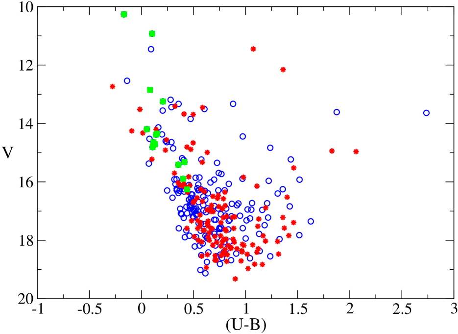
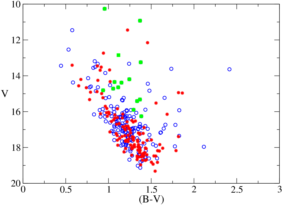
Figure 3: Left: $V$ magnitude against $(U-B)$ colour for the two frames observed in the region of Berkeley 90. Right: $V$ magnitude against $(B-V)$ colour for the two frames observed in the region of Berkeley 90. In both diagrams, blue open circles are stars observed in the field centred on the cluster; red stars are objects observed in the area to the southeast of Berkeley 90; and green filled squares are early-type stars spectroscopically observed.

3.2.2 Determination of the $R_{5495}$ value and a preliminary E(B-V)

The next step is to determine whether the extinction law in the direction of the cluster is standard. To this aim, we used the latest version of the software package CHORIZOS (Maíz Apellániz, 2004), with the stellar grid presented by Maíz Apellániz et al. (2013) for the 11 brightest OB main-sequence stars. CHORIZOS fits synthetic photometry derived from the spectral energy distribution of a stellar model convolved with an extinction law to reproduce the observed magnitudes. We used as input the $UBVRJHK_{\textrm{S}}$ photometry and the effective temperature, $T_{\textrm{eff}}$, corresponding to the spectral types (this calibration is an adapted version of Martins et al. (2005) which includes the spectral subtypes used by Sota et al. (2014). In fact, $T_{\textrm{eff}}$ was not fixed, but allowed to vary within small limits to improve the fit. The output of CHORIZOS is the monochromatic value of $R$ for each star, and its integrated colour excess and extinction, which are displayed in Table 3. We calculated then the individual value of $R_{V}$ for each star using the values of $A_{V}$ and $E(B-V)$. After excluding from the calculation star 47 (because its value for $R$ deviates by more than 1-$\sigma$ from the median value), we obtain a final median value of $R_{V}=3.51\pm 0.07$ which we will be using in the following analysis.

Table 3: Parameters obtained for 13 bright stars in the cluster using the CHORIZOS code.

Name	$\chi^{2}_{\textrm{red}}$	$T_{\textrm{eff}}$(K)	LC	$E(4405-5495)$	$R_{5495}$	$\log\,d$ (pc)	$A_{V}$	$E(B-V)$
36	1.325	34900	5	$1.668\pm 0.014$	$3.334\pm 0.037$	$3.355\pm 0.003$	$5.580\pm 0.025$	$1.646\pm 0.013$
47	0.707	22000	5	$1.282\pm 0.014$	$3.890\pm 0.065$	$3.373\pm 0.008$	$5.010\pm 0.045$	$1.267\pm 0.013$
57	3.650	32500	5	$1.496\pm 0.013$	$3.468\pm 0.041$	$3.569\pm 0.003$	$5.213\pm 0.025$	$1.480\pm 0.013$
59	2.600	22000	5	$1.268\pm 0.014$	$3.491\pm 0.050$	$3.556\pm 0.004$	$4.454\pm 0.026$	$1.252\pm 0.013$
67	1.617	22000	5	$1.552\pm 0.014$	$3.321\pm 0.040$	$3.553\pm 0.004$	$5.174\pm 0.027$	$1.524\pm 0.013$
70	4.050	25400	5	$1.386\pm 0.013$	$3.439\pm 0.045$	$3.509\pm 0.004$	$4.793\pm 0.026$	$1.368\pm 0.013$
75	3.750	23700	5	$1.341\pm 0.013$	$3.381\pm 0.045$	$3.559\pm 0.003$	$4.561\pm 0.024$	$1.324\pm 0.013$
88	1.475	20000	5	$1.129\pm 0.013$	$3.483\pm 0.056$	$3.591\pm 0.004$	$3.960\pm 0.026$	$1.115\pm 0.013$
90	3.275	21700	5	$1.603\pm 0.014$	$3.544\pm 0.040$	$3.417\pm 0.003$	$5.696\pm 0.025$	$1.574\pm 0.013$
92	0.812	20000	5	$1.575\pm 0.036$	$3.509\pm 0.097$	$3.565\pm 0.007$	$5.537\pm 0.050$	$1.545\pm 0.034$
176	1.732	41900	4	$1.217\pm 0.013$	$3.515\pm 0.052$	$3.269\pm 0.003$	$4.311\pm 0.025$	$1.212\pm 0.013$
178	2.447	41300	1	$1.611\pm 0.013$	$3.473\pm 0.039$	$3.390\pm 0.004$	$5.612\pm 0.025$	$1.592\pm 0.013$
283	3.150	31300	5	$1.423\pm 0.013$	$3.194\pm 0.040$	$3.390\pm 0.003$	$4.574\pm 0.024$	$1.407\pm 0.012$

3.2.3 The reddening-free $Q$ parameter, photometric spectral types and reddening

The reddening-free $Q$ parameter allows a preliminary selection of early-type stars. The $Q$ parameter is defined as:

$$Q=(U-B)-\frac{E(U-B)}{E(B-V)}(B-V)\,.$$ (1)

The value of $E(U-B)/E(B-V)$ is $0.72$ for a standard reddening law (Johnson & Morgan, 1953). For higher accuracy in the reddening procedure, and given that the value of $R_{V}$ is higher than standard, we calculated the $E(U-B)$ and $E(B-V)$ values for all the stars in our data set with spectra and $UBV$ photometry, using the intrinsic colours from Fitzgerald (1970). We plotted the $E(U-B)/E(B-V)$ diagram for these stars and obtained the equation of the line that fits best those points using the linear least squares fitting technique. In this case, the value of the line’s slope calculated is $0.81$, and we used this value when we determined the value of $Q$ for all stars in the two fields. As all B-type stars have a negative $Q$ parameter, we selected only stars with $Q\leq 0$, corresponding to the early-type members of the cluster, and we assigned them photometric spectral types (Johnson & Morgan, 1953). Given our magnitude limits, we do not expect to have reached any cluster members with spectral types later than B-type. For a few stars, there is not a good match between their derived photometric spectral types and their position in the $V$/$(B-V)$ diagram. We consider these objects early-type non-members (two of them, 14 and 179, are spectroscopically confirmed in Table 1). We identify the rest of the objects (45) as likely members of the cluster (see Figure 4). We determined individual $E(B-V)$ values for all members, by finding their intrinsic colours. For this, we used the $(U-B)$/$(B-V)$ diagram to slide the stars along the reddening vector (with slope of 0.81) until reaching a position on the unreddened standard relation (Johnson & Morgan, 1953), from which we obtained their accurate intrinsic colour $(B-V)_{0}$. We list their values of $E(B-V)$, $(B-V)_{0}$, $V_{0}$ and photometric spectral types in Table 4.

The $E(B-V)$ values range from 1.0 until 1.6, with a median value of $1.4\pm 0.2$. Most stars have $E(B-V)$ values higher than 1.2 and we find most stars between 1.3 and 1.4 (10 and 11 stars, respectively). The spatial distribution of these values is shown in Figure 4. Open circles are members with $E(B-V)\leq 1.3$ and open squares are members with $E(B-V)>1.3$. The main conclusion is that the members located near the cluster core have higher values of the reddening.

We carried out the same analysis with stars located in the southeast frame. We found a sequence of 29 B-type stars which have spectral types consistent with their positions in the $V$/$(B-V)$ diagram. They correspond to a single early-type population located at the same distance as Berkeley 90. In Table 5, we list the values of $E(B-V)$, $(B-V)_{0}$, $V_{0}$ and photometric spectral types for all the stars considered members of this population. The $E(B-V)$ values range from 1.0 until 1.6 with a median value of $1.3\pm 0.2$, consistent with that of cluster members. Most stars have reddening between 1.3 and 1.4, but the difference with the members of Be 90 is that the lower values of reddening are more populated than the higher values. In Figure 4 we can also see the distribution of these values for components of that early-type sequence, using the same symbols as in the frame corresponding to Be 90. This result confirms again the higher reddening towards the cluster core.

Table 4: Values of $E(B-V)$, $(B-V)_{0}$, $V_{0}$ and photometric spectral types for likely B-type members in Berkeley 90.

Star	$E(B-V)$	$(B-V)_{0}$	$V_{0}$	Photometric
				spectral types
1	1.49	$-$0.02	13.37	B9
7	1.58	$-$0.18	11.37	B3
15	1.39	$-$0.18	11.37	B3
17	1.34	$-$0.17	11.50	B5
18	1.16	$-$0.13	12.05	B7
22	1.42	$-$0.14	12.00	B5
36	1.70	$-$0.32	7.29	O–B0
42	1.65	$-$0.17	11.51	B5
44	1.28	$-$0.07	12.86	B9
45	1.35	$-$0.19	11.35	B5
46	1.29	$-$0.15	11.75	B7
47	1.33	$-$0.26	9.69	B2
50	1.47	$-$0.16	11.73	B5
57	1.53	$-$0.29	8.81	O–B0
59	1.30	$-$0.25	10.15	B2
61	1.49	$-$0.23	10.69	B2
63	1.56	$-$0.19	11.22	B3
65	1.06	$-$0.13	12.13	B8
67	1.59	$-$0.25	9.85	B2
70	1.41	$-$0.26	9.43	B1
71	1.12	$-$0.10	12.68	B8
75	1.36	$-$0.25	9.86	B1
80	1.50	$-$0.21	11.03	B2
82	1.63	$-$0.15	11.84	B5
83	1.28	$-$0.11	12.44	B8
84	1.52	$-$0.23	10.55	B2
88	1.16	$-$0.22	10.75	B2
90	1.62	$-$0.26	9.63	B2
92	1.62	$-$0.24	10.58	B2
112	1.35	$-$0.13	12.16	B8
115	1.26	$-$0.17	12.02	B5
117	1.38	$-$0.11	12.44	B8
118	1.00	$-$0.09	12.78	B8
128	1.40	$-$0.12	12.25	B8
133	1.25	$-$0.13	12.12	B7
138	1.17	$-$0.13	12.16	B8
140	1.26	$-$0.25	10.09	B1
141	1.20	$-$0.12	12.23	B7
157	1.39	$-$0.20	11.18	B3
161	1.02	$-$0.12	12.34	B7
163	1.26	$-$0.11	12.42	B8
172	1.28	$-$0.12	12.30	B7
176	1.29	$-$0.33	5.75	O–B0
178	1.70	$-$0.33	4.96	O–B0
181	1.36	$-$0.12	12.28	B7

Table 5: Values of $E(B-V)$, $(B-V)_{0}$, $V_{0}$ and photometric spectral types for likely B-type members in Southeast Berkeley 90.

Star	$E(B-V)$	$(B-V)_{0}$	$V_{0}$	Photometric
				spectral types
185	1.23	$-$0.15	11.88	B5
188	1.32	$-$0.12	12.39	B7
191	0.96	$-$0.17	11.54	B5
206	1.39	$-$0.11	12.53	B8
210	1.11	$-$0.12	12.37	B8
217	1.12	$-$0.03	13.29	B9
219	1.37	$-$0.13	12.12	B8
220	1.29	$-$0.12	12.32	B8
222	1.26	$-$0.15	11.93	B7
224	1.37	$-$0.13	12.14	B7
232	1.35	$-$0.19	11.40	B3
236	1.27	$-$0.25	9.87	B1
237	1.24	$-$0.12	12.30	B7
238	1.25	$-$0.31	8.34	O–B0
239	1.18	$-$0.27	9.38	B1
250	1.11	$-$0.13	12.17	B7
254	1.12	$-$0.16	11.76	B5
255	1.33	$-$0.13	12.13	B7
260	1.38	$-$0.13	12.16	B7
265	1.45	$-$0.11	12.50	B8
268	1.14	$-$0.13	12.13	B7
269	1.12	$-$0.14	11.89	B7
271	1.38	$-$0.12	12.34	B8
278	1.31	$-$0.12	12.36	B7
283	1.44	$-$0.32	7.80	O–B0
291	1.62	$-$0.05	13.13	B9
295	1.49	$-$0.05	13.16	B9
297	1.65	$-$0.10	12.69	B8
301	1.98	$-$0.19	11.24	B5

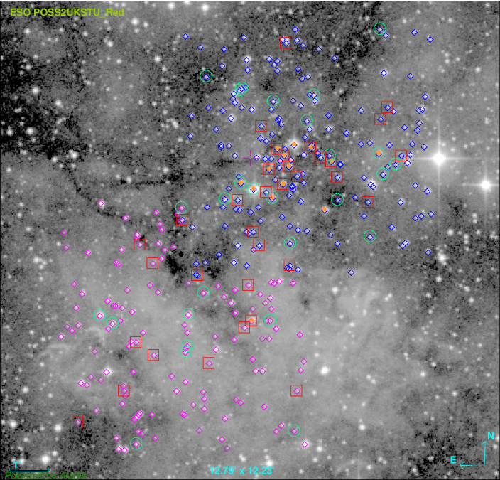
Figure 4: Stars with optical photometry in the frame corresponding to the open cluster Be 90 (blue open diamonds) and those of the southeast frame (pink open diamonds). Open big squares in red represent stars with a value of $E(B-V)$ higher than 1.3. Open big circles in green are stars with a value of $E(B-V)$ lower or equal to 1.3. Main-sequence stars with spectra are marked with filled small circles in orange. North is up and east is left. The size of the image is $12.79\arcmin\times 12.23\arcmin$. It is a DSS2 Red image.

3.2.4 Determination of distance and age

We plot the $M_{V}$/$(B-V)_{0}$ diagram for all members in the fields of Berkeley and southeast of Berkeley 90 (see Fig. 5). We use the observational ZAMS from Schmidt-Kaler (1982), shifted to different distance moduli, to determine a distance modulus (DM) to the cluster of $12.7\pm 0.3$, where we assume a relatively conservative error in the by-eye fit of $\pm 0.3$. This value corresponds to a distance of $3.5^{+0.5}_{-0.5}$ kpc. We can test this result by comparing the absolute magnitudes obtained in this diagram for each known spectral type to the values in the spectral type calibration by Turner (1980). All the B-type stars with photometric and spectroscopic spectral types match the calibration if its intrinsic dispersion (due not only to the finite size of the subtypes, but also to physical causes such as fast rotation, inclination to the line of sight and binarity) is taken into account. In contrast, O-type stars appear systematically too bright. Star 283 (O9.5 V) is more than half a magnitude too bright, while star 36 is almost one magnitude too bright. LS III $+46\degr$12 is also, as discussed at length in Paper I, much brighter than expected. Though we cannot offer an explanation with the current data, this excess brightness very likely points towards a high multiplicity in all the O-type stars. In the case of 36, we have to note that its H$\alpha$ photometry in the IPHAS catalogue (see figure 7 in Paper I and the corresponding discussion, where it is referred to as 2MASS J20350798+4649321), places it in a region typical of emission-line stars. There is no indication of such behaviour in our spectrum, while Oe stars of such an early spectral type are extremely rare in the Milky Way (Negueruela et al., 2004). Finally, we note that this distance for the cluster is compatible within their respective errors with the average of the distances obtained from the CHORIZOS analysis $d=3.0\pm 0.6$ kpc (the error here is the standard deviation).

Given that there are no evolved stars in the cluster (even the O3.5 If* supergiants are in all likelihood main sequence stars; see discussion in Paper I), we cannot fit any isochrone in the $M_{V}$/$(B-V)_{0}$ diagram to determine the age. We can only assert that the age of the cluster is less than 3 Ma, because we still have a full complement of O-type stars on the main-sequence. Stars considered members in the two frames form a single sequence, and so are located at the same distance. In the $(U-B)$/$V$ CMD (Fig. 3) we can see that the two populations fit very well to the ZAMS and form a single sequence of early-type stars, while in the $(B-V)$/$V$ CMD stars from the Southeast frame occupy positions consistent with lower reddening. Therefore this second population has an age similar to that of the cluster. In the next section, we analyse the relationship between these two populations.

Given its Galactic coordinates ($l=84\aas@@fstack{\circ}9$, $b=+3\aas@@fstack{\circ}8$) and its distance ( $d=3.5^{+0.5}_{-0.5}$ kpc), Berkeley 90 is very likely to be placed in the Perseus arm, which has tracers at $d\la 4$ kpc around $l=95\degree$ – $100\degree$ (Choi et al., 2014), as the Local arm does not seem to extend in this direction (Xu et al., 2013). Unfortunately, there are no other clusters catalogued in the area that could be used to constrain structure in this Galactic region. Other clusters with about same Galactic longitude ($\sim 85\degree$) have very different latitudes. We can cite Berkeley 88, NGC 7024, NGC 6996 and NGC 6989 (with $b=+6\aas@@fstack{\circ}5$, $b=-3\aas@@fstack{\circ}9$, $b=+0\aas@@fstack{\circ}1$ and $b=+0\aas@@fstack{\circ}3$, respectively), but there are no in-depth studies on any of them providing accurate properties yet.

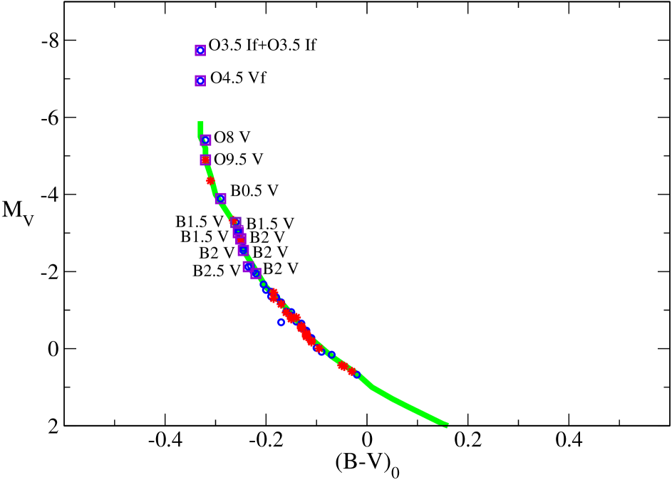
Figure 5: Absolute magnitude $M_{V}$ against intrinsic colour $(B-V)_{0}$ for Berkeley 90 and southeast of Berkeley 90. Blue open circles are stars observed in the field centred on the cluster. Red stars are objects observed in the area to the southeast of Berkeley 90. Open violet squares are early-type stars spectroscopically observed. The solid line represents the ZAMS from Schmidt-Kaler (1982).

3.2.5 Near-IR photometry

The centre and size of Berkeley 90 were set by Tadross (2008) using 2MASS data. This area, corresponding to a diameter of $5\arcmin$, was fully covered by our optical photometry (a $6\aas@@fstack{\prime}5\times 6\aas@@fstack{\prime}5$ frame). However, 2MASS data clearly suffer from incompleteness due to confusion near the cluster core, as many of our optically identified stars lack 2MASS counterparts. Therefore we used the near-IR photometry obtained from the UKIDSS images covering the same size as our optical images. First, we plot the $K_{\textrm{S}}$/$(J-K_{\textrm{S}})$ diagram for Berkeley 90 (see Fig. 6). We used the values of $E(B-V)$ and distance modulus obtained in Section 3.2.3 and Section 3.2.4 to draw the early-main sequence, ranging from spectral type M6 until B3, with $Z=0.02$ and no overshooting. The early main sequence is defined as the stellar locus at the time when the star settles on the main sequence after the CN cycle has reached its equilibrium, which only affects stars with a mass higher than $1.2\>$M_☉. We plot the pre-main sequence (PMS) isochrone of 3 Ma with the same parameters as well. Both tracks are taken from Siess et al. (2000).

We obtained a median value of $R_{V}=3.51\pm 0.07$ in Section 3.2.2 which deviates from the standard value of $R_{V}=3.1$ and, therefore, we cannot use the standard relationship between $E(B-V)$ and $E(J-K_{\textrm{S}})$. Using the extinction laws implemented in CHORIZOS, we determined the values of $E(J-K_{\textrm{S}})$ and $A_{K_{\textrm{S}}}$ that correspond to $E(B-V)\sim 1$, the lowest value measured for cluster members (see Table 4) when $R_{V}=3.51$ (finding $E(J-K_{\textrm{S}})=0.65$ and $A_{K_{\textrm{S}}}=0.44$) and displaced the main-sequence and PMS isochrone to these values. In Fig. 6, we use pink dots to represent all stars with near-IR photometry. The likely B-type members (from the optical analysis) are represented as black filled circles. There is a population of faint sources close to the main-sequence, but a much larger population around the 3 Ma isochrone, which is the estimated maximum age for the cluster. Taking this into account, we can interpret the pink dots with $(J-K_{\textrm{S}})\leq 1.2$ as foreground stars, while the rest of the stars are the PMS population of the cluster together with some field contamination that we estimate below.

To characterize the PMS stars, we carried out the same procedure as in Section 3.2.9 from Marco & Negueruela (2016), using WISE data and the near-IR $Q$ index. There are 146 stars with WISE counterparts in the field of Be 90, and 69 in the field of the southeast of Be 90. We used the $(K_{\textrm{S}}-W1)$ against $(W1-W2)$ and $(H-K_{\textrm{S}})$ against $(W1-W2)$ diagrams to classify the stars as either objects with disc or discless, following the criteria described in Koenig et al. (2012) and Koenig & Leisawitz (2014). We were not able to utilize diagrams based on the $W3$ or $W4$ bands, because dust emission from the molecular cloud dominates these bands for all sources in this area. To reach fainter stars, we can use the $(J-H)-(H-K_{\textrm{S}})$ diagram, or equivalently the IR $Q$ reddening-free index. Stars with discs or strong infrared excess have negative values of $Q$ (Negueruela & Schurch, 2007) and we take $Q\leq-0.1$ as the condition to identify such stars.

In Fig. 6, stars identified as discless from the WISE photometry are marked with the blue pluses. Most of them match with B-type main-sequence stars or obvious non-members. PMS stars with disks are represented by the green filled squares. Stars with $Q\leq-0.1$ are the brown crosses. These two populations represent the PMS population living in the cluster. They are placed on the right side of the diagram because they have an excess in the $(J-K_{\textrm{S}})$ colour arising from the disk. As WISE photometry is relatively shallow, we only find systems with disks among the brightest targets (down to $K_{\textrm{S}}\approx 15$ mag). The green squares with $K_{\textrm{S}}\la 14$ mag likely correspond to the massive PMS stars ($M\geq 3M_{\sun}$), while the brown crosses extend to fainter magnitudes, covering the same range of $(J-K_{\textrm{S}})$. We interpret them as lower-mass PMS objects. To estimate the level of contamination by background stars, we plot the approximate position for red clump stars at the distance and reddening of the cluster as a big open square. We can project this locus along the reddening vector (drawn on the top of the figure) to see their possible positions in the diagram. We do not find many objects compatible with these locations, and most of them have characteristics that identify them as PMS stars. Indeed, if we select stars with $Q\ga 0.35$ (typical of red giants), we find that most of them have $K_{\textrm{S}}$ magnitudes in the range 16 – 17 and, therefore, cannot be red giants, because they are very far away from their possible positions. They must then be foreground red dwarfs. The low contamination by background red giants is not surprising, given the moderately large distance to the cluster and its height above the Galactic plane.

Furthermore, we plot in Fig. 6 the $K_{\textrm{S}}$/$(J-K_{\textrm{S}})$ diagram for the southeast of Berkeley 90 as well. We took the near-IR photometry from the UKIDSS images covering the same area as our optical frames. We use the same values of the parameters as for Berkeley 90 to build the diagram. The symbols represent the same kinds of objects as in the Berkeley 90 diagram. We can also see a PMS population living in this area, associated with the stars considered members based on the optical photometry. In fact, the distribution of sources in this CMD is very similar to that found in the CMD for the cluster.

We represent the spatial distribution of the PMS stars in the two regions studied in Fig. 7. We plot the stars classified as PMS stars with discs from WISE data as white circles; the rest of the PMS low-mass population, surrounding these stars in the $K_{\textrm{S}}$/$(J-K_{\textrm{S}})$ diagram, as blue squares (in this map, we are using only stars with $(J-K_{\textrm{S}})\geq 1.5$ and $K_{\textrm{S}}\leq 16$ to avoid the noise caused by objects with low-precision photometry). We can see that both kinds of PMS objects are detected in the cluster frame, but the low-mass population is not seen in the lower part of the southeast frame. All the objects from its $K_{\textrm{S}}$/$(J-K_{\textrm{S}})$ diagram fulfilling $(J-K_{\textrm{S}})\geq 1.5$ and $K_{\textrm{S}}\leq 16$ (i.e. low-mass PMS candidates) are concentrated near the border line with the Be 90 frame (to the North). The WISE image shows that the area where we do not detect low-mass PMS stars has a much higher amount of thick dust that appears projected in front of the population. This suggests two possible (non-exclusive) explanations for the detection of only WISE candidates to intermediate-mass PMS stars in this part of the frame. On the one hand, the population may still be embedded, with only the brightest, most massive PMS stars being detectable. On the other hand, the population in this area could be younger than the cluster, with the low-mass stars still being formed. Since we are not able to determine the age of the cluster, but an age of 2 – 3 Ma is probable (see also the discussion in Paper I, ), there is some room for an age spread, implying sequential, perhaps triggered, star formation to the South of the cluster. Some support for this hypothesis comes from the detection in this area of a very massive PMS star. This object, which can be seen in Fig. 6 (right-hand panel) as the brightest early-type star in $K_{\textrm{S}}$, is star 238, whose colours identify it as a very early star. A red spectrum is displayed in Fig. 8, showing H$\alpha$ and He i 6678 Å in emission. Its blue spectrum shows that it is a Herbig Be star with spectral type between B0.5 and B1. This is necessarily a very young object.

In view of this, we can speculate that star formation is still occurring close to the bright illuminated rims to the south of our field, where at least one “elephant-trunk” structure can be seen in the DSS2 images close to star 238 (see also Fig. 7 where 238 is the easternmost star with disc). There is no measurable age difference between the core of the cluster and the area immediately south of it (i.e. the top half of our southwest frame), but there does seem to be a difference with respect to the region rich in gas and dust, as only massive PMS stars can be seen in the mid-IR in this region. So, we conclude that there is some evidence for sequential star formation in this area. The population to the south of the cluster has the typical characteristics generally associated with triggered star formation (even though we have no obvious evidence for triggering here beyond the age difference): a smaller population (we observe the presence of less main-sequence and pre-main-sequence stars) and an absence of the most massive stars (there is only an O9.5 V star in the region immediately south, and only early-B stars in the region still rich in dust, against the early-O stars in the cluster).

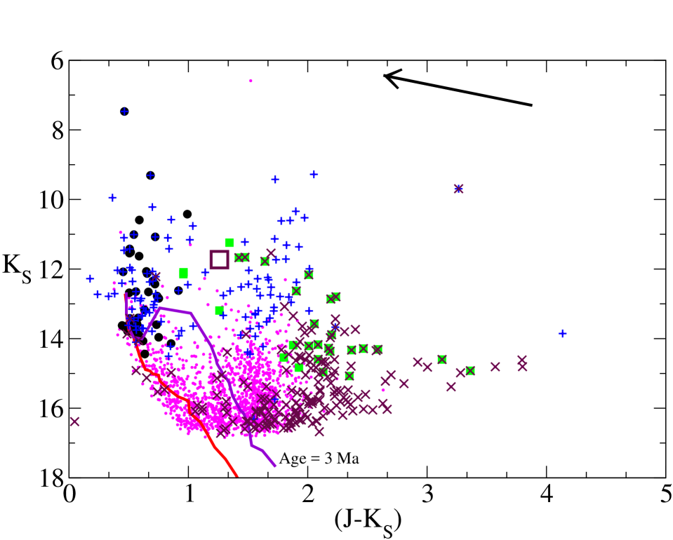
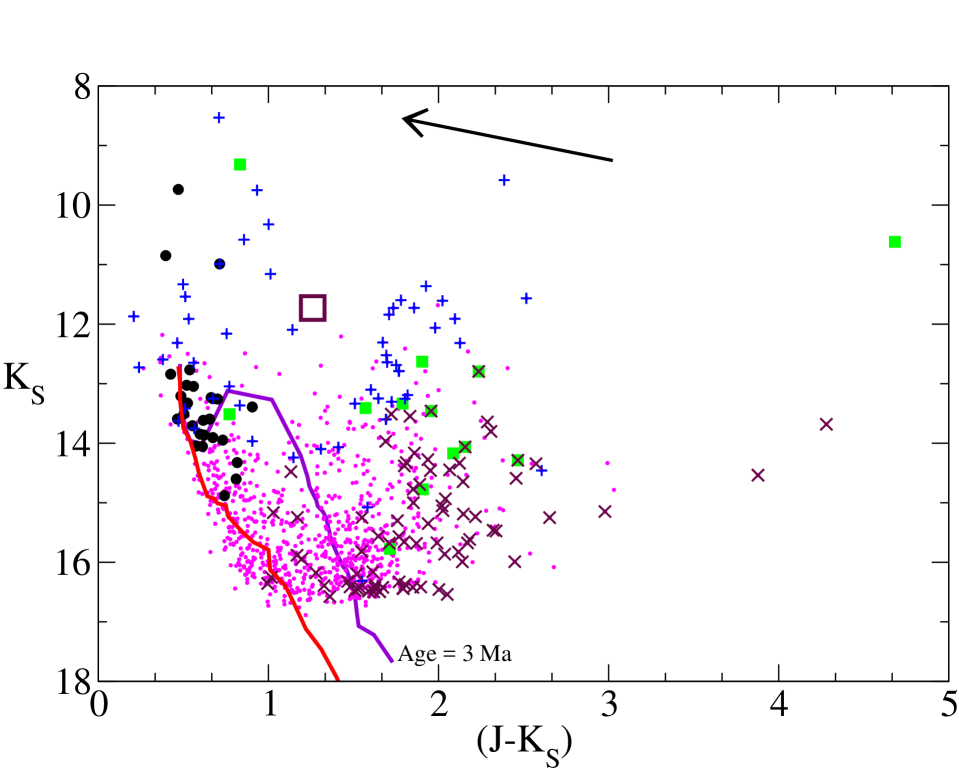
Figure 6: Left: $K_{\textrm{S}}$ magnitude against $(J-K_{\textrm{S}})$ colour for Berkeley 90. Right: $K_{\textrm{S}}$ magnitude against $(J-K_{\textrm{S}})$ colour for the area of southeast Berkeley 90. We use pink dots to represent all stars with near-IR photometry. The likely B-type members (from the optical analysis) are represented as the black filled circles. Stars identified as discless from the WISE photometry are marked with the blue pluses. PMS stars with discs according to the WISE criteria are represented by green filled squares. Stars with $Q\leq-0.1$ are the brown crosses. The big open square indicates the approximate position for red clump stars at the distance and reddening of the cluster. The red line is the early main sequence and the purple line is the 3 Ma PMS isochrone, both taken from Siess et al. (2000). The reddening vector $K_{\textrm{S}}=0.68\cdot(J-K_{\textrm{S}})$ of length 1.5 mag is indicated by the arrow. See text for further details.

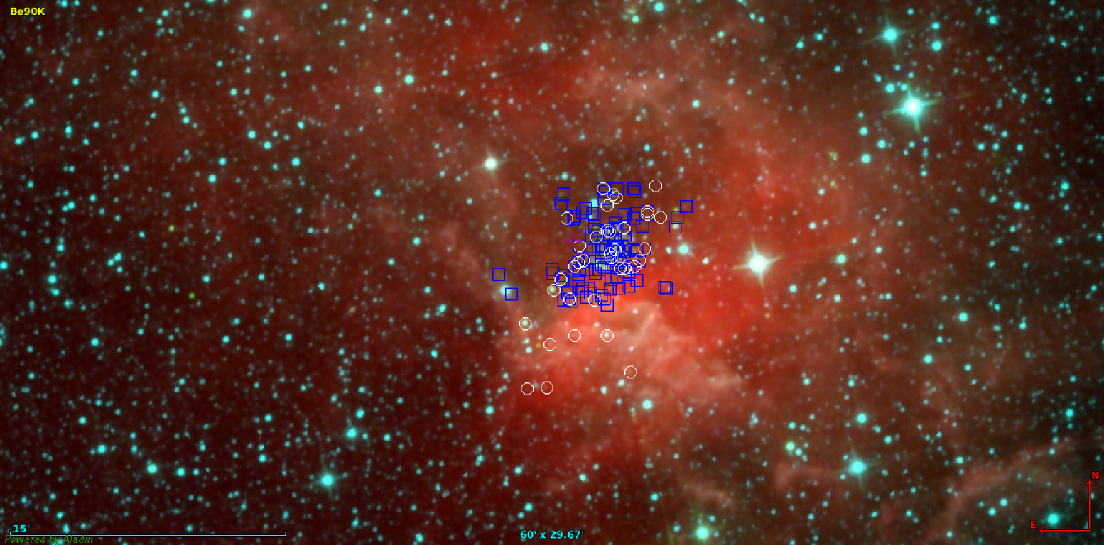
Figure 7: Spatial distribution of the PMS stars in the two areas studied. The image, downloaded from Aladin, is provided by the WISE mission. The filters $W1$, $W2$ and $W4$ are represented by blue, green and red, respectively. White circles represent stars with discs. Blue squares are low mass stars selected with the infrared $Q$ index and occupying the same location in the $K_{\textrm{S}}$/ $(J-K_{\textrm{S}})$ diagram that the stars with discs but reaching fainter $K_{\textrm{S}}$ magnitudes. The Herbig Be star (S238) is the easternmost star with disc, to the southeast of the cluster (clearly recognizable by the high concentration of PMS stars), on the bright dust shell. North is up and east is left. The size of the image is $1\degree\times 29.67\arcmin$.

Figure 8: Intermediate-resolution spectrum of star 238 around H$\alpha$ showing emission lines typical of an early-type Be star. The equivalent width of H$\alpha$ is $-45\,$Å.

4 Discussion

4.1 Cluster mass

One of the most important issues in modern astrophysics is the determination of the IMF with which a group of stars is formed. We carry out this work in the open cluster Be 90. We have determined the upper-main-sequence population with accuracy using photometry and spectroscopy. We know how many stars there are between the different spectral ranges from O-type until B9-type stars. We can assign the stellar masses for each one using the calibrations from Harmanec (1988) and Martins et al. (2005) (see Table 6). The masses of the two components of LS III $+46\degr$11 are not known. The orbital solution only provides minimum masses of 39 and $36\>$M_☉ if we were seeing the system exactly edge on. We will assume conservative values of $50\>$M_☉, even though some studies suggest higher masses for this spectral type (e.g. Massey et al., 2005).

Table 6: Values of spectral types for early-type members and their mass from Harmanec (1988) and Martins et al. (2005), number of stars in the cluster, and total mass for each spectral type in Berkeley 90.

Spectral type	Mass ($M_{\sun}$)	Number	Total mass ($M_{\sun}$)
O3.5 If∗	50	2	100
O4.5 V(f)	42	1	42
O8.5 V	20.8	1	21
B0 V	14.6	0	0
B0.5 V	13.2	1	13
B1 V	11.0	1	11
B1.5 V	10.0	3	30
B2 V	8.6	7	63
B2.5 V	7.3	1	7
B3 V	6.07	4	24
B5 V	4.36	7	28
B7 V	3.38	7	21
B8 V	2.91	9	27
B9 V	2.52	2	6

Given our magnitude limit, the cluster parameters, and the range of $E(B-V)$ found in the cluster, we can only be sure that we are complete until spectral type B7. The IMF for stars more massive than the Sun in the Solar neighbourhood was determined by Salpeter (1955):

$$\xi(M)=\xi_{0}M^{-2.35}$$ (2)

where $\xi_{0}$ is the constant which sets the local stellar density. In our case, taking the Salpeter law, we can determine the number of stars ($N$) that form with masses between $M_{1}$ and $M_{2}$, by integrating the IMF between these limits:

$$N=\int_{M_{1}}^{M_{2}}\xi(M)dM=\xi_{0}\int_{M_{1}}^{M_{2}}M^{-2.35}dM\\ =\frac{\xi_{0}}{1.35}[M_{1}^{-1.35}-M_{2}^{-1.35}]$$ (3)

First, we needed to estimate the value of $\xi_{0}$. For that, initially we chose a box from B2 until B7 (from $9\>$M_☉ until $3\>$M_☉) where there are 26 stars and we are certain of completeness. We obtained a value of $\xi_{0}\approx 200$. Choosing a box between B0 and B2, where there are 12 stars and we are complete as well, the value that we get for $\xi_{0}$ is about 470. We have two different values for the same constant, using the distribution of the population of Be 90. Clearly, if we use these two values of $\xi_{0}$ to calculate the number of stars between $50\>$M_☉ and $1\>$M_☉, we will obtain two different results. In principle, we should have the same value for the constant, using the number of stars from whatever size of box where we are counting all stars belonging to the box. The obvious conclusion is that, with such poor sampling of the upper-IMF, the size of the box one chooses may determine the results. Statistical fluctuations in the upper-main-sequence may affect the calculation of $\xi_{0}$.

With this information in mind, we decided to estimate the total mass of the cluster using the value of the constant $\xi_{0}$ provided by the box covering the [B2-B7] range, because it contains more stars and the mass range is better constrained. The total mass in stars born with mass $M_{1}=50\>$M${}_{\sun}\geq M\geq M_{2}=1\>$M_☉ should be:

$$M=\int_{1M_{\sun}}^{50M_{\sun}}M\xi(M)dM\\ =\xi_{0}\int_{M_{1}}^{M_{2}}M^{-1.35}dM=427M_{\sun}\\$$ (4)

This result is the mass of the cluster down to solar-type stars. To estimate the low-mass component, we can use the Kroupa & Bouvier (2003) standard IMF, for which the total mass of the cluster should be around twice this value. This means that Berkeley 90 is an intermediate-mass cluster with a total mass close to, but below, 1000 M_☉ which still contains three very massive stars in the upper-main sequence. We can see in Table 6 that the sum of the total mass in early-type stars is 393 M_☉. But, if we ignore these three most massive stars (contributing around 150 M_☉), we are left with only $240\>$M_☉, which is more compatible with the standard IMF and the estimated total mass of the cluster (about one third of the total mass). Again, we see how our calculations are dominated by very small number statistics and thus trying to calculate an observational slope for the IMF in Berkeley 90 would not make sense. Moreover, this estimate does not take into account the effect of binarity, which would take the mass of the cluster slightly above $1\,000\>$M_☉.

In figure 1 from Weidner et al. (2010) we can see different relationships between the mass cluster and the mass of the most massive star in the cluster. In this case, the value for Be 90 ($\log\,M_{\textrm{cl}}\la 3$, $\log\,M_{\textrm{max}}\ga 1.7$) is above all relations, but not far from the values given by Oey et al. (2005, short-dashed-long-dashed line in their figure) or Elmegreen (2000, short-dashed line). It may be argued that, in order to have a fair comparison with other clusters in the literature, the population to the southeast of Be 90 should also be taken into account. However, given the number of stars detected, this region could add at most 50% to the total mass, still leaving the total population of the region around $1\,500\>$M_☉, and not changing the conclusions in any substantial way.

4.2 A search for runaway stars

A high fraction of the O-type field stars (22/43) can be considered to be runaway star candidates, based on their present or former peculiar space velocity, and the vicinity of some of them to very young clusters ($\leq 10$ Ma) (de Wit et al., 2005). This is expected, because $N$-body simulations of massive clusters predict that the fraction of stars expelled by dynamical processes from the clusters may be as high as (20-25)% of O-type stars and (10-15)% of early-B type stars (Fujii & Portegies Zwart, 2011; Oh & Kroupa, 2016).

Be 90 is not considered a massive cluster in the Milky Way because its mass is very far away from the minimum value of $10\,000\>$M_☉. However, it is not only the home of the one of the most massive systems in the Galaxy (LS III $+46\degr$11), but also contains at least one other early-O massive star. In contrast, its population of late-O and early-B (B0 – B2) stars is scarce (only 12 stars). This distribution of stars is unusual. There are other similar cases (e.g. Negueruela & Marco, 2008), but it is not very common. Even though the ejection of $\sim 20$% of the massive stars would not seriously affect the conclusions with respect to the relation between the cluster mass and the most massive member, it would make the observed IMF still more top-heavy, favouring even more the idea of random sampling.

We know that the highest possible velocity of dynamical ejection is $\sim 100\>\textrm{km}\,\textrm{s}^{-1}$, with values of 10 – $20\>\textrm{km}\,\textrm{s}^{-1}$ being more typical of this scenario. In the extreme case, a runaway star could travel 1 pc in 10 000 yr, while for a typical case, 50 000 yr would be required. Be 90 is located at a distance of $3.5^{+0.5}_{-0.5}$ kpc and its maximum possible age is about 3 Ma. So, considering the upper limit on age of 3 Ma, the distance travelled is 300 pc for the first case and 30 pc for the typical case. At the distance of the cluster, 300 pc are equivalent to $\sim 5\degree$, while 30 pc are $\sim 0.5\degree$. While any search over the larger radius would be impractical, the smaller distance is comparable to the apparent size of Sh2-115 in the sky. We have searched for candidate runaway O-type stars in this region, using archival data and the techniques outlined in Negueruela & Schurch (2007).

Initially, we selected all stars in 2MASS with good quality flags and photometric errors $<0.04$ mag in all bands and then plotted the $K_{\textrm{S}}$/$Q_{\textrm{IR}}$ diagram. Early-type stars form a well-defined vertical sequence between $Q\approx-0.05$ and $0.05$. We selected stars in this range with $K_{\textrm{S}}$ magnitudes brighter than 11.0, i.e. fainter than any O-type star in Be 90. The vast majority of these objects have $(J-K_{\textrm{S}})<0.2$, indicative of very low reddening and are obviously foreground to the cluster. Many of them are already catalogued as late-B stars, such as HD 196832 or BD $+46\degr$2968. An interesting case is BD $+46\degr$2978, but Crampton & Fisher (1974) classify it as B0 III (i.e. an evolved star) and place it closer to us than the cluster. The same authors classify BD $+46\degr$2972 as O9.5 V placing it at a distance of 3.4 kpc. Even though these parameters suggest a connection to Sh2-115, inspection of the 2MASS images shows that this is really a multiple system with at least two early-type stars, ruling it out as a candidate runaway.

We find a small number of objects with $(J-K_{\textrm{S}})>2$ and $K_{\textrm{S}}$ brighter than any O-type star in the cluster. These objects are in all likelihood cool stars with dusty envelopes, whose S.E.D. reproduces that of reddened early-type stars (Comerón et al., 2002). Indeed, one of them is a catalogued Carbon star, CGCS 4916. We confirmed this possibility by checking their WISE colours. In all cases $(W1-W2)$ is positive and much higher than the value $\approx 0.0$ expected for early-type stars. We are finally left with a small number of candidates at low $(J-K_{\textrm{S}})\approx 0.3$ and four further candidates with $(J-K_{\textrm{S}})$ slightly higher than cluster members. We used the APASS catalogue to obtain the $B$ and $V$ magnitudes for these objects. A few of them, such as TYC 3573-1518-1, are so bright ($V\sim 10$) that they should be listed in the LS catalogue if they were OB stars. In addition, for example, TYC 3573-2322-1 has Tycho proper motions, and its projected motion is towards the cluster. In the end, there are only five stars that we cannot rule out as OB stars and candidate runaways, and we list them in Table 7. Given their magnitudes and colours, none of them can be earlier than an O9 – B0 star at the distance of the cluster. We find no candidate for an earlier-type runaway. This suggests that the number of ejections has been very low, as expected for the low mass of the cluster.

Table 7: Stars within $30\arcmin$ of Be 90 whose colours and magnitudes are compatible with OB stars at the cluster distance. $B$ and $V$ magnitudes are from APASS, while infrared magnitudes are from 2MASS.

2MASS	Other	$B$	$V$	$J$	$H$	$K_{\textrm{S}}$
20351892+4632438	TYC 3573-1354-1	12.5	11.8	10.40	10.17	10.06
20364196+4642428	TYC 3573-1558-1	12.1	11.4	10.07	9.85	9.74
20355132+4700204	$-$	15.8	14.2	10.61	10.15	9.89
20365851+4710569	$-$	15.2	13.8	10.73	10.29	10.08
20343597+4719192	$-$	14.6	13.5	10.66	10.25	10.02

4.3 The environment of O3-type stars in the Galaxy

The most massive stars are found almost exclusively in the most massive very young clusters, such as R136, the nuclear cluster of 30 Dor in the LMC. While the highest stellar masses measured correspond to WNh stars, such as NGC 3603 A1 (Schnurr et al., 2008), O2 – O3 stars represent the most massive stars with absorption-line spectra (Walborn et al., 2002), with masses above $40\>$M_☉ (Massey et al., 2005). In general, these objects are found only in the most massive Galactic clusters and associations, such as NGC 3603, Cyg OB2 or the Carina Nebula.

In the Galactic O star catalogue, we have found information about all catalogued O-type stars in the Milky Way earlier than O4 and the environments where they are living. We have a number of $\sim 20$ such stars, with many being binary or multiple systems. The places where we find this type of stars are as follows:

• The Carinae Nebula (NGC 3372) is the largest nebula in the southern sky. More than 60 O-type stars and several young open clusters are located in or near the nebula, including Trumpler 14 and Trumpler 16 in the bright part of the nebula. These clusters contain a number of O3.5 V stars, testimony to their extreme youth (Hur et al., 2012).

• NGC 3603 is the closest known giant H ii region. Its dense stellar core is populated by a large sample of O-type stars, including some very massive WNh stars and a number of O2 – 3 stars (Melena et al., 2008).

• NGC 6357 is a complex composed of giant molecular clouds, H ii regions and open clusters interacting with the parental gas, bubble-like structures and pillars, located around $l\sim 353\degree$, at a distance of 1.7 kpc. The young open cluster Pismis 24 is the most prominent of the stellar groups in the complex. Its population is formed by a number of coeval O-type stars, with the two brightest displaying spectral O3.5 I(f) and O3.5 III(f). Massi et al. (2015) estimate a cluster mass for Pismis 24 between $2\,000$M_☉ and $6\,000$M_☉, and conclude that there are indications of an early ejection of massive stars from the core of Pismis 24, suggesting a dynamically unstable environment after gas expulsion.

• The dispersed but very massive OB associations Cygnus OB2 contains two O3 If^∗ supergiants. These two stars appear younger and more massive than the bulk of the association, which presents a main-sequence turn-off at O6 V (Negueruela et al., 2008).

• Finally, two stars belong to small clusters: the ionizing star of Sh 2-158 in NGC 7538 (Maíz Apellániz et al., 2016) and HD 150 136 AaAb, the brightest components of the central star in NGC 6193. Two other stars lie within star forming regions, but not in clusters: HD 64568, classified as O3 V((f*))z and lying in relative isolation in the vicinity of the moderate-size star-forming region NGC 2467, far away from any of the open clusters catalogued in this region; and the primary in Bajamar star, O3.5 III((f*)), the ionizing star of the North America Nebula (Maíz Apellániz et al., 2016).

We can therefore see that about three quarters of stars earlier than O4 are associated with massive young clusters, while the remaining objects are part of intermediate mass clusters or star-forming regions. In the case of Be 90 we have one certain and one possible early-O binary systems without a large massive population. These cases of intermediate mass population provide some circumstantial evidence for random sampling of the IMF.

5 Conclusions

We have carried out a comprehensive photometric and spectroscopic study of the very young open cluster Berkeley 90, host to one of the most massive stellar systems in the Milky Way, LS III $+46\degr$11. Be 90 is a small, compact cluster (with a radius slightly above $2\arcmin$) that lies within the H ii region Sh2-115, occupying a small part of a cavity that is almost $30\arcmin$ across. Exploration of the cavity with 2MASS data reveals that, outside the cluster, there is only a sizeable young population immediately to the southeast of the cluster, towards a region characterized by bright illuminated rims and an ”elephant trunk” structure. We have presented optical, near and mid-IR photometry for a frame centred on the cluster and a partially overlapping frame that covers this region to the southeast.

We detect a sequence of 45 early-type stars in the cluster area with variable colour excess, between $E(B-V)=1.0$ and 1.6, with the higher values concentrating towards the cluster core. In the region to the southeast, we detect a similar sequence with very similar parameters, but a preference for the lower values of $E(B-V)$, comprising 29 stars, most of them of late-B spectral type (more easily reachable because of the lower reddening). From the analysis of the SED of stars with spectroscopy, we find a value of $R_{V}=3.5$, not unexpected in this region of the sky. Fitting of the ZAMS results in a distance of $3.5\pm 0.5$ kpc. The age of the cluster is not measurable, but different arguments suggest it is between 2 and $3\>$Ma.

Apart from the two catalogued early-O systems, we only find two other O-type stars in the region, an O8 V in the halo of the cluster and a O9.5 V towards the south. Estimation of a mass function is hindered by the very low number of objects in the upper bins and our incompleteness beyond spectral type B7, at least in the central area. We estimate a lower limit on the mass of the cluster of about $800\>$M_☉ for the standard IMF. Inclusion of the population to the southeast and a rough correction for binarity could put the total mass up to about $1\,500\>$M_☉. This is a low mass for a cluster containing stars of $\ga 50\>$M_☉, suggesting that random sampling and statistical fluctuations are very important at determining the mass of the most massive star in (at least, some) clusters.

Analysis of the near- and mid-IR photometry reveals a population of PMS stars associated with the cluster and immediately to its south. Further to the southeast, where there are signs of ongoing star formation, we identify a very early Herbig Be star, and a population of massive PMS stars in the vicinity of the gas and dust dark clouds. This represents evidence for sequential star formation, perhaps triggered by the very massive stars in the cluster.

Appendix A Photometric Tables

Table 8: Coordinates in J2000 and UBVR photometry for all stars in the field of Berkeley 90. Material on-line

RA(J2000)	DEC(J2000)	Star	$V$	$\sigma_{V}$	$(B-V)$	$\sigma_{B-V}$	$(U-B)$	$\sigma_{(U-B)}$	$(V-R)$	$\sigma_{(V-R)}$	N
20:35:26.97	$+$46:47:52.3	1	18.615	0.021	1.473	0.030	1.042	0.062	0.958	0.029	1
20:35:27.14	$+$46:47:53.7	2	19.130	0.033	1.372	0.042	0.614	0.061	0.941	0.046	1
20:35:03.96	$+$46:47:57.2	3	16.796	0.024	1.096	0.026	0.463	0.014	0.655	0.029	3
20:35:11.87	$+$46:48:02.0	4	15.349	0.019	1.159	0.020	0.726	0.009	0.655	0.022	6
20:35:13.26	$+$46:48:03.1	5	15.192	0.017	1.008	0.018	0.390	0.009	0.610	0.020	6
20:35:13.58	$+$46:48:03.9	6	17.931	0.014	1.380	0.019	0.632	0.030	0.837	0.023	3
20:35:13.06	$+$46:48:07.0	7	16.912	0.018	1.398	0.020	0.526	0.017	0.903	0.022	6
20:35:19.58	$+$46:48:07.2	8	17.613	0.012	1.352	0.015	0.759	0.023	0.865	0.019	4
20:35:27.09	$+$46:48:10.3	9	18.812	0.024	1.375	0.030	0.754	0.058	0.933	0.035	1

Table 9: Coordinates in J2000 and near-IR photometry for stars in the field of Berkeley 90. Material on-line

RA(J2000)	DEC(J2000)	$J$	$\sigma_{J}$	$H$	$\sigma_{H}$	$K_{S}$	$\sigma_{K_{S}}$
20:35:10.51	$+$46:48:55.3	17.527	0.037	15.983	0.020	15.560	0.034
20:35:12.30	$+$46:52:16.3	17.961	0.045	16.570	0.024	16.230	0.047
20:35:12.91	$+$46:50:31.2	18.208	0.043	16.759	0.025	16.362	0.052
20:35:28.20	$+$46:55:50.9	17.757	0.026	16.801	0.033	16.622	0.039
20:35:09.12	$+$46:50:43.6	16.722	0.049	15.962	0.054	15.875	0.053
20:35:31.02	$+$46:54:47.7	16.739	0.037	16.023	0.027	15.951	0.036
20:35:40.14	$+$46:53:46.5	17.392	0.048	16.427	0.025	16.208	0.031
20:35:17.64	$+$46:49:38.3	17.493	0.046	16.115	0.022	15.666	0.031
20:35:43.75	$+$46:55:53.4	17.295	0.043	16.491	0.037	16.358	0.056
20:35:05.22	$+$46:48:14.3	17.625	0.039	16.762	0.025	16.593	0.042
20:35:45.18	$+$46:55:23.3	16.822	0.024	16.019	0.037	15.871	0.029
20:35:42.63	$+$46:49:54.1	17.739	0.049	16.846	0.041	16.646	0.050
20:35:38.41	$+$46:54:46.5	17.228	0.040	16.450	0.030	16.313	0.042
20:35:49.67	$+$46:55:13.8	17.902	0.039	16.802	0.039	16.484	0.057
20:35:15.89	$+$46:52:06.8	16.903	0.033	16.139	0.027	16.004	0.038
20:35:56.08	$+$46:55:50.4	16.503	0.043	15.736	0.030	15.595	0.039
20:35:27.33	$+$46:49:15.4	17.461	0.038	16.659	0.024	16.496	0.046
20:35:57.90	$+$46:55:55.2	17.122	0.035	16.386	0.048	16.257	0.038
20:35:02.95	$+$46:48:14.2	17.292	0.035	16.435	0.020	16.237	0.042
20:35:32.23	$+$46:55:55.4	17.115	0.026	16.365	0.022	16.225	0.038
20:35:15.87	$+$46:55:39.7	17.517	0.037	16.681	0.032	16.490	0.028

References

- Beltrán & de Wit (2016) Beltrán, M. T., & de Wit, W. J. 2016, A&ARv, 24, 6
- Bonnell & Bate (2006) Bonnell, I. A., & Bate, M. R. 2006, MNRAS, 370, 488
- Casali et al. (2007) Casali, M., Adamson, A., Alves de Oliveira, C., Almaini, O., Burch, K., Chuter, T., Elliot, J., Folger, M., et al. 2007, A&A, 467, 777
- Choi et al. (2014) Choi, Y.K., Hachisuka, K., Reid, M.J., et al. 2014, ApJ, 790, 99
- Comerón et al. (2002) Comerón, F., Pasquali, A., Rodighiero, G., et al. 2002, A&A, 389, 874
- Crampton & Fisher (1974) Crampton, D., & Fisher, W.A. 1974, Publ. Dom. Astrophys. Obs. Victoria BC, 14, 283
- de Wit et al. (2004) de Wit, W. J., Testi, L., Palla, F., Vanzi, L., & Zinnecker, H. 2004, A&A, 425, 937
- de Wit et al. (2005) de Wit W.J., Testi, L., Palla, F. & Zinnecker, H. 2005, A&A 437, 247
- Elmegreen (1983) Elmegreen, B.G. 1983, MNRAS, 203, 1011
- Elmegreen (2000) Elmegreen, B.G. 2000, ApJ, 539, 342
- Fitzgerald (1970) Fitzgerald, M. P. 1970, A&A, 4, 234
- Fujii & Portegies Zwart (2011) Fujii, M. S., & Portegies Zwart, S. 2011, Science, 334, 1380
- Hambly et al. (2008) Hambly, N. C., Collins, R. S., Cross, N. J. G., Mann, R. G., Read, M. A., Sutorius, E. T. W., Bond, I., et al. 2008, MNRAS, 384, 637
- Harmanec (1988) Harmanec, P. 1988, Bull. Astron. Inst. Czech., 39, 329
- Hewett et al. (2006) Hewett, P. C., Warren, S. J., Leggett, S. K., Hodgkin, S. T. 2006, MNRAS, 367, 454
- Hodgkin et al. (2009) Hodgkin, S. T.; Irwin, M. J.; Hewett, P. C.; Warren, S. J. 2009, MNRAS, 394, 675
- Hur et al. (2012) Hur, H., Sung, H. & Bessell, M.S. 2012, AJ, 143, 41
- Johnson & Morgan (1953) Johnson, H.L., & Morgan, W.W. 1953, ApJ, 117, 313
- Koenig et al. (2012) Koenig, X. P., Leisawitz, D.T., Benford, D.J., et al. 2012, ApJ 744, 130
- Koenig & Leisawitz (2014) Koenig, X. P., Leisawitz, D. T. 2014, ApJ, 791, 131
- Kroupa & Bouvier (2003) Kroupa, P. & Bouvier, J. 2003, MNRAS, 346, 343
- Krumholz et al. (2009) Krumholz, M. R., Klein, R. I., McKee, C. F., Offner, S. S. R., & Cunningham, A. J. 2009, Science, 323, 754
- Lamb et al. (2010) Lamb, J.B., Oey, M.S., Werk, J.K, & Ingleby, L.D. 2010, ApJ, 725, 1886
- Landolt (1992) Landolt, A.U. 1992, AJ, 104, 340
- Larson (1995) Larson, R.B. 1982, MNRAS, 200, 159
- Larson (1995) Larson, R.B. 1995, MNRAS, 272, 213
- Lawrence et al. (2007) Lawrence, A., Warren, S. J., Almaini, O., Edge, A. C., Hambly, N. C., Jameson, R. F., et al. 2007, MNRAS, 379, 1599
- Maíz Apellániz (2004) Maíz Apellániz, J. 2004, PASP, 116, 859
- Maíz Apellániz et al. (2013) Maíz Apellániz, J., Sota, A., Morrell, N. I., Barbá, R. H.; Walborn, N. R.; Alfaro, E. J.; Gamen, R. C.; Arias, J. I.; Gallego Calvente, A. T. et al. 2013, Massive Stars: From alpha to omega Online at http://a2omega-conference.net, id.198 (arXiv:1306.6417)
- Maíz Apellániz et al. (2015a) Maíz Apellániz, J., Negueruela, I., Barbá, R. H., Walborn, N. R., Pellerin, A., Simón-Díaz, S., et al. 2015a, A&A, 579, 108
- Maíz Apellániz et al. (2015b) Maíz Apellániz, J., Barbá, R. H., Sota, A., Simón-Díaz, S. 2015b, A&A, 583, 132
- Maíz Apellániz et al. (2016) Maíz Apellániz, J., Sota, A., Arias, J.I., Barba, R.H., Walborn, N.R., et al. 2016, ApJS, 224, 4
- Marco & Negueruela (2011) Marco, A. & Negueruela, I. 2011, A&A, 534, A114
- Marco & Negueruela (2016) Marco, A. & Negueruela, I. 2016, MNRAS, 459, 880
- Martins et al. (2005) Martins, F., Schaerer, D. & Hillier, D.J. 2005, A&A, 436, 1049
- Massey et al. (2005) Massey, P., Puls, J., Pauldrach, A. W. A., et al. 2005, ApJ, 627, 477
- Massi et al. (2015) Massi, F., Giannetti, A., Di Carlo, E., Brand, J., et al. 2015, A&A, 573, A95
- Melena et al. (2008) Melena, N.W. Massey, P., Morrell, N.I., and Zangari, A.M. 2008, AJ, 135, 878
- Negueruela (2004) Negueruela, I. 2004, AN, 325, 380
- Negueruela & Schurch (2007) Negueruela, I. & Schurch, M.P.E. 2007, A&A, 461, 631
- Negueruela & Marco (2008) Negueruela, I., & Marco, A. 2008, A&A, 492, 441
- Negueruela et al. (2004) Negueruela, I., Steele, I. A., & Bernabeu, G. 2004, Astronomische Nachrichten, 325, 749
- Negueruela et al. (2008) Negueruela, I., Marco, A., Herrero, A., & Clark, J. S. 2008, A&A, 487, 575
- Oey et al. (2005) Oey, M.S. & Clarke, C.J. 2005, ApJ, 620, L43
- Oey et al. (2013) Oey, M.S., Lamb, J.B., Kushner, C.T., Pellegrini, E.W. & Graus, A.S 2013, ApJ, 768, 66
- Oh & Kroupa (2016) Oh, S. & Kroupa, P. 2016, A&A, 590, A107
- Rivilla et al. (2013) Rivilla, V. M., Martín-Pintado, J., Jiménez-Serra, I., & Rodríguez-Franco, A. 2013, A&A, 554, A48
- Rivilla et al. (2014) Rivilla, V. M., Jiménez-Serra, I., Martín-Pintado, J., & Sanz-Forcada, J. 2014, MNRAS, 437, 1561
- Salpeter (1955) Salpeter, E.E. 1955, ApJ, 121, 161
- Sanduleak (1974) Sanduleak, N. 1974, PASP, 86, 74
- Schmidt-Kaler (1982) Schmidt-Kaler, T. 1982, in Landolt-Börnstein, New Series, Group VI, Vol. 2b, ed. K. Schaifers & H. H. Voigt (Berlin: Springer), 451
- Schnurr et al. (2008) Schnurr, O., Moffat, A. F. J., St-Louis, N., Morrell, N. I., & Guerrero, M. A. 2008, MNRAS, 389, 806
- Setteducati & Weaver (1962) Setteducati, A. F. & Weaver, H. F. 1962, Newly Found Star Clusters (Berkeley: Radio Astronomy Laboratory)
- Siess et al. (2000) Siess L., Dufour E., & Forestini M. 2000, A&A, 358, 593
- Skrutskie et al. (2006) Skrutskie, M.F., Cutri, R.M., Stiening, R., et al. 2006, AJ, 131, 1163
- Smith et al. (2009) Smith, R. J., Longmore, S., & Bonnell, I. 2009, MNRAS, 400, 1775
- Sota et al. (2014) Sota, A., Maíz Apellániz, J., Morrell, N. I., et al. 2014, ApJS, 211, 10
- Tadross (2008) Tadross, A.L. 2008, MNRAS, 389, 285
- Turner (1980) Turner, D. 1980, ApJ, 240, 137
- Walborn et al. (2002) Walborn, N. R., Howarth, I. D., Lennon, D. J., et al. 2002, AJ, 123, 2754
- Weidner et al. (2010) Weidner, C., Kroupa, P., Bonnell, I.A.D. 2010, MNRAS, 401, 275
- Weidner et al. (2013) Weidner, C., Kroupa, P., Pflamm-Altenburg, J. 2013, MNRAS, 434, 84
- Xu et al. (2013) Xu, Y., Li, J. J., Reid, M. J. et al. 2013, ApJ, 769, 15
- Yorke & Sonnhalter (2002) Yorke, H. W., & Sonnhalter, C. 2002, ApJ, 569, 846
- Zinnecker & Yorke (2007) Zinnecker, H., & Yorke, H. W. 2007, ARA&A, 45, 481