Entanglement in non-unitary quantum critical spin chains

Abstract

Entanglement entropy has proven invaluable to our understanding of quantum criticality. It is natural to try to extend the concept to “non-unitary quantum mechanics”, which has seen growing interest from areas as diverse as open quantum systems, non-interacting electronic disordered systems, or non-unitary conformal field theory (CFT). We propose and investigate such an extension here, by focussing on the case of one-dimensional quantum group symmetric or supergroup symmetric spin chains. We show that the consideration of left and right eigenstates combined with appropriate definitions of the trace leads to a natural definition of Rényi entropies in a large variety of models. We interpret this definition geometrically in terms of related loop models and calculate the corresponding scaling in the conformal case. This allows us to distinguish the role of the central charge and effective central charge in rational minimal models of CFT, and to define an effective central charge in other, less well understood cases. The example of the $sl(2|1)$ alternating spin chain for percolation is discussed in detail.

The concept of entanglement entropy has profoundly affected our understanding of quantum systems, especially in the vicinity of critical points JPHYSAspecial . A growing interest in non-unitary quantum mechanics (with non-hermitian “Hamiltonians”) stems from open quantum systems, where the reservoir coupling can be represented by hermiticity-breaking boundary terms Prozen . Another motivation comes from disordered non-interacting electronic systems in $2+1$ dimensions (D) where phase transitions, such as the plateau transition in the integer quantum Hall effect (IQHE), can be investigated—using a supersymmetric formalism and dimensional reduction—via 1D non-hermitian quantum spin chains with supergroup symmetry (SUSY) Zirnbauer . SUSY spin chains and quantum field theories with target space SUSY also appear in the AdS/CFT correspondence Beisert ; Volkerreview and in critical geometrical systems such as polymers or percolation Parisi . Quantum mechanics with non-hermitian but PT-symmetric “Hamiltonians” also gains increased interest Bender .

Can entanglement entropy be meaningfully extended beyond ordinary quantum mechanics? We focus in this Letter on critical 1D spin chains and the associated 2D critical statistical systems and CFTs. This is the area where our understanding of the ordinary case is the deepest, and the one with most immediate applications.

For ordinary critical quantum chains (gapless, with linear dispersion relation), the best known result concerns the entanglement entropy (EE) of a subsystem $A$ of length $L$ with the (infinite) rest $B$ at temperature $T=0$. Let $\rho_{A}=\hbox{Tr}_{B}\rho$ denote the reduced density operator, where $|0\rangle$ is the normalized ground state and $\rho=|0\rangle\langle 0|$. The (von Neumann) EE then reads $S_{A}=-\hbox{Tr}_{A}\rho_{A}\ln\rho_{A}$. One has $S\approx{c\over 3}\ln(L/a)$ for $L\gg a$, where $a$ is a lattice cutoff and $c$ the central charge of the associated CFT. For the XXZ chain, $c=1$.

Statistical mechanics is ripe with non-hermitian critical spin chains: the Ising chain in an imaginary magnetic field (whose critical point is described by the Yang-Lee singularity), the alternating $sl(2|1)$ chain describing percolation hulls ReadSaleur01 , or the alternating $gl(2|2)$ chain describing the IQHE plateau transition Zirnbauer . The Ising chain is conceptually the simplest, as it corresponds to a rational non-unitary CFT. In this case, abstract arguments Doyon1 ; Doyon2 suggest replacing the unitary result by

$$S_{A}\approx{c_{\rm eff}\over 3}\ln(L/a)\,,$$ (1)

where $c_{\rm eff}$ is the effective central charge. For instance, for the Yang-Lee singularity, $c=-{22\over 5}$ but $c_{\rm eff}={2\over 5}$; in this case (1) was checked numerically Doyon1 . It was also checked analytically for integrable realizations of the non-unitary minimal CFT. The superficial similarity with the result $s\approx{\pi c_{\rm eff}\over 3}T$ for the thermal entropy per unit length of the infinite chain at $T\ll 1$ suggests that (1) is a simple extension of the scaling of the ground-state energy in non-unitary CFT ISZ . But the situation is more subtle, as can be seen from the fact that the leading behavior of the EE is independent of the (low-energy) eigenstate in which it is computed Sierra .

There are two crucial conditions in the derivation of (1): the left and right ground states $|0_{\rm L}\rangle,|0_{\rm R}\rangle$ must be identical, and the full operator content of the theory must be known. These conditions hold for minimal, rational CFT, but in the vast majority of systems the operator content depends on the boundary conditions (so it is unclear what $c_{\rm eff}$ is), and $|0_{\rm L}\rangle\neq|0_{\rm R}\rangle$, begging the question of how exactly $\rho$, $\rho_{A}$ and $S_{A}$ are defined.

In this Letter we explore this vast subject by concentrating on non-Hermitian models with SUSY or quantum group (QG) symmetry. We extend the general framework of Coulomb gas and loop model representations to EE calculations. We derive (1) for minimal non-unitary models, and define modified EE involving the true $c$ even in non-unitary cases. We finally introduce a natural, non-trivial EE in SUSY cases, even when the partition function $Z=1$.

EE and QG symmetry.

We first discuss the critical $U_{q}sl(2)$ QG symmetric XXZ spin chain PS . Let $\sigma_{i}^{x,y,z}$ be Pauli matrices acting on space $i$ and define the nearest neighbor interaction

$$e_{i}=-\tfrac{1}{2}\left[\sigma_{i}^{x}\sigma_{i+1}^{x}+\sigma_{i}^{y}\sigma_{i+1}^{y}+\tfrac{q+q^{-1}}{2}(\sigma_{i}^{z}\sigma_{i+1}^{z}-1)+h_{i}\right]$$

with $q\in\mathbb{C}$, $|q|=1$. The Hamiltonian $H=-\sum_{i=1}^{M-1}e_{i}$ with $h_{i}=0$ describes the ordinary critical XXZ chain on $M$ sites, but we add the hermiticity-breaking boundary term $h_{i}=\tfrac{q-q^{-1}}{2}(\sigma_{i}^{z}-\sigma_{i+1}^{z})$ to ensure commutation with the $U_{q}sl(2)$ QG (whose generators are given in the supplemental material (SM)).

Consider first 2 sites, that is $H=-e_{1}$. $H$ is not hermitian; its eigenvalues are real Staubin but its left and right eigenstates differ. We restrict $\operatorname{Arg}q\in[0,\pi/2]$, so the lowest energy is $E^{(0)}=-(q+q^{-1})$ (the other eigenenergy is $E^{(1)}=0$). The right ground state, defined as $H|0\rangle=E^{(0)}|0\rangle$, is $|0\rangle=\tfrac{1}{\sqrt{2}}(q^{-1/2}|\uparrow\downarrow\rangle-q^{1/2}|\downarrow\uparrow\rangle)$. We use the (standard) convention that complex numbers are conjugated when calculating the bra associated with a given ket; therefore $\langle 0|0\rangle=1$. The density matrix

$$\rho=|0\rangle\langle 0|={1\over 2}\left(\begin{smallmatrix}0&0&0&0\\ 0&1&-q^{-1}&0\\ 0&-q&1&0\\ 0&0&0&0\end{smallmatrix}\right)$$ (2)

(in the basis $\uparrow\uparrow,\uparrow\downarrow,\downarrow\uparrow,\downarrow\downarrow$) is normalized, $\operatorname{Tr}\rho=1$. Taking subsystem A (B) as the left (right) spin, the reduced density operator is $\rho_{A}=\tfrac{1}{2}\left(\begin{smallmatrix}1&0\\ 0&1\end{smallmatrix}\right)$, and therefore

$$S_{A}=\ln 2\,.$$ (3)

This coincides with the well-known result for the $sl(2)$ symmetric (hermitian) XXX chain ($q=1$). But since $H$ is non-hermitian, it is more correct to work with left and right eigenstates defined by $H|E_{\rm R}\rangle=E|E_{\rm R}\rangle$ and $\langle E_{\rm L}|H=E\langle E_{\rm L}|$ (or $H^{\dagger}|E_{\rm L}\rangle=E|E_{\rm L}\rangle$, since $E\in\mathbb{R}$). Restricting to the sector $S^{z}=0$ we have

$$|0_{\rm R}\rangle = \tfrac{1}{\sqrt{q+q^{-1}}}\left(q^{-1/2}|\uparrow\downarrow\rangle-q^{1/2}|\downarrow\uparrow\rangle\right)$$ (4)

$$|1_{\rm R}\rangle = \tfrac{1}{\sqrt{q+q^{-1}}}\left(q^{1/2}|\uparrow\downarrow\rangle+q^{-1/2}|\downarrow\uparrow\rangle\right)$$ (5)

where $|0_{\rm R}\rangle$, $|1_{\rm R}\rangle$ denote the right eigenstates with energies $E^{(0)},E^{(1)}$. The left eigenstates $|0_{\rm L}\rangle$, $|1_{\rm L}\rangle$ are obtained from (4)–(5) by $q\to q^{-1}$. Normalizations are such that $\langle i_{\rm L}|i_{\rm R}\rangle=1$, and $\langle i_{\rm L}|j_{\rm R}\rangle=0$ for $i\neq j$. Since $\langle 0_{\rm R}|1_{\rm R}\rangle\neq 0$ we need both L and R eigenstates to build a projector onto the ground state. We thus define

$$\tilde{\rho}\equiv|0_{\rm R}\rangle\langle 0_{\rm L}|=\frac{1}{q+q^{-1}}\left(\begin{smallmatrix}0&0&0&0\\ 0&q^{-1}&-1&0\\ 0&-1&q&0\\ 0&0&0&0\end{smallmatrix}\right)\,,$$ (6)

and $\tilde{\rho}_{A}=\operatorname{Tr}_{B}\left(q^{-2\sigma_{B}^{z}}\tilde{\rho}\right)=\tfrac{1}{q+q^{-1}}\left(\begin{smallmatrix}1&0\\ 0&1\end{smallmatrix}\right)$. We justify the use of a modified trace shortly with both geometrical and QG considerations. Observe that $\tilde{\rho}_{A}$ is normalized for the modified trace (note the opposite power of $q$): $\operatorname{Tr}_{A}\left(q^{2\sigma_{A}^{z}}\tilde{\rho}_{A}\right)=1$. We now define the EE as

$$\tilde{S}_{A}=-\operatorname{Tr}\left(q^{2\sigma_{A}^{z}}\tilde{\rho}_{A}\ln\tilde{\rho}_{A}\right)=\ln(q+q^{-1})\,.$$ (7)

The result (7) is more appealing that (3): it depends on $q$ through the combination $q+q^{-1}$ which is the quantum dimension of the spin $1/2$ representation of $U_{q}sl(2)$. Note that (7) satisfies $\tilde{S}_{A}=\tilde{S}_{B}$ (see SM).

Entanglement and loops.

Eq. (7) admits an alternative interpretation in terms of loop models. Since $e_{i}$ obey the Temperley-Lieb (TL) relations,

$$e_{i}^{2} = (q+q^{-1})e_{i}\,,$$

$$e_{i}e_{i\pm 1}e_{i} = e_{i}\,,$$

$$\left[e_{i},e_{j}\right] = 0\mbox{ for }|i-j|>1\,,$$ (8)

their action can be represented in terms of diagrams: $e_{i}=\leavevmode\hbox to7.91pt{\vbox to9.34pt{\text{[drawing]}}}$ contracts neighboring lines, and multiplication means stacking diagrams vertically, giving weight $n\equiv q+q^{-1}$ to each closed loop. The ground state of $H=-e_{1}$ is $|{0_{\ell}}\rangle=\tfrac{1}{\sqrt{n}}\leavevmode\hbox to7.91pt{\vbox to4.36pt{\text{[drawing]}}}$ ($\ell$ stands for loop). We check graphically that $H|{0_{\ell}}\rangle=-n|{0_{\ell}}\rangle$. With the scalar product ordinarily used in loop models (see SM), $|{0_{\ell}}\rangle$ is correctly normalized. The density matrix is $\rho_{\ell}=\tfrac{1}{n}|{0_{\ell}}\rangle\langle{0_{\ell}}|=\tfrac{1}{n}\leavevmode\hbox to7.91pt{\vbox to9.34pt{\text{[drawing]}}}$. The partial trace $\rho_{A,\ell}=\operatorname{Tr}_{B}\rho_{\ell}$ glues corresponding sites on top and bottom throughout $B$ (here site $2$). The resulting reduced density matrix acts only on $A$ (site $1$): $\rho_{A,\ell}=\tfrac{1}{n}\ \leavevmode\hbox to0.8pt{\vbox to7.91pt{\text{[drawing]}}}\$. The gluing of $A$ creates a loop of weight $n$, so $S_{A,\ell}=-\operatorname{Tr}(\rho_{A,\ell}\log\rho_{A,\ell})=-n\times\frac{1}{n}\log\frac{1}{n}=\log n$. The agreement with (7) is of course no accident. Indeed, for any spin-$1/2$ Hamiltonian expressed in the TL algebra (and thus commuting with $U_{q}sl(2)$), the EE—and in fact, the $N$-replica Rényi (see below) entropies—obtained with the modified traces and with the loop construction coincide. We shall call these QG entropies, and denote them $\tilde{S}$.

Coulomb gas calculation of the EE.

For the critical QG invariant XXZ chain with $H=-\sum e_{i}$, the EE $\tilde{S}$ scales as expected in CFT, but with the true central charge $c=1-{6\over x(x+1)}$ (instead of $c_{\rm eff}=1$), where we parametrized $q={\rm e}^{i\pi/(x+1)}$. The simplest argument for this claim is field theoretical. We follow CardyCalabrese , where the Rényi EE, $S^{(N)}\equiv{1\over 1-N}\ln\operatorname{Tr}\rho^{N}$, is computed from $N$ copies of the theory on a Riemann surface with two branch points a distance $L$ apart. As the density operator is obtained by imaginary time evolution, we must project, in the case of non-unitary CFT, onto $|0_{\rm R}\rangle$ in the “past” and on $|0_{\rm L}\rangle$ in the “future”, to obtain $\tilde{\rho}=|0_{\rm R}\rangle\langle 0_{\rm L}|$.

We calculate the QG Rényi EE using the loop model. The geometry of CardyCalabrese leads to a simple generalization of well-known partition function calculations DFSZ : an ensemble of dense loops now lives on $N$ sheets (with a cut of length $L$), and each loop has weight $n$. Let $Z^{(N)}$ denote the partition function. Crucially, there are now two types of loops: those which do not intersect the cut close after winding an angle $2\pi$, but those which do close after winding $2N\pi$. To obtain the Rényi EE, we must find the dependence of $Z^{(N)}$ on $L$.

To this end we use the Coulomb gas (CG) mapping Nienhuis ; JesperReview . The TL chain is associated with a model of oriented loops on the square lattice. Assign a phase ${\rm e}^{\pm ie_{0}/4}$ to each left (right) turn. In the plane, the number of left minus the number of right turns is $\Delta N_{\pm}=\pm 4$, so the weight $n=2\cos e_{0}$ results from summing over orientations. The oriented loops then provide a vertex model, hence a solid-on-solid model on the dual lattice. Dual height variables are defined by induction, with the (standard) convention that the heights across an oriented loop edge differ by $\pi$. In CG theory, the large-distance dynamics of the heights is described by a Gaussian field $\phi$ with action $A[\phi]={g\over 4\pi}\int{\rm d}^{2}x\left[(\partial_{x}\phi)^{2}+(\partial_{y}\phi)^{2}\right]$ and coupling $g=1-e_{0}={x\over x+1}$.

With $N$ replicas, we get in this way $N$ bosonic fields $\phi_{1},\ldots,\phi_{N}$. The crux of the matter is the cut: a loop winding $N$ times around one of its ends should still have weight $n$, whilst, since $\Delta N_{\pm}=\pm 4N$ on the Riemann surface, it gets instead $n^{\prime}=2\cos N\pi e_{0}$. We repair this by placing electric charges at the two ends (labelled $l,r$) of the cut, $e_{l}=e-e_{0}$ and $e_{r}=-e-e_{0}$, where $e$ will be determined shortly. More precisely, we must insert the vertex operators $\exp[ie_{l,r}(\phi_{1}+\ldots+\phi_{N})(z_{l,r},\bar{z}_{l,r})]$ before computing $Z^{(N)}$. This choice leaves unchanged the weight of loops which do not encircle nor intersect the cut. A loop that surround both ends (and thus, lives on a single sheet) gathers ${\rm e}^{\pm i\pi e_{0}}$ from the turns, and ${\rm e}^{\pm i\pi(e_{l}+e_{r})}={\rm e}^{\mp 2i\pi e_{0}}$ from the vertex operators (since the loop increases the height of points $l$ and $r$ by $\pm\pi$). The two contributions give in the end ${\rm e}^{\mp i\pi e_{0}}$, summing up to $n$ as required. Finally, for a loop encircling only one end we get phases ${\rm e}^{\pm ie_{l,r}N\pi}{\rm e}^{\pm iN\pi e_{0}}={\rm e}^{\pm iN\pi e}$, so the correct weight $n$ is obtained setting $e=\tfrac{e_{0}}{N}$.

To evaluate the $Z^{(N)}$ we implement the sewing conditions on the surface, $\phi_{j}(z^{+})=\phi_{j+1}(z^{-})$ with $j$ mod $N$, by forming combinations of the fields that obey twisted boundary conditions along the cut. For instance, with $N=2$, we form $\phi_{+}=(\phi_{1}+\phi_{2})/\sqrt{2}$ and $\phi_{-}=(\phi_{1}-\phi_{2})/\sqrt{2}$. While $\phi_{+}$ does not see the cut, $\phi_{-}$ is now twisted: $\phi_{-}(z^{+})=-\phi_{-}(z^{-})$. For arbitrary $N$, the field $\phi_{\rm sym}\equiv(\phi_{1}+\ldots+\phi_{N})/\sqrt{N}$ does not see the cut, while the others are twisted by angles ${\rm e}^{2i\pi k/N}$ with $k=1,\ldots,N-1$. Using that the dimension of the twist fields in a complex bosonic theory is Martinec $h_{k/N}=k(N-k)/2N^{2}$ we find that the twisted contribution to the partition function is $Z^{(N)}({\rm twist})\propto L^{-2x_{N}}$ with $x_{N}=\sum_{k=1}^{N-1}h_{k/N}=\tfrac{1}{12}\left(N-{1\over N}\right)$. Meanwhile, the field $\phi_{+}$, which would not contribute to the EE for a free boson theory (here $e_{0}=0$), now yields a non-trivial term due to the vertex operators with $e_{l,r}$: $Z^{(N)}({\rm charge})\propto L^{-2x^{\prime}_{N}}$ with $x^{\prime}_{N}=N\tfrac{e^{2}-e_{0}^{2}}{2g}=\tfrac{e_{0}^{2}}{2g}\left(\tfrac{1}{N}-N\right)$. Assembling everything we get $Z^{(N)}\propto L^{-\frac{1}{6}\left(N-\frac{1}{N}\right)(1-6e_{0}^{2}/g)}$. Inserting $e_{0}={1\over x+1}$ and $g={x\over x+1}$ gives the Rényi entropies

$$\tilde{S}_{L}^{(N)}=\tfrac{N+1}{6N}\left[1-\tfrac{6}{x(x+1)}\right]\ln L$$ (9)

($\tilde{S}$ is obtained for $N\to 1$), hence proving our claim.

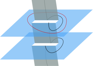
Figure 1: On the Riemann surface used to calculate the Renyi entropy with $N$ replicas (here $N=2$), the black loop must wind $2\pi N$ times before closing onto itself. The red loop surrounds both ends of the cut.

We emphasize that the $U_{q}sl(2)$ spin chain differs from the usual one simply by the boundary terms $h_{i}$. These are not expected to affect the ordinary EE, and the central charge obtained via the density operator $\rho=|0\rangle\langle 0|$ (with $|0\rangle\propto|0_{\rm R}\rangle$, but normalized as in our introduction) will be $c_{\rm eff}=1$.

Entanglement in non-unitary minimal models.

We now discuss the restricted solid-on-solid (RSOS) lattice models, which provide the nicest regularization of non-unitary CFTs. In these models, the variables are “heights” on an $A_{m}$ Dynkin diagram, with Boltzmann weights that provide yet another representation of the TL algebra (8), with parameter $n=2\cos\tfrac{\pi p}{m+1}$ and $p=1,\ldots,m$. The case $p=1$ is Hermitian, while $p\neq 1$ leads to negative weights, and hence a non-unitary CFT. One has $c=1-6{p^{2}\over(m+1)(m+1-p)}$, and, for $p\neq 1$, the effective central charge—determined by the state of lowest conformal weight ISZ through $c_{\rm eff}=c-24h_{\rm min}$—is $c_{\rm eff}=1-{6\over(m+1)(m+1-p)}$ . The case $(m,p)=(4,3)$ gives the Yang-Lee singularity universality class discussed in the introduction.

Defining the EE for RSOS models is not obvious, since their Hilbert space (we use this term even in the non-unitary case) is not a tensor product like for spin chains. Most recent numerical and analytical work however neglected this fact, and EE was defined using a straightforward partial trace, summing over all heights in $B$ compatible with those in $A$. In this case, it was argued and checked numerically that $S_{A}=\tfrac{c}{3}\ln L$ in the unitary case, and $S_{A}=\tfrac{c_{\rm eff}}{3}\ln L$ in the non-unitary case. Note that $c$ matches that of the loop model based on the same TL algebra, with $x+1\equiv{m+1\over p}$. For details on the QG EE in the RSOS case, see the SM.

The RSOS partition functions can be expressed in terms of loop model ones, $Z_{\ell}$. In the plane, the equivalence Pasquier replaces equal-height clusters by their surrounding loops, which get the usual weight $n$ through an appropriate choice of weights on $A_{m}$. With periodic boundary conditions, the correspondence is more intricate due to non-contractible clusters/loops. On the torus DFSZ1 , $Z_{\ell}$ is defined by giving each loop (contractible or not) weight $n$, whereas for the RSOS model contractible loops still have weight $n$, but one sums over sectors where each non-contractible loop gets the weights $n_{k}=2\cos\tfrac{\pi k}{m+1}$ for any $k=1,\ldots,m$. The same sum occurs (see SM for details) when computing $Z^{(N)}$ of the Riemann surface with $N$ replicas: non-contractible loops are here those winding one end of the cut. Note also that $|0_{\rm L}\rangle=|0_{\rm R}\rangle$ for RSOS models, so the imaginary-time definition of $\rho$ in unambiguous Doyon1 ; Doyon2 .

Crucially, the sum over $k$ is dominated (in the scaling limit) by the sector with the largest $n_{k}$, that is $k=1$ and $n_{1}=2\cos\tfrac{\pi}{m+1}$. In the non-unitary case ($p>1$), $n_{1}\neq n$, and the EE is found by extending the above computation. We have still $e_{0}=\tfrac{p}{m+1}$, but now $e=\tfrac{1}{N(m+1)}=\tfrac{e_{0}}{pN}$. To normalize at $N=1$, one must divide by $Z^{(1)}$ to the power $N$, with the same charges:

$$Z^{(N)}/\big{(}Z^{(1)}\big{)}^{N}\propto L^{-\frac{1}{6}\left(N-\frac{1}{N}\right)\big{(}1-\frac{6e_{0}^{2}}{p^{2}g}\big{)}}\,,$$ (10)

whence the Rényi entropy $S_{A}^{(N)}=\tfrac{N+1}{6N}c_{\rm eff}\ln L$. Hence our construction establishes the claim of Doyon1 ; Doyon2 .

EE in the $sl(2|1)$ SUSY chain.

Percolation and other problems with SUSY (see the introduction) have $Z=1$, hence $c=0$, and the EE scales trivially. Having a non-trivial quantity that distinguishes the many $c=0$ universality classes would be very useful. We now show that, by carefully distinguishing left and right eigenstates, and using traces instead of supertraces, one can modify the definition of EE to build such a quantity.

We illustrate this by the $sl(2|1)$ alternating chain ReadSaleur01 which describes percolation hulls. This chain represents the TL algebra (8) with $n=1$, and involves the fundamental ($V$) and its conjugate ($\bar{V}$) on alternating sites, with $\dim V=3$. The 2-site Hamiltonian, $H=-e_{1}$, restricted to the subspace $\{|{1\bar{1}}\rangle,|{2\bar{2}}\rangle,|{3\bar{3}}\rangle\}$ (where $1,2$ are bosonic and $3$ is fermionic), reads

$$e_{1}=|0_{\rm R}\rangle\langle 0_{\rm L}|=\left(|{1\bar{1}}\rangle+|{2\bar{2}}\rangle+|{3\bar{3}}\rangle\right)\left(\langle{1\bar{1}}|+\langle{2\bar{2}}|+\langle{3\bar{3}}|\right)$$

The eigenvectors are $|0_{\rm R}\rangle=|{1\bar{1}}\rangle+|{2\bar{2}}\rangle+|{3\bar{3}}\rangle$ and $\langle 0_{\rm L}|=\langle{1\bar{1}}|+\langle{2\bar{2}}|-\langle{3\bar{3}}|$; note that conjugation is supergroup invariant (i.e., $\langle\bar{3}|{\bar{3}}\rangle=-1$). Hence, despite the misleading expression, $H$ is not unitary. The density operator is $\tilde{\rho}=e_{1}$ and satisfies $\operatorname{STr}\tilde{\rho}\equiv\operatorname{Tr}(-1)^{F}\tilde{\rho}=1$. The reduced density operator $\tilde{\rho}_{A}=\operatorname{STr}_{B}\tilde{\rho}=|{1}\rangle\langle{1}|+|{2}\rangle\langle{2}|+|{3}\rangle\langle{3}|$. If we define the Rényi EE also with the supertrace, we get $\operatorname{STr}\tilde{\rho}_{A}^{N}=1$ for all $N$. It is more interesting (and natural) to take instead the normal trace of $\tilde{\rho}$; this requires a renormalization factor to ensure $\operatorname{Tr}\tilde{\rho}_{A}=1$. We obtain then $\tilde{\rho}_{A}^{N}=\frac{1}{3^{N}}\left(|{1}\rangle\langle{1}|+|{2}\rangle\langle{2}|+|{3}\rangle\langle{3}|\right)$ and thus $\tilde{S}_{A}^{(N)}=\ln 3$. This equals the QG Rényi EE with $n=3$.

This calculation carries over to arbitrary size. One finds that $\tilde{S}_{A}=\tilde{S}_{A,\ell}$ with weight $n=1$, provided non-contractible loops winding around one cut end in the replica calculation get the modified weight $\tilde{n}=3$ instead of $n$. We can then use the CG framework developed in the context of the non-unitary minimal models to calculate the scaling behavior. We use (10), with $g=\tfrac{2}{3}$ for percolation ($n=1$), and $\tilde{n}=2\cos\pi e_{0}$. It follows that $e_{0}$ is purely imaginary, and that $\tilde{S}^{(N)}\thicksim\tfrac{N+1}{6N}c_{\rm eff}\log L$ with $c_{\rm eff}=1+\frac{9}{\pi^{2}}\big{(}\log\frac{3+\sqrt{5}}{2}\big{)}^{2}\thicksim 1.84464\ldots$.

Numerical checks.

All these results were checked numerically. As an illustration, we discuss only the case $q={\rm e}^{2i\pi/5}$, for which the RSOS and loop models have $c=-3/5$, while $c_{\rm eff}=3/5$ for the RSOS model. In the corresponding $U_{q}sl(2)$ chain, we measured the (ordinary) EE as in (3), the QG Rényi EE $\tilde{S}^{(2)}$ as in (7), and the QG Rényi EE for the modified loop model where non-contractible loops have fugacity $n_{1}=2\cos{\pi\over 5}$ (instead of $n=2\cos\frac{2\pi}{5}$). This, recall, should coincide asymptotically with the Rényi EE for the RSOS model. Results (see figure 2) fully agree with our predictions.

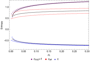
Figure 2: Numerical EE for the non-unitary case $(p,m)=(2,4)$ ($n=2\cos\frac{2\pi}{5}$), versus the length of the cut $L$, for a chain with $M=400$ sites and open boundary conditions. Purple dots show the usual EE with the unmodified trace. Averaging over the parity oscillations (solid curve) reveals the scaling with $c_{\rm XXZ}=1$. Red squares show the $N=2$ Rényi entropy, with the modified trace giving weight $n_{1}=2\cos\pi/5$ to non-contractible loops; this scales with $c_{\rm eff}=3/5$. Blue triangles again show $\tilde{S}^{(2)}$, but with $n_{1}=n$; the scaling then involves the true central charge $c=-3/5$.

Conclusion.

While we have mostly discussed the critical case, we stress that the QG EE can be defined also away from criticality. An interesting example is the $sl(2|1)$ alternating chain, for which staggering makes the theory massive (this corresponds to shifting the topological angle away from $\Theta=\pi$ in the sigma-model representation). Properties of the QG Rényi EE along this (and other) RG flows will be reported elsewhere.

To summarize, we believe that our analysis completes our understanding of EE in 1D by providing a natural extension to non-unitary models in their critical or near-critical regimes. There are clearly many situations (such as phenomenological “Hamiltonians” for open systems) where things will be very different, but we hope our work will provide the first step in the right direction. Our approach also provides a long awaited “Coulomb gas” handle on the correspondence between lattice models and quantum information quantities. In the SM we apply this to show that, in the case of non-compact theories, the well-known ${c\over 3}\ln L$ term will be corrected by $\ln\ln L$ terms (with, most likely, a non-universal amplitude), in agreement with recent independent work BenjaminOlalla .

Acknowledgments: The work of HS and JLJ was supported by the ERC Advanced Grant NuQFT. The work of HS was also supported by the US Department of Energy (grant number DE-FG03-01ER45908). We thank B. Doyon and O. Castro-Alvaredo for inspiring discussions and comments.

I Supplementary Material

In these notes we provide additional details for some results of the main text. We first provide additional motivation for our definition of the entanglement entropy (EE) from the perspective of the $U_{q}sl(2)$ quantum group (QG) symmetry, and we prove that $\tilde{S}_{A}=\tilde{S}_{B}$. Next, we give more examples of the computation of the QG EE for larger larger systems in various representations. We elaborate on the construction in the RSOS case, detailing in particular the mapping between the RSOS and loop model representations. Finally we discuss the emergence of a $\ln(\ln L)$ term in the non-compact case.

I.1 $U_{q}sl(2)$ symmetry for the reduced density operator

Our definition of the EE relies on using a modified trace, known as a Jones trace, in which a factor of the type $q^{-2S\sigma^{z}_{B}}$ is inserted under the usual trace symbol. To ensure that the resulting reduced density operator $\rho_{A}$ makes sense in the QG formalism, we must ensure that it commutes with the generators of $U_{q}sl(2)$.

We therefore consider the XXZ spin-$1/2$ chain, with boundary terms as described in the main text. The Hamiltonian commutes with the following generators:

$$S^{z} = \sum_{i}\sigma_{i}^{z}$$ (11)

$$S^{+} = \frac{1}{2}\sum_{i}q^{\sigma_{1}^{z}}\!\otimes\!...\!\otimes\!q^{\sigma_{i-1}^{z}}\!\otimes\!\sigma_{i}^{+}\!\otimes\!q^{-\sigma_{i+1}^{z}}\!\otimes\!...\!\otimes\!q^{-\sigma_{M}^{z}}$$ (12)

$$S^{-} = \frac{1}{2}\sum_{i}q^{\sigma_{1}^{z}}\!\otimes\!...\!\otimes\!q^{\sigma_{i-1}^{z}}\!\otimes\!\sigma_{i}^{-}\!\otimes\!q^{-\sigma_{i+1}^{z}}\!\otimes\!...\!\otimes\!q^{-\sigma_{M}^{z}}$$ (13)

Since the generators commute with the Hamiltonian, they share the same right and left eigenvectors. As a consequence they commute with the density operator $\rho$

$$[S^{\alpha},\rho]=0,\qquad\rho=|{0_{\rm R}}\rangle\langle{0_{\rm L}}|\,.$$ (14)

We split the spin chain in two parts $A$, $B$ and define the reduced density operator $\rho_{A}$ using a Jones trace over the part $B$. We consider the case where $A$ is in the middle of the chain between $B_{\rm L}$ and $B_{\rm R}$, so that $B=B_{\rm L}\cup B_{\rm R}$ and $\mathcal{H}=\mathcal{H}_{B_{\rm L}}\otimes\mathcal{H}_{A}\otimes\mathcal{H}_{B_{\rm R}}$. Thus

$$\rho_{A}=\operatorname{Tr}_{B}\ q^{2S^{z}_{B_{\rm L}}-2S^{z}_{B_{\rm R}}}\rho\,,\quad\mbox{with }S^{z}_{B}=\sum_{i\in B}\sigma_{i}^{z}\,.$$ (15)

Let us check that the generators of $U_{q}(sl_{2})$ on the subsystem $A$ commute with the reduced density operator $\rho_{A}$. We have the following relations:

$$S^{z}\! = \!S^{z}_{B_{\rm L}}\otimes\mathds{1}+\mathds{1}\otimes S^{z}_{A}\otimes\mathds{1}+\mathds{1}\otimes S^{z}_{B_{\rm R}}\,,$$ (16)

$$S^{\pm}\! = \!S^{\pm}_{B_{\rm L}}q^{-S^{z}_{A}-S^{z}_{B_{\rm R}}}\!+\!q^{S^{z}_{B_{\rm L}}}S^{\pm}_{A}q^{-S^{z}_{B_{\rm R}}}\!+\!q^{S^{z}_{B_{\rm L}}+S^{z}_{A}}S^{\pm}_{B_{\rm R}}\,.$$

Consider first $S^{z}_{A}$:

$$S^{z}_{A}\ \rho_{A} = \operatorname{Tr}_{B}\left(S^{z}_{A}q^{2S^{z}_{B_{\rm L}}-2S^{z}_{B_{\rm R}}}\rho\right)$$

$$= \operatorname{Tr}_{B}\left((S^{z}-S^{z}_{B_{\rm L}}-S^{z}_{B_{\rm R}})q^{2S^{z}_{B_{\rm L}}-2S^{z}_{B_{\rm R}}}\rho\right)\,.$$

Obviously $S^{z}_{B_{\rm L}}$, $S^{z}_{B_{\rm R}}$, $S^{z}_{A}$ and $S^{z}$ commute. Since $S^{z}$ also commutes with $\rho$:

$$S^{z}_{A}\ \rho_{A} = \operatorname{Tr}_{B}\left(q^{2S^{z}_{B_{\rm L}}-2S^{z}_{B_{\rm R}}}\rho S^{z}\right)-\operatorname{Tr}_{B}\left(q^{2S^{z}_{B_{\rm L}}-2S^{z}_{B_{\rm R}}}\rho S^{z}_{B_{\rm L}}\right)$$

$$- \operatorname{Tr}_{B}\left(q^{2S^{z}_{B_{\rm L}}-2S^{z}_{B_{\rm L}}}\rho S^{z}_{B_{\rm L}}\right)\,.$$

For the two last terms we performed a cyclic permutation under the trace. We can now sum all terms and this proves $\left[S^{z}_{A},\rho_{A}\right]=0$. Next we do the same for $S^{+}_{A}$:

$$S^{+}_{A}\ \rho_{A} = \operatorname{Tr}_{B}\left(S^{+}_{A}\rho\ q^{2S^{z}_{B_{\rm L}}-2S^{z}_{B_{\rm R}}}\right)$$ (18)

$$= \operatorname{Tr}_{B}\Big{(}(q^{-S^{z}_{B_{\rm L}}+S^{z}_{B_{\rm R}}}S^{+}-q^{-S^{z}_{A}-S^{z}_{B_{\rm L}}}S^{+}_{B_{\rm L}}$$

$$-q^{S^{z}_{A}+S^{z}_{B_{\rm R}}}S^{+}_{B_{\rm R}})\rho q^{2S^{z}_{B_{\rm L}}-2S^{z}_{B_{\rm R}}}\Big{)}$$

$$\equiv (1)-(2)-(3)\,.$$

The first term $(1)$ of the right-hand side reads

$$(1) = \operatorname{Tr}_{B}\Big{(}q^{-S^{z}_{B_{\rm L}}+S^{z}_{B_{\rm R}}}S^{+}\rho q^{2S^{z}_{B_{\rm L}}-2S^{z}_{B_{\rm R}}}\Big{)}$$

$$= \operatorname{Tr}_{B}\Big{(}q^{2S^{z}_{B_{\rm L}}-2S^{z}_{B_{\rm R}}}\rho S^{+}q^{-S^{z}_{B_{\rm L}}+S^{z}_{B_{\rm R}}}\Big{)}$$

thanks to the cyclic permutation under the trace and the commutation of $\rho$ and $S^{+}$. We then deal with the second term $(2)$ involving $S^{+}_{B_{\rm L}}$:

$$(2) = \operatorname{Tr}_{B}\Big{(}q^{-S^{z}_{A}-S^{z}_{B_{\rm L}}}S^{+}_{B_{\rm L}}\rho q^{2S^{z}_{B_{\rm L}}-2S^{z}_{B_{\rm R}}}\Big{)}$$

$$= \operatorname{Tr}_{B}\Big{(}S^{+}_{B_{\rm L}}q^{-S^{z}_{A}}\rho q^{S^{z}_{B_{\rm L}}-2S^{z}_{B_{\rm R}}}\Big{)}$$

$$= \operatorname{Tr}_{B}\Big{(}q^{-S^{z}+S^{z}_{B_{\rm R}}+S^{z}_{B_{\rm L}}}\rho q^{S^{z}_{B_{\rm L}}-2S^{z}_{B_{\rm R}}}S^{+}_{B_{\rm L}}\Big{)}$$

$$= \operatorname{Tr}_{B}\Big{(}q^{-S^{z}_{B_{\rm R}}+S^{z}_{B_{\rm L}}}\rho q^{-S^{z}+S^{z}_{B_{\rm L}}}S^{+}_{B_{\rm L}}\Big{)}$$

$$= \operatorname{Tr}_{B}\Big{(}q^{-2S^{z}_{B_{\rm R}}+2S^{z}_{B_{\rm L}}}\rho S^{+}_{B_{\rm L}}q^{-S^{z}_{A}-S^{z}_{B_{\rm L}}}\Big{)}\,,$$

thanks to cyclic permutations of the operators over the subsystem $B$, the commutation of $S^{z}$ with $\rho$ and the commutation of $S^{z}_{B_{\rm L}}$ with $S^{z}_{A}$ and $S^{z}_{B_{\rm R}}$. Similarly for the term $(3)$ involving $S^{+}_{B_{\rm R}}$:

$$(3) = \text{Tr}_{B}\Big{(}q^{S^{z}_{A}+S^{z}_{B_{\rm R}}}S^{+}_{B_{\rm R}}\rho q^{2S^{z}_{B_{\rm L}}-2S^{z}_{B_{\rm R}}}\Big{)}$$

$$= \text{Tr}_{B}\Big{(}q^{-2S^{z}_{B_{\rm R}}+2S^{z}_{B_{\rm L}}}\rho S^{+}_{B_{\rm R}}q^{S^{z}_{A}+S^{z}_{B_{\rm R}}}\Big{)}\,.$$

By regrouping the terms we find the desired property $S^{+}_{A}\rho_{A}=\rho_{A}S^{+}_{A}$. A very similar computation can be done for $S^{-}_{A}$.

I.2 Proof of $\tilde{S}_{A}=\tilde{S}_{B}$

A meaningful EE must satisfy, at the very least, the symmetry property $S_{A}=S_{B}$, meaning that subsystem $A$ is as entangled with $B$, as $B$ with $A$. We now show that this is the case for our QG EE.

Let us consider the case $q\in\mathbb{R}$. The proof is then simple and can be extended by analytic continuation to complex $q$. In this case the Hamiltonian is symmetric, and $|{0}\rangle\equiv|{0_{\rm R}}\rangle=|{0_{\rm L}}\rangle$. We again divide our system in two pieces $A$ and $B$ with a cut in the middle (for more complicated cuts the argument is similar) and write the state in the following way:

$$|{0}\rangle=\sum_{i,j}\psi_{i,j}|{i}\rangle_{A}|{j}\rangle_{B}\,.$$ (19)

The bases $|{i}\rangle_{A}$ and $|{j}\rangle_{B}$ can be chosen such that they have a well-defined magnetization. As a consequence, since the groundstate $|0\rangle$ is in the zero-magnetization sector, we can define those bases such that the matrix $\psi_{i,j}$ is block-diagonal and where each block corresponds to a sector of $A$ and $B$ with a well-defined magnetization. When we perform a singular value decomposition (SVD) we end up with

$$|{0}\rangle=\sum_{\alpha}s_{\alpha}|{\alpha}\rangle_{A}|{\alpha}\rangle_{B}\,,$$ (20)

where $|{\alpha}\rangle_{A}$ and $|{\alpha}\rangle_{B}$ are eigenvectors of $S_{A}$ and $S_{B}$; they form orthonormal bases of $A$ and $B$. The density matrix $\rho$ is

$$\rho=\sum_{\alpha,\alpha^{\prime}}s_{\alpha}s_{\alpha^{\prime}}|{\alpha}\rangle_{A}|{\alpha}\rangle_{B}\langle{\alpha^{\prime}}|_{A}\langle{\alpha^{\prime}}|_{B}\,.$$ (21)

The reduced density matrices $\rho_{A}$ and $\rho_{B}$ read

$$\rho_{A} = \operatorname{Tr}_{B}q^{-2S_{B}}\rho=\sum_{\alpha}s_{\alpha}^{2}q^{-2S^{\alpha}_{B}}|{\alpha}\rangle_{A}\langle{\alpha}|_{A}\,,$$

$$\rho_{B} = \operatorname{Tr}_{A}q^{-2S_{A}}\rho=\sum_{\alpha}s_{\alpha}^{2}q^{2S^{\alpha}_{A}}|{\alpha}\rangle_{B}\langle{\alpha}|_{B}\,.$$

Since the ground state is in the $S=0$ sector $q^{2S^{\alpha}_{A}}=q^{-2S^{\alpha}_{B}}$ and thus the two reduced density operators have the same spectra and define the same entropy. This proves the statement $\tilde{S}_{A}=\tilde{S}_{B}$ in the case of a cut in the middle of the system.

I.3 More examples

To keep the discussion in the main text as simple as possible, we have presented all explicit computations for a chain with just $M=2$ sites. This is of course no limitation to applying our general definitions, and accordingly we give here a few examples for higher values of $M$.

I.3.1 Loop representation

We consider the case of $M=4$ sites. The basis of link states is :

$$|{1}\rangle=\quad\leavevmode\hbox to26.41pt{\vbox to5.07pt{\text{[drawing]}}}\quad,\qquad|{2}\rangle=\quad\leavevmode\hbox to26.41pt{\vbox to9.34pt{\text{[drawing]}}}\quad$$ (22)

The hamiltonian $H=-e_{1}-e_{2}-e_{3}$ has the following ground state $|{0}\rangle=\frac{1}{{\cal N}}(\alpha|{1}\rangle+|{2}\rangle)$, where ${\cal N}^{2}=n^{2}\alpha^{2}+2n\alpha+n^{2}$ and $\alpha=(n+\sqrt{n^{2}+8})/2$. The density matrix $\rho$ is

$$\rho=\frac{1}{{\cal N}^{2}}\Big{(}\alpha^{2}\!\!\!\!\raisebox{6.00006pt}{\quad \leavevmode\hbox to26.41pt{\vbox to13.6pt{\text{[drawing]}}}\quad}\!\!\!\!+\alpha\!\!\!\!\raisebox{6.00006pt}{\quad \leavevmode\hbox to26.41pt{\vbox to13.6pt{\text{[drawing]}}}\quad}\!\!\!\!+\alpha\!\!\!\!\raisebox{6.00006pt}{\quad \leavevmode\hbox to26.41pt{\vbox to13.6pt{\text{[drawing]}}}\quad}\!\!\!\!+\!\!\!\!\raisebox{6.00006pt}{\quad \leavevmode\hbox to26.41pt{\vbox to13.6pt{\text{[drawing]}}}\quad}\!\!\!\!\Big{)}\,.$$

Consider first a bipartition in which $A$ is the first site, and $B$ the remainder. Take the partial Markov trace over the three last sites, we find the reduced density operator

$$\rho_{A}=\frac{1}{{\cal N}^{2}}(\alpha^{2}n+2\alpha+n)\!\!\!\!\quad\leavevmode\hbox to0.8pt{\vbox to15.03pt{\text{[drawing]}}}\quad\!\!\!\!=\frac{1}{n}\!\!\!\!\quad\leavevmode\hbox to0.8pt{\vbox to15.03pt{\text{[drawing]}}}\quad\,.$$ (23)

This leads to $\tilde{S}_{A}=\log n$, the same result as found in the main text for the EE of the first spin with $M=2$.

Next we take $A$ as the first two sites, to compute the entanglement at the middle of the system. We trace the density operator over the two last sites:

$$\rho_{A} = \frac{1}{{\cal N}^{2}}\Big{(}\ \leavevmode\hbox to9.34pt{\vbox to13.6pt{\text{[drawing]}}}+(\alpha^{2}n+2\alpha)\leavevmode\hbox to9.34pt{\vbox to13.6pt{\text{[drawing]}}}\Big{)}$$ (24)

$$= \frac{1}{{\cal N}^{2}}\big{(}\mathbb{I}+(\alpha^{2}n+2\alpha)e_{1}\big{)}\,.$$

We now need to take the logarithm of $\rho_{A}$. We notice the identity $\exp(a\,e_{1})=1+\frac{1}{n}(\exp(an)-1)e_{1}$, where $e_{1}=\leavevmode\hbox to7.91pt{\vbox to9.34pt{\text{[drawing]}}}$. It is then easy to find that

$$\log\rho_{A}=-\log{\cal N}^{2}\,\mathbb{I}+\frac{2}{n}\log(1+\alpha n)e_{1}\,.$$ (25)

We can now compute $\rho_{A}\log\rho_{A}$ as

$$- \frac{\log{\cal N}^{2}}{{\cal N}^{2}}\ \leavevmode\hbox to9.34pt{\vbox to13.6pt{\text{[drawing]}}}+\Big{(}\frac{-\log{{\cal N}^{2}}}{{\cal N}^{2}}(\alpha^{2}n+2\alpha)+\frac{2}{n{\cal N}^{2}}\log(1+\alpha n)$$ (26)

$$+ \frac{2}{{\cal N}^{2}}(\alpha^{2}n+2\alpha)\log(1+\alpha n)\Big{)}\leavevmode\hbox to9.34pt{\vbox to13.6pt{\text{[drawing]}}}\,.$$

Tracing over $A$ we finally obtain

$$\tilde{S}_{A} = -\operatorname{Tr}\rho_{A}\log\rho_{A}=\frac{n^{2}\log{\cal N}^{2}}{{\cal N}^{2}}-n\Big{(}\frac{-\log{{\cal N}^{2}}}{{\cal N}^{2}}(\alpha^{2}n+2\alpha)$$ (27)

$$+ \frac{2}{n{\cal N}^{2}}\log(1+\alpha n)+\frac{2}{{\cal N}^{2}}(\alpha^{2}n+2\alpha)\log(1+\alpha n)\Big{)}$$

$$= -\frac{(1+\alpha n)^{2}}{{\cal N}^{2}}\log(1+\alpha n)^{2}+\log{\cal N}^{2}\,.$$

We have verified that this expression coincides with the result obtained by using the modified trace in the vertex model. It also agrees with computations in the Potts spin representation for $Q=n^{2}$ integer (see below).

For larger $M$ it is hard to compute this final partial trace directly, since the form of $\log\rho_{A}$ will be substantially more complicated than (25). A much more convenient option is to recall that gluing corresponding sites on top and bottom of any word in the TL algebra means technically to take the so-called Markov trace $\operatorname{MTr}$. This in turn can be resolved as follows

$$\operatorname{MTr}\ =\sum_{j}[2j+1]_{q}\operatorname{Tr}_{{\cal V}_{j}}\,,$$ (28)

where $\operatorname{Tr}_{{\cal V}_{j}}$ is the usual matrix trace over the (standard) module ${\cal V}_{j}$ with $2j$ defect lines, and $[k]_{q}=\tfrac{q^{k}-q^{-k}}{q-q^{-1}}$ are $q$-deformed numbers such that the loop weight $n=[2]_{q}=q+q^{-1}$.

In the simple $M=4$ case considered above, $A$ has just two sites so that ${\cal V}_{0}$ and ${\cal V}_{1}$ are both one-dimensional with bases $\{\leavevmode\hbox to7.91pt{\vbox to4.36pt{\text{[drawing]}}}\}$ and $\{\leavevmode\hbox to7.91pt{\vbox to7.91pt{\text{[drawing]}}}\}$ respectively. Thus we have the matrices

$$\left.\rho_{A}\right|_{{\cal V}_{0}}=\left[\frac{1}{{\cal N}^{2}}(1+n\ (\alpha^{2}n+2\alpha))\right]\,,\quad\left.\rho_{A}\right|_{{\cal V}_{2}}=\left[\frac{1}{{\cal N}^{2}}\right]$$

and

$$\operatorname{MTr}\rho_{A}\log\rho_{A} = \operatorname{Tr}_{{\cal V}_{0}}\rho_{A}\log\rho_{A}$$ (29)

$$+ (n^{2}-1)\operatorname{Tr}_{{\cal V}_{2}}\rho_{A}\log\rho_{A}\,.$$

We find in the end

$$\operatorname{MTr}\rho_{A}\log\rho_{A} = \frac{(1+\alpha n)^{2}}{N^{2}}\log\frac{(1+\alpha n)^{2}}{{\cal N}^{2}}$$ (30)

$$+ (n^{2}-1)\frac{1}{{\cal N}^{2}}\log{\frac{1}{{\cal N}^{2}}}\,,$$

which is the same as (27) after simplification.

We have made similar computations for $M=6$ sites, for all choises of the bipartition $A\cup B$, finding again perfect agreement between the results from the loop model (with the Markov trace) and the vertex model (with the modified trace).

I.3.2 Spin representation

The same computation can be conducted in the $Q$-state Potts spin representation for $Q$ integer. There are ${\cal L}=M/2$ spins labelled $S_{j}$ (with $j=1,2,\ldots,{\cal L}$) enjoying free boundary conditions. The interactions $e_{i}$ take different expressions depending on the parity of $i$. We have $e_{2j-1}=Q^{-1/2}D_{j}$, where $D_{j}$ detaches the $j$’th spin from the rest (the new spin freely takes any of the $Q$ values); while $e_{2j}=Q^{1/2}J_{j}$, where $J_{j}=\delta(S_{j},S_{j+1})$ joins two neighbouring spins (forcing them to take the same value).

In the above $M=4$ example, the Hamiltonian is

$$H=-Q^{-1/2}(D_{1}+D_{2})-Q^{1/2}J_{1}\,,$$ (31)

and for $Q=2$ the interactions read explicitly, in the basis $\left\{|++\rangle,|+-\rangle,|-+\rangle,|--\rangle\right\}$,

$$D_{1}=\left(\begin{smallmatrix}1&0&1&0\\ 0&1&0&1\\ 1&0&1&0\\ 0&1&0&1\\ \end{smallmatrix}\right)\,,\quad D_{2}=\left(\begin{smallmatrix}1&1&0&0\\ 1&1&0&0\\ 0&0&1&1\\ 0&0&1&1\\ \end{smallmatrix}\right)\,,\quad J_{1}=\left(\begin{smallmatrix}1&0&0&0\\ 0&0&0&0\\ 0&0&0&0\\ 0&0&0&1\\ \end{smallmatrix}\right)\,.$$

The normalised ground state is

$$|0\rangle=k^{-}\left(|++\rangle+|--\rangle\right)+k^{+}\left(|+-\rangle+|-+\rangle\right)\,,$$ (32)

with $k^{\pm}=(5\pm\sqrt{5})^{-1/2}$. Tracing over the subsystem $B$ (the right spin $S_{2}$) we find the reduced density matrix

$$\rho_{A}=\left(\begin{array}[]{cc}(k^{+})^{2}+(k^{-})^{2}&2k^{+}k^{-}\\ 2k^{+}k^{-}&(k^{+})^{2}+(k^{-})^{2}\end{array}\right)=\left(\begin{array}[]{cc}\frac{1}{2}&\frac{1}{\sqrt{5}}\\ \frac{1}{\sqrt{5}}&\frac{1}{2}\end{array}\right)\,,$$

where of course $\operatorname{Tr}\rho_{A}=1$. The eigenvalues are $\lambda^{\pm}=\frac{1}{2}\pm\frac{1}{\sqrt{5}}$. Thus

$$\tilde{S}_{A} = -\left(\lambda^{+}\log\lambda^{+}+\lambda^{-}\log\lambda^{-}\right)$$ (33)

$$= \log\left(2\sqrt{5}\right)+\frac{1}{\sqrt{5}}\log\left(9-4\sqrt{5}\right)\,,$$

which is easily seen to agree with (27) for $Q=2$.

Let us note that the eigenenergies of (31) are $-(3\pm\sqrt{5})/\sqrt{2},-2\sqrt{2},-\sqrt{2}$. The first two (and in particular the ground state energy) are also found in the loop model, but the latter two are not. As we have seen, this does not prevent us from finding the same $S$, which is a property of $|0\rangle$. On the other hand, one can check that $\rho_{A}$ has the same spectrum in the two representations. These conclusions extend to $Q=3$: we find the same $\tilde{S}_{A}$, and the eigenvalues of $\rho_{A}$ are the same (up to multiplicities, and after the elimination of non-relevant zero eigenvalues).

I.3.3 RSOS representation

In the RSOS construction a height $h_{i}=1,2,\ldots,m$ is defined at each site $i=0,1,\ldots,M$, subject to the constraint $|h_{i}-h_{i-1}|=1$ for each $1<i\leq M$. We note that while the loop model is defined on $M$ strands, there are now $M+1$ RSOS heights.

Free boundary conditions for the first and last spins in the equivalent Potts model (i.e., no defect lines in the loop model) correspond BauerSaleur89 to fixing $h_{0}=h_{M}=1$. More generally, having $2j$ defect lines in the loop model would correspond to $h_{0}=1$ and $h_{M}=1+2j$.

To explain the details we move to a slightly larger example, namely $M=6$ and $m=5$ (i.e., $Q=3$), in order to see all non-trivial features of the computation at work. Consider the following labelling of the RSOS basis states:

$$|1\rangle = \{1,2,3,2,3,2,1\}\,,\quad|2\rangle=\{1,2,3,2,1,2,1\}\,,$$

$$|3\rangle = \{1,2,3,4,3,2,1\}\,,\quad|4\rangle=\{1,2,1,2,3,2,1\}\,,$$

$$|5\rangle = \{1,2,1,2,1,2,1\}\,.$$ (34)

It is straightforward to find the normalised ground state $|0\rangle$ in this basis and check that its eigenenergy coincides with that of the other representations. We denote $\rho=|0\rangle\langle 0|$ as usual.

Consider first the bipartion “4+2”, where $A$ contains the first four sites and $B$ the last two. The junction of the two intervals is at $i^{*}=4$, and we write $h_{i^{*}}=1+2j$ for the corresponding intermediate height which belongs to both $A$ and $B$. The sector $j=0$ has the basis $\{|2\rangle,|5\rangle\}$, while $j=1$ has the basis $\{|1\rangle,|3\rangle,|4\rangle\}$. In each sector, the reduced density matrix $\left.\rho_{A}\right|_{{\cal V}_{j}}$ is formed by tracing over the heights belonging to $B$. However, in both cases the choice of boundary conditions ($h_{M}=1$), the sector label $j$ and the RSOS constraint fully fix the $B$-heights, so the trace is trivial:

$$\left.\rho_{A}\right|_{{\cal V}_{0}} = \left(\begin{array}[]{cc}\langle 2|\rho|2\rangle&\langle 2|\rho|5\rangle\\ \langle 5|\rho|2\rangle&\langle 5|\rho|5\rangle\end{array}\right)\,,$$ (37)

$$\left.\rho_{A}\right|_{{\cal V}_{1}} = \left(\begin{array}[]{ccc}\langle 1|\rho|1\rangle&\langle 1|\rho|3\rangle&\langle 1|\rho|4\rangle\\ \langle 3|\rho|1\rangle&\langle 3|\rho|3\rangle&\langle 3|\rho|4\rangle\\ \langle 4|\rho|1\rangle&\langle 4|\rho|3\rangle&\langle 4|\rho|4\rangle\\ \end{array}\right)\,.$$ (41)

Each $\left.\rho_{A}\right|_{{\cal V}_{j}}$ has precisely one non-zero eigenvalue, $\Lambda_{j}$. Applying the normalisation

$$\lambda_{j}=\Lambda_{j}/[1+2j]_{q}$$ (42)

we find that they agree with the eigenvalues of $\rho_{A}$ restrained to the standard module ${\cal V}_{j}$ with $2j$ defect lines in the corresponding loop model computation. Therefore $S$ can be computed by the decomposition (28) of the Markov trace, which writes explicitly as (29) in this simple case.

To see a non-trivial trace over the $B$-system, we consider the same example but with the “3+3” bipartition (i.e., $i^{*}=3$). The sector $j=\frac{1}{2}$ has the basis (for the $A$-heights) $\{|1,2,1,2\rangle,|1,2,3,2\rangle\}$. The first basis element corresponds to states $|5\rangle$ and $|4\rangle$ for the full system, while the second basis elements corresponds to $|1\rangle$ and $|2\rangle$. Therefore, to form $\rho_{A}\left(\frac{1}{2}\right)$ we must sum over those possibilities (which corresponds to tracing over the free height $h_{5}=1,3$):

$$\rho_{A}\left(\frac{1}{2}\right)=\left(\begin{array}[]{cc}\langle 5|\rho|5\rangle+\langle 4|\rho|4\rangle&\langle 5|\rho|2\rangle+\langle 4|\rho|1\rangle\\ \langle 2|\rho|5\rangle+\langle 1|\rho|4\rangle&\langle 2|\rho|2\rangle+\langle 1|\rho|1\rangle\\ \end{array}\right)\,.$$ (43)

The remainder of the computation proceeds as outlined above, and the end result again agrees with that of the loop model.

I.4 Extracting the real central charge in the non-unitary case

We describe now the general construction of a modified trace in the RSOS models that will enable us to extract the true central charge from the entanglement, even in the non-unitary case. We thus return to the $A_{m}$ RSOS model with $n=2\cos\frac{\pi p}{m+1}$ and ${\rm gcd}(p,m+1)=1$.

Set $S_{h}=\sin\frac{\pi ph}{m+1}$. The interactions $e_{i}$ satisfying (8) propagate $h_{i}$ into $h^{\prime}_{i}$ and read $e_{i}=\delta_{h_{i-1},h_{i+1}}\sqrt{S_{h_{i}}S_{h^{\prime}_{i}}}/S_{h_{i-1}}$. With the boundary conditions $h_{0}=h_{M}=1$, the ground state $|0\rangle$ then has the same energy as in the other representations—this is also true in the non-unitary cases $p>1$, provided we resolve the square root as $\sqrt{S_{h_{i}}S_{h^{\prime}_{i}}}=S_{h_{i}}$ when $S_{h_{i}}=S_{h^{\prime}_{i}}<0$.

Obtaining the reduced density matrix $\rho_{A}$ for a bipartition $A\cup B$ involves a subtle manipulation of the height $h_{i^{*}}$ situated at the junction between $A$ and $B$. For each fixed $h_{i^{*}}\equiv 1+2j$, define $\rho_{A}(j)$ as the usual trace of $\rho=|0\rangle\langle 0|$ over the $B$-heights ($h_{i}$ with $i>i^{*}$). Thus $\rho_{A}(j)$ is a matrix indexed by the $A$-heights ($h_{i}$ with $i<i^{*}$). The label $j$ is the quantum group spin of the sector $\rho_{A}(h_{j})$ of the reduced density matrix, and corresponds to having $2j$ defect lines in the loop model computation. Now let $\{\Lambda_{k}(j)\}$ denote the set eigenvalues of $\rho_{A}(j)$. We claim that $\lambda_{k}(j)=\Lambda_{k}(j)/[1+2j]_{q}$ yield precisely the corresponding loop model eigenvalues (disregarding any zero eigenvalues), and that the QG entropy $\tilde{S}=-\operatorname{MTr}\rho_{A}\log\rho_{A}$ can be constructed therefrom by computing the Markov trace (28) over $A$ in the same way as for the loop model.

Note that this implies the following relation

$$- \sum_{j,k}[2j+1]_{q}\lambda_{k}(j)\ln\lambda_{k}(j)=$$

$$- \sum_{j,k}\Lambda_{k}(j)\ln\Lambda_{k}(j)+\sum_{j,k}\Lambda_{k}(j)\ln[2j+1]_{q}\,,$$

where on the left we have the QG EE, and the first term on the right is the ‘ordinary’ EE for the (non-unitary) RSOS model. The term on the left scales like $\frac{c}{6}\ln L$, and the first term on the right like $\frac{c_{\rm eff}}{6}\ln L$. This implies that the second term on the right must also be proportional to $\ln L$ in the non-unitary case. While this is not impossible in view of our knowledge of entanglement spectra LefCal , the result clearly deserves a more thorough study.

I.5 The detailed calculation in the RSOS case

We discuss here in more detail the correspondence between the RSOS and loop models for the calculation of the Rényi entropies. For simplicity, we only consider open boundary conditions with the boundary heights $h_{\rm bdy}$ fixed to $1$ and a cut on the edge of the system (Figure 3). Loops surround clusters of constant height. When a loop makes a right (resp. left) turn by bouncing off a piece of a cluster, it gets a weight $\sqrt{S_{a}/S_{b}}$ (resp. $\sqrt{S_{b}/S_{a}}$) where $a$ and $b$ are the heights of the adjacent clusters (cluster of height $b$ on the left, and $a$ on the right). The amplitude $S_{h}$ is defined by $S_{h}=\frac{\sin h\lambda}{\sin\lambda}$, with $\lambda=\frac{p\pi}{m+1}$. After summing over all possible heights, loops pick a weight $n=2\cos\frac{p\pi}{m+1}=\frac{S_{h-1}+S_{h+1}}{S_{h}}$ if they are homotopic to a point.

Figure 3: Surface with $N=2$ replicas. Black edges along the planes represent boundary conditions (height fixed to $h_{\rm bdy}$). The top and bottom are identified. Non-contractible loops always wind $N$ times. Moreover, only the outermost loop (red here) sees the boundary directly.

Let us consider the Rényi entropies for $N>1$. Using the replica picture, we must compute the weigh of loops on the $N$-sheeted surface shown in Figure 3 for $N=2$. The weight of a non-contractible (resp. contractible) loop on this surface is $\left(S_{h^{\prime}}/S_{h}\right)^{N}$ (resp. $S_{h^{\prime}}/S_{h}$), due to the $2\pi N$ winding of non-contractible loops; this must finally be summed over all possible path in the Dynkin diagram. For instance, consider the case of Figure 3, with $N=2$ and two non-contractible loops. The first loop is the boundary between a cluster of height $h_{\rm bdy}=1$ on its left and $2$ on its right. It picks up a factor $S_{2}^{2}/S_{1}^{2}$. The second loop can either surround a cluster of height $1$ or $3$, and therefore gets a factor $(S_{3}^{2}+S_{1}^{2})/S_{2}^{2}$.

In the general case, we consider heights living on the $A_{m}$ Dynkin diagram, and define the following matrix $\left(\Lambda_{N}\right)_{i,j}=\delta_{|i-j|,1}\left(S_{i}/S_{j}\right)^{N}$ for $i,j=1,\ldots,m$. Thus, $\Lambda_{N}$ is the adjacency matrix with the non-contractible loop weights on $N$ replicas. The matrix element $(\Lambda_{N}^{k})_{h_{\rm bdy},h_{k}}$ is the weight of the configuration with $k$ non-contractible loops, where the boundaries are fixed to $h_{\rm bdy}$ and the last loop surrounds a cluster of height $h_{k}$. Since we sum over the height of the last cluster and we fixed $h_{\rm bdy}=1$, the full weight is $\langle{{\bf h}_{\rm free}}|\Lambda_{N}^{k}|{{\bf h}_{\rm bdy}}\rangle$ where $\langle{{\bf h}_{\rm free}}|=\left(1,\ldots,1\right)$ and $|{{\bf h}_{\rm bdy}}\rangle=\left(1,0,\ldots,0\right)^{T}$. The weight of a set of $k$ contractible loops is then $w=\sum_{i=1}^{m}\langle{\bf h}_{\rm free}|\lambda_{i}\rangle\langle\lambda_{i}|{\bf h}_{\rm bdy}\rangle\lambda_{i}^{k}$, where $|{\lambda_{i}}\rangle$ and $\langle{\lambda_{i}}|$ are the right and left eigenvectors of $\Lambda_{N}$ associated to the eigenvalues $\lambda_{i}$, for $i=1,\ldots,m$.

We hence need to sum over sectors where the weight of non-contractible loops is given by the different eigenvalues of $\Lambda_{N}$. We notice that the characteristic polynomial depends only on the products $\left(\Lambda_{N}\right)_{i,j}\left(\Lambda_{N}\right)_{j,i}=1$ (expand by the minors of the first column). The characteristic polynomial is hence unchanged if we replace $\Lambda_{N}$ by the usual adjacency matrix, with elements $\Lambda_{i,j}=\delta_{|i-j|,1}$. The spectra of the adjacency matrices of $A_{m}$ Dynkin diagrams are $\{\lambda_{k}=2\cos\frac{k\pi}{m+1}\}_{k=1,\ldots,m}$. The normalized eigenvectors of $\Lambda_{N}$ are found BauerSaleur89 as

$$|{\lambda_{k}}\rangle_{i} = \sqrt{\frac{2}{m+1}}\left(\frac{\sin\frac{ip\pi}{m+1}}{\sin\frac{p\pi}{m+1}}\right)^{N}\sin\left(\frac{ik\pi}{m+1}\right)\,,$$

$$\langle{\lambda_{k}}|_{i} = \sqrt{\frac{2}{m+1}}\left(\frac{\sin\frac{ip\pi}{m+1}}{\sin\frac{p\pi}{m+1}}\right)^{-N}\sin\left(\frac{ik\pi}{m+1}\right)$$ (45)

for $i=1,2,\ldots,m$. Finally, the RSOS partition function with $N$ replicas and a boundary is a sum of loop partition functions $Z_{N,k}^{\rm loop}$, where non-contractible loops get a weight $\lambda_{k}$, i.e., $Z_{N}^{\rm RSOS}=\sum_{k=1}^{m}\alpha_{k}Z_{N,k}^{\rm loop}$. The prefactor $\alpha_{k}$ can be computed from the eigenvectors of $\Lambda_{N}$:

$$\alpha_{k} = \langle{\bf h}_{\rm free}|\lambda_{k}\rangle\langle\lambda_{k}|{\bf h}_{\rm bdy}\rangle$$

$$= \frac{2}{m+1}\left(\sin\frac{h_{\rm bdy}k\pi}{m+1}\right)^{1-N}\sum_{i=1}^{m}\left(\sin\frac{ip\pi}{m+1}\right)^{N}\sin\frac{ik\pi}{m+1}\,.$$

The dominant contribution comes from non-contractible loop with the largest possible weight, $2\cos{\frac{\pi}{1+m}}$; this is because the corresponding sector is associated with the smallest electric charge. In the limit where the system size goes to infinity we thus have $Z_{N}^{\rm RSOS}\thicksim\alpha_{1}Z_{1}^{\rm loop}$.

We note that the detailed coefficient $\alpha_{k}$ will depend on the boundary condition imposed on the left of the system. For fixed height $h_{\rm bdy}$, we see that the prefactor in (I.5) contributes a term $\ln\big{(}\sin\frac{h_{\rm bdy}k\pi}{m+1}\big{)}$. Recall now the expression (see e.g. Freden ) of the Affleck-Ludwig entropy AffLud —we restrict here to the unitary case $p=1$ for simplicity:

$$g_{1h_{\rm bdy}}=\left[{2\over m(m+1)}\right]^{1/4}\left[2{\sin{\pi\over m}\over\sin{\pi\over m+1}}\right]^{1/2}\sin{\pi h_{\rm bdy}\over m+1}$$

We see that the $h_{\rm bdy}$ dependence of the $O(1)$ contribution to the Rényi entropy matches the (logarithm of) the degeneracy factor $g_{1h_{\rm bdy}}$. Meanwhile, it is well known that fixing the RSOS height to $h_{\rm bdy}$ corresponds to the boundary condition $(1h_{\rm bdy})$ in the above notation, while it is also known that the conformal boundary condition contributes to the entanglement by a factor $O(1)$ which is precisely the logarithm of the degeneracy factor—the Affleck-Ludwig entropy AffLud . Our calculation thus reproduces this subtle aspect of the entanglement entropy as well.

We also note that, despite the relative freedom offered by the coefficients $\alpha_{k}$, there does not seem to be any satisfactory way to concoct a boundary condition for which the leading term $\alpha_{k=1}$ cancels out for all $N$.

I.6 The non-compact case

As an example of non-compact CFT we consider the $c=1$ Liouville theory, which can be obtained by taking the $m\to\infty$ limit of the unitary CFTs based on the $A_{m}$ RSOS models RunkelWatts . Using our lattice approach, it is easy to see which features might emerge in this limit. Indeed, going back to the calculation in the preceding subsection, and writing the contributions from all possible loop weights, we get the partition function for the $N$-replica model in the form

$$Z_{N}\propto L^{-{1\over 6}(N-{1\over N})(1-6e_{0}^{2}/g)}\sum_{k=1}^{m}c_{k,N}L^{-{e_{0}^{2}\over g}{k^{2}-1\over N}}\,,$$ (47)

and

$$Z_{1}\propto\sum_{k=1}^{m}c_{k,1}L^{-{e_{0}^{2}\over g}(k^{2}-1)}\,.$$ (48)

The coefficients $c_{k,N}$ are difficult to evaluate: they depend not only on the combinatorics of the model, but also on the normalization in the continuum limit of the different insertions of lattice vertex operators necessary to give the correct weights to non-contractbile loops. Recall $e_{0}={1\over m+1}$ and $g={m\over m+1}$. We now take the limit $m\to\infty$, following the construction of RunkelWatts . To this end, we have to make an ansatz for the coefficients $c_{k,N}$. Many comments in the literature suggest that the dependency on $N$ is negligible. Assume for extra simplicity that the $c_{k,N}$ are essentially constant as a function of $k$ as well (this is all up to a lattice-cutoff power-law dependency, which we put in the $L$ term). We have then, replacing sums by integrals when $m$ is large, that

$${Z_{N}\over Z_{1}^{N}}\sim L^{-{1\over 6}(N-{1\over N})}\frac{\int_{0}^{\infty}{\rm d}x\,L^{-x^{2}/N}}{\left(\int_{0}^{\infty}{\rm d}x\,L^{-x^{2}}\right)^{N}}\,.$$ (49)

Note that we have extended the integral to infinity, while since obviously $x\propto{k\over m}$, it looks like it should run only up to $x=1$. There are two reasons for this: one is that at large $L$ the behavior is dominated by the region of $x$ small anyhow. The other is that we have, in fact, neglected all the contributions occurring from electric charges (in the lattice derivation) shifted by integers. Accepting (49) we find, after evaluating the Gaussian integrals, the result

$${Z_{N}\over Z_{1}^{N}}\sim L^{-{1\over 6}(N-{1\over N})}(\ln L)^{{N-1\over 2}}\,.$$ (50)

Note that there are in fact additional factors of $m$ cropping up when we transform the sums (47)–(48) into integrals. They will only affect the entanglement by $O(1)$ terms, so we have neglected them.

Finally, taking minus the derivative of (50) at $N=1$ to get the EE we obtain

$$S={1\over 3}\ln L-{1\over 2}\ln(\ln L)\,,$$ (51)

whereas for the Rényi entropy we get

$$S^{(N)}={N+1\over 6N}\ln L-{1\over 2}\ln(\ln L)\,.$$ (52)

Note that the argument hinges crucially on the absence of a non-trivial (power-law) dependency of the $c_{k,N}$ on $k$. Since these coefficients depend, in part, on the correspondence between lattice and continuum, this may well provide a non-universal contribution to the $\ln(\ln L)$ term.

References

• (1) P. Calabrese, J. Cardy and B. Doyon (eds.), Entanglement entropy in extended quantum systems, J. Phys. A: Math. Theor. 42 (2009), and references therein.
• (2) T. Prozen, J. Phys. A: Math. Theor. 48, 373001 (2015).
• (3) M. Zirnbauer, J. Math. Phys. 38, 2007 (1997), and references therein.
• (4) N. Beisert et al., Lett. Math. Phys. 99, 3 (2012).
• (5) T. Quella and V. Schomerus, J. Phys. A: Math. Theor. 46, 494010 (2013).
• (6) G. Parisi and N. Sourlas, J. Physique Lett. 41, 403 (1980).
• (7) C.M. Bender, J. Phys. Conf. Ser. 631, 012002 (2015).
• (8) N. Read and H. Saleur, Nucl. Phys. B 613, 409 (2001).
• (9) D. Bianchini, O. Castro-Alvaredo, B. Doyon, E. Levi and F. Ravanini, J. Phys. A: Math. Gen. 48, 04FT01 (2015).
• (10) D. Bianchini, O. Castro-Alvaredo and B. Doyon, Nucl. Phys.  B 896, 835 (2015).
• (11) C. Itzykson, H. Saleur and J.B. Zuber, Euro. Phys. Lett. 2, 91 (1986).
• (12) F. Alcaraz, M. Berganza and G. Sierra, Phys. Rev. Lett. 106, 201601 (2011).
• (13) V. Pasquier and H. Saleur, Nucl. Phys. B 330, 523 (1990).
• (14) A. Morin-Duchesne, J. Rasmussen, P. Ruelle and Y. Saint Aubin, J. Stat. Mech. (2016) 053105.
• (15) J. Cardy and P. Calabrese, J. Phys. A: Math. Theor. 42, 504005 (2009).
• (16) P. Di Francesco, H. Saleur and J.B. Zuber, J. Stat. Phys. 49, 57 (1987).
• (17) B. Nienhuis, J. Stat. Phys. 34, 731 (1984).
• (18) J.L. Jacobsen, Conformal field theory applied to loop models, in A.J. Guttmann (ed.), Polygons, polyominoes and polycubes, Lecture Notes in Physics 775, 347–424 (Springer, 2009).
• (19) D. Friedan, E. Martinec and S. Shenker, Nucl. Phys. B 282, 13 (1987).
• (20) V. Pasquier, J. Phys. A: Math. Gen. 20, L1229 (1987).
• (21) P. Di Francesco, H. Saleur and J.B. Zuber, Nucl. Phys. B 300, 393 (1988).
• (22) D. Bianchini and O. Castro-Alavaredo, Branch point twist field correlators in the massive free boson theory, arXiv:1607.05656; O. Blondeau Fournier and B. Doyon, Expectation values of twist fields and universal entanglement saturation of the massive free boson, in preparation.
• (23) H. Saleur and M. Bauer, Nucl. Phys. B 320, 591 (1989).
• (24) P. Calabrese and A. Lefèvre, Phys. Rev. A 78, 032329 (2008).
• (25) S. Fredenhagen, M.R. Gaberdiel and C. Keller, J. Phys. A: Math. Theor. 42, 495403 (2009).
• (26) I. Affleck and A.W.W. Ludwig, Phys. Rev. Lett. 67, 161 (1991).
• (27) I. Runkel and G.M.T. Watts, JHEP 09 (2001) 006.