monthyeardate\monthname[\THEMONTH], \THEYEAR
Observing Expansive Maps
Abstract
We consider the problem of the observability of positively expansive maps by the time series associated to continuous real functions. For this purpose we prove a general result on the generic observability of a locally injective map of a compact metric space of finite topological dimension, extending earlier work by Gutman [Gut16]. We apply this result to partially solve the problem of finding the minimal number of functions needed to observe a positively expansive map. We prove that two functions are necessary and sufficient for positively expansive maps on tori.
1 Introduction
Suppose that the states of a natural system are modeled by a compact metric space . If we consider discrete time then the evolution of the model may be given by a continuous map , where if is an initial state then represents the state of the system after a certain fixed time interval has elapsed. We say that a continuous function observes if implies for some . The function represents a measurement of the system and is called an observable [Gut16] or output function [Nerurkar]. A classical result on this topic, proved by Aeyels [Ae] and Takens [Takens], essentially says that a generic -function observes a -diffeomorphism of a smooth manifold .
Several authors considered this problem from a topological viewpoint, for a continuous map on a finite dimensional compact metric space. Jaworski [Coorn]*Theorem 8.3.1 proved that every homeomorphism without periodic points is observed by a generic . In [Nerurkar]*Theorem 4.1 Nerurkar showed an analogous result but allowing finitely many points of each period. Recently, Gutman [Gut16] proved that an injective map satisfying fewer hypothesis on periodic points (explained in Theorem 2.4) is generically observed.
In this paper we consider this problem for non-injective maps. In our main result, Theorem 2.3, we extend Gutman’s Theorem for locally injective maps. The main difficulty for the observability of a non-injective map is simple to state: there may not be enough time to observe a pair of collapsing points, i.e., two points such that for some . In Theorem 2.3 we prove a generic observability criterion, but some pairs of collapsing points must be excluded. It is easy to see that for on the unit complex circle it is impossible to observe every pair of collapsing points. See Lemma 3.6 for a generalization. In Proposition 2.5 we show that for a non-injective map of a compact manifold the set of functions that observes is not dense, in particular, for these maps observability is not generic. The problem presented by collapsing points motivates to consider more observations, i.e., a function . In Corollary 2.6 we show that if a function observes every pair of collapsing points then a small perturbation of observes every pair of distinct points.
In §3 we show that there are strong connections between the topics of observability and expansivity. We say that is positively expansive if there is such that if then for some . These maps have several important properties that will be exploited in this paper. For example, they cannot be injective [CK] (see also [AAM]) and if a compact metric space admits a positively expansive map then the space has finite topological dimension [Ma, AH, Kato93]. Also, if the space is a compact manifold then every positively expansive map is conjugate to an infra-nilmanifold expanding endomorphism, see [Hi88, Shub69]. In particular, positively expansive maps on tori are conjugate to linear expanding endomorphisms. For our purposes, it is remarkable that positively expansive maps satisfy the hypothesis of Theorem 2.3, see Proposition 3.1.
Given a map we introduce the observability number of , defined as the minimal natural number for which there is a function that observes . The observability number will be denoted as . In Theorem 3.7 we show that if is a hyperbolic toral endomorphism then: if is invertible and if is non-invertible. As a consequence, in Corollary 3.9 we deduce that for every positively expansive map on a torus it holds that .
We also introduce the concept of strict observability, motivated as follows. Given that measurements in reality always have an error, say , it is natural to consider observations as different when the evaluations of the function are away from the fixed precision . That is, we will require that for some , whenever , and in this case we say that strictly observes . In Proposition 3.1 we show that for positively expansive maps observability is equivalent to strict observability.
The authors thank Damián Ferraro for useful conversations in the initial stage of the present research and acknowledge his idea of linking expansivity with a strong form of observability, the one we call strict observability. In Proposition 3.3 we show that positive expansivity is equivalent to strict observability. This supports the statement: we can only observe expansive systems.
2 Observability
In this section we state Theorem 2.3 and derive some consequences. Let be a compact metric space. Denote by the set of continuous functions endowed with the usual compact-open topology. For set .
In this paper we will consider the topological dimension as defined in [HW]. It will be denoted as . We will recall a special result for our purposes, which also characterizes the topological dimension. Suppose . A point is called an unstable value of if for all there is such that for every and . Other points of are called stable values.
Theorem 2.1 ([HW]*Theorems VI.1 and VI.2 on pp. 75 – 77).
For a compact metric space the following statements are equivalent:
-
1.
,
-
2.
all the values of are unstable, for all .
Remark 2.2.
The concept of topological dimension has several different equivalent definitions. In light of Theorem 2.1, if and only if is the minimal number for which all the values of are unstable, for all . We note that the (equivalent) definition used by Mañé and Kato [Ma, Kato93] for the study of expansive dynamics and by Gutman [Gut15] is the one called covering dimension [HW].
Let be a continuous map. We say that is locally injective if for all there is such that the restriction of to the ball is injective. For a function and we define as
The function represents a sequence of observations, usually called time series.
Definition 2.1.
Given a set and , we say that observes on in steps if for all . For the case , where , we simply say that observes in steps.
This definition represents the idea that the time series distinguishes pairs of points of in a bounded time interval. Given define the following sets
and for
Now we can state our main result.
Theorem 2.3.
Let be a locally injective continuous map on a compact metric space of such that for . Then the set
is residual.
When a property holds in a residual set we say that the property is generic. Therefore, Theorem 2.3 means that a generic function of observes a map on in steps. The proof of Theorem 2.3 is given in §4. The next result says that Theorem 2.3 is an extension of [Gut16]*Theorem 1.1.
Theorem 2.4 (Gutman’s Theorem).
Let be an injective continuous map on a compact metric space of such that for . Then the set
is residual.
Proof.
For an injective map it holds that for all . Then, the result follows by Theorem 2.3. ∎
We proceed to explain what can happen if is not injective and to derive some consequences of Theorem 2.3.
Definition 2.2.
We say that observes if for all there is such that .
The next result shows that for a non-injective map in the hypothesis of Theorem 2.3 it could happen that the set of functions that observes is not residual. Moreover, we show that the set of functions that observes is not even dense, when is a compact manifold of .
Proposition 2.5.
Let be a compact -dimensional manifold, . If is a non-injective, locally injective continuous map then there exists an open set such that no observes .
Proof.
Take such that and . Consider two disjoint compact neighborhoods of , , and of such that each is a homeomorphism. Let be the homeomorphism . Since is a -dimensional manifold we have , and then, by Theorem 2.1, there exists a continuous function such that is a stable value of . Take such that for (for example choose on , on and extend using Tietze’s extension theorem). Then any sufficiently small perturbation of gives rise to a small perturbation of which takes as a value. Thus the perturbations of will take the same value at some and , and we have by the definition of . This proves that no in a neighborhood of observes . ∎
There are functions that observe but do not observe in any bounded number of steps. Let us give an example.
Example 2.1.
On the circle consider the map defined as . Let be such that , and extended linearly, and define by . It is easy to see that if is small then observes . Since is constant in an arc containing the fixed point , it does not observe in any bounded number of steps.
The next corollary is important since it reduces the problem of finding an observing function for a given system to the problem of finding a function distinguishing collapsing points. For this purpose, given , we define
Note that for the condition that observes on means that if and .
Corollary 2.6.
Let be a locally injective continuous map on a compact metric space of such that for . Then, if there exists observing on then there exists a perturbation of observing in steps.
Proof.
Suppose that observes on . Then, it is clear that observes on in steps and on in steps for all . Therefore observes on in steps. Since is locally injective, we have that is compact and therefore any sufficiently small perturbation of will observe on and on in steps. Now applying Theorem 2.3 we see that we can choose a perturbation of which simultaneously observes on in steps and on in steps. Then we conclude that observes in steps. ∎
In the next section we give more applications of these results in the study of expansive maps.
3 Strict observability and expansive maps
In this section we introduce the concept of strict observability for the study of positively expansive maps. It is remarkable that positive expansivity is equivalent to strict observability. We also prove that the observability number of a positively expansive map on a torus equals 2.
Let be a continuous map of a compact metric space .
Definition 3.1.
We say that is positively expansive if there is such that if then for some . Such is called an expansivity constant.
It is known that if a compact metric space admits a positively expansive map then . The proof is analogous to the case of expansive homeomorphisms, see [Ma] (also [AH, Kato93]).
Definition 3.2.
We say that strictly observes the map if there exists such that for all there exists such that . In this case we say that is a precision of the observation.
Proposition 3.1.
Let be a positively expansive map on a compact metric space of and . Then:
-
1.
a generic function in observes on ,
-
2.
if observes then strictly observes .
Proof.
The first part follows by Theorem 2.3 since for every positively expansive map it is easy to see that is locally injective and is a finite set for all .
To prove the second part, we argue by contradiction. Suppose that observes but for each there are such that and for all . Let be an expansivity constant of and take such that for all . Since is compact (taking a subsequence) we can assume that and . Then and . But for all . Since observes we have a contradiction and the proof ends. ∎
For future reference we state the following classical result.
Theorem 3.2 ([HW]*Theorem V 2, p. 56).
If is a compact metric space with then a generic function is an embedding.
Proposition 3.3.
For a continuous map of a compact metric space of , the following statements are equivalent:
-
1.
is positively expansive,
-
2.
a generic function strictly observes ,
-
3.
there is that strictly observes , for some .
Proof.
() From Theorem 3.2 we know that a generic map is injective. In particular, such observes and by Proposition 3.1, strictly observes . () It is obvious. () Suppose that strictly observes with precision . Since is compact and is continuous there is such that if then . Then, is an expansivity constant. ∎
Definition 3.3.
The observability number of is the minimal for which there is that observes . This number will be denoted as .
Remark 3.4.
A general bound of the observability number is
This bound follows by Theorem 3.2. In particular, if then for every map .
We will calculate the observability number of some classes of dynamical systems. We start with the case of homeomorphisms. Recall that a continuum is a compact connected set.
Definition 3.4.
A homeomorphism is expansive if there is such that if then for some . We say that the homeomorphism is cw-expansive if there is such that if is a non trivial continuum then for some .
It is clear that every cw-expansive homeomorphism is an expansive homeomorphism. The concept of expansivity is well known in the context of hyperbolic diffeomorphisms, as for example basic sets of Smale’s Axiom A diffeomorphisms and Anosov diffeomorphisms. The idea of cw-expansivity was introduced by Kato [Kato93]. His deep understanding of Mañé’s arguments in [Ma] allowed him to extend, with simpler proofs, some results for expansive homeomorphisms to cw-expansivity. For our purposes, it is remarkable that if a compact metric space admits a cw-expansive homeomorphism then the space has finite topological dimension [Kato93]*Theorem 5.2.
Proposition 3.5.
If is a cw-expansive homeomorphism of a compact metric space then . Moreover, a generic function observes .
Proof.
It is known [Kato93] that if a compact metric space admits a cw-expansive homeomorphism then . It is easy to see that for a cw-expansive homeomorphism it holds that for all . Then, the result follows by Gutman’s Theorem. ∎
Now we give a general estimate that generalizes the example of in the unit complex circle given in the introduction.
Lemma 3.6.
Let be a compact connected topological group and consider a continuous endomorphism . If is non-injective then .
Proof.
Let . Since is non-injective there is , where denotes the identity of , such that . Since , where denotes the right invariant Haar measure of , we have for some by the continuity and connectedness assumptions. Then , and . ∎
Let be the -dimensional torus. Given an invertible matrix we say that the endomorphism given by is hyperbolic if has no eigenvalues of modulus one. The class of hyperbolic toral endomorphisms includes:
-
1.
Anosov diffeomorphisms, when ,
-
2.
Expanding endomorphisms, if all the eigenvalues of have modulus greater than one,
-
3.
Anosov endomorphisms, if it is not invertible and presents expanding and contracting eigenvalues.
The following matrices represents each of these classes in the two-dimensional torus:
respectively. See [AH] for more on this topic.
Theorem 3.7.
If is a hyperbolic toral endomorphism then:
-
1.
if is invertible (Anosov diffeomorphism) and
-
2.
if is non-invertible (expanding or Anosov endomorphism).
Proof.
As we said, if is invertible then it is an Anosov diffeomorphism. In particular, it is expansive and Proposition 3.5 implies that .
Assume that is non-invertible. Then by Lemma 3.6 . To obtain the reverse inequality we will show that satisfies the hypothesis of Corollary 2.6 for a certain function . Firstly, note that as is invertible, is locally injective. Given that is hyperbolic, 1 is not an eigenvalue of and therefore is finite (and zero-dimensional) for all .
Finally, we now define a function observing on . To this end view as a multiplicative group, where we consider . Note that as is locally injective, the set is finite. Let be such that if and is the last coordinate not equal to then . Let defined inductively as
Note that by definition we have: for .
Define as
To see that observes on , consider , that is and such that and . Note that the element satisfies and . Let be the last coordinate of not equal to . By definition of we have . Now we estimate
Therefore , and then observes on . As we had verified all the hypothesis of Corollary 2.6 we conclude that a perturbation of the given observes , thus .∎
Remark 3.8.
In the proof of the second assertion of the previous lemma, we only use that is not an eigenvalue of for . Then, it can be generalized for such invertible matrices. For example
Corollary 3.9.
If is a positively expansive map then .
Proof.
From [Hi88, Shub69] we know that is conjugate to an expanding endomorphism. Then, the result follows by Theorem 3.7. ∎
Question 3.1.
Is it true that for every positively expansive map of a compact metric space with ?
To end this section we make some remarks about the observability of expansive homeomorphisms and positively cw-expansive maps. The proofs are analogous to our previous arguments and are therefore omitted.
Observability of expansive homeomorphisms
Let be an expansive homeomorphism of the compact metric space . If strictly observes then is positively expansive, recall Proposition 3.3. Applying [CK] we conclude that is a finite set. Then, it is natural to introduce the following definition. We say that strictly bilaterally observes if there is such that if then for some . Analogous to Propositions 3.1, 3.3 and 3.5 we have:
Proposition 3.10.
Let be an expansive homeomorphism of a compact metric space . Then, if observes then strictly bilaterally observes .
Proposition 3.11.
For a homeomorphism of a compact metric space and the following statements are equivalent:
-
1.
is expansive,
-
2.
a generic function strictly bilaterally observes .
-
3.
there exists that strictly bilaterally observes .
Observability of positively cw-expansive maps
A map is positively cw-expansive [Kato93] if there is such that if is a non-trivial continuum then for some . If is a positively cw-expansive map then: for all and . We deduce the following result.
Proposition 3.12.
Let be a compact metric space with and a positively cw-expansive map. If is locally injective then a generic function in observes on .
We give an example showing that a positively cw-expansive map may not be locally injective.
Example 3.1.
Consider the circles and . Define and by
Note that and that is positively cw-expansive on . Also, we have that is not locally injective at .
4 Proof of Theorem 2.3
This section is devoted to the proof of Theorem 2.3. As we said, it extends Gutman’s Theorem weakening the injectivity assumption on the map to local injectivity.
For the reader familiar with the techniques of [Gut15, Gut16] let us remark some differences with our approach that gives a shorter proof. On one hand, we do not partitioned into product subspaces. Instead we consider other subspaces, not necessarily disjoint, and glue them together using Lemma 4.8. For example we consider the subspaces , roughly speaking the graph of (see Definition 4.1). On the other hand, to simplify some arguments, we consider the definition of topological dimension based on unstable values (recall Remark 2.2). For example, we use this definition in the proof of Lemma 4.6. We apply this lemma to manage the cases of pairs of points that after some iterates are in a common positive orbit. In order to distinguish a periodic (or preperiodic) and a non-periodic point we introduce Lemma 4.7, whose proof is based on Proposition 4.2 which is again a result inspired by the ideas around the definition of topological dimension based on unstable values. Finally, Lemma 4.5 takes care of the simplest case: two non-periodic points not in the same orbit. With these lemmas we solve all the cases arising in the proof of Theorem 2.3.
We start with a generalization of the direct part of Theorem 2.1.
Lemma 4.1.
Let be a compact metric space of and affine subspaces such that , . Then the set
is open and dense.
Proof.
Clearly, it suffices to consider the case . Let . As is closed and is compact we have that is open. Performing a translation of coordinates if necessary we may suppose that is a linear subspace. Let be the orthogonal complement of . Given a function decompose , where and are the compositions of with the orthogonal projections on and respectively. Since we have . Then, given that , by Theorem 2.1 we can perturb to get so that . Then taking we have that is a perturbation of and . This proves that is dense. ∎
The next result implies that two finite dimensional metric spaces immersed in are generically disjoint if is big enough.
Proposition 4.2.
Let be compact metric spaces with and a convex set. Then the set
is open and dense in .
Proof.
As and are compact, we have that is open. To prove that it is dense, let and . Take . As we can perturb to get as in the proof of [HW]*(C) on pp. 57-59 taking a finite cover of of consisting of small open balls, for each a point and letting for , where is a partition of the unity subordinate to . Note that as for and is convex we have , because is a convex linear combination of the points for each . Moreover, as , each is the convex linear combination of at most points . Then each lies in one of the affine subspaces of dimension less o equal to generated by points . That is, , for a finite family of affine subspaces with . Then, as and , by Lemma 4.1 we can perturb to get so that does not meet , and consequently . This proves that is dense. ∎
Remark 4.3.
For the case , and , Proposition 4.2 becomes equivalent to [HW]*Theorem VI.1 on p. 75.
A proof of the following lemma can be found in [Gut15]*Lemma A.5.
Lemma 4.4.
Let be a normal topological space, a bounded continuous function, a closed subset and a bounded continuous function such that , where . Then there exists a continuous and bounded extension of such that .
The following result is generalization of [Coorn]*Lemma 8.3.4.
Lemma 4.5.
Let be a compact metric space and a continuous map. Let be compact subsets with , , pairwise disjoint and such that is injective on the sets . Then the set
is open and dense.
Proof.
Firstly note that, as is compact, is open. To prove that is dense, consider a function . Let and , . As , by Theorem 3.2, we can perturb to get an embedding . Let such that if and , where we write . Then is a perturbation of and by Lemma 4.4 we can extend to a perturbation of . We have that , therefore, as is injective, observes on in steps, and in particular on , that is . This proves that is dense. ∎
Definition 4.1.
Given a map and we define
where we denote if .
For a map , a subset and we define
Lemma 4.6.
Let be a compact metric space and a continuous map. Let be compact subsets with such that and are pairwise disjoint, where . Suppose also that is injective on the sets . Then the set
is open and dense.
Proof.
Note that by the injectivity assumptions restricts to homeomorphisms for and . Thus, as and are compact we have that is compact, and therefore is open.
Consider the homeomorphisms , , given by
and let . In Figure 1 we illustrate this definition. Given a function define as for and . We call the -function associated to (only the \thisfloatsetupcapposition=beside, capbesideposition=right,center,floatwidth=.75capbesidewidth=.15
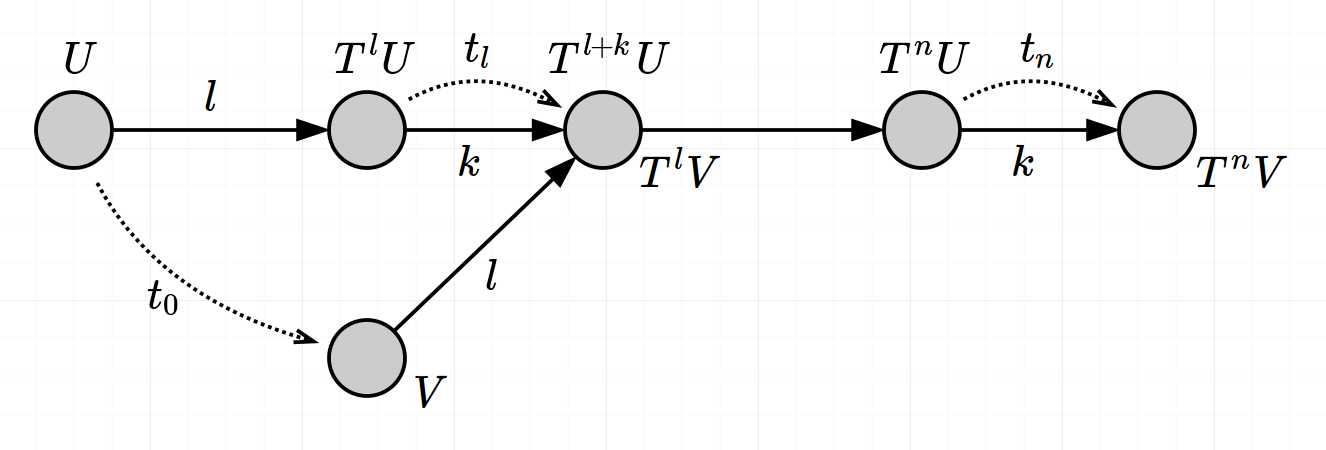
values at are involved). It is not difficult to see that the requirement that observes on in steps is equivalent to the condition . If the later is not the case, as , we can apply Theorem 2.1 to get a perturbation of such that . Define as
and on inductively as
One can check that is a perturbation of and that the -function associated to is precisely . Then, by Lemma 4.4, we can extend to a perturbation of , which will observe on in steps because . This proves that is dense. ∎
Definition 4.2.
Given a map and we define
The points will be called preperiodic points of period .
Lemma 4.7.
Let be a compact metric space and a continuous map. Let and be compact subsets with such that are pairwise disjoint, where . Suppose also that is injective on the sets . Then the set
is open and dense.
Proof.
Note that as then . Therefore is injective on the sets . This together with the injectivity assumptions on imply that restricts to homeomorphisms for and for .
Given let and be given by and . As we have
and then . As , by Proposition 4.2 we can perturb and to get and so that . Define by if and , and if and , where we write and . We have that is a perturbation of , where . Extend , applying Lemma 4.4, to a perturbation of . Then and, as , . Thus observes on in steps, because . We conclude that is dense. Finally, as is compact is open. ∎
Lemma 4.8.
Let be a second-countable space and a countable collection of subspaces of . Suppose that for every there exists and a relative neighborhood of . Then there exists a countable subcover of .
Proof.
For let and note that is a countable cover of . Let . Then is a cover of containing a neighborhood (in ) of every . As is Lindelöf, there exists a countable subcover of . Then is a countable subcover of . ∎
Proof of Theorem 2.3.
The general strategy of the proof is as follows. Let . For each we will find a set , relative neighborhood of in a subspace chosen from a fixed finite collection of subspaces of , satisfying that
is open an dense. Then, by Lemma 4.8, we can cover with countable many sets , say with . Therefore, as , we conclude that is a residual set.
Note that if for there exists a relative neighborhood as explained before then is a relative neighborhood in of satisfying the desired properties and vice versa. Then for each we need to take care only of one of the two points or , by adjoining subspaces to if necessary. That is, we can interchange and freely along the proof if needed.
For , we denote with
the -step orbit of and call length of the number
Given we distinguish six cases according to whether and meet or not, and to whether their lengths are equal or less than .
We enumerate the cases as in the following table. The remaining cases, corresponding to and , are reduced to the cases in the last two rows interchanging and .
| Case 1 | Case 2 | |
| Case 3 | Case 4 | |
| Case 5 | Case 6 |
Case 1: As in this case the -step orbits are disjoint, both of length , and is locally injective we can find compact neighborhoods and of and respectively, such that are pairwise disjoint and is injective when restricted to . Then, as and , we can apply Lemma 4.5 (with ) to conclude that is a neighborhood of (in the subspace ) for which is open an dense.
Case 2: In this case both -step orbits has length and meet. As we have , then and do not collapse in the same iterate, so we may suppose that are the first iterates of and that match, with . Then we are in the situation of Figure 2 with . \thisfloatsetupcapposition=beside, capbesideposition=right,center,floatwidth=.75capbesidewidth=.15
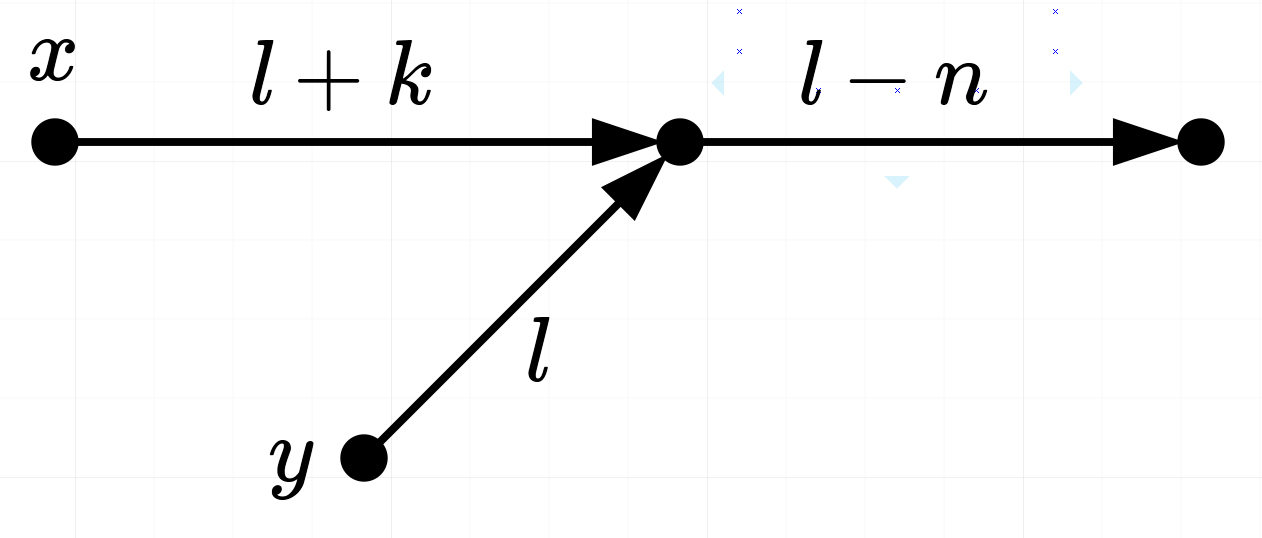
As is a locally injective map there exist compact neighborhoods and of and respectively, such that are pairwise disjoint with injective on these sets. Let , and . We have that and are compact, , are pairwise disjoint and is injective on these sets. Then, as , we can apply Lemma 4.6 (with ) to conclude that is a neighborhood of (in the subspace ) for which is open and dense. Finally, note that only finitely many subspaces are involved here because of the restrictions .
Case 3: In this case the -step orbits are disjoint, and . The last condition implies that with . As is a locally injective map we can take compact neighborhoods and of and respectively, such that are pairwise disjoint and is injective on these sets. Let and note that is compact. It is easily checked that the sets and are in the hypothesis of Lemma 4.7 (with ), being because and . Thus, is a neighborhood of (in the subspace ) for which is open and dense. Finally, observe that only finitely many subspaces are involved in this case because of the restrictions .
Cases 4 and 6: These cases are similar to Case 2. In these cases the -step orbits meet, and . As in the previous case, implies that is a preperiodic point, with . In addition, as the -step orbits meet, is also a preperiodic point of the same period, with . Thus both points and reach a common periodic orbit of period in and steps, respectively.
We discuss the subcases: (A) ; (B) .
Subcase A: In this subcase both orbits meet before they take a step in the common periodic orbit they reach. As in this case we have that because and do not collapse (). We may suppose that interchanging and if necessary. Let and () such that are the first iterates of and that match. From this point, say , there are steps to reach the periodic orbit () at a point that we call (), and then steps ahead along the periodic orbit until it closes (see Figure 3 (left)). Figure 3 (right) shows \thisfloatsetupfloatwidth=capbesidewidth=.15
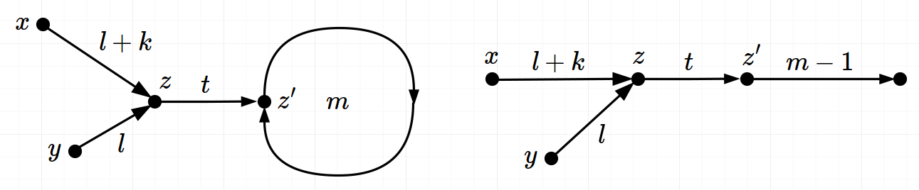
the situation we arrive after deleting the last step before the periodic orbit closes at (compare with Figure 2).
As is a locally injective map there exist compact neighborhoods and of and respectively, such that () are pairwise disjoint with injective on these sets. Let , and . We have that and are compact, , are pairwise disjoint and is injective on these sets. Then, as (because is homeomorphic to and ) we can apply Lemma 4.6 (with ) and conclude that is a neighborhood of (in the subspace ) for which is open and dense ().
Subcase B: In this subcase the orbits of and reach the common periodic orbit at different points and , respectively (Figure 4 (left)). \thisfloatsetupfloatwidth=capbesidewidth=.15
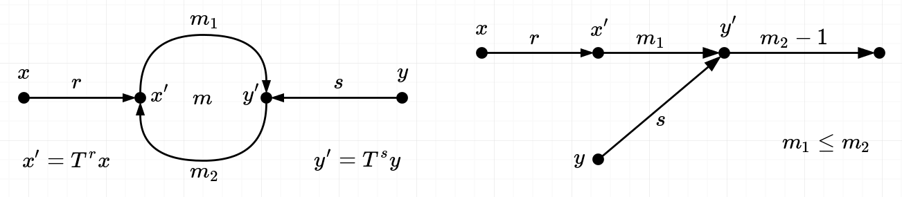
Let be the number of steps along the periodic orbit form to and number of steps from to (). We have or . Interchanging and if necessary we can suppose that we are in the second case. Deleting the step in which the periodic orbit closes at we arrive to the situation pictured in Figure 4 (right). Comparing with we have two cases: or ( and do not collapse). Suppose we have (the other case follows analogously). Let and such that and .
As is a locally injective map there exist compact neighborhoods and of and respectively, such that are pairwise disjoint with injective on these sets. Let , and . We have that and are compact, , are pairwise disjoint and is injective on these sets. As we can apply Lemma 4.6 (with ) and conclude that is a neighborhood of (in the subspace ) for which is open and dense ().
Finally, observe that in both subcases only finitely many subspaces are involved because of the restrictions , and .
Case 5: This case is similar to Case 3. In this case the -step orbits are disjoint and . The last condition implies that and with , and . As is locally injective there exist compact neighborhoods and of and respectively, such that are pairwise disjoint with injective on these sets. Let , and note that and are compact, with and similarly . Then we can apply Lemma 4.7 (with ) to conclude that is open and dense. Note that is a neighborhood of in the subspace . Again in this case, only finitely many subspaces are involved due to the restrictions on and . ∎