Simulating thimble regularization of lattice quantum field theories

Abstract:

Monte Carlo simulations of lattice quantum field theories on Lefschetz thimbles are non trivial. We discuss a new Monte Carlo algorithm based on the idea of computing contributions to the functional integral which come from complete flow lines. The latter are the steepest ascent paths attached to critical points, i.e. the basic building blocks of thimbles. The measure to sample is thus dictated by the contribution of complete flow lines to the partition function. The algorithm is based on a heat bath sampling of the gaussian approximation of the thimble: this defines the proposals for a Metropolis-like accept/reject step. The effectiveness of the algorithm has been tested on a few models, e.g. the chiral random matrix model. We also discuss thimble regularization of gauge theories, and in particular the successfull application to 0+1 dimensional QCD and the status and prospects for Yang-Mills theories.

1 Introduction

Following a seminal work by Witten [1], thimble regularization of lattice field theories has been in recent years introduced [2, 3]. In principle, it provides a very clean solution to the so-called sign problem. All in all, it amounts to deforming the original domain of integration of a given field theory into a new one, which is made by one or more thimbles. Thimbles are manifolds which live in the complexification of the original domain of integration. They are the union of the Steepest Ascent (SA) paths attached to critical points $\sigma$ of the (complexified) action. Thimbles have the same real dimension of the original manifold and on them the imaginary part of the action stays constant. The field theoretic quantities one is interested in are expressed as

$$\langle O\rangle=\frac{\sum_{\sigma}n_{\sigma}\,e^{-i\,S_{I}\left(p_{\sigma}\right)}\int_{\mathcal{J}_{\sigma}}\mathrm{d}y\,e^{-S_{R}}\,O\,e^{i\omega}}{\sum_{\sigma}n_{\sigma}\,e^{-i\,S_{I}\left(p_{\sigma}\right)}\int_{\mathcal{J}_{\sigma}}\mathrm{d}y\,e^{-S_{R}}\,e^{i\omega}}$$ (1)

where a positive measure $e^{-S_{R}}$ is in place and a constant phase $e^{-i\,S_{I}\left(p_{\sigma}\right)}$ has been factored out of the integral. In the previous formula the denominator reconstructs the partition function $Z$. A so-called residual phase $e^{i\omega}$ is there that accounts for the relative orientation between the canonical complex volume form and the real volume form, characterizing the tangent space of the thimble.
While the solution to the sign problem via a deformation of the integration domain is powerful and conceptually satisfying, thimbles are non-trivial manifolds, for which a local characterisation is missing. In particular, devising Monte Carlo methods to sample integrals on thimbles is a delicate issue.

2 A new algorithm for thimble regularization

A simple way to characterise points on a thimble goes through a constructive approach. Given a critical point of the (complexified) action $S$, one can determine the tangent space to the thimble at that critical point. This is done by performing the Takagi factorization of the Hessian of the action $S$ at the critical point: one is left with Takagi values ${\lambda_{i}>0}$ and Takagi vectors $v^{(i)}$, which are a basis of the tangent space. The tangent space contains all the directions along which the SA paths defined by

$$\frac{d}{dt}z_{i}=\frac{\partial\bar{S}}{\partial\bar{z}^{i}}$$ (2)

leave the critical point. If we impose a normalization condition

$$\sum_{i=1}^{n}n_{i}^{2}=\mathcal{R}$$

all those directions are mapped to vectors

$$\sum_{i=1}^{n}n_{i}v^{(i)}.$$

It is thus quite natural to single out any given point on a thimble by the correspondence

$$\mathcal{J}_{\sigma}\ni z\leftrightarrow\left(\hat{n},t\right)\in S^{n-1}_{\mathcal{R}}\times\mathbb{R}$$ (3)

with $S^{n-1}_{\mathcal{R}}$ the $(n-1)$-sphere of radius $\sqrt{\mathcal{R}}$. In [4] we made use of this approach to solve a Chiral Random Matrix Model by means of thimble regularization. It turns out that (3) amounts to computing a Jacobian just like in the Faddeev-Popov approach to gauge fixing. For the sake of simplicity we restrict the discussion to cases in which the contribution attached to a single critical point $\sigma$ reconstructs the entire functional integral (this happened to hold for the problem discussed in [4], where however we discussed how to proceed in a generic case). Let us define

$$Z_{\sigma}=\int\limits_{\mathcal{J}_{\sigma}}\mathrm{d}^{n}y\,e^{-S_{R}}$$ (4)

With a slight abuse of terminology we will refer to this expression as a partition function. All in all, it can be rewritten

$$Z_{\sigma}=\int\mathcal{D}\hat{n}\,Z_{\hat{n}}$$ (5)

with the measure over $S^{n-1}_{\mathcal{R}}$

$$\mathcal{D}\hat{n}\equiv\prod_{k=1}^{n}\mathrm{d}n_{k}\delta\left(\left|\vec{n}\right|^{2}-\mathcal{R}\right)$$

and the partial partition function

$$Z_{\hat{n}}=\int\limits_{-\infty}^{+\infty}\mathrm{d}t\,\Delta_{\hat{n}}(t)\,e^{-S_{R}(\hat{n},t)}.$$ (6)

The partition function has been decomposed in contributions $Z_{\hat{n}}$ attached to SA paths (aka complete flow lines) and $\Delta_{\hat{n}}(t)$ can be thought of as an extra contribution to the measure (on top of $e^{-S_{R}(\hat{n},t)}$) along the SA defined by the direction $\hat{n}$. The computation of $\Delta_{\hat{n}}(t)$ requires that one parallel transports the basis of the tangent space at the critical point along the flow, to have a basis $\{V^{(i)}\}$ at the (generic) point associated to the flow time $t$. More precisely, by assembling the $V^{(i)}$ into the matrix $V$, one finds that

$$Z_{\hat{n}}=2\sum_{i=1}^{n}\lambda_{i}n_{i}^{2}\int\limits_{-\infty}^{+\infty}\mathrm{d}t\,e^{-S_{\mathrm{eff}}(\hat{n},t)}$$ (7)

where the ${\lambda_{i}>0}$ are the Takagi values that were mentioned above and the effective action $S_{\mathrm{eff}}$ is given by

$$S_{\mathrm{eff}}(\hat{n},t)=S_{R}(\hat{n},t)-\log\left|\det V(t)\right|.$$ (8)

In the (simplified) framework we are studying (a single contribution to (1), coming from one thimble), it is easy to see that the computation of (1) simply amounts to

$$\langle O\rangle=\frac{\langle O\,e^{i\,\omega}\rangle_{\sigma}}{\langle e^{i\,\omega}\rangle_{\sigma}}$$ (9)

where a reweighting with respect to the critical phase is in place and we introduced the notation

$$\langle\ldots\rangle_{\sigma}=\frac{\int\limits_{\mathcal{J}_{\sigma}}\mathrm{d}^{n}y\,\ldots\,e^{-S_{R}}}{\int\limits_{\mathcal{J}_{\sigma}}\mathrm{d}^{n}y\,e^{-S_{R}}}.$$

Making use of the representation (3), and thus of the same notation in which we wrote (5) and (6), one can now rephrase

$$\langle f\rangle_{\sigma}=\frac{1}{Z_{\sigma}}\int\limits_{\mathcal{J}_{\sigma}}\mathrm{d}^{n}y\,f\,e^{-S_{R}}=\frac{1}{Z_{\sigma}}\int\mathrm{D}\hat{n}\;(2\sum_{i=1}^{n}\lambda_{i}n_{i}^{2})\int\limits_{-\infty}^{+\infty}\mathrm{d}t\,f(\hat{n},t)\,e^{-S_{\mathrm{eff}}(\hat{n},t)}=\int\mathrm{D}\hat{n}\,\frac{Z_{\hat{n}}}{Z_{\sigma}}\,f_{\hat{n}}$$ (10)

in which

$$f_{\hat{n}}\equiv\frac{1}{Z_{\hat{n}}}(2\sum_{i=1}^{n}\lambda_{i}n_{i}^{2})\int\limits_{-\infty}^{+\infty}\mathrm{d}t\,f(\hat{n},t)\,e^{-S_{\mathrm{eff}}(\hat{n},t)}$$

almost looks like a functional integral along a single complete flow line. (10) can be put at work in the computation of (9) (with $f=O\,e^{i\,\omega}$ in the numerator and $f=e^{i\,\omega}$ in the denumerator). It is interesting to notice that the $\frac{Z_{\hat{n}}}{Z_{\sigma}}$ factor contained in (10) is a legitimate (well normalized) weight, so that (10) is nothing but the average of the $f_{\hat{n}}$, i.e. the average of the contributions that a given observable takes from complete flow lines. This average is computed in a given normalization, fixed by the $\frac{Z_{\hat{n}}}{Z_{\sigma}}$ weight, which in turn represents the fraction of the partition function which is provided by a single complete flow line. In [4] we made use of this approach for the computation of (9), but we made no attempt at implementing importance sampling with respect to the $\frac{Z_{\hat{n}}}{Z_{\sigma}}$ weight: computations were simply performed by flat, crude Monte Carlo, i.e. extracting the directions $\hat{n}$ (flat) randomly.
Here we present a dynamic Monte Carlo, i.e. one performing importance sampling. This will amount to extract directions according to the probability $P(\hat{n})=\frac{Z_{\hat{n}}}{Z_{\sigma}}$. We proceed as follow. In our Markov chain we start from the current configuration (i.e. a direction $\hat{n}$) and we propose a new one (i.e. a direction $\hat{n}^{\prime}$) which is identical to $\hat{n}$ apart from two randomly chosen components, say $(n_{i},n_{j})$ with $i\neq j$. We define $C$ by

$$C\equiv n_{i}^{2}+n_{j}^{2}=\mathcal{R}-\sum_{k\neq i,j}n_{k}^{2}$$

which is fixed by the normalization $\left|\vec{n}\right|=\sqrt{\mathcal{R}}$ and by the values of all $\{n_{k}\}_{k\neq i,j}$. It exists a coordinate system in which we can now parametrize all the new values for $(n_{i},n_{j})$ by

$$n_{i}=\sqrt{C}\,\cos\phi\;\;\;\;\;n_{j}=\sqrt{C}\,\sin\phi$$

with $\phi\in[0,2\pi)$, and our aim is therefore to extract a value for $\phi$. We now define a gaussian thimble: it is the thimble associated to a critical point of an action which only has quadratic fluctuations on top of the value at that critical point. It is easy to find out that it is a flat thimble, and for it one can compute

$$Z^{\mathcal{G}}_{\hat{n}}=2\sum_{i=1}^{n}\lambda_{i}n_{i}^{2}\int\limits_{-\infty}^{+\infty}\mathrm{d}t\,e^{\;\;\sum\limits_{i=1}^{n}\lambda_{i}\,t-\frac{1}{2}\sum\limits_{i=1}^{n}\lambda_{i}n_{i}^{2}e^{2\lambda_{i}t}}.$$ (11)

We now evaluate (11) for $\hat{n}^{\prime}$ as a function of $\phi$ and define the cumulative distribution function

$$F^{\mathcal{G}}_{\hat{n}^{\prime}}(\phi)\equiv\frac{\int\limits_{0}^{\phi}\mathrm{d}\varphi\,Z^{\mathcal{G}}_{\hat{n}^{\prime}(\varphi)}}{\int\limits_{0}^{2\pi}\mathrm{d}\varphi\,Z^{\mathcal{G}}_{\hat{n}^{\prime}(\varphi)}}.$$

By extracting $\xi\in[0,1]$ uniformly distributed and computing $\phi=F^{\mathcal{G}-1}_{\hat{n}^{\prime}}(\xi)$, we obtain a $\phi$ (i.e. a $\hat{n}^{\prime}$) that is distributed according to $P(\phi)\propto Z_{\hat{n}^{\prime}(\phi)}$. We now accept the proposed configuration with the standard Metropolis test

$$P_{\mathrm{acc}}\left(\hat{n}^{\prime}\bigr{|}\hat{n}\right)=\min\left\{1,\frac{Z_{\hat{n}^{\prime}}}{Z_{\hat{n}}}\frac{Z^{\mathcal{G}}_{\hat{n}}}{Z^{\mathcal{G}}_{\hat{n}^{\prime}}}.\right\}$$ (12)

This method turns out to be quite effective. In Figure 1 we present results for the Chiral Random Matrix Model of [4]. For a given value of the mass parameter ($m=8$) we compare the results for the relevant condensate as computed from the crude Monte Carlo and as computed from the new importance sampling method. Errorbars are comparable despite the huge difference in the number of sampled configurations. At a lower value of the mass parameter ($m=7$), it turns out that crude Monte Carlo does not converge, while the new method gets the correct result.

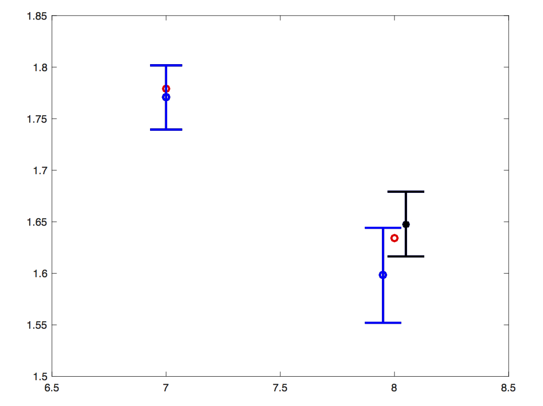
Figure 1: Computation of an observable (chiral condensate) of a Chiral Random Matrix Theory via crude or dynamic Monte Carlo for different values of a mass parameter $m$. At $m=8$ the dynamic Monte Carlo obtains the result to the left, despite this comes from sampling $1300$ configurations, vs the $22000$ configurations sampled by crude Monte Carlo (result to the right). At $m=7$ crude Monte Carlo does not even converge, while dynamic gets the correct result.

3 0+1 dim QCD

We made use of the formulation induced by (3) also for 0+1 dimensional QCD [5]. As it is well known, this theory is in a convenient gauge reduced to a single integral over $SU(3)$

$$Z_{N_{f}}=\int\limits_{\mathrm{SU}(3)}\mathrm{d}U\,{\det}^{N_{f}}\left(A\,\mathds{1}_{3\times 3}+e^{\mu/T}U+e^{-\mu/T}U^{\dagger}\right)$$ (13)

The thimble machinery for $SU(N)$ was described in [6], to which we refer the interested reader. Here the point we want to make is that three critical points are there: does one need to take into account all of them? This would contradict the hypothesis of the main thimble dominance (notice that however this hypothesis is supposed to hold at most in a thermodynamic limit we are quite apart from in this system). The answer is illustrated in Figure 2. On the left, we plot the (log of) the ratio between the partition functions (4) computed on the thimbles attached to the non-trivial elements of $Z_{3}$ (they are equal) and the one computed on the thimble attached to the identity, as computed in a semi-classical approximation. The result is interesting. While the complete analytic result does not know anything about thimbles, the semi-classical one attaches a different value to the computation in the background of each critical point. Results are for $N_{f}=2$ and $m=1$ and different values of the ratio $\frac{\mu}{T}$. One can clearly notice that at certain values of $\frac{\mu}{T}$ the contributions from thimbles other than the identity are supposed to give a sizable contribution. On the right one finds out that this is indeed the case. Different symbols in the computation of the trace of Polyakov (second line) and anti-Polyakov loop (third line) refer to computations performed only keeping into account the identity: they clearly miss the correct results.

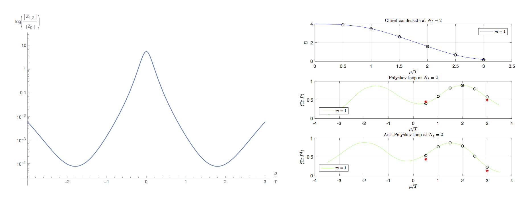
Figure 2: Thimble computation of 0+1-dimensional QCD (see text).

4 First steps in Yang-Mills theories

We finally give a rough account of our first tests on Yang-Mills (YM) theories. Again, the reader is referred to [6] for the relevant formalism. The theory at hand is the standard Yang-Mills Wilson action, with a sign problem which is forced by plugging in a complex value for the coupling $\beta$. Results can be tested versus analytic ones in $d=2$. We tried to test in this framework the viability of what we call the gaussian approximation. This could be seen successfully at work in [7] (but see also comments in [4]). It amounts to performing a Langevin simulation on the thimble. The drift term makes the system stay on the thimble by very definition, and the problem is reduced to sample the noise term on the tangent space. A solution was put forward in [2]. In the gaussian approximation one simply projects the noise over the tangent space at the critical point, thus assuming the flat thimble to be a reasonable deformation of both the original domain of integration and/or of the actual thimble. One does not obtain a constant imaginary part of the action, but fluctuations are typically (even very) mild, at most asking for a (viable) reweighting. Figure 3 displays gaussian approximation results for the action density of a $SU(2)$ YM theory in $d=2$ on a (ridiculous…) $4^{2}$ lattice at $\beta=5e^{i0.2}$. At this value of the coupling semi-classical results would suggest the gaussian approximation to work fairly well. This is indeed the case. In particular numerical (gaussian approximation) results miss the analytic result without reweighting for the imaginary part of the action (left), while a correct result is got once reweighting is plugged in. All this is very preliminary. Still it is a very first example of thimble regularization for gauge thoeries.

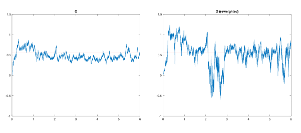
Figure 3: Computation of the action density for $SU(2)$ YM theory in $d=2$ on a $4^{2}$ lattice at $\beta=5e^{i0.2}$. Red lines display the analytic result. On the left there is no reweighting for the imaginary part of the action, which is instead there on the right. The correct result is got in the latter case, despite quite sizable fluctuations (notice the different scales for $y$-axis).

References

- [1] E. Witten, Analytic Continuation Of Chern-Simons Theory, AMS/IP Stud. Adv. Math. 50 (2011) 347
- [2] M. Cristoforetti et al. [AuroraScience Collaboration], New approach to the sign problem in quantum field theories: High density QCD on a Lefschetz thimble, Phys. Rev. D 86 (2012) 074506
- [3] H. Fujii, D. Honda, M. Kato, Y. Kikukawa, S. Komatsu and T. Sano, Hybrid Monte Carlo on Lefschetz thimbles - A study of the residual sign problem, JHEP 1310 (2013) 147
- [4] F. Di Renzo and G. Eruzzi, Thimble regularization at work: from toy models to chiral random matrix theories, Phys. Rev. D 92 (2015) 085030
- [5] N. Bilic and K. Demeterfi, One-dimensional QCD With Finite Chemical Potential, Phys. Lett. B 212, 83 (1988).
- [6] F. Di Renzo and G. Eruzzi, Thimble regularization at work for Gauge Theories: from toy models onwards, PoS LATTICE 2015 (2016) 189
- [7] M. Cristoforetti, F. Di Renzo, A. Mukherjee and L. Scorzato, Monte Carlo simulations on the Lefschetz thimble: Taming the sign problem, Phys. Rev. D 88 (2013) 051501