Stochastic study of information transmission and population stability in a generic bacterial two-component system

Abstract

Studies on the role of fluctuations in signal propagation and on gene regulation in monoclonal bacterial population have been extensively pursued based on the machinery of two-component system. The bacterial two-component system shows noise utilisation through its inherent plasticity. The fluctuations propagation takes place using the phosphotransfer module and the feedback mechanism during gene regulation. To delicately observe the noisy kinetics the generic cascade needs stochastic investigation at the mRNA and protein levels. To this end, we propose a theoretical framework to investigate the noisy signal transduction in a generic bifunctional two-component system. The model shows reliability in information transmission through quantification of several statistical measures. We further extend our analysis to observe the protein distribution in a population of cells. Through numerical simulation, we identify the regime of the kinetic parameter set that generates a stability switch in the steady state distribution of proteins. The results of our theoretical analysis show key features of the network. The noise permeation and information propagation in the autoregulation module is feeble. However, the phosphotransfer module compensates such weakness and plays a significant role in information transmission. The bimodality due to fluctuations pampers the emergence of persistence in an isogenic bacterial pool.

I Introduction

To deal with fluctuations in biological systems is highly motivating because nature is fundamentally noisy in nature Balázsi et al. (2011); Raj and van Oudenaarden (2008); Eldar and Elowitz (2010). The interplay between deterministic and random processes configures the pool of different biological entities along with the adoption of several survival strategies. Also, the phenotypic heterogeneity brings in uniqueness to an individual in a population Davidson and Surette (2008). This happens not only for differences at the genetic level but due to the presence of noise in an isogenic population. Although genetic diversity is decisive in favour of evolution in the environmental and historical variability, the phenotypic variety can be ascribed to the randomness, intrinsic and extrinsic. Cells, being exposed to the diverse environment, must respond to the fluctuating external signal to control their fate Tsimring (2014).

A two-component system (TCS) is the most ubiquitous and the most compact signal transduction machinery observed in bacteria and in some plants and fungi Laub and Goulian (2007); Goulian (2010); Groisman (2016). The TCS is a type of phosphotransfer cascade like the MAPK cascade, but differs in the molecular mechanism Stock et al. (2000). In TCS, only one molecule of ATP is consumed and gets transferred through the cascade, whereas in the case of MAPK, at every phosphorylation step ATP is consumed. The TCS is composed mainly of two parts: A membrane-bound sensor kinase (SK) protein, and a cytoplasmic response regulator (RR) protein. The RR protein, activated by the phosphorylation, acts as a transcription factor for downstream genes or facilitates another target like flagellar locomotive switch Micali and Endres (2016). The simplest and modular TCS, which are efficiently present in the broad spectrum of efficacy, overtake popularity than other signal transduction motifs due to its inherent plasticity in noise regulation. Earlier studies on functionality of the SK Maity et al. (2014); Ortega et al. (2002); Yang et al. (2015), input-output robustness of the phosphotransfer module Shinar et al. (2007); Batchelor and Goulian (2003), bistability due to TCS mediated gene regulation Igoshin et al. (2008); Ghosh et al. (2011); Hoyle et al. (2012), different stochastic switching responses Kierzek et al. (2010) and stochasticity induced active state locking and growth-rate dependent bistability Wei et al. (2014) have been reported. Although most of the reported TCS have an autoregulatory feature, the know-how of noisy gene regulation coupled with the TCS signaling pathway has not been explored till date. Within the purview of single-cell scenario, the effect of fluctuations can not be neglected in the TCS signaling pathway as fluctuations, whatever may be its source, has a key role in the gene regulation as well as in the post-translational modification that is taking place in the noisy cellular environment Sanchez and Kondev (2008). In the present study, our prime interest is to quantify fluctuations in the TCS that has a feedback in the form of autoregulation at the operon of the two proteins, the sensor kinase and the response regulator. Depending on the nature of fluctuations of the extracellular signal, the signaling cascade must orient itself as to sense and respond appropriately. To this end, the phosphorylated response regulator ($R_{P}$) is considered as the output of the network. Hence, to study the propagation of noise through the cascade, we need to quantify the noisy characteristics of $R_{P}$ due to the external signal, the inducer ($I$). In this paper, we compute several experimentally realisable quantities, viz., variance, Fano factor, etc. We also calculate the information processing through the network as TCS transmits information of the alteration of the environment.

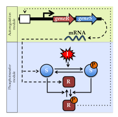
Figure 1: (color online) The two-component system. Schematic diagram of a generic two-component system composed of the phosphotransfer and the autoregulation module. The red asteroid shows external inducer $I$. The blue sphere stands for the sensor kinase, $S$. Similarly, the brown box represents the response regulator, $R$. $P$ in orange sphere stands for the phosphate group. The wavy blue line is for the mRNA generated from the operon. The solid lines with arrowhead stands for phosphotranfer kinetics. The dashed lines takes care of both transcription and subsequent translation. The dotted line represents the positive feedback on the operon.

In the last section of the paper, we present a population switch that makes transition from bistable to monostable state and vice versa. Bistability is a widely observed phenomenon in biochemical networks with sufficient nonlinearity Tiwari et al. (2011). In the case of deterministic systems, with weak nonlinearity, bistability can not be observed. However, if one goes for small reaction volume, the generated stochasticity may induce bistability Friedman et al. (2006); Bishop and Qian (2010). Nowadays with the increased use of the methods like fluorescence microscopy and flow cytometry, one may decipher the noise induced heterogeneity in a clonal population Raj and van Oudenaarden (2008); Spiller et al. (2010). The advantage of a microscopic stochastic study over the macroscopic deterministic observation is that the same mathematical construct of a TCS network shows monostable as well as bistable property depending on the system size. Bistable switches do not have any clue of the genetic changes, hence they are epigenetic. Bistability has been observed in E. coli by persister cells and in B. subtilis through spore formation and cannibalism Dubnau and Losick (2006). But the mechanism is different for the two species. The first one happens due to positive autoregulation of the master gene. In the second one, there exist a pair of mutual repressors. In the current model, we are interested in the first type, positive autoregulation driven bistability. To this end, we examine the TCS dynamics using a stochastic approach for a range of parameter set to observe the transition from unimodal to a bimodal distribution.

II The Model

The system, here we are dealing with, is a generic bacterial two-component signal transduction machinery that gets activated by an external stimulus. While activated, it regulates one or several downstream genes. The full signal transduction pathway may be divided into two interconnected modules, the autoregulation module and the phosphotransfer module. The autoregulation module is driven by the latter. In the phosphotransfer module, the external stimulus or the inducer $I$ triggers the autophosphorylation of the membrane-bound sensor kinase (SK) $S$ at the conserved Histidine residue to produce the phosphorylated form of $S$, $S_{P}$. The phosphate group is then transferred to the Aspartate domain of the cognate cytoplasmic response regulator (RR) $R$ via a phosphotransfer mechanism along with the formation of $R_{P}$. Once produced $R_{P}$ regulates the binding of RNA polymerase to the DNA of several downstream genes. In addition, it regulates the activity of its operon present in the autoregulation module (see Fig. 1). The phosphorylated RR becomes dephosphorylated by the unphosphorylated SK, thus acting as a phosphatase. The ability of the SK to act as kinase as well as phosphatase assigns it a bifunctional characteristic Laub and Goulian (2007); Tiwari et al. (2010) and allows one to place it in a broad category of functional motifs, the paradoxical components Hart and Alon (2013). For a bifunctional TCS SK can thus act as a source and a sink of the phosphate pool. The relevant kinetics of the full network along with the kinetic rate parameters are tabulated in Table 1. At this point it is important to mention that, in certain TCS, the phosphatase activity of the sensor kinase is absent thus making the TCS monofunctional Laub and Goulian (2007).

To incorporate fluctuations due to different noise processes, we opt for Langevin method and calculate various physical entities. The extracellular noise comes from the environmental stimulus $I$. On the other hand, the gene regulation and the post-translational modification contribute to the intracellular noise. The Langevin equation of the inducer can be written as

$$\frac{dI}{dt}=k_{sI}-k_{dI}I+\xi_{I},$$ (1)

with $\langle\xi_{I}(t)\rangle=0$, $\langle\xi_{I}(t)\xi_{I}(t+\tau)\rangle=(k_{sI}+k_{dI}\langle I\rangle)\delta(\tau)=2k_{dI}\langle I\rangle\delta(\tau)$. Here $\langle I\rangle$ is the mean (ensemble average) inducer level at steady state. $\xi_{I}$ is the extracellular fluctuations incorporated by the external stimulus. The phosphotransfer reaction kinetics shown in Table I with the associated stochasticity can be expressed as

$$\frac{dS_{P}}{dt} = k_{ap}I(S_{T}-S_{P})-k_{adp}S_{P}-k_{k}S_{P}(R_{T}-R_{P})$$ (2)

$$-k_{dp}S_{P}+\xi_{S_{P}},$$

$$\frac{dR_{P}}{dt} = k_{k}S_{P}(R_{T}-R_{P})-k_{p}R_{P}(S_{T}-S_{P})$$ (3)

$$-k_{dp}R_{P}+\xi_{R_{P}},$$

where $S_{T}$, $S_{P}$, $R_{T}$ and $R_{P}$ are the pool of total and phosphorylated form of $S$ and $R$ respectively. We note that while writing Eqs. (2-3) we consider simple bimolecular kinetics instead of Michaelis-Menten kinetics. This is a valid approximation as long as the Michaelis-Menten complex are low in concentration. Also, consideration of bimolecular kinetics makes our subsequent analytical calculation tractable. As a result, $S(t)+S_{P}(t)=S_{T}(t)$ and $R(t)+R_{P}(t)=R_{T}(t)$, which we have used while writing Eqs. (2-3). Here, $S_{T}(t)$ and $R_{T}(t)$ are not constant quantity, rather they keep on changing with time and only reach a constant value at steady state for a fixed value of inducer level. The $R_{P}$ mediated transcription and the expression kinetics of the two different pools of proteins (SK and RR) is formulated as follows

$$\frac{dm}{dt} = k_{sm}f(R_{P})-k_{dm}m+\xi_{m},$$ (4)

$$\frac{dS_{T}}{dt} = k_{ss}m-k_{dp}S_{T}+\xi_{S_{T}},$$ (5)

$$\frac{dR_{T}}{dt} = k_{sr}m-k_{dp}R_{T}+\xi_{R_{T}}.$$ (6)

Here $f(R_{P})=R_{P}/(R_{P}+K)$, $K$ is the dissociation constant. $\xi_{m}$ is the transcriptional noise associated with the synthesis and degradation of mRNA, $m$. $\xi_{S_{T}}$ and $\xi_{R_{T}}$ are translational noise. The additive noise terms $\xi_{S_{P}}$, $\xi_{R_{P}}$, $\xi_{m}$, $\xi_{S_{T}}$ and $\xi_{R_{T}}$ take care of fluctuations in the copy number of $S_{P}$, $R_{P}$, $m$, $S_{T}$ and $R_{T}$, respectively. The noise terms are independent and Gaussian distributed with the statistical properties Maity et al. (2014); Elf and Ehrenberg (2003); Swain (2004); Paulsson (2004); Tǎnase-Nicola et al. (2006); Warren et al. (2006); van Kampen (2007); Mehta et al. (2008); Maity et al. (2015); Grima (2015); Biswas and Banik (2016) $\langle\xi_{S_{P}}(t)\rangle=\langle\xi_{R_{P}}(t)\rangle=\langle\xi_{m}(t)\rangle=\langle\xi_{S_{T}}(t)\rangle=\langle\xi_{R_{T}}(t)\rangle$ $=0$ and

$$\langle\xi_{S_{P}}(t)\xi_{S_{P}}(t+\tau)\rangle = 2k_{ap}[\langle S_{T}\rangle-\langle S_{P}\rangle]\langle I\rangle\delta(\tau),$$

$$\langle\xi_{R_{P}}(t)\xi_{R_{P}}(t+\tau)\rangle = 2k_{k}\langle S_{P}\rangle[\langle R_{T}\rangle-\langle R_{P}\rangle]\delta(\tau),$$

$$\langle\xi_{m}(t)\xi_{m}(t+\tau)\rangle = 2k_{dm}\langle m\rangle\delta(\tau),$$

$$\langle\xi_{S_{T}}(t)\xi_{S_{T}}(t+\tau)\rangle = 2k_{dp}\langle S_{T}\rangle\delta(\tau),$$

$$\langle\xi_{R_{T}}(t)\xi_{R_{T}}(t+\tau)\rangle = 2k_{dp}\langle R_{T}\rangle\delta(\tau).$$

The cross-correlation between $\xi_{S_{P}}$ and $\xi_{R_{P}}$ arises naturally due to kinetics shown by Eqs. (2-3) Maity et al. (2014); Swain (2004); Tǎnase-Nicola et al. (2006),

$$\langle\xi_{S_{P}}(t)\xi_{R_{P}}(t+\tau)\rangle=-k_{k}\langle S_{P}\rangle[\langle R_{T}\rangle-\langle R_{P}\rangle]\delta(\tau).$$

Here, $\langle\cdots\rangle$ represents ensemble average evaluated at steady state. While writing the noise correlation in the present work we have used constant noise intensity evaluated at steady state, an approximation, that makes the following analytical calculation tractable. Linearization of Eq. (1) and Eqs. (2-6) around the mean value at steady state, i.e., $I=\langle I\rangle+\delta I$, $S_{P}=\langle S_{P}\rangle+\delta S_{P}$, $R_{P}=\langle R_{P}\rangle+\delta R_{P}$, $m=\langle m\rangle+\delta m$, $S_{T}=\langle S_{T}\rangle+\delta S_{T}$ and $R_{T}=\langle R_{T}\rangle+\delta R_{T}$ yields

$$\frac{d}{dt}\mathbf{\delta X(t)}=\mathbf{J}_{X=\langle X\rangle}\mathbf{\delta X(t)}+\mathbf{\Xi(t)}.$$ (7)

Here, $\mathbf{\delta X}$ is the fluctuations matrix. $\mathbf{\Xi}$ and $\mathbf{J}$ are the noise matrix and the Jacobian matrix of the averages evaluated at steady state, respectively (see Appendix for explicit form of the matrices). To solve Eq. (7) we write the Lyapunov equation at steady state Elf and Ehrenberg (2003); Paulsson (2004); van Kampen (2007); Keizer (1987); Paulsson (2005); Gardiner (2009); Grima et al. (2011)

$$\mathbf{J}\mathbf{\sigma}+\mathbf{\sigma}\mathbf{J}^{T}+\mathbf{D}=0,$$ (8)

where $\mathbf{\sigma}$ is the covariance matrix and $\mathbf{D}=\langle\mathbf{\Xi\Xi}^{T}\rangle$ is the diffusion matrix (see Appendix). To quantify all the network properties and the information transmission, we solve the Lyapunov equation (8) and evaluate the elements of the covariance matrix $\mathbf{\sigma}$

$${\bf\sigma}=\left(\begin{array}[]{cccccc}\sigma^{2}_{I}&\sigma^{2}_{IS_{P}}&\sigma^{2}_{IR_{P}}&\sigma^{2}_{Im}&\sigma^{2}_{IS_{T}}&\sigma^{2}_{IR_{T}}\\ \sigma^{2}_{S_{P}I}&\sigma^{2}_{S_{P}}&\sigma^{2}_{S_{P}R_{P}}&\sigma^{2}_{S_{P}m}&\sigma^{2}_{S_{P}S_{T}}&\sigma^{2}_{S_{P}R_{T}}\\ \sigma^{2}_{R_{P}I}&\sigma^{2}_{R_{P}S_{P}}&\sigma^{2}_{R_{P}}&\sigma^{2}_{R_{P}m}&\sigma^{2}_{R_{P}S_{T}}&\sigma^{2}_{R_{P}R_{T}}\\ \sigma^{2}_{mI}&\sigma^{2}_{mS_{P}}&\sigma^{2}_{mR_{P}}&\sigma^{2}_{m}&\sigma^{2}_{mS_{T}}&\sigma^{2}_{mR_{T}}\\ \sigma^{2}_{S_{T}I}&\sigma^{2}_{S_{T}S_{P}}&\sigma^{2}_{S_{T}R_{P}}&\sigma^{2}_{S_{T}m}&\sigma^{2}_{S_{T}}&\sigma^{2}_{S_{T}R_{T}}\\ \sigma^{2}_{R_{T}I}&\sigma^{2}_{R_{T}S_{P}}&\sigma^{2}_{R_{T}R_{P}}&\sigma^{2}_{R_{T}m}&\sigma^{2}_{R_{T}S_{T}}&\sigma^{2}_{R_{T}}\end{array}\right)$$

The elements of $\mathbf{\sigma}$ are the variance and covariances of the subscripted quantities.

For numerical validation of the results calculated analytically, we adopt stochastic simulation algorithm (SSA) Gillespie (1976, 1977). The kinetics and propensity associated with each chemical reaction are tabulated in Table 1. The simulation results presented in the following section are average of $10^{6}$ independent trajectories. During simulation, each independent run starts with a constant pool of $S$ and $R$ that takes care of basal level of the two proteins. In the absence of the stimulus $I$ ($k_{s}=0$), only the degradation of $S$ and $R$ are operative along with the constant pool of the same. In such situation, the concentration of proteins goes down to zero at steady state. Once the inducer assumes a non-zero value ($k_{s}\neq 0$) it activates the phosphotransfer cascade and generates the pool of the transcription factor $R_{P}$, thus providing a positive feedback on the operon. As a result, the full signaling network (autoregulation+phosphotransfer) becomes operative.

III Results and Discussions

The utility of the TCS is to respond rapidly by properly transducing an external signal. The response, here we are dealing with, is the transcriptional autoregulation at the operon of SK and RR along with other downstream genes by the phosphorylated response regulator $R_{P}$. The pool of $R_{P}$ in turn gets accumulated by the inducer mediated autophosphorylation and subsequent phosphotransfer of the sensor kinase $S_{P}$. The stochastic fluctuations can be calculated through different statistical measures for the current model. As $R_{P}$ is considered as the output of the full TCS, the common measures of fluctuations, like variance, Fano factor are observed for $R_{P}$. The fidelity or the reliability of the present signaling cascade can be also measured in terms of mutual information, network gain and intrinsic noise. From the biological outlook, the sources of different noise processes are widespread inside and outside the cell. Some sources of randomness are shared by different proteins, correlated through interaction in the post-translational modification or due to sharing common expression operon. If we observe the post-translational reactions like the phosphotransfer between $S$ and $R$, the source of the fluctuations may differ from that of the gene regulation. Here, to quantify all the network properties, we propose the inducer, $I$ to be the input and $R_{P}$ to be the network output as $R_{P}$ being of prime interest since it regulates many of the downstream genes. The classification of the source of noise is difficult for such a large and modular network. But one can quantify the fluctuations through the aforesaid different measures.

The entire observation in this paper is partitioned into four segments. First, we focus on the phosphotransfer module to quantify fluctuations over a range of the external signal $I$. Second, we concentrate on the stochastic transcriptional process, which shows the dynamics of mRNA fluctuations in response to the signal mediated feedback of the response regulator. Third, we focus on the entire network to decipher different stochastic network properties, which reflect the reliability of the network performance. The final segment deals with the phosphorylated response regulator distribution at steady state to find the role of the switch in characterising the stability at the steady state.

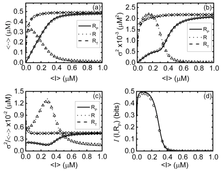
Figure 2: Fluctuations in response regulator. Different statistical measures for the pool of response regulator. The lines indicate the theoretical values of $R_{P}$ (solid), $R$ (dotted) and $R_{T}$ (dashed) and the symbols stand for the numerical values of $R_{P}$ (circle), $R$ (triangle) and $R_{T}$ (diamond). (a) averages ($\langle R_{P}\rangle,\langle R\rangle,\langle R_{T}\rangle$), (b) variances ($\sigma^{2}_{R_{P}},\sigma^{2}_{R},\sigma^{2}_{R_{T}}$) and (c) Fano factors ($\sigma^{2}_{R_{P}}/\langle R_{P}\rangle,\sigma^{2}_{R}/\langle R\rangle,\sigma^{2}_{R_{T}}/\langle R_{T}\rangle$) are plotted as a function of average signal strength $\langle I\rangle$. The mutual information ${\cal I}(I,R_{P})$ between the the input signal $I$ and the output $R_{P}$ is shown in (d). The symbols are generated using stochastic simulation algorithm Gillespie (1976, 1977) and the lines are due to theoretical expressions.

III.1 Fluctuations in the protein pool

While sensing the external stimulus $I$, $S$ gets itself phosphorylated and triggers the flow of signal. During phosphotransfer to $R$ through the kinase activity, $S_{P}$ transmits the noisy signal to the pool of $R_{P}$. In the opposite, when $S$ removes the phosphate from $R_{P}$ due to its phosphatase activity, there is no clue of noise reduction. The pool of total response regulator $R_{T}$ remains partly unphosphorylated ($R$) at low signal strength (Fig. 2(a)). At this level, the variance of $R_{P}$ rises sharply in contrast to the quick fall of the variance of $R$. The net fluctuations level in $R_{T}$ remains consistent with the model assumptions,

$$\langle R_{T}\rangle = \langle R_{P}\rangle+\langle R\rangle,$$ (10)

$$\sigma^{2}_{R_{T}} = \sigma^{2}_{R_{P}}+\sigma^{2}_{R}+2\sigma^{2}_{R_{P}R},$$ (11)

$$\sigma^{2}_{R} = \sigma^{2}_{R_{P}}+\sigma^{2}_{R_{T}}-2\sigma^{2}_{R_{P}R_{T}},$$ (12)

where $\langle\cdots\rangle$ stands for the expectations of the protein pool and $\sigma^{2}$ for the variances and covariances. As the signal rises, the pool of the response regulator gets fully phosphorylated and the variance of $R_{P}$, $\sigma^{2}_{R_{P}}$ gets saturated with $\sigma^{2}_{R_{T}}$ (Fig. 2(b)). The diminished fluctuations in the pool of $R$, $\sigma^{2}_{R}$ is associated with the decaying pool of $R$. Also, we focus on the Fano factor ($\sigma^{2}/\langle\cdots\rangle$), which implies the amount of fluctuations for unity of molecules (Fig. 2(c)). The Fano factor of $R_{T}$ remains quite invariant over the range of signal establishing that switching of the response regulator in two phases ($R$ and $R_{P}$) does not incorporate additional fluctuations in the molecular pool of $R_{T}$.

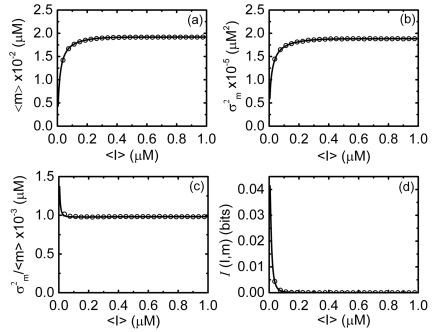
Figure 3: Fluctuations in mRNA. The (a) mean ($\langle m\rangle$), (b) variance ($\sigma^{2}_{m}$), and (c) Fano factor ($\sigma^{2}_{m}/\langle m\rangle$) are plotted with respect to the average signal strength $\langle I\rangle$. In (d) the transmission of information (${\cal I}(I,m)$) in the autoregulation mediated transcription is shown. The symbols are generated using stochastic simulation algorithm Gillespie (1976, 1977) and the lines are due to theoretical expressions.

III.2 Transcriptional randomness

The central dogma of the molecular biology involves two steps - gene transcription, to produce mRNA and further in turn translation, to protein. In the present work, we are interested in the zeroth-order $R_{P}$-regulated transcription from the operon of $R$ and $S$. The accumulation of the mRNA pool is regulated by the first-order degradation of mRNA. $R_{P}$, activated from the phosphotransfer module, binds at the promoter in the form of a feedback with Hill function kinetics, $f(R_{P})=R^{H}_{P}/(K^{H}+R^{H}_{P})$. Here, $K$ (= $20$ $\mu$M) is the equilibrium dissociation constant of the transcription factor $R_{P}$ to the promoter. The Hill coefficient $H=1$, as considered in the current model, corresponds to a positive feedback without any cooperativity. To monitor the stochasticity introduced in the transcriptional kinetics, we quantitate the fluctuations in the pool of the mRNA. Fig. 3(a-c) shows the statistical properties of mRNA expression in response to the signal. For a wide range of signal the variance of mRNA, $\sigma^{2}_{m}$ remains constant and is equal to the average, $\langle m\rangle$ which makes Fano factor equals to unity, a signature of Poissonian statistics. We note that the equality relation between the variance and the mean value can be checked when both the quantities are expressed in copy numbers/cellular volume instead of concentration using the relation 1M $\approx 1.024\times 10^{9}$ copy number/cellular volume. The overall statistical features observed in the mRNA dynamics suggests that the feedback controlled autoregulation and subsequent transcription behave like a fluctuational buffer in the whole network. As a result, a weak information transmission occurs through the autoregulation module (Fig. 3(d)).

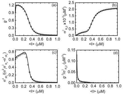
Figure 4: The signaling performance of the TCS. The (a) network gain ($g^{2}$), (b) intrinsic noise ($\sigma^{2}_{R_{P}|I}$), (c) signal-to-noise ratio, and (d) gain-to-noise ratio are presented for the full range of the signal $\langle I\rangle$ at steady state. The symbols are generated using stochastic simulation algorithm Gillespie (1976, 1977) and the lines are due to theoretical expressions.

III.3 The TCS signaling network

In this subsection, we discuss the motivation for considering the TCS motif as a signal transducer. To this end, it is crucial to quantify both the gain and the noise, not in isolation of them. To elucidate the network performance, we consider four different measures: network gain ($g^{2}$), intrinsic noise ($\sigma^{2}_{R_{P}|I}$), signal-to-noise ratio (SNR), and gain-to-noise ratio (GNR). The quantitative measures can be defined Tostevin and ten Wolde (2010) as follows, as the TCS cascade satisfies the spectral addition rule Warren et al. (2006),

$$g^{2} = \frac{\sigma^{2}_{R_{P}I}}{\sigma^{2}_{I}},$$ (13)

$$\sigma^{2}_{R_{P}|I} = \sigma^{2}_{R_{P}}-g^{2}\sigma^{2}_{I},$$ (14)

$$SNR = \frac{\sigma^{4}_{IR_{P}}}{\sigma_{I}^{2}\sigma_{R_{P}}^{2}-\sigma_{IR_{P}}^{4}}=\frac{g^{2}}{\sigma^{2}_{R_{P}|I}}\sigma^{2}_{I},$$ (15)

$$GNR = \frac{g^{2}}{\sigma^{2}_{R_{P}|I}}.$$ (16)

The gain, defined here, is different from the macroscopic gain Savageau (1976); Goldbeter and Koshland (1981); Koshland et al. (1982) which characterises the fold increment in the observable output for a constant signal. The stochastic network gain is a qualitative measure about the uncertainty estimation of the network input when the uncertainty in the output is well known. The GNR gives a better insight on this quantity. It is important to note that the mutual information has an estimation from the reciprocal of the GNR. In Fig. 4(a) the network gain for the current model is being illustrated with respect to the level of the inducer. At low signal strength, the phosphotransfer reactions show determining role in the network, where the fluctuations level of both $R$ and $R_{P}$ grow. Such growth implies the association of the randomness between inducer $I$ and both $R_{P}$ and $R$ increases. This association assists the elevation in the gain value. As the signal increases, the pool of the response regulator gets fully phosphorylated, and the fluctuations strength in the $R_{T}$ pool becomes constant. As a result, the gain and the GNR deplete (Fig. 4(a),4(d)).

The intrinsic noise, explains the randomness within the system, usually occurs through the inherently probabilistic biochemical reactions. Following the spectral addition rule fluctuations due to inducer ($\delta I$) has been eliminated from the fluctuations of the network output ($\delta R_{P}$) to purify the intrinsic noise of the TCS cascade (Eq. (14)). Fig. 4(b) shows the intrinsic noise profile as a function of inducer level. The intrinsic noise is nearly equal to $\sigma^{2}_{R_{P}}$ (shown in Fig. 2(b)) as the contribution of $g^{2}$ is minuscule for increasing signal strength.

The SNR is a good measure of the fidelity for a signaling network. Better the SNR, the better is the reliability of the cascade. The mutual information is the quotient of reliability, and it depends on the SNR. In Fig. 4(c), we show the characteristic profile of SNR vs. inducer. The notion of this plot is to decrypt the effective signal transmission through the signaling channel. The SNR initially starts from a moderate value at a very low signal strength and maximises where the $R_{P}$ population reaches the maximum value. As a consequence of the sharp rise of the fluctuations in $R_{P}$ as well as the intrinsic noise, the SNR experiences a quick decay. From the inclination of fidelity, it is to infer that the TCS shows maximum reliability at low to moderate level of the signal $\langle I\rangle$ when the $R$ to $R_{P}$ transition rate is high.

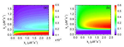
Figure 5: (color online) The role of kinase and phosphatse rate. The two dimensional map of (a) the Fano factor ($\sigma^{2}_{R_{P}}/\langle R_{P}\rangle$) and (b) the mutual information (${\cal I}(I,R_{P})$) as a function of the kinase and phosphatase rate constants of the phosphotransfer module. The maps are drawn using $\langle I\rangle=$ 0.15 $\mu$M. All the other rate parameters are according to Table I.

III.4 Information transmission

The functionality of a two-component system is to sense and respond appropriately to any extracellular signal. As we are considering the associated fluctuations in the signaling pathway, the quantitative reliability in terms of mutual information is to be measured. For a Gaussian system, the mutual information provides the channel capacity Shannon (1948); Cover and Thomas (1991). Considering the inducer ($I$) as network input and phosphorylated response regulator ($R_{P}$) as the output, one can quantify the mutual information ${\cal I}(I,R_{P})$ between $I$ and $R_{P}$. The interplay between the signal and the network response can be verified when the association of the input-output fluctuations space is determined. According to the definition of Shannon Shannon (1948), for Gaussian noise processes, the mutual information can be written as

$${\cal I}(I,R_{P})=\frac{1}{2}\log_{2}\left(1+\frac{\sigma^{4}_{IR_{P}}}{\sigma_{I}^{2}\sigma_{R_{P}}^{2}-\sigma_{IR_{P}}^{4}}\right),$$ (17)

where the quantity $\sigma^{4}_{IR_{P}}/(\sigma_{I}^{2}\sigma_{R_{P}}^{2}-\sigma_{IR_{P}}^{4})$ measures the fidelity (SNR). In Fig. 2(d), we show mutual information as a function of the inducer level. The information processing by the TCS shows a sharp growth followed by a decaying nature. Beyond a certain inducer level, the mutual information profile goes down implying attainment of the steady state of the response regulator pool.

Since the phosphotransfer module plays the dominant role in the TCS cascade, the investigation for the two critical reactions: kinase and phosphatase within the frame of mutual information is crucial. In Fig. 5, we show the contour map of Fano factor and mutual information as a function of the phosphotransfer rate parameters: kinase, $k_{k}$ and phosphatase, $k_{p}$. While the Fano factor of $R_{P}$ measures the output fluctuations at the molecular level, ${\cal I}(I,R_{P})$ quantitates the association between the input and output fluctuations level. So a comparative optimisation of the rate constants is executed here in the two maps. In Fig. 5(a), one can see that at very low phosphatase rate the fluctuations level in $R_{P}$ is maximum; else it is quite low. In the same regime, the information processing is very weak (Fig. 5(b)). The information processing maximises at a moderate phosphatase and high kinase level where the fluctuations level is remarkably low. This happens due to the low amount of $R_{P}$ at high phosphatase activity of the sensor protein, $S$.

For the autoregulated transcription module, the mutual information of the noisy gene expression can be written as

$${\cal I}(I,m)=\frac{1}{2}\log_{2}\left(1+\frac{\sigma^{4}_{Im}}{\sigma_{I}^{2}\sigma_{m}^{2}-\sigma_{Im}^{4}}\right).$$ (18)

The fluctuations space associated with mRNA shown in the profiles of variance and Fano factor (see Figs. 3(b,c)) is so narrow that the intersection of that with the fluctuations space of the inducer is minuscule. It gets also reflected in the profile of the mutual information ${\cal I}(I,m)$ in Fig. 3(d). With the enhancement of the signal strength, the information flow through the transcription reaction attenuates sharply. Since the gene regulation and the transcription in this network play the role of a noise buffer, the sharp decrease in the information processing capacity is well justified.

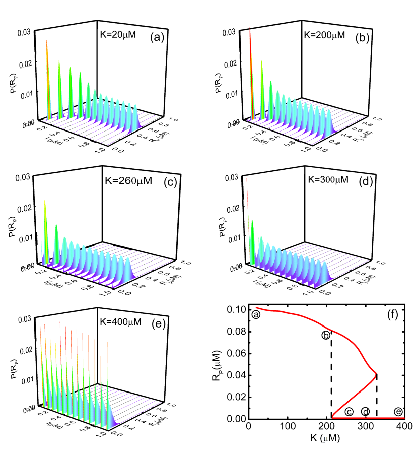
Figure 6: (color online) Noise induced bimodality. (a)-(e) The three dimensional histogram of the probability density of $R_{P}$ at steady state is plotted for different values of the dissociation constant $K$. The $x$-axis shows the level of signal, $I$ and the population of $R_{P}$ is given in the $y$-axis. (f) The mean population of $R_{P}$ with respect to the dissociation constant $K$ at low value of signal ($I=0.075$ $\mu$M). The region inside the dotted lines shows bimodality.

III.5 Protein distribution and the stability switch

In this section, we propose a numerical framework which explores the distribution of the phosphorylated response regulator protein at the steady state. The analysis of the two-component system ascribed above is within the purview of linear noise approximation. Now, we want to extend the same network beyond the linear limit and examine some key features from the distribution profile. Here, we observe the noise propagation through the autoregulation module under the control of the dissociation constant $K$ of the transcription factor $R_{P}$ at the promoter site, as different ranges of $K$ shows different probability distributions for a particular signal strength (Fig. 6(a-e)).

As the dissociation constant $K$ is the ratio of the two rate constants: The unbinding ($k_{u}$) and the binding ($k_{b}$) rate of the transcription factor, the variation in $K$ drives the full regulated expression through the alteration in the promoter kinetics. At lower $K$-value, binding of $R_{P}$ to the promoter is more stable, and the duration of the ‘ON’ state of the promoter is much larger than the ‘OFF’ state. Hence, the transcription reaction incorporates lesser fluctuations in further proceedings. With the increment of $K$ the time scales of the ‘ON’ and the ‘OFF’ state of the promoter appears to be comparable. As a result, two separate regime appears in the transcription timing, and this intrinsic stochasticity introduces distinct bimodality in the population of $R_{P}$. The presence of the weak nonlinearity in $f(R_{P})=R_{P}/(K+R_{P})$ for positive feedback shows a zero-order ultrasensitivity, which always produces single-valued steady-state concentration, i.e. monostability, when characterised deterministically without noise. But the numerical simulation of the stochastic model explores the stability switch which produces multi-valued steady state, i.e., bimodality. In Fig. 6(f), one can see that the bimodal population of $R_{P}$ exists within a very narrow range of $K$. At the exterior of this range, the distribution is unimodal at the low or the high population. If we denote the small copy number state as the persisters, that frequently occurs in a bacterial population, the sharp switch between the two states must have an evolutionary and survival fate.

IV Conclusions

The present study reports a theoretical analysis of signal transduction in bacterial two-component signalling pathway using a stochastic framework. The theoretical study makes a detailed discussion of the fluctuations propagation in the presence of an external signal. We find that the switching of the response regulator in its two states cannot produce more randomness in the protein pool but the observed fluctuations appear to be conveyed through the cascade. The observed Poissonian feature in mRNA pool predicts the transcription system with weak bursts and less noise generation. Our analysis also checks the reliability of the network in information processing. To this end, the fidelity of the network is examined through the signal-to-noise ratio. Our results suggest that the complete network has high efficiency at moderately low level of the signal. In this context, the modular structure of the network is being analysed. The phosphotransfer module takes the leading role in the propagation of fluctuations and information compared to the autoregulation module. The traditional metrics like variance and Fano factor measures the noise strength in the network but is unable to guess how fluctuations affect the process of information transmission. To take care of this issue, we focus on the signalling fidelity. Given the network gain and the intrinsic noise as two antagonistic metrics, an efficient network always tries to maximise the gain at the minimal inherent randomness. A multi-objective trade-off between these two different parameters makes a network more robust against the external stimulus.

The recent advent of experimental techniques facilitates the measure of cellular and molecular fluctuations along with the information flow. The TCS, a minimal example of the bacterial communication system, harvests reliable information transmission while making a cellular decision. The regulation of gene expression is the most crucial physiological function to be decided. But in the case of complex interconnected genetic networks, it is hard to decipher the exact path of noise incorporation or information flow. The modular approach to systems biology at single cell level may help in addressing this issue. The investigation of single-cell behaviour may also reveal the noise-driven bifurcation of a monoclonal population and the existence of a sharp switch between the phenotypes. This switching mechanism may evolve to adapt in an adverse environment. Rather than an evolutionary pressure, the noise makes the regulated gene expression develop towards an optimal state.

Data Availability

All relevant data are within the paper.

Competing Interest

We have no competing interests.

Author Contributions

TM SC SKB conceived and designed the study, TM carried out the theoretical calculation and numerical simulation, TM SKB analyzed the data, TM SC SKB wrote the paper. All authors gave final approval for publication.

*

Appendix A

The fluctuations matrix $\delta\mathbf{X}$, the noise matrix $\mathbf{\Xi}$ and the Jacobian matrix $\mathbf{J}$ written in Eq. (7) are defined as,

$$\delta\mathbf{X}=\left(\begin{array}[]{c}\delta I\\ \delta S_{P}\\ \delta R_{P}\\ \delta m\\ \delta S_{T}\\ \delta R_{T}\end{array}\right),\mathbf{\Xi}=\left(\begin{array}[]{c}\xi_{I}\\ \xi_{S_{P}}\\ \xi_{R_{P}}\\ \xi_{m}\\ \xi_{S_{T}}\\ \xi_{R_{T}}\end{array}\right),$$

$$\mathbf{J}=\left(\begin{array}[]{cccccc}J_{II}&J_{IS_{P}}&J_{IR_{P}}&J_{Im}&J_{IS_{T}}&J_{IR_{T}}\\ J_{S_{P}I}&J_{S_{P}S_{P}}&J_{S_{P}R_{P}}&J_{S_{P}m}&J_{S_{P}S_{T}}&J_{S_{P}R_{T}}\\ J_{R_{P}I}&J_{R_{P}S_{P}}&J_{R_{P}R_{P}}&J_{R_{P}m}&J_{R_{P}S_{T}}&J_{R_{P}R_{T}}\\ J_{mI}&J_{mS_{P}}&J_{mR_{P}}&J_{mm}&J_{mS_{T}}&J_{mR_{T}}\\ J_{S_{T}I}&J_{S_{T}S_{P}}&J_{S_{T}R_{P}}&J_{S_{T}m}&J_{S_{T}S_{T}}&J_{S_{T}R_{T}}\\ J_{R_{T}I}&J_{R_{T}S_{P}}&J_{R_{T}R_{P}}&J_{R_{T}m}&J_{R_{T}S_{T}}&J_{R_{T}R_{T}}\end{array}\right)$$

with

$$J_{II}=-k_{dI},J_{IS_{P}}=J_{IR_{P}}=J_{Im}=J_{IS_{T}}=J_{IR_{T}}=0,$$

$$J_{S_{P}I}=k_{ap}(\langle S_{T}\rangle-\langle S_{P}\rangle),$$

$$J_{S_{P}S_{P}}=-k_{ap}\langle I\rangle-k_{adp}-k_{k}(\langle R_{T}\rangle-\langle R_{P}\rangle)-k_{dp},$$

$$J_{S_{P}R_{P}}=k_{k}\langle S_{P}\rangle,J_{S_{P}m}=0,J_{S_{P}S_{T}}=k_{ap}\langle I\rangle,$$

$$J_{S_{P}R_{T}}=-k_{k}\langle S_{P}\rangle,J_{R_{P}I}=0,$$

$$J_{R_{P}S_{P}}=k_{k}(\langle R_{T}\rangle-\langle R_{P}\rangle)+k_{p}\langle R_{P}\rangle,$$

$$J_{R_{P}R_{P}}=-k_{k}\langle S_{P}\rangle-k_{4}(\langle S_{T}\rangle-\langle S_{P}\rangle)-k_{dp},J_{R_{P}m}=0,$$

$$J_{R_{P}S_{T}}=-k_{p}\langle R_{P}\rangle,J_{R_{P}R_{T}}=k_{k}\langle S_{P}\rangle,J_{mI}=0,J_{mS_{P}}=0,$$

$$J_{mR_{P}}=k_{sm}\left[\frac{\delta f(R_{P})}{\delta R_{P}}\right]_{s.s}=k_{sm}\frac{K}{(\langle R_{P}\rangle+K)^{2}},$$

$$J_{mS_{T}}=J_{mR_{T}}=J_{S_{T}I}=J_{S_{T}S_{P}}=J_{S_{T}R_{P}}=0,$$

$$J_{S_{T}m}=k_{ss},J_{S_{T}S_{T}}=-k_{dp},J_{mm}=-k_{dm},$$

$$J_{S_{T}R_{T}}=J_{R_{T}I}=J_{R_{T}S_{P}}=J_{R_{T}R_{P}}=0,$$

$$J_{R_{T}m}=k_{sr},J_{R_{T}S_{T}}=0,J_{R_{T}R_{T}}=k_{dp}.$$

The explicit form of the diffusion matrix written in Eq. (8) is

$${\bf D}=\left(\begin{array}[]{cccccc}D_{II}&D_{IS_{P}}&D_{IR_{P}}&D_{Im}&D_{IS_{T}}&D_{IR_{T}}\\ D_{S_{P}I}&D_{S_{P}S_{P}}&D_{S_{P}R_{P}}&D_{S_{P}m}&D_{S_{P}S_{T}}&D_{S_{P}R_{T}}\\ D_{R_{P}I}&D_{R_{P}S_{P}}&D_{R_{P}R_{P}}&D_{R_{P}m}&D_{R_{P}S_{T}}&D_{R_{P}R_{T}}\\ D_{mI}&D_{mS_{P}}&D_{mR_{P}}&D_{mm}&D_{mS_{T}}&D_{mR_{T}}\\ D_{S_{T}I}&D_{S_{T}S_{P}}&D_{S_{T}R_{P}}&D_{S_{T}m}&D_{S_{T}S_{T}}&D_{S_{T}R_{T}}\\ D_{R_{T}I}&D_{R_{T}S_{P}}&D_{R_{T}R_{P}}&D_{R_{T}m}&D_{R_{T}S_{T}}&D_{R_{T}R_{T}}\end{array}\right)$$

with

$$D_{II}=2k_{dI}\langle I\rangle,D_{IS_{P}}=D_{IR_{P}}=D_{Im}=D_{IS_{T}}=0,$$

$$D_{IR_{T}}=D_{S_{P}I}=0,D_{S_{P}S_{P}}=2k_{ap}(\langle S_{T}\rangle-\langle S_{P}\rangle)\langle I\rangle,$$

$$D_{S_{P}R_{P}}=-k_{k}\langle S_{P}\rangle(\langle R_{T}\rangle-\langle R_{P}\rangle),D_{S_{p}m}=D_{S_{P}S_{T}}=0,$$

$$D_{S_{P}R_{T}}=D_{R_{P}I}=0,D_{R_{P}S_{P}}=-k_{k}\langle S_{P}\rangle(\langle R_{T}\rangle-\langle R_{P}\rangle),$$

$$D_{R_{P}R_{P}}=2k_{k}\langle S_{P}\rangle(\langle R_{T}\rangle-\langle R_{P}\rangle),D_{R_{P}m}=D_{R_{P}S_{T}}=0,$$

$$D_{R_{P}R_{T}}=D_{mI}=D_{mS_{P}}=D_{mR_{P}}=0,D_{mm}=2k_{dm}\langle m\rangle,$$

$$D_{mS_{T}}=D_{mR_{T}}=D_{S_{T}I}=D_{S_{T}S_{P}}=D_{S_{T}R_{P}}=D_{S_{T}m}=0,$$

$$D_{S_{T}S_{T}}=2k_{dp}\langle S_{T}\rangle,D_{S_{T}R_{T}}=D_{R_{T}I}=D_{R_{T}S_{P}}=0,$$

$$D_{R_{T}R_{P}}=D_{R_{T}m}=D_{R_{T}S_{T}}=0,D_{R_{T}R_{T}}=2k_{dp}\langle R_{T}\rangle.$$

Table 1: List of kinetics schemes and the values of rate parameters used in the model. $f(R_{P})$= $R_{P}/(R_{P}+K)$, with $K=20$ $\mu$M.

Reaction	Kinetics	Propensity	Rate constant
Synthesis of $I$	$\phi\rightarrow I$	$k_{sI}$	$k_{sI}=0.003\ \mu$Ms-1
Degradation of $I$	$I\rightarrow\phi$	$k_{dI}I$	$k_{dI}=0.01\$s-1
Autophosphorylation of $S$	$S+I\rightarrow S_{P}$	$k_{ap}SI$	$k_{ap}=1.0\ \mu$M-1s-1
Autodephosphorylation of $S_{P}$	$S_{P}\rightarrow S$	$k_{adp}S_{P}$	$k_{adp}=0.01$ s-1
Phophotransfer from $S_{P}$ to $R$	$S_{P}+R\rightarrow S+R_{P}$	$k_{k}S_{P}R$	$k_{k}=1.0\ \mu$M-1s-1
Dephosphorylation of $R_{P}$ by $S$	$R_{P}+S\rightarrow R+S$	$k_{p}R_{P}S$	$k_{p}=0.7\ \mu$M-1s-1
$R_{P}$ mediated transcription	$\phi\stackrel{{\scriptstyle f(R_{P})}}{{\longrightarrow}}m$	$k_{sm}f(R_{P})$	$k_{sm}=0.0002\ \mu$Ms-1
Degradation of mRNA	$m\rightarrow\phi$	$k_{dm}m$	$k_{dm}=0.01\$s-1
Translation of $S$ from $m$	$m\rightarrow m+S$	$k_{ss}m$	$k_{ss}=0.02\$s-1
Translation of $R$ from $m$	$m\rightarrow m+R$	$k_{sr}m$	$k_{sr}=0.04\$s-1
Degradation of $S$	$S\rightarrow\phi$	$k_{dp}S$	$k_{dp}=0.0016\$s-1
Degradation of $R$	$R\rightarrow\phi$	$k_{dp}R$	$k_{dp}=0.0016\$s-1
Degradation of $S_{P}$	$S_{P}\rightarrow\phi$	$k_{dp}S_{P}$	$k_{dp}=0.0016\$s-1
Degradation of $R_{P}$	$R_{P}\rightarrow\phi$	$k_{dp}R_{P}$	$k_{dp}=0.0016\$s-1

References

- Balázsi et al. (2011) Balázsi, G., A. van Oudenaarden, and J. J. Collins, 2011, Cell 144, 910.
- Batchelor and Goulian (2003) Batchelor, E., and M. Goulian, 2003, Proc. Natl. Acad. Sci. U.S.A. 100, 691.
- Bishop and Qian (2010) Bishop, L. M., and H. Qian, 2010, Biophys. J. 98, 1.
- Biswas and Banik (2016) Biswas, A., and S. K. Banik, 2016, Phys. Rev. E 93, 052422.
- Cover and Thomas (1991) Cover, T. M., and J. A. Thomas, 1991, Elements of Information Theory (Wiley-Interscience, New York).
- Davidson and Surette (2008) Davidson, C. J., and M. G. Surette, 2008, Annu. Rev. Genet. 42, 253.
- Dubnau and Losick (2006) Dubnau, D., and R. Losick, 2006, Mol. Microbiol. 61, 564.
- Eldar and Elowitz (2010) Eldar, A., and M. B. Elowitz, 2010, Nature 467, 167.
- Elf and Ehrenberg (2003) Elf, J., and M. Ehrenberg, 2003, Genome Res. 13, 2475.
- Friedman et al. (2006) Friedman, N., L. Cai, and X. S. Xie, 2006, Phys. Rev. Lett. 97, 168302.
- Gardiner (2009) Gardiner, C., 2009, Stochastic Methods, 4th ed. (Springer, Berlin).
- Ghosh et al. (2011) Ghosh, S., K. Sureka, B. Ghosh, I. Bose, J. Basu, and M. Kundu, 2011, BMC Syst Biol 5, 18.
- Gillespie (1976) Gillespie, D. T., 1976, J. Comp. Phys. 22, 403.
- Gillespie (1977) Gillespie, D. T., 1977, J. Phys. Chem. 81, 2340.
- Goldbeter and Koshland (1981) Goldbeter, A., and D. E. Koshland, 1981, Proc. Natl. Acad. Sci. U.S.A. 78, 6840.
- Goulian (2010) Goulian, M., 2010, Curr. Opin. Microbiol. 13, 184.
- Grima (2015) Grima, R., 2015, Phys. Rev. E 92, 042124.
- Grima et al. (2011) Grima, R., P. Thomas, and A. V. Straube, 2011, J. Chem. Phys. 135, 084103.
- Groisman (2016) Groisman, E. A., 2016, Annu. Rev. Microbiol. 70, 103.
- Hart and Alon (2013) Hart, Y., and U. Alon, 2013, Mol. Cell 49, 213.
- Hoyle et al. (2012) Hoyle, R. B., D. Avitabile, and A. M. Kierzek, 2012, PLoS Comput. Biol. 8, e1002396.
- Igoshin et al. (2008) Igoshin, O. A., R. Alves, and M. A. Savageau, 2008, Mol. Microbiol. 68, 1196.
- van Kampen (2007) van Kampen, N. G., 2007, Stochastic Processes in Physics and Chemistry, 3rd ed. (North-Holland, Amsterdam).
- Keizer (1987) Keizer, J., 1987, Statistical Thermodynamics of Nonequilibrium Processes (Springer-Verlag, Berlin).
- Kierzek et al. (2010) Kierzek, A. M., L. Zhou, and B. L. Wanner, 2010, Mol Biosyst 6, 531.
- Koshland et al. (1982) Koshland, D. E., A. Goldbeter, and J. B. Stock, 1982, Science 217, 220.
- Laub and Goulian (2007) Laub, M. T., and M. Goulian, 2007, Annu. Rev. Genet. 41, 121.
- Maity et al. (2014) Maity, A. K., A. Bandyopadhyay, P. Chaudhury, and S. K. Banik, 2014, Phys. Rev. E 89, 032713.
- Maity et al. (2015) Maity, A. K., P. Chaudhury, and S. K. Banik, 2015, PLoS ONE 10, e0123242.
- Mehta et al. (2008) Mehta, P., S. Goyal, and N. S. Wingreen, 2008, Mol. Syst. Biol. 4, 221.
- Micali and Endres (2016) Micali, G., and R. G. Endres, 2016, Curr. Opin. Microbiol. 30, 8.
- Ortega et al. (2002) Ortega, F., L. Acerenza, H. V. Westerhoff, F. Mas, and M. Cascante, 2002, Proc. Natl. Acad. Sci. U.S.A. 99, 1170.
- Paulsson (2004) Paulsson, J., 2004, Nature 427, 415.
- Paulsson (2005) Paulsson, J., 2005, Phys Life Rev 2, 157.
- Raj and van Oudenaarden (2008) Raj, A., and A. van Oudenaarden, 2008, Cell 135, 216.
- Sanchez and Kondev (2008) Sanchez, A., and J. Kondev, 2008, Proc. Natl. Acad. Sci. U.S.A. 105, 5081.
- Savageau (1976) Savageau, M. A., 1976, Biochemical Systems Analysis: A Study of Function and Design in Molecular Biology (Addison-Wesley, Readling, Massachusetts).
- Shannon (1948) Shannon, C. E., 1948, Bell. Syst. Tech. J 27, 379.
- Shinar et al. (2007) Shinar, G., R. Milo, M. R. Martinez, and U. Alon, 2007, Proc. Natl. Acad. Sci. U.S.A. 104, 19931.
- Spiller et al. (2010) Spiller, D. G., C. D. Wood, D. A. Rand, and M. R. White, 2010, Nature 465, 736.
- Stock et al. (2000) Stock, A. M., V. L. Robinson, and P. N. Goudreau, 2000, Annu. Rev. Biochem. 69, 183.
- Swain (2004) Swain, P. S., 2004, J. Mol. Biol. 344, 965.
- Tǎnase-Nicola et al. (2006) Tǎnase-Nicola, S., P. B. Warren, and P. R. ten Wolde, 2006, Phys. Rev. Lett. 97, 068102.
- Tiwari et al. (2010) Tiwari, A., G. Balázsi, M. L. Gennaro, and O. A. Igoshin, 2010, Phys. Biol. 7, 036005.
- Tiwari et al. (2011) Tiwari, A., J. C. Ray, J. Narula, and O. A. Igoshin, 2011, Math. Biosci. 231, 76.
- Tostevin and ten Wolde (2010) Tostevin, F., and P. R. ten Wolde, 2010, Phys. Rev. E 81, 061917.
- Tsimring (2014) Tsimring, L. S., 2014, Rep Prog Phys 77, 026601.
- Warren et al. (2006) Warren, P. B., S. Tǎnase-Nicola, and P. R. ten Wolde, 2006, J. Chem. Phys. 125, 144904.
- Wei et al. (2014) Wei, K., M. Moinat, T. R. Maarleveld, and F. J. Bruggeman, 2014, Mol. Biosyst. 10, 2338.
- Yang et al. (2015) Yang, X., Y. Wu, and Z. Yuan, 2015, Int. J Bifurcation and Chaos 25, 1540010.