A New Class of High-Order Methods for Fluid Dynamics Simulations using Gaussian Process Modeling

Abstract

We introduce an entirely new class of high-order methods for computational fluid dynamics (CFD) based on the Gaussian Process (GP) family of stochastic functions. Our approach is to use kernel-based GP prediction methods to interpolate/reconstruct high-order approximations for solving hyperbolic PDEs. We present the GP approach as a new formulation of high-order (magneto)hydrodynamic state variable interpolation that furnishes an alternative to conventional polynomial-based approaches.

1 Introduction

Cutting edge simulations of gas dynamics and magnetohydrodynamics (MHD) have been among the headliner applications of scientific high-performance computing (HPC) Dongarra2012future ; Dongarra2010recent ; Keyes2013multiphysics ; Subcommittee2014top . They are expected to remain important as new HPC architectures of ever more powerful capabilities come online in the decades to come. A notable trend in recent HPC developments concerns the hardware design of the newer architectures: It is expected that newer HPC architectures will feature a radical change in the balance between computation and memory resources, with memory per compute core declining dramatically from current levels Attig2011 ; Dongarra2012future ; Subcommittee2014top . This trend tells us that new algorithmic strategies will be required to meet the goals of saving memory and accommodating increased computation. This paradigm shift in designing scientific algorithms has become a great import in HPC applications. In the context of numerical methods for computational fluid dynamics (CFD), one desirable approach is to design high-order accurate methods Subcommittee2014top that, in contrast to low-order methods, can achieve an increased target solution accuracy more efficiently and quickly by computing increased higher-order floating-point approximations on a given grid resolution Hesthaven2007 ; LeVeque2002 ; leveque2007finite . This approach embodies in a concrete manner the desired tradeoff between memory and computation by exercising more computation per memory – or equivalently, the equal amount of computation with less memory.

Within the broad framework of finite difference method (FDM) and finite volume method (FVM) discretizations, discrete algorithms of data interpolation and reconstruction play a key role in numerical methods for PDE integration LeVeque2002 ; leveque2007finite ; toro2009 . They are frequently the limiting factor in the convergence rate, efficiency, and algorithmic complexity of a numerical scheme. The general procedure in 1D high-order conservative FDM is to pursue high-order approximations of flux function values ${\hat{F}_{i+\frac{1}{2}}}$ at interfaces, by interpolating the set of the interface flux function values $\{F(q_{i-p}),\dots,F(q_{i+r})\}$, each of which is evaluated as pointwise value at $q_{k},k=i-p,\dots,i+r$, for some integers $p$ and $r$. Mathematically, this is formulated as

$$\hat{F}_{i+\frac{1}{2}}=\mathcal{I}\Big{(}F(q_{i-p}),\dots,F(q_{i+r})\Big{)},$$ (1)

where $\mathcal{I}(\cdot)$ is a highly accurate interpolation scheme providing stable numerical interface flux values that are evaluated as pointwise values of $q_{k}$ over a stencil of interpolation, $\cup_{k=i-p}^{i+r}I_{k}$, where $I_{k}$ denotes the $k$-th cell (e.g., $[x_{i-1/2},x_{i+1/2}]$ in 1D) jiang1996efficient ; Mignone2010b . By contrast, the procedure of 1D high-order FVM begins with a set of the cell volume-averaged values

$$\langle q_{i}\rangle=\frac{1}{\Delta x}\int_{\Delta x}q(x,t^{n})dx$$ (2)

as initial conditions, and seeks a pair of high-order accurate reconstructed pointwise Riemann state values

$$({q}_{i+\frac{1}{2}}^{L},{q}_{i+\frac{1}{2}}^{R})=\mathcal{R}\Big{(}\langle q_{i-p}\rangle,\dots,\langle q_{i+r}\rangle\Big{)}$$ (3)

at the cell interfaces $x_{i+\frac{1}{2}}$ using a high-order reconstruction scheme $\mathcal{R}(\cdot)$ over the stencil of reconstruction, $\cup_{k=i-p}^{i+r}I_{k}$. High-order FV fluxes ${\hat{F}_{i+\frac{1}{2}}}$ are then evaluated by solving Riemann problems at the interfaces $x_{i+\frac{1}{2}}$ using the Riemann state pair $({q}_{i+\frac{1}{2}}^{L},{q}_{i+\frac{1}{2}}^{R})$ as inputs buchmuller2014improved ; lee2013solution ; LeVeque2002 ; mccorquodale2011high ; shu2009high ; toro2009 .

More generally, interpolation and reconstruction are not only essential for estimating high-order accurate approximations for fluxes at quadrature points on each cell, but also for interface tracking; for prolonging states from coarse zones to corresponding refined zones in adaptive-mesh refinement (AMR) schemes; and for various other contexts associated with high-order solutions. In CFD simulations, these interpolation and reconstruction algorithms must be carried out as accurately as possible, because, to a large extent, their accuracy is one of the key factors that determines the overall accuracy of the simulation.

Polynomial-based approaches are the most successful and popular among interpolation/reconstruction methods in this field. There are a couple of convincing reasons for this state of affairs. First, they are easily relatable to Taylor expansion, the most familiar of function approximations. Second, the nominal $N$-th order accuracy of polynomial interpolation/reconstruction is derived from using polynomials of degree $(N-1)$, bearing a leading term of the error that scales with $\mathcal{O}(\Delta^{N})$ as the local grid spacing $\Delta$ approaches to zero LeVeque2002 ; leveque2007finite ; toro2009 . However, the simplicity of polynomial interpolation/reconstruction comes at a price: The polynomial approach is notoriously prone to oscillations in data fitting, especially with discontinuous data Gottlieb1997 ; Furthermore, in many practical situations the high-order polynomial interpolation/reconstruction must be carried out on a fixed size of stencils, whereby there is a one-to-one relationship between the order of the interpolation/reconstruction and the size of the stencils. This becomes a restriction in particular when unstructured meshes are considered in multiple spatial dimensions. Lastly, another related major issue lies in the fact that the algorithmic complexity of such polynomial based schemes typically grows with order of accuracy Gerolymos2009 , as well as with spatial dimensionality buchmuller2014improved ; mccorquodale2011high ; zhang2011order in FVM.

To overcome the aforementioned issues in polynomial methods, practitioners have developed in the last decades the so-called “non-polynomial” interpolation/reconstruction based on the mesh-free Radial Basis Function (RBF) approximations. The core idea is to replace the polynomial interpolants with RBFs, which is a part of a very general class of approximants from the field known as Optimal Recovery (OR) wendland2010 . Several interpolation techniques in OR have shown practicable in the framework of solving hyperbolic PDEs Katz2009 ; morton2007 ; sonar1996 , parabolic PDEs moroney2006 ; moroney2007 , diffusion and reaction-diffusion PDEs shankar2015radial , boundary value problems of elliptic PDEs liu2015kansa , interpolations on irregular domains chen2016reduced ; heryudono2010radial ; martel2016stability , and also interpolations on a more general set of scattered data Franke1982 . Historically, RBFs were introduced to seek exact function interpolations powell1985radial . Recently, the RBF approximations have been combined with the key ideas of handling discontinuities in the ENO harten1987uniformly and WENO jiang1996efficient ; liu1994weighted methods. Such approaches, termed as ENO/WENO-RBF, have been extended to solve nonlinear scalar equations and the Euler equations in the FDM jung2010recovery and the FVM guo2017rbf frameworks. These studies focused on designing their RBF methods with the use of adaptive shape parameters to control local errors. Also in bigoni2016adaptive , two types of multiquadrics and polyharmonic spline RBFs were used to model the Euler equations with a strategy of selecting optimal shape parameters for different RBF orders. Stability analysis on the fully discretized hyperbolic PDEs in both space and time using the multiquadrics RBF is reported in chen2012matrix . While there exist a few conceptual resemblances between these RBF approaches and our new GP method, the fundamental differences that distinguish the two approaches are discussed later in this paper.

The goal in this article is to develop a new class of high-order methods that overcomes the aforementioned difficulties in polynomial approaches by exploiting the alternative perspective afforded by GP modeling, a methodology borrowed from the field of statistical data modeling. In view of the novelty of our approach, which bridges the two distinct research fields of statistical modeling and CFD, it is our intention in this paper to first construct a mathematical formulation in 1D framework. The current study will serve as a theoretical foundation for later multidimensional extensions of the GP modeling for CFD applications, topics of which will be studied in our future work.

The GP method is a class of high-order schemes primarily designed for numerical evolution of hyperbolic PDEs, $q_{t}+\nabla\cdot F(q)=0$. To this end, we describe the new high-order Gaussian Process (GP) approximation strategies in two steps:

1. GP interpolation that works on pointwise values of $q(x_{i})$ as both inputs and outputs, and

2. GP reconstruction that works on volume-averaged values $\langle q_{i}\rangle=\frac{1}{\Delta x}\int_{\Delta x}q(x,t^{n})dx$ as inputs, reconstructing pointwise values as outputs.

GP interpolation will provide a “baseline” formulation of using GP as a new high-order interpolator operating on the same data type, while GP reconstruction will serve as a high-order reconstructor operating on two different types of data.

2 Gaussian Process Modeling

The theory of GP, and more generally of stochastic functions, dates back to the work of Wiener wiener1949 and Kolmogorov kolmogorov1941 . Modern-day applications are numerous: Just in the physical sciences, GP prediction is in common use in meteorology, geology, and time-series analysis bishop2007pattern ; rasmussen2005 ; wahba1995 , and in cosmology, where GP models furnish the standard description of the Cosmic Microwave Background bond1999 . Applications abound in many other fields, in particular wherever spatial or time-series data requires “nonparametric” modeling bishop2007pattern ; rasmussen2005 ; stein1999 . Within the perspective of CFD applications, our goal in this study is to use predictive GP modeling that is processed by training observed data, (e.g., cell-averaged fluid variables at cell centers) to produce a “data-informed” prediction (e.g., pointwise Riemann state values at cell interfaces). In what follows we give a brief overview on GP from statistical perspective (Section 2.1), followed by our strategies of tuning GP for high-order interpolation (Section 2.2) and reconstruction (Section 2.3) in CFD applications. Readers who wish to pursue the subject in greater detail are referred to bishop2007pattern ; rasmussen2005 ; stein1999 .

2.1 GP – Statistical Perspective

GP is a class of stochastic processes, i.e., processes that sample functions (rather than points) from an infinite dimensional function space. Initially one specifies a so-called prior probability distribution over the function space. Then, given a sample of function values at some set of points, one “trains” the model by regarding the sample as data and using Bayes’ theorem to update the probability distribution over the function space. This way, one obtains a data-informed posterior probability distribution over the function space, adjusted with respect to the prior so as to be compatible with the observed data. The posterior distribution may be used to predict (probabilistically) the value of the function at points where the function has not yet been sampled. The mean value of this GP prediction is our target interpolation/reconstruction for FDM and FVM.

Formally, a GP is a collection of random variables, any finite collection of which has a joint Gaussian distribution bishop2007pattern ; rasmussen2005 . A GP is fully defined by two functions:

• a mean function $\bar{f}(\mathbf{x})=\mathbb{E}[f(\mathbf{x})]$ over $\mathbb{R}^{N}$, and

• a covariance function which is a symmetric, positive-definite integral kernel $K(\mathbf{x},\mathbf{y})$ over $\mathbb{R}^{N}\times\mathbb{R}^{N}$.

Such functions $f$, drawn randomly from this distribution, are said to be sampled from a Gaussian Process with mean function $\bar{f}(\mathbf{x})$ and covariance function $K(\mathbf{x},\mathbf{y})$, and we write $f\sim\mathcal{GP}(\bar{f},K)$. As with the case of finite-dimensional Gaussian distributions, the significance of the covariance is

$$K(\mathbf{x},\mathbf{y})=\mathbb{E}[\left(f(\mathbf{x})-\bar{f}(\mathbf{x})\right)\left(f(\mathbf{y})-\bar{f}(\mathbf{y})\right)],$$ (4)

where the averaging is over the GP distribution.

In standard statistical modeling practice, both $\bar{f}(\mathbf{x})$ and $K(\mathbf{x},\mathbf{y})$ are typically parametrized functions, with parameters controlling the character (e.g. length scales, differentiability, oscillation strength) of “likely” functions. Given a GP, and given $N$ “training” points $\mathbf{x}_{i}$, $i=1,\ldots,N$ at which the function values $f(\mathbf{x}_{i})$ are known, we may calculate the likelihood $\mathcal{L}$ (the probability of $\mathbf{f}$ given the GP model) of the data vector $\mathbf{f}\equiv[f(\mathbf{x}_{1}),\ldots,f(\mathbf{x}_{N})]^{T}$ (e.g., $N$ many pointwise values of density $\rho$ at $\mathbf{x}_{i}$, $i=1,\ldots,N$) by

$$\mathcal{L}\equiv P(\mathbf{f})=(2\pi)^{-\frac{N}{2}}\det|\mathbf{K}|^{-\frac{1}{2}}\exp\left[-\frac{1}{2}\left(\mathbf{f}-\bar{\mathbf{f}}\right)^{T}\mathbf{K}^{-1}\left(\mathbf{f}-\bar{\mathbf{f}}\right)\right],$$ (5)

where $\mathbf{K}=[{K}_{ij}]_{i,j=1,\dots,N}$ with $K_{ij}\equiv K(\mathbf{x}_{i},\mathbf{x}_{j})$.

Given the function samples $\mathbf{f}=[f(\mathbf{x}_{1}),\ldots,f(\mathbf{x}_{N})]^{T}$ obtained at spatial points $\mathbf{x}_{i}$, $i=1,\ldots,N$, GP predictions aim to make a probabilistic statement about the value $f_{*}\equiv f(\mathbf{x}_{*})$ of the unknown function $f\sim\mathcal{GP}(\bar{f},K)$ at a new spatial point $\mathbf{x}_{*}$. In other words, from a stochastic modeling view point, we are interested in making a new prediction of GP for $f$ at any randomly chosen point $\mathbf{x}_{*}$. This is particularly of interest to us from the perspectives of FDM and FVM, because we can use GP to predict an unknown function value at cell interfaces (e.g., $u_{i\pm\frac{1}{2}}$ in 1D) where both FDM and FVM require estimates of flux functions.

We can accomplish this by utilizing the conditioning property of GP from the theory of Bayesian inference bishop2007pattern ; rasmussen2005 . We look at the augmented likelihood function $\mathcal{L}_{*}$ by considering the joint distribution of the currently available training outputs, $\mathbf{f}$, and the new test output $f_{*}$,

$$\mathcal{L}_{*}\equiv P\left(\mathbf{f},f_{*}\right)=(2\pi)^{-\frac{N+1}{2}}\det|\mathbf{M}|^{-\frac{1}{2}}\exp\left[-\frac{1}{2}\left(\mathbf{g}-\bar{\mathbf{g}}\right)^{T}\mathbf{M}^{-1}\left(\mathbf{g}-\bar{\mathbf{g}}\right)\right],$$ (6)

where $\mathbf{g}$ and $\bar{\mathbf{g}}$ are the $(N+1)$-dimensional vectors whose components, in partitioned form, are

$$\mathbf{g}\equiv\left[f_{*},\mathbf{f}\right]^{T},\;\;\;\bar{\mathbf{g}}\equiv\left[\bar{f}(\mathbf{x}_{*}),\bar{\mathbf{f}}\right]^{T},$$ (7)

and $\mathbf{M}$ is the $(N+1)\times(N+1)$ augmented covariance matrix, given in partitioned form by

$$\mathbf{M}=\left(\begin{array}[]{cc}k_{**}&\mathbf{k}_{*}^{T}\\ \mathbf{k}_{*}&\mathbf{K}\end{array}\right).$$ (8)

In Eq. (8), we’ve defined a scalar $k_{**}$ and an $N$-dimensional vector $\mathbf{k}_{*}=[\mathbf{k}_{*,i}]_{i=1,\dots,N}$ given by

$$k_{**}\equiv K(\mathbf{x}_{*},\mathbf{x}_{*}),\;\;\;\mathbf{k}_{*,i}\equiv K(\mathbf{x}_{*},\mathbf{x}_{i}).$$ (9)

Using Bayes’ Theorem, the conditioning property applied to the joint Gaussian prior distribution on the observation $\mathbf{f}$ yields the Gaussian posterior distribution of $f_{*}$ given $\mathbf{f}$. One may then straightforwardly derive bishop2007pattern ; rasmussen2005 :

$$P(f_{*}|\mathbf{f})=\left(2\pi U^{2}\right)^{-\frac{1}{2}}\exp\left[-\frac{\left(f_{*}-\bar{f_{*}}\right)^{2}}{2U^{2}}\right],$$ (10)

where the newly updated posterior mean function is

$${\tilde{f}_{*}}\equiv\bar{f}(\mathbf{x}_{*})+\mathbf{k}_{*}^{T}\mathbf{K}^{-1}\cdot\left(\mathbf{f}-\bar{\mathbf{f}}\right),$$ (11)

and the newly updated posterior covariance is

$$U^{2}\equiv k_{**}-\mathbf{k}_{*}^{T}\mathbf{K}^{-1}\cdot\mathbf{k}_{*}.$$ (12)

What has happened here is that the GP on the unknown function $f$, trained on the data $\mathbf{f}$, has resulted in a Gaussian posterior probability distribution on the unknown function value ${{f}(\mathbf{x}_{*})}$ at a new desired location $\mathbf{x}_{*}$, with a mean $\tilde{f}_{*}$ as given in Eq. (11), and with a variance as given in Eq.  (12).

It is worthwhile to make an important observation at this point. Eq. (5) provides a clear conceptual difference in interpolations and reconstructions between the GP predictions and the RBF approximations. In the GP nonparametric viewpoint we define a prior (or latent) probability distribution directly over function spaces, hence there is no need to seek any fixed number of parameters that may depend on the datasets under consideration. This way, the stochastic properties of functions in the prior are set by a choice of covariance kernel functions, by which the posterior predictions in Eq. (6) follow.

On the contrary, RBF models in the context of interpolations and reconstructions follow the parametric modeling paradigm, requiring to solve a linear system $\mathbf{A}\boldsymbol{\lambda}=\mathbf{F}$ (see e.g., bigoni2016adaptive ; Katz2009 ) whose size is determined and fixed by the number of desired $N$ interpolation points $\mathbf{f}=[f(\mathbf{x}_{1}),\dots,f(\mathbf{x}_{N})]^{T}$ and the associated coefficients (or parameters) $\lambda_{j}$ and $c_{k}$ of an RBF interpolating function $s(\mathbf{x})$,

$$s(\mathbf{x})=\sum_{j=1}^{N}\lambda_{j}\Phi(||\mathbf{x}-\mathbf{x}_{j}||,\epsilon_{j})+\sum_{k=1}^{K}c_{k}p_{k}(\mathbf{x}).$$ (13)

The components of the solution vector $\boldsymbol{\lambda}$ are $\lambda_{j}$ and $c_{k}$, $\mathbf{A}$ is the matrix whose components are set by the values of RBFs $\Phi_{i,j}=\Phi(||\mathbf{x}_{i}-\mathbf{x}_{j}||,\epsilon_{j})$ at two points $\mathbf{x}_{i}$ and $\mathbf{x}_{j}$ and the shape parameter $\epsilon_{j}>0$, $\mathbf{F}$ is the vector with entries of $\mathbf{f}$, and the last term in Eq. (13) is a polynomial (at most) $K$-th degree with $k$-th standard basis polynomials $p_{k}$. Unlike GP, a probability distribution (if needed) is not directly imposed on $s(\mathbf{x})$, rather, it can only be induced by a prior distribution defined on the coefficients.

Even though the two approaches resemble each other in terms of using “kernels” (i.e., RBFs and covariance kernel functions), they are fundamentally different from these statistical viewpoints.

2.2 High-order GP Interpolation for CFD

In this paper we are most interested in developing a high-order reconstruction method for FVM in which the function samples $\mathbf{f}$ are given as volume-averaged data $\langle u_{i}\rangle$. However, we first consider an interpolation method which uses pointwise data $u_{i}$ as function samples $\mathbf{f}$. An algorithmic design for GP interpolation using pointwise data will provide a good mathematical foundation for FVM which reconstructs pointwise values from volume-averaged data.

The mean ${\tilde{f}_{*}}$ of the distribution given in Eq. (11) is our interpolation of the function $f$ at the point $\mathbf{x}_{*}\in\mathbb{R}^{D}$, $D=1,2,3$, where $f$ is any given fluid variable such as density, pressure, velocity fields, magnetic fields, etc. For the purpose of exposition, let us use $q$ to denote one of such fluid variables (e.g., density $\rho=\rho(\mathbf{x},t^{n})$). Also, the mathematical descriptions of both interpolation and reconstruction will be considered in 1D hereafter.

We are interested in seeking a high-order interpolation of ${q}$ at $\mathbf{x}_{*}=x_{*}=x_{i\pm\frac{1}{2}}$ on a stencil $\cup_{k=i-p}^{i+r}I_{k}$,

$${q}_{i\pm\frac{1}{2}}=\mathcal{I}_{GP}(q_{i-p},\dots,q_{i+r}),$$ (14)

where $\mathcal{I}_{GP}(\cdot)$ is the GP interpolation given in Eq. (11). We define

$$\mathbf{f}=[q_{i-p},\dots,q_{i+r}]^{T}.$$ (15)

Furthermore, if we simply assume a constant mean $f_{0}$ for the data in Eq. (15) we get

$$\bar{\mathbf{f}}=f_{0}\mathbf{1}_{r-p+1},\;\;\;\bar{{f}}(x_{i\pm\frac{1}{2}})=f_{0},$$ (16)

where $\mathbf{1}_{r-p+1}=[1,\dots,1]^{T}$ is an $(r-p+1)$-dimensional one-vector. In case of a zero mean $f_{0}=0$ the GP interpolation scheme simply becomes

$${q}_{i\pm\frac{1}{2}}=\mathbf{k}_{i\pm\frac{1}{2}}^{T}\mathbf{K}^{-1}\cdot\mathbf{f}.$$ (17)

As shown in Eqs. (11) and (17), the interpolant $\tilde{f}_{*}=q_{i\pm\frac{1}{2}}$ is a simple linear combination of the observed data $\mathbf{f}$ and the covariance kernels $\mathbf{k_{*}}$ and $\mathbf{K}$, anchored by one of its arguments to one of the data points, $x_{*},x_{i-p},\dots,x_{i+r}$. The second term in Eq. (11) can also be cast as an inner product between a vector of weights $\mathbf{w}^{T}\equiv\mathbf{k}_{*}^{T}\mathbf{K}^{-1}$ and a vector of data residuals $(\mathbf{f}-\bar{\mathbf{f}})$.

The weights $\mathbf{w}$ are independent of the data values $\mathbf{f}$; they depend only on the locations of the data points ${x}_{i}$ and on the desired interpolation point ${x}_{*}$. This is useful, because in hydrodynamic simulations the training point locations (viz. a GP stencil) and the interpolation points (viz. cell interfaces) are often known in advance, as is the case with static Cartesian grid configurations. In such cases, the weight vector $\mathbf{w}$ can be computed and stored in advance at an initialization step and remain constant throughout the simulation. When an adaptive mesh refinement (AMR) configuration is considered, $\mathbf{w}$ can be computed for all possible grid refinement levels and stored a priori for later use. The GP interpolations then come at the cost of the remaining inexpensive inner product operation between $\mathbf{w}^{T}$ and $(\mathbf{f}-\bar{\mathbf{f}})$ in Eq. (11), whose operation count is linearly proportional to the number of points in the stencil. Typically in 1D, the size of the stencil is one for the first order Godunov (FOG) method godunov1959difference ; toro2009 ; three for 2nd order piecewise linear methods (PLM) toro2009 ; van1979towards ; five for both the 3rd order piecewise parabolic method (PPM) colella1984piecewise ; and 5th order Weighted Essentially Non-oscillatory (WENO) method jiang1996efficient . Given such stencil sizes, the cost of the linear solves required by Eq. (11) are minor. For instance, $\mathbf{K}$ is a $5\times 5$ matrix when using a stencil of five grid points, namely, the 5-point GP stencil centered at $x_{i}$ with a radius of two-cell length $S_{2}=\cup_{k=i-2}^{i+2}I_{k}$. In general, we define a stencil $S_{R}$ centered at $x_{i}$ with a radius $R$ cell-length,

$$S_{R}=\bigcup\limits_{k=i-R}^{i+R}I_{k}.$$ (18)

Note that the interpolation point $x_{*}$ may be anywhere in the continuous interval $S_{R}$.

Since the matrix $\mathbf{K}$ is symmetric positive-definite, the inversion of $\mathbf{K}$ can be obtained efficiently by Cholesky decomposition which is about a factor 2 faster than the usual LU decomposition. The decomposition is only needed once, at initialization time, for the calculation of the vector of weights $\mathbf{w}$.

An important feature of GP interpolation is that it naturally supports multidimensional stencil configurations. The reason for this is that there are many valid covariance functions over $\mathbf{R}^{D}$ that are isotropic, and therefore do not bias interpolations and reconstructions along any special direction. The possibility of directionally-unbiased reconstruction over multidimensional stencils is a qualitative advantage of GP interpolation, especially when designing high-order algorithms buchmuller2014improved ; mccorquodale2011high ; zhang2011order . Such high-order multidimensional GP methods will be studied in our future work.

There is an additional piece of information beyond the point estimate $\tilde{f}_{*}$. We also have an uncertainty in the estimate, given by $U$ in Eq. (12). This posterior uncertainty is of crucial importance in many GP modeling applications, but it is of limited interest for the purpose of this paper. We will overlook posterior uncertainty in the current study, and focus on the posterior mean formula given in Eq. (11).

2.3 High-order GP Reconstruction for CFD

In FVM the fluid variables to be evolved are not pointwise values, but rather are volume-averaged integral quantities, $\langle{q}_{i}\rangle=\frac{1}{\Delta{\cal V}_{i}}\int_{\Delta{\cal V}_{i}}q(\mathbf{x},t^{n})d{\cal V}$. In FDM on the other hand, the main task is to find a high-order approximation to the interface flux values $\hat{F}_{{i+\frac{1}{2}}}$, given the fact that their integral quantities $F(q_{i})=\frac{1}{\Delta x}\int_{x_{i-\frac{1}{2}}}^{x_{i+\frac{1}{2}}}\hat{F}(\xi)d\xi$ are known via the analytic evaluations of the flux function $F$ at the given pointwise data set $u_{i}$. The conservative FDM updates in 1D then readily proceed by solving

$$\frac{dq_{i}}{dt}+\frac{1}{\Delta x}\left(\hat{F}_{i+\frac{1}{2}}-\hat{F}_{i-\frac{1}{2}}\right)=0.$$ (19)

In both cases, we see that there is a change in data types – hence the name “reconstruction” – between input (e.g., $\langle q_{i}\rangle$ for FVM; $F(q_{i})$ for FDM) and output (e.g., $q(\mathbf{x},t^{n})$ for FVM; $\hat{F}_{i+\frac{1}{2}}$ for FDM) pairs in such a way that high-order approximations are applied to the integral quantities (inputs) and produce corresponding pointwise values (outputs), with high accuracy.

The GP interpolation method outlined in Section 2.2 should therefore be modified so that reconstruction may account for such data type changes in both FDM and FVM. Note that the integral averages over a grid cell constitute “linear” operations on a function $f(\mathbf{x})$. As with ordinary finite-dimensional multivariate Gaussian distributions, where linear operations on Gaussian random variables result in new Gaussian random variables with linearly transformed means and covariances, a set of $N$ linear functionals operating on a GP-distributed function $f$ has an $N$-dimensional Gaussian distribution with mean and covariance that are linear functionals of the GP mean function and covariance function.

Suppose for example in a FVM sense, we consider a GP reconstruction on a GP stencil $\cup_{k=i-p}^{i+r}I_{k}$. First we define $r-p+1$ measures $dg_{k}(\mathbf{x})$, $k=i-p,\ldots,i+r$, defining $r-p+1$ linear functionals,

$$G_{k}\equiv\int f(\mathbf{x})\,dg_{k}(\mathbf{x}),\;k=i-p,\ldots,i+r.$$ (20)

For the sake of a reconstruction scheme on a mesh of control volumes, we choose the measures $dg_{k}(\mathbf{x})$ to be the cell volume-average measures,

$$dg_{k}(\mathbf{x})=\begin{cases}\displaystyle d^{3}\mathbf{x}\times\prod_{d=x,y,z}\frac{1}{\Delta^{(d)}}&\mbox{ if }\mathbf{x}\in I_{k},\\ \\ 0&\mbox{ if }\mathbf{x}\notin I_{k},\end{cases}$$ (21)

where $\Delta^{(d)}$ is the grid spacing in the $d$-direction, and the $k$-th cell $I_{k}$ is given by $I_{k}=\prod_{d=x,y,z}I_{k}^{(d)}$ with 1D cells $I_{k}^{(d)}=[x_{k}^{(d)}-\frac{\Delta^{(d)}}{2},x_{k}^{(d)}+\frac{\Delta^{(d)}}{2}]$ for each $d$-direction. For the purpose of the current discussion, we will assume a locally-uniform rectilinear grid of cubical cells $I_{k}$ of uniform size $\Delta=\Delta^{(x)}=\Delta^{(y)}=\Delta^{(z)}$.

Then, the vector $\mathbf{G}=[G_{i-p},\ldots,G_{i+r}]^{T}$ is normally distributed with mean $\bar{\mathbf{G}}=[\bar{G}_{i-p},\ldots,\bar{G}_{i+r}]^{T}$ and covariance matrix $\mathbf{C}=\left[\mathbf{C}_{kh}\right]_{k,h=i-p,\dots,i+r}$, where

$$\bar{G}_{k}=\mathbb{E}[G_{k}]=\int\mathbb{E}[f(\mathbf{x})]\,dg_{k}(\mathbf{x})=\int\bar{f}(\mathbf{x})\,dg_{k}(\mathbf{x}),$$ (22)

and

$$\mathbf{C}_{kh} = \mathbb{E}[\left(G_{k}-\bar{G}_{k}\right)\left(G_{h}-\bar{G}_{h}\right)]$$ (23)

$$= \int\mathbb{E}[\left(f(\mathbf{x})-\bar{f}(\mathbf{x})\right)\left(f(\mathbf{y})-\bar{f}(\mathbf{y})\right)]\,dg_{k}(\mathbf{x})\,dg_{h}(\mathbf{y})$$

$$= \int K(\mathbf{x},\mathbf{y})\,dg_{k}(\mathbf{x})\,dg_{h}(\mathbf{y}).$$

Thus, we see that the GP distribution on the function $f$ leads to a multivariate Gaussian distribution on any $(r-p+1)$-dimensional vector $\mathbf{G}$ of linear functionals of $f$. This Gaussian distribution can be used for likelihood maximization in a manner completely analogous to the case of interpolation, where training is performed using pointwise data.

For reconstruction, it is also not hard to generalize Eq. (11). We first define the $(r-p+1)$-dimensional prediction vector $\mathbf{T}_{*}=\left[\mathbf{T}_{*,k}\right]_{k=i-p,\dots,i+r}$ at $\mathbf{x}_{*}$ by

$$\mathbf{T}_{*,k}\equiv{}\int K(\mathbf{x},\mathbf{x}_{*})\,dg_{k}(\mathbf{x)}.$$ (24)

Then the pointwise function value ${f}(\mathbf{x}_{*})$ at the point $\mathbf{x}_{*}$, reconstructed from the volume-averaged data $\mathbf{G}$, is given by

$$\tilde{f}_{*}=\bar{f}(\mathbf{x}_{*})+\mathbf{T}_{*}^{T}\mathbf{C}^{-1}(\mathbf{G}-\bar{\mathbf{G}}).$$ (25)

Notice that the sample data $\mathbf{G}$ now holds volume-averaged quantities on a stencil $\cup_{k=i-p}^{i+r}I_{k}$,

$$\mathbf{G}=[\langle q_{i-p}\rangle,\dots,\langle q_{i+r}\rangle]^{T}.$$ (26)

The $(r-p+1)$-dimensional vector $\mathbf{T}_{*,k}$ is the covariance between cell average quantities $\langle q_{k}\rangle,\,k=i-p,\dots,i+r$, and the pointwise value $q_{*}$ at $x_{*}$, $\mathbf{C}$ is the $(r-p+1)\times(r-p+1)$ covariance kernel matrix between cell average values $\langle q_{k}\rangle$, and $\mathbf{z}=\mathbf{C}^{-1}\mathbf{T}_{*,k}$ is the $(r-p+1)$-dimensional vector of weights for the data $(\mathbf{G}-\bar{\mathbf{G}})$. Eq. (25) is a straightforward generalization of Eq. (11), producing an integral version of it.

In a simple 1D case with a constant mean $f_{0}$ and $x_{*}=x_{i\pm\frac{1}{2}}$, the mean vector $\bar{\mathbf{G}}$ is written as

$$\bar{\mathbf{G}}=f_{0}{\mathbf{1}}_{r-p+1},$$ (27)

and the GP reconstruction in Eq. (25) becomes

$$\tilde{f}_{i\pm\frac{1}{2}} = f_{0}+\mathbf{T}_{i\pm\frac{1}{2}}^{T}\mathbf{C}^{-1}(\mathbf{G}-f_{0}{\mathbf{1}}_{r-p+1})$$ (28)

$$= f_{0}+\mathbf{z}^{T}(\mathbf{G}-f_{0}{\mathbf{1}}_{r-p+1}).$$

Analogous considerations arise in the RBF reconstruction methods for volume-averaged data. In bigoni2016adaptive the RBF function is integrated and is used for reconstruction, a procedure that corresponds closely to integrating the kernel function in Eqs. (23) and (24).

2.4 The GP-SE Model

One of the most widely-used kernels in GP modeling is the “Squared Exponential (SE)” covariance kernel function bishop2007pattern ; rasmussen2005 , which has the form

$$K\left(\mathbf{x},\mathbf{y}\right)\equiv\Sigma^{2}\exp\left[-\frac{\left(\mathbf{x}-\mathbf{y}\right)^{2}}{2\ell^{2}}\right].$$ (29)

This GP-SE model features three free parameters, $f_{0}$, $\Sigma^{2}$, and $\ell$. Often, in Eq. (11) and Eq. (25), a constant mean function $\bar{f}(\mathbf{x})=f_{0}\mathbf{1}_{N}$ is adopted for simplicity, where $\mathbf{1}_{N}=[1,\dots,1]^{T}$ is an $N$-dimensional one-vector. The constant $f_{0}$ can be analytically determined from the data as part of the interpolation process by maximizing the likelihood function in Eq. (5). See Appendix A for more details.

The latter two, $\Sigma^{2}$ and $\ell$, are called “hyperparameters” which are the parameters that are built into the kernel. The hyperparameter $\Sigma^{2}$ has no effect on the posterior mean function, so one can set $\Sigma^{2}=1$ for simplicity. On the other hand, the hyperparameter $\ell$ is the correlation length scale of the model. It determines the length scale of variation preferred by the GP model. Our GP predictions for interpolation/reconstruction, which necessarily agree with the observed values of the function at the training points $\mathbf{x}_{k}$, may “wiggle” on this scale between training points. In this sense, $\ell$ is a “rigidity”, controlling the curvature scales of the prediction, and should correspond to the physical length scales of the features GP is to resolve. Since we want function interpolations/reconstructions that are smooth on the scale of the grid, we certainly want $\ell>\Delta$, and would also prefer $\ell\geq R$. As just mentioned, the choice of $\ell$ requires a balance between the physical length scales in the problem and the grid scale. This implies that different values of $\ell$ can be employed depending on differing length scales on different regions of the computational domain. We leave the investigation on best practice for determining such an optimal $\ell$ within the context of FVM reconstructions to our forthcoming papers. For the purpose of this paper we select a constant value of $\ell$ for each simulation, which has a direct impact to the solution accuracy, as shown in Fig. 3. The relationship often leads to the trade-off principle in that there is a conflicting balance between the obtainable accuracy and the numerical stability due to a large condition number of the kernel matrix when a grid is highly refined. Analogously in RBF theory, the trade-off principle also occurs in terms of the shape parameters of the RBFs and it has been investigated by several authors Franke1982 ; fasshauer2007choosing ; hardy1971multiquadric ; rippa1999algorithm . More recent studies bigoni2016adaptive ; guo2017rbf ; jung2010recovery have focused on finding their optimal values of the shape parameters in the combined ENO/WENO-RBF framework. We discuss in detail our strategy of GP in Section 4.2.

The SE covariance function has two desirable properties bishop2007pattern ; Cressie2015 ; rasmussen2005 . First, it has the property of having a native space of $C^{\infty}$ functions, which implies that the resulting interpolants converge exponentially with stencil size, for data sampled from smooth functions. Second, the SE kernel facilitates dimensional factorization, which is useful in multidimensional cases.

Like all other GP kernels, SE suffers a notorious singularity issue where the kernel is prone to yield nearly singular matrices when the distance between any two points $\mathbf{x}$ and $\mathbf{y}$ becomes progressively smaller (or equivalently, the grid becomes progressively refined in CFD). A practical and well-known fix for this problem is to add a “nugget” Cressie2015 , i.e., a small perturbation $c_{o}\mathbf{I}$ (where $c_{0}$ is a small positive constant, usually chosen to be 10-100 times the floating-point machine precision) is added to $\mathbf{K}$, where $\mathbf{I}$ is the identity matrix. Unfortunately, this trick does not resolve the issue in a desired way because it can result in less accurate data predictions in GP. Our strategy to overcome the singularity issue in SE is discussed in Section 4.

SE also performs poorly when the dataset contains discontinuities, such as shocks and contact discontinuities in a CFD context. An intuitive resolution to this issue, from a statistical modeling perspective, would be to use other types of non-smooth kernel functions instead such as the Matérn class, exponential-types, rational quadratic functions, Wendland, etc. bishop2007pattern ; rasmussen2005 ; stein1999 . They are known to be better-suited for discontinuous datasets than SE by relaxing the strong smoothness assumptions of SE. By construction, the latent (or prior) sample function spaces generated by these non-smooth kernels possess finite-order of differentiability. As a result, we have seen that the posterior GP predictions of interpolations and reconstructions using such kernels turn out to be very noisy and rough, and their solutions often suffer from reduced solution-accuracy and numerical instability. A covariance kernel function such as the Gibbs covariance or the neural-network covariance rasmussen2005 would be more appropriate for resolving discontinuities. The possibility of using these GP kernels for high-order interpolations and reconstructions is under investigation and will be studied in our future work. To deal with discontinuous solutions in this paper, we introduce yet another new approach to design an improved GP reconstruction algorithm, termed as “GP-WENO”, which is described in Section 2.5. This new approach formulates a new set of non-polynomial, GP-based smoothness indicators for discontinuous flows.

Although we are interested in describing one-dimensional formulations of GP in this paper, let’s briefly discuss a 2D case that best illustrates a general strategy of GP to compute a single interpolation and reconstruction procedure. Consider a list of $N$ cells $I_{i}$, $i=1,\dots,N$ in 2D. The most natural way to construct the list of cells (i.e., the stencil) over which the GP interpolation/reconstruction will take place is to pick a radius $R$, and add to the list those cells $I_{i_{k}}$ whose cell centers $\mathbf{x}_{i_{k}}$ are within the distance $R$ from a local cell $I_{i_{0}}$ under consideration. The result is a “blocky sphere” that ensures isotropy of the interpolation. See Fig. 1. We can adjust $R$ to regulate $N$, thus making $R$ a performance/accuracy tradeoff tuning parameter.

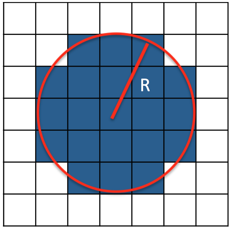
Figure 1: An example of a 2D GP stencil with a radius $R$. It consists of a collection grid cells $I_{i_{k}}$ (blue cells) that are included in a multidimensional blocky sphere of a radius $R$ from the local cell $I_{i_{0}}$, in which the GP interpolation/reconstruction takes place.

An important practical feature of the SE covariance function is that it provides its dimensional factorization analytically. Therefore, the volume averages in Eqs. (22) and (23) simplify to iterated integrals, and in fact they can be expressed analytically in terms of a pre-computed list of error functions of arguments proportional to one-dimensional cell center differences. Eqs. (23) and (24) become

$$\mathbf{C}_{kh}=\sqrt{\pi}\left(\ \frac{\ell}{\Delta}\right)^{2} \left\{\left(\frac{\Delta_{kh}+1}{\sqrt{2}\ell/\Delta}\operatorname{erf}\left[\frac{\Delta_{kh}+1}{\sqrt{2}\ell/\Delta}\right]+\frac{\Delta_{kh}-1}{\sqrt{2}\ell/\Delta}\operatorname{erf}\left[\frac{\Delta_{kh}-1}{\sqrt{2}\ell/\Delta}\right]\right)\right.$$

$$+\frac{1}{\sqrt{\pi}} \left.\left(\exp\left[-\frac{(\Delta_{kh}+1)^{2}}{2(\ell/\Delta)^{2}}\right]+\exp\left[-\frac{(\Delta_{kh}-1)^{2}}{2(\ell/\Delta)^{2}}\right]\right)\right.$$

$$-2 \left.\left(\frac{\Delta_{kh}}{\sqrt{2}\ell/\Delta}\operatorname{erf}\left[\frac{\Delta_{kh}}{\sqrt{2}\ell/\Delta}\right]+\frac{1}{\sqrt{\pi}}\exp\left[-\frac{\Delta_{kh}^{2}}{2(\ell/\Delta)^{2}}\right]\right)\right\},$$ (30)

and

$$\mathbf{T}_{*,k}=\sqrt{\frac{\pi}{2}}\frac{\ell}{\Delta}\left\{\operatorname{erf}\left[\frac{\Delta_{k*}+1/2}{\sqrt{2}\ell/\Delta}\right]-\operatorname{erf}\left[\frac{\Delta_{k*}-1/2}{\sqrt{2}\ell/\Delta}\right]\right\},$$ (31)

using the SE kernel, where $\Delta_{kh}=(x_{k}-x_{h})/\Delta$. Other choices of covariance kernel functions are also available stein1999 ; Cressie2015 , while such choices would require numerical approximations for Eqs. (24) and (23), rather than a possible analytical form as in the SE case.

2.5 GP-WENO: New GP-based Smoothness Indicators for Non-smooth Flows

For smooth flows the GP linear prediction in Eq. (25) with the SE covariance kernel Eq. (29) furnishes a high-order GP reconstruction algorithm without any extra controls on numerical stability. However, for non-smooth flows the unmodified GP-SE reconstruction suffers from unphysical oscillations that originate at discontinuities such as shocks. To handle flows with discontinuities a hybrid method can be implemented using a shock detector (see balsara1999 ) to switch to a lower order piecewise linear method from the GP reconstruction when there is a shocked cell in the stencil. We have implemented such a hybrid method and found that it works well in general for problems with shocks, such as the Sod shock tube problem. However, we noticed that it fails to capture features in flow regions that contain a transition from smooth flow to a shock, producing unphysical oscillations there.

To ultimately resolve such issues with non-smooth flows we adopt the principal idea of employing the nonlinear weights in the Weighted Essentially Non-oscillatory (WENO) methods jiang1996efficient , by which we adaptively change the size of the reconstruction stencil to avoid interpolating through a discontinuity, while retaining high-order properties in smooth flow regions. A traditional WENO takes the weighted combination of candidate stencils based on the local smoothness of the individual sub-stencils. The weights are chosen so that they are optimal in smooth regions, in the sense that they are equivalent to an approximation using the global stencil that is the union of the candidate sub-stencils.

For a stencil $S_{R}$ of a radius $R$, with $2R+1$ points centered at the cell $I_{i}$, we consider $R+1$ candidate sub-stencils $S_{m}\subset S_{R}$, each with $R+1$ points. Similar to the traditional WENO schemes, we subdivide $S_{R}$ given as

$$S_{R}=\bigcup\limits_{m=i-R}^{i+R}I_{m}$$ (32)

into $R+1$ sub-stencils $S_{m}$,

$$S_{m}=\{I_{i-R+m-1},\ldots,I_{i},\ldots,I_{i+m-1}\},\;\;\;m=1,\ldots,R+1.$$ (33)

They satisfy

$$S_{R}=\bigcup\limits_{m=1}^{R+1}S_{m},\mbox{ and }I_{i}=\bigcap\limits_{m=1}^{R+1}S_{m}.$$ (34)

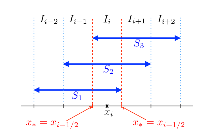
Figure 2: A schematic example of the 5-point GP stencil with $R=2$ centered at $x_{i}$. Two grid locations indicated as $x_{*}$ are the target locations where we seek high-order GP approximations of pointwise value (e.g., $\rho_{*}$) using the given cell-centered volume average data nearby (e.g., $\langle{\rho}_{s}\rangle$, $s=i-2,\dots,i+2$).

Using Eq. (25) on each sub-stencil $S_{m}$, the GP approximation for a pointwise value at a cell location $x_{*}$ from the $m$-th sub-stencil $S_{m}$ is

$$\tilde{f}_{*}^{m}=f_{0}+\mathbf{z}^{T}_{m}(\mathbf{G}_{m}-f_{0}\mathbf{1}_{R+1}).$$ (35)

On the other hand, from the global $2R+1$ stencil $S_{R}$ we also have a pointwise GP approximation at the same location

$$\tilde{f}_{*}=f_{0}+\mathbf{z}^{T}(\mathbf{G}-f_{0}\mathbf{1}_{2R+1}).$$ (36)

Here, the cell location “$*$” is where we want to obtain a desired high-order reconstruction from GP, e.g., the cell interface $x_{*}=x_{i\pm 1/2}$ is of particularly of interest to the Riemann problems in our case. Further, $f_{0}$ is a constant mean function that is the same over all the candidate sub-stencils, $\mathbf{z}^{T}_{m}=\mathbf{T}_{*,m}\mathbf{C}^{-1}_{m}$ is the $(R+1)$-dimensional vector of weights, $\mathbf{G}_{m}$ is the $(R+1)$-dimensional vector of volume averaged data on $S_{m}$ (e.g., the volume averaged densities), and $\mathbf{1}_{R+1}=[1,\ldots,1]^{T}$ is the $(R+1)$-dimensional one-vector. Likewise, $\mathbf{z}^{T}=\mathbf{T}_{*}\mathbf{C}^{-1}$, $\mathbf{G}$, and $\mathbf{1}_{2R+1}$ are $(2R+1)$-dimensional vectors defined in the same way.

We now take the weighted combination of these GP approximations as our final reconstructed value

$$\tilde{f}_{*}=\sum_{m=1}^{R+1}\omega_{m}\tilde{f}_{*}^{m}.$$ (37)

As in the traditional WENO approach, the weights $\omega_{m}$ should reduce to some optimal weights $\gamma_{m}$ in smooth regions such that the approximation in Eq. (37) gives the GP approximation over the global $2R+1$ point stencil. The $\gamma_{m}$’s then should satisfy

$$\mathbf{z}^{T}(\mathbf{G}-f_{0}\mathbf{1}_{2R+1})=\sum_{m=1}^{R+1}\gamma_{m}\mathbf{z}^{T}_{m}(\mathbf{G}_{m}-f_{0}\mathbf{1}_{R+1}),$$ (38)

where $\boldsymbol{\gamma}=[\gamma_{1},\dots,\gamma_{R+1}]^{T}$ is given by the solution to the $(R+1)\times(2R+2)$ overdetermined system

$$\left(\begin{array}[]{c}\mathbf{M}\\ \sum_{m=1}^{R+1}f_{0}\mathbf{z}^{T}_{m}\cdot\mathbf{1}_{R+1}\end{array}\right)\boldsymbol{{\gamma}}=\left(\begin{array}[]{c}\mathbf{z}\\ f_{0}\mathbf{z}\cdot\mathbf{1}_{2R+1}\end{array}\right).$$ (39)

The columns of the matrix $\mathbf{M}$ are given by

$$\mathbf{M}_{km}=\left\{\begin{array}[]{cl}\mathbf{z}^{T}_{k,m}&\text{if }I_{k}\in S_{m},\\ 0&\text{otherwise}.\end{array}\right.$$ (40)

The optimal weights $\gamma_{m}$ then depend on the choice of kernel function, but as with the vectors of GP weights, $\mathbf{z}$ and $\mathbf{z}_{m}$, $\gamma_{m}$ need only be computed once. We take the $\gamma_{m}$’s as the least squares solution to the overdetermined system in Eq. (39), which can be determined numerically.

It remains to describe the non-linear weights $\omega_{m}$ in Eq. (37). Again, these should reduce to the optimal weights in smooth regions, but more importantly, they need to serve as an indicator of the quality of data on the sub-stencil $S_{m}$. We adopt the same weights as in the WENO-JS methods jiang1996efficient :

$$\omega_{m}=\frac{\tilde{\omega}_{m}}{\sum_{s}\tilde{\omega}_{s}},\mbox{ where }\tilde{\omega}_{m}=\frac{\gamma_{m}}{(\epsilon+\beta_{m})^{p}},$$ (41)

where we set $p=1$ and $\epsilon=10^{-36}$ for our test results. These weights are based on the so-called smoothness indicators $\beta_{m}$, for each stencil. In modern WENO schemes the smoothness indicators are calculated as the $L_{2}$-norm of the reconstructed polynomial on each ENO stencil $S_{m}$. We wish to construct a new class of smoothness indicators that fits within the GP framework.

To begin with, we give a brief description on the eigenfunction analysis of covariance kernels. Gaussian process regression, as described in Section 2, can be equivalently viewed as Bayesian linear regression using a possibly infinite number of basis functions. One choice of basis functions is the eigenfunctions, $\phi_{i}(\cdot)$, $i=1,\dots,n$, of the covariance kernel function, $k$. By definition each eigenfunction $\phi_{i}$ satisfies

$$\int k(x,x^{\prime})\phi_{i}(x)d\mu(x)=\lambda_{i}\phi_{i}(x^{\prime}).$$ (42)

The eigenpair $(\phi_{i},\lambda_{i})$ consists of the eigenfunction and the eigenvalue of the covariance kernel function $k$ with respect to the measure $\mu$ bishop2007pattern ; rasmussen2005 .

Of interest is when there is a non-negative function $p(x)$ called the density of the measure $\mu$ so that the measure may be written as $d\mu(x)=p(x)dx$. We can approximate the integral in Eq. (42) by choosing $n$ finite sample points, $x_{l}$, $l=1,\dots,n$, from $p(x)$ on some stencil, which gives

$$\lambda_{i}\phi_{i}(x^{\prime})\simeq\frac{1}{n}\sum_{l=1}^{n}k(x_{l},x^{\prime})\phi_{i}(x_{l}).$$ (43)

Plugging in $x^{\prime}=x_{l}$ into Eq. (43) for $l=1,\dots,n$ gives the matrix eigenproblem

$$\mathbf{K}\mathbf{v}_{i}=n\lambda_{i}\mathbf{v}_{i},$$ (44)

where $\mathbf{K}$ is an $n\times n$ Gram matrix with entries $\mathbf{K}_{ij}=k(x_{i},x_{j})$, and $n\lambda_{i}$ is the $i$-th matrix eigenvalue associated with the normalized $n$-dimensional eigenvector $\mathbf{v}_{i}$ satisfying $\mathbf{v}_{i}^{T}\mathbf{v}_{j}=\delta_{ij}$. We see that $\phi_{i}(x_{j})\sim\sqrt{n}\mathbf{e}_{j}\cdot\mathbf{v}_{i}$ where $\mathbf{e}_{j}$ is the $j$-th unit vector, and we get the $\sqrt{n}$ factor from differing normalizations of the eigenvector and eigenfunction. This eigendecomposition of the covariance matrix, when viewed as a principal component analysis (PCA) bishop2007pattern ; rasmussen2005 , can be thought of as decomposing the covariance into the various variational modes that can be represented on the $n$ sample points. For more discussion of eigenfunction analysis of covariance kernels we refer readers to Section 4.3 of rasmussen2005 ; Section 12.3 of bishop2007pattern .

A set of $n$ samples of a function $f(x)$, denoted as

$$\mathbf{f}=[f(x_{1}),f(x_{2}),\dots,f(x_{n})]^{T},$$ (45)

evaluated at the points $x_{l},\,l=1,\dots,n$ as in Eq. (43), can be expanded in the eigenbasis in (44) as

$$\mathbf{f}=\sum_{i=1}^{n}\alpha_{i}\mathbf{v}_{i}.$$ (46)

We can then define a norm in the Hilbert space of functions using the inner product of the function in the reproducing kernel Hilbert space (RKHS) defined by the kernel function $k(x,x^{\prime})$ rasmussen2005 ,

$$\|f\|^{2}_{\mathcal{H}}=<f,f>_{\mathcal{H}}=\sum_{i=1}^{n}\frac{\alpha_{i}^{2}}{\lambda_{i}}.$$ (47)

In this expression for the norm $\|f\|^{2}_{\mathcal{H}}$, the relative weight of a given mode in the data $\mathbf{f}$ is inversely weighted by the eigenvalue $\lambda_{i}$. The SE kernel has a native Hilbert space of $C^{\infty}$ functions, and assigns relatively small eigenvalues to eigenfunctions that vary rapidly on short length scales. The quantity $\|f\|^{2}_{\mathcal{H}}$ thus contains large additive terms when the data embodies a discontinuity, while data corresponding to smooth regions produces smaller additive terms. This suggests that we may use $\|f\|^{2}_{\mathcal{H}}$ to supply the basis for a GP-based smoothness indicator in the non-linear weights in Eq. (41).

We now use the above discussion of the eigendecomposition to focus on the practical implementation of our new GP-based smoothness indicators. It remains to specify how to obtain the $\alpha_{i}$’s from the volume averaged data $\mathbf{G}_{m}$ on the sub-stencil $S_{m}$. Using the notation ‘$m$’ to denote the objects restricted on each $S_{m}$, the eigenproblem in Eq. (44) on $S_{m}$ can be written as

$$\mathbf{K}^{m}\mathbf{v}_{i}^{m}=\lambda_{i}^{m}\mathbf{v}_{i}^{m},\,i=1,\dots,R+1,$$ (48)

where $\mathbf{K}^{m}$ is the $(R+1)\times(R+1)$ sub-matrix. Note that here we are using the pointwise covariance kernel $\mathbf{K}^{m}$ from Eq. (29) rather than the integrated covariance kernel $\mathbf{C}^{(m)}$ from Eq. (23). In this way we obtain the eigenpair $(\lambda_{i}^{m},\mathbf{u}_{i}^{m})$ that is consistent with providing $\beta_{m}$ which is to measure smoothness of pointwise values $\tilde{f}^{m}_{*}=\tilde{f}^{m}(x_{*})=\tilde{f}^{m}(x_{i\pm\frac{1}{2}})$ in Eq. (37).

Consider a $(R+1)$-dimensional cell-centered pointwise values

$$\mathbf{f}^{m}=[f^{m}(x_{1}),\dots,f^{m}(x_{R+1})]^{T}.$$ (49)

We can express $\mathbf{f}^{m}$ in the basis $\mathbf{v}_{i}^{m}$ as

$$\mathbf{f}^{m}=\sum_{i=1}^{R+1}\alpha_{i}^{m}\mathbf{v}_{i}^{m},\,\mbox{ for each }m=1,\dots,R+1.$$ (50)

Each element $f^{m}(x_{l})$, $l=1,\dots,R+1$, can be reconstructed from $\mathbf{G}_{m}$, using a zero mean $f_{0}=0$ in Eq. (28), as

$$f^{m}(x_{l})=\mathbf{z}^{T}_{m}(x_{l})\cdot\mathbf{G}_{m},$$ (51)

where $(R+1)$-dimensional vector $\mathbf{z}^{T}_{m}(x_{l})=\mathbf{T}_{l,k}^{m}(\mathbf{C}^{m})^{-1}$, $k=1,\dots,R+1$, and

$$\mathbf{G}_{m}=[\langle q_{1}\rangle,\dots,\langle q_{R+1}\rangle]^{T}.$$ (52)

Here $\mathbf{T}_{l,k}^{m}$ is the prediction vector (Eq. (31)) over the sub-stencil $S_{m}$ evaluating the covariance between the cell average values $\langle q_{k}\rangle$, $k=1,\dots,R+1$, and the pointwise value $q_{l}$ evaluated at each $x_{l}\in S_{m}$.

Obtaining $\alpha_{i}^{m}$ is straightforward from Eq. (50). Using $(\mathbf{v}_{j}^{m})^{T}\mathbf{v}_{i}^{m}=\delta_{ji}$,

$$\alpha_{i}^{m}=(\mathbf{v}_{i}^{m})^{T}\cdot\mathbf{f}^{m}.$$ (53)

Finally for each $m$ we have our new GP-based smoothness indicators for the data on the sub-stencil $S_{m}$ given by

$$\beta_{m}=\sum_{i=1}^{R+1}\frac{\left(\alpha_{i}^{m}\right)^{2}}{\lambda^{m}_{i}}.$$ (54)

The computational efficiency of Eqs. (51) and (53) can be improved by introducing vectors $\mathbf{P}^{m}_{i}$ defined as

$$\mathbf{P}^{m}_{i}=(\mathbf{v}^{m}_{i})^{T}\cdot\mathbf{Z}^{T}_{m},$$ (55)

where the $l$-th column of the matrix $\mathbf{Z}_{m}$ is given by $\mathbf{z}_{m}(x_{l})$, $l=1,\dots,R+1$. In this way we precompute $\mathbf{P}^{m}_{i}$ which can directly act on the volume average quantities of $\mathbf{G}_{m}$, by which the $\alpha_{i}^{m}$’s are given by

$$\alpha^{m}_{i}=\mathbf{P}^{m}_{i}\cdot\mathbf{G}_{m}.$$ (56)

To see the computational efficiency in comparison, in Appendix B we provide operation counts of the two approaches referred to as “Option 1” with solving Eqs. (51) and (53), and “Option 2” with solving Eqs. (55) and (56). Option 2 was used for the results shown in Section 4.

It is noteworthy that there is an alternative interpretation of Eq. (54) available in terms of the log likelihood function. Notice that Eq. (54) can be written as a quadratic form

$$(\mathbf{f}^{m})^{T}(\mathbf{K}^{m})^{-1}\mathbf{f}^{m},$$ (57)

which is again equivalent to

$$-2\ln{P(\mathbf{f}^{m})}+C,$$ (58)

assuming $f_{0}=0$ in the relation in Eq. (5) and $C=\ln(\det{|\mathbf{K}|}^{-1})+N\ln(2\pi)$. The analogy between Eq. (54) and Eq. (57) can be proved easily if we realize that the matrix $\mathbf{K}^{m}$ can be expressed as

$$\mathbf{K}^{m}=\sum_{i=1}^{R+1}\lambda_{i}^{m}\mathbf{v}_{i}^{m}(\mathbf{v}_{i}^{m})^{T},$$ (59)

and hence

$$(\mathbf{K}^{m})^{-1}=\sum_{i=1}^{R+1}\frac{1}{\lambda_{i}^{m}}\mathbf{v}_{i}^{m}(\mathbf{v}_{i}^{m})^{T}.$$ (60)

The result follows easily by plugging Eqs. (50) and (60) into Eq. (57) to get Eq. (54). So the statement $\beta_{m}$ is large in this sense is analogous to the statement that the likelihood of $\mathbf{f}^{m}$ is small. The statistical interpretation is that short length-scale variability in $\mathbf{f}^{m}$ make its data unlikely according to the smoothness model represented by $\mathbf{K}^{m}$.

It was observed by Jiang and Shu jiang1996efficient that it is critically important to have appropriate smoothness indicators so that in smooth regions the non-linear weights reproduce the optimal linear weights to the design accuracy in order to maintain high order of accuracy in smooth solutions. Typically this is shown by Taylor expansion of smoothness indicators in Eq. (41). Here we propose to calculate the eigendecomposition in Eq. (44) numerically, and therefore we don’t provide a mathematical proof for the accuracy of our new smoothness indicators. Nonetheless we observe the expected high order convergence expected from the polynomial WENO reconstructions on the equivalent stencils in numerical experiments provided in Section 4.2.

3 Steps in GP-SE Algorithm for 1D FVM

Before we present the numerical results of the GP reconstruction algorithms detailed in the above, we give a quick summary on the step-by-step procedure for 1D simulations with FVM. The 1D algorithm of GP outlined above can be summarized as below:

1. Pre-Simulation: The following steps are carried out before starting a simulation, and any calculations therein need only be performed once, stored, and used throughout the actual simulation.

   1. Configure computational grid: Determine a GP stencil radius $R$ as well as choose the size of the hyperparameter $\ell$. This determines the SE kernel function in Eq. (29) as well as the global and candidate stencils in Eqs. (32) & (33).

   2. Compute GP weights: Compute the covariance matrices, $\mathbf{C}$ and $\mathbf{C}_{m}$ (Eq. (23)) on the stencils $S_{R}$ and each of $S_{m}$ as well as the prediction vectors, $\mathbf{T}_{*}$ (Eq. (24)). The GP weight vectors, $\mathbf{z}^{T}=\mathbf{T}_{*}\mathbf{C}^{-1}$, on each of the stencils can then be stored for use in the GP reconstruction. The columns of the matrices $\mathbf{Z}_{m}$, $\mathbf{z}_{m}(x_{l})$’s, should be computed here for use in step (d). It is crucial in this step as well as in Step (c) to use the appropriate floating point precision to prevent the covariance matrix $\mathbf{C}$ from being numerically singular. This is discussed in more detail in Section 4.2. We find that double precision is suitable up to condition numbers $\kappa\sim 10^{8}$, whereas quadruple precision allows up to $\kappa\sim 10^{18}$. The standard double precision is used except for Step (b) and Step (c).

   3. Compute linear weights: Use the GP weight vectors to calculate and store the optimal linear weights according to Eq. (39).

   4. Compute kernel eigensystem: The eigensystem for the covariance matrices used in GP-WENO are calculated using Eq. (44). The matrices, $\mathbf{C}_{m}$, are the same on each of the candidate stencils in the GP-WENO scheme presented here, so only one eigensystem needs to be determined. This eigensystem is then used to calculate and store the vectors $\mathbf{P}^{(m)}_{i}$ in Eq. (55) for use in determining the smoothness indicators in the reconstruction Step 2.

   At this point, before beginning the simulation, if quadruple precision was used in Step (b) and Step (c) the GP weights and linear weights can be truncated to double precision for use in the actual reconstruction step.

2. Reconstruction: Start a simulation. Choose $f_{0}$ according to Eq. (65) or simply set to zero. The simplest choice $f_{0}=0$ gives good results in practice and yields $\bar{\mathbf{G}}=0$ in Eq. (25). At each cell $x_{i}$, calculate the updated posterior mean function $\tilde{f}_{*}$ in Eq. (25) as a high-order GP reconstructor to compute high-order pointwise Riemann state values at $x_{*}=x_{i\pm 1/2}$ using each of the candidate stencils. The smoothness indicators (Eq. (54)) are calculated using the eigensystem from Step (d) and, in conjunction with the linear weights from Step (c), form the non-linear weights (Eq. (41)). Then take the convex combination according to Eq. (37).

3. Calculate fluxes: Solve Riemann problems at cell interfaces using the high-order GP Riemann states in Step 2 as inputs.

4. Temporal update: Update the volume-averaged solutions $\langle q_{i}\rangle$ from $t^{n}$ to $t^{n+1}$ using the Godunov fluxes from Step 3.

4 Numerical Results

Here we present numerical results using the GP-WENO reconstructions with stencil radii $R=1,2,3$ (denoted as GP-R1, GP-R2, GP-R3 respectively), described in Section 2.5, applied to the 1D compressible Euler equations and the 1D equations of ideal magnetohydrodynamics (MHD). The GP-WENO method will be the default reconstruction scheme hereafter.

We compare the solutions of GP-WENO with the fifth-order WENO (referred to as WENO-JS in what follows) FVM jiang1996efficient ; shu2009high , using the same non-linear weights in Eq. (41). The only difference between using WENO-JS and GP-R2 is the use of polynomial based reconstruction and smoothness indicators shu2009high for WENO-JS, and the use of Gaussian process regression with the new GP-based smoothness indicators for GP. A fourth-order TVD Runge-Kutta method shu1988tvd for temporal updating, and the HLLC li2005hllc ; toro1994restoration or Roe roe1981approximate Riemann solvers are used throughout.

4.1 Performance Comparison

We first present a performance comparison for the proposed GP scheme and the WENO-JS scheme summarized in Table 1. We see that the cost of the GP-R2 and WENO-JS methods are very nearly the same, operating on the same stencils. The minor difference can be attributed to the new GP based smoothness indicators. It can be seen in Eq. (54) the GP smoothness indicators can be written as the sum of $R+1$ perfect squares, which is three terms for each $\beta_{m}$ for GP-R2, meanwhile the smoothness indicators for WENO-JS contain only two terms (i.e., the first and second derivatives of the second-degree ENO polynomials $p_{m}(x)$). The additional cost is offset by a significant advantage in smooth regions near discontinuities over the WENO-JS scheme, which is discussed in Section 4.3.

Scheme	Speedup
GP-R1	0.8
GP-R2	1.0
GP-R3	1.4
WENO-JS	0.9

Table 1: Shown is the relative time to solution for the four methods considered, all normalized to the GP-R2 time.

4.2 1D Smooth Advection

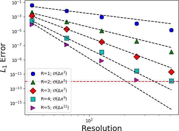
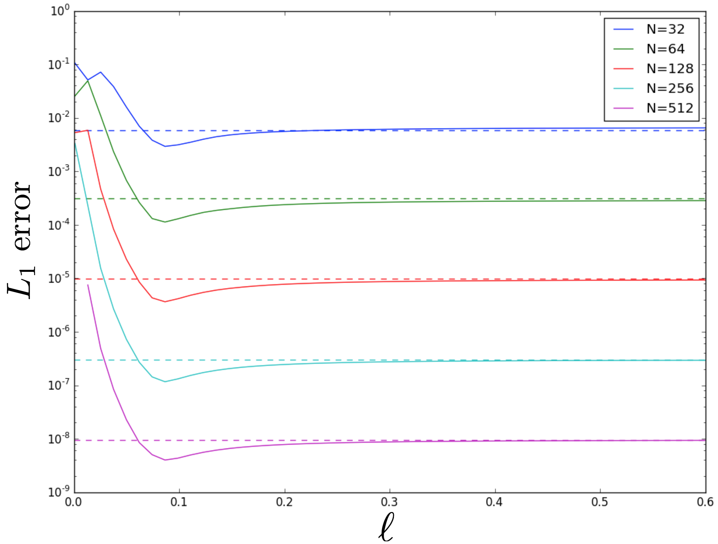
Figure 3: (a) Convergence for smooth Gaussian density advection using different GP stencil radii, all using the length scale $\ell=0.1$ and the HLLC Riemann solver with $C_{\text{cfl}}=0.8$. Black dotted lines show $2R+1$ convergence rates, ranging from 3rd-order ($R=1$) to 11th-order ($R=5$). Red dotted line represents a plateau at an $L_{1}$ of $10^{-12}$ where a large condition number of the covariance matrix is obtained and no further accuracy is achievable. (b) $L_{1}$ errors as a function of the hyperparameter $\ell$, using $R=2$. Dotted lines are the error for fifth-order WENO-JS method on the same stencil.

The test considered here involves the passive advection of a Gaussian density profile. We initialize a computational box on [0,1] with periodic boundary conditions. The initial density profile is defined by $\rho(x)=1+e^{-100(x-x_{0})^{2}}$, with $x_{0}=0.5$, with constant velocity, $u=1$, and pressure, $P=1/\gamma$. The specific heat ratio is chosen to be $\gamma=5/3$. The resulting profile is propagated for one period through the boundaries. At $t=1$, the profile returns to its initial position at $x=x_{0}$, any deformation of the initial profile is due to either phase errors or numerical diffusion. We perform this test using a length hyperparameter of $\ell=0.1$ for stencil radii $R=1,2,3,4$ and $5$, with a fixed Courant number, $C_{\text{cfl}}=0.8$ and vary the resolution of computational box, with $N=32,64,128,256$ and $512$.

The results of this study are shown in Fig. 3. From these numerical experiments, GP reconstruction shows a convergence rate that goes as the size of the stencil, $2R+1$. Note that this convergence rate $2R+1$ of GP is equivalent to the convergence rate $2r-1$ of a classic WENO method for a same size of stencil. In the classic WENO method, the notation $r$ represents the order (not degree) of polynomials on $S_{m}$ which require $r$ cells on each $S_{m}$, totaling $2r-1$ cells on $S_{R}$. This implies $2r-1=2R+1$, or $R=r-1$. For example GP-R2 converges at fifth-order on the stencil $S_{R}=S_{2}$ that has five cells, so does WENO-JS with three third-order ENO polynomials (i.e., $r=3$) on the same 5-point stencil.

In Fig. 3 the $L_{1}$ error plateaus out at an $\sim 10^{-12}$ which is a few orders of magnitude greater than the standard IEEE double-precision, $\sim 10^{16}$. This happens because at high resolution the length hyperparameter, $\ell$, becomes very large relative to the grid spacing, $\Delta$. The covariance matrix, $\mathbf{C}$ given in Eq. (2.4) becomes nearly singular in the regime $\ell/\Delta\gg 1$, yielding very large condition numbers for $\mathbf{C}$. We find the plateau in the $L_{1}$ error occurs for condition numbers, $\kappa\sim 10^{18}$, corresponding to the point where the errors in inverting $\mathbf{C}$ in Eq. (25) begin to dominate. This implies that the choice of floating-point precision has an immense impact on the possible $\ell/\Delta$, and a proper floating-point precision needs to be chosen in such a way that the condition number errors do not dominate. As mentioned in Section 2.4, SE suffers from singularity when the size of the dataset grows. The approach that enabled to produce the results in Fig. 3 is to utilize quadruple-precision only for the calculation of $\mathbf{z}^{T}=\mathbf{T}_{*}^{T}\mathbf{C}^{-1}$ in Eq. (25). Otherwise, the plateau would appear at a much higher $L_{1}$ error $\sim 10^{-7}$ with double-precision, producing undesirable outcomes for all forms of grid convergence studies. This corresponds to condition numbers $\kappa\sim 10^{8}$, and as a point of reference, the breakdown starts to occur for $\ell/\Delta>48$ using a GP radius $R=2$. Since $\mathbf{z}^{T}$ needs to be calculated only once, before starting the simulation, it can then be truncated to double-precision for use in the actual reconstruction procedure. There are only four related small subroutines that need to be compiled with quadruple-precision in our code implementation. The overall performance is not affected due to this extra precision handling. It should be noted that this extra precision handling is necessary for the purpose of a grid convergence study from the perspective of CFD applications.

The correlational length hyperparameter $\ell$ provides an additional avenue to tune solution accuracy that is not present in polynomial-based methods. Fig. 3 shows how the GP errors with $R=2$ in the smooth-advection problem changes with the choice of $\ell$, compared with the error from a fifth-order WENO-JS + RK4 solution (denoted in dotted lines). At large $\ell$ the errors become roughly the same as in WENO-JS, and at small $\ell$ the errors become worse. The error finds a minimum at a value of $\ell$ near the half-width of the Gaussian density profile. This is in line with the idea that the optimal choice of $\ell$ should match the physical length scale of the feature being resolved. We will report new strategies on this topic in our future papers.

4.3 1D Shu-Osher Shock Tube Problem

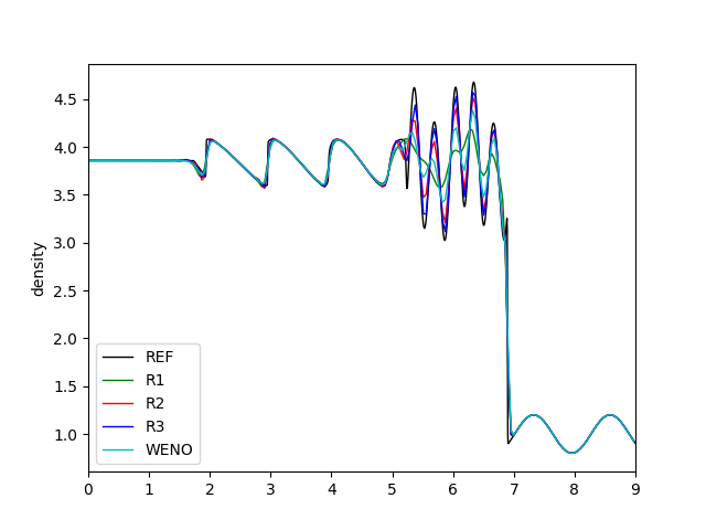
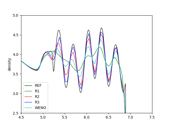
Figure 4: The Shu-Osher problem. Density profiles at $t=1.8$ computed using three different GP stencil radii ($R=1,2,3$) on a 200 grid resolution with $C_{\text{cfl}}=0.8$. All GP calculations use $\ell/\Delta=6$ and the HLLC Riemann solver. The reference solution is obtained using WENO-JS on a 2056 grid resolution. 4 shows a closeup view of the post shock features.

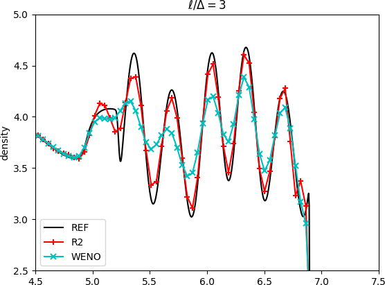
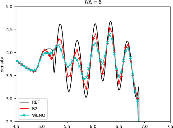
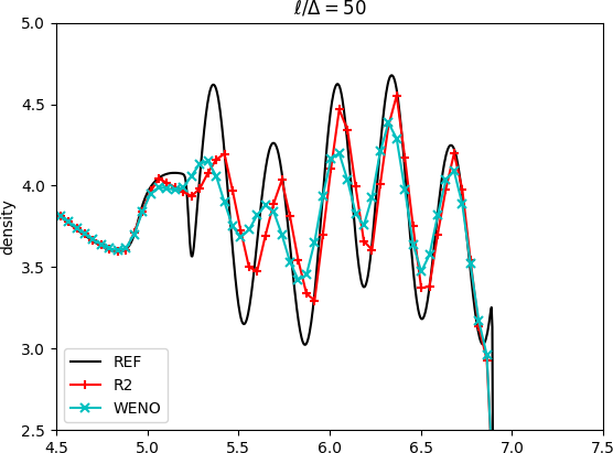
Figure 5: Closeup view of the post shock features as in Fig. 4 using $N=200$ for WENO-JS and GP-R2 (a) with $\ell/\Delta=3$, (b) with $\ell/\Delta=6$, and (c) with $\ell/\Delta=50$. The reference solution is calculated using WENO-JS on 2056 grid resolution.

The second test is the Shu-Osher problem Shu1989 to test GP’s shock-capturing capability as well as to see how well GP can resolve small-scale features in the flow. The test gives a good indication of the method’s numerical diffusivity, and it has been a popular benchmark to demonstrate numerical errors of a given method. In this problem, a (nominally) Mach 3 shock wave propagates into a constant density field with sinusoidal perturbations. As the shock advances, two sets of density features appear behind the shock. One set has the same spatial frequency as the unshocked perturbations, while in the second set the frequency is doubled and follows more closely behind the shock. The primary test of the numerical method is to accurately resolve the dynamics and strengths of the oscillations behind the shock.

The results are shown in Fig. 4. The solutions are calculated at $t=1.8$ using a resolution of $N=200$ and are compared to a reference solution resolved on $N=2056$. It is evident that the GP solution using $R=3$ provides the least diffusive solution of the methods shown, especially in capturing the amplitude of the post-shock oscillations in Fig. 4. Of the two fifth-order methods, GP-R2 and WENO-JS, the GP solution has slightly better amplitude in the post-shock oscillations compared to the WENO-JS solution, consistent with what is observed in Section 4.2 for the smooth advection problem.

The results in Section 4.2 suggest that the choice of $\ell$ should correspond with a length scale characteristic of the flow for optimal performance. Fig. 5 compares the post shock features on the same grid for the WENO-JS method and the GP-R2 method with $\ell/\Delta=3,6$ and $50$. Here $\ell/\Delta=3$ is roughly a half wavelength of the oscillations, and the GP-R2 method clearly gives a much more accurate solution compared to the WENO-JS solution. Just as can be seen in Fig. 3, $\ell/\Delta$ much larger than the characteristic length yields a solution much closer to that of WENO-JS. From Fig. 3 we expect that the GP reconstructions in Eq. (35) should approach the WENO-JS reconstructions in smooth regions for $\ell\gg\Delta$. However, we see that the new GP based smoothness indicators allow for the amplitudes near the shock to be better resolved. This reflects a key advantage of the proposed GP method over polynomial-based high-order methods. The additional flexibility afforded by the kernel hyperparameters in GP, allowing for solution accuracy to be tuned to the features that are being resolved. Only at larger values of $\ell$ does the model become fully constrained by the data in GP, whereas the interpolating polynomials used in a classical WENO are always fully constrained by design. Analogously in the RBF theory, the the shape parameters $\epsilon_{j}$ plays an important role in the similar context of accuracy and convergence. Several strategies have been studied recently for solving hyperbolic PDEs bigoni2016adaptive ; guo2017rbf ; jung2010recovery .

4.4 The Sod Shock Tube Test

The shock tube problem of Sod sod1978survey has been one of the most popular 1D tests of a code’s ability to handle shocks and contact discontinuities. The initial conditions, on the domain $[0,1]$, are given by the left and right states

$$(\rho,u,p)=\left\{\begin{array}[]{lr}(1,0,1),&x<0.5,\\ (0.125,0,0.1),&x>0.5,\end{array}\right.$$ (61)

with the ratio of specific heats $\gamma=1.4$. Outflow boundary conditions are imposed at $x=0$ and $x=1$. The results are shown in Fig. 6.

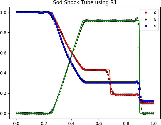
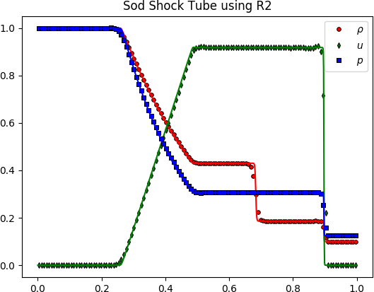
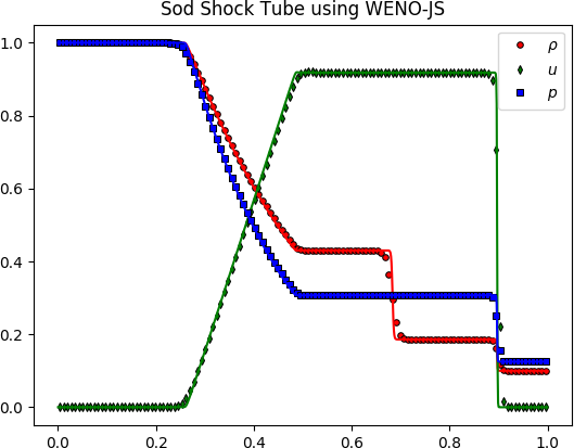
Figure 6: The Sod shock tube problem at $t=0.2$. (a) GP with stencil radius $R=1$, (b) GP with stencil radius $R=2$, (c) GP with stencil radius $R=3$, and (d) WENO-JS, all using 128 grid points with $C_{\text{cfl}}=0.8$. All GP calculations use $\ell/\Delta=12$ and the HLLC Riemann solver. Solid lines show a reference solution computed using WENO-JS on 1024 grid points.

All of the GP-WENO schemes correctly predicts the nonlinear characteristics of the flow including the rarefaction wave, contact discontinuity and the shock. The solution using GP-R2 is very comparable to the WENO-JS solution using the same 5-point stencil. As expected, the GP-R1 solution smears out the most at both the shock and the contact discontinuity, and at the head and tail of the rarefaction. The 7th order GP-R3 also successfully demonstrates that its shock solution is physically correct without triggering any unphysical oscillation. Somewhat counter intuitively from the perspective of 1D polynomial schemes, the smallest stencil GP-R1 shows the most oscillations near the shock. This happens because the eigendecomposition of the kernel in Eq. (44) used in the calculation the smoothness indicators for Eq. (54) better approximates $\|f\|_{\mathcal{H}}^{2}$ as the size of the stencil increases. Recall that the eigenexpansion of the kernel function in Eq. (42) can contain an infinite number of eigenvalues, and so can $\|f\|_{\mathcal{H}}^{2}$ and the sum in Eq. (47). The finite approximation to the eigensystem and subsequently $\|f\|_{\mathcal{H}}^{2}$ then becomes better as the smallest coefficient $\alpha_{i}$ goes to zero. Then for GP, the $\beta_{m}$’s best indicate the smoothness on larger sized stencils.

4.5 The Einfeldt Strong Rarefaction Test

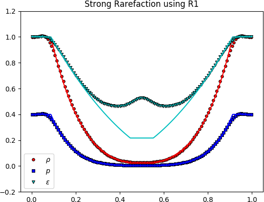
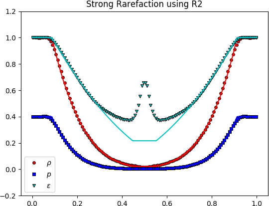
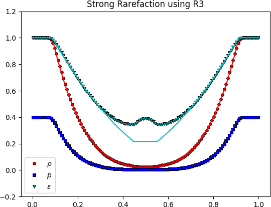
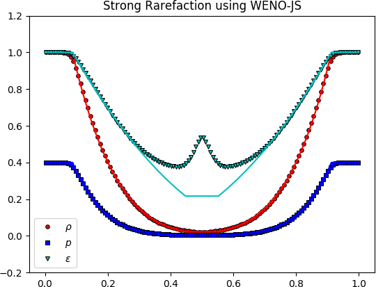
Figure 7: The Einfeldt strong rarefaction test at $t=0.15$. (a) GP with stencil radius $R=1$, (b) GP with stencil radius $R=2$, (c) GP with stencil radius $R=3$, and (d) WENO-JS, all using 128 grid points with $C_{\text{cfl}}=0.8$. All GP calculations use $\ell/\Delta=12$ and the HLLC Riemann solver. Solid lines show the exact solution.

First described by Einfeldt et al. einfeldt1991godunov , this problem tests how satisfactorily a code can perform in a low density region in computing physical variables, $\rho,u,p,\epsilon$, etc. Among those, the internal energy $\epsilon=p/(\rho(\gamma-1))$ is particularly difficult to get right due to regions where the density and pressure are very close to zero. The ratio of these two small values amplifies any small errors in both $\rho$ and $p$, making the errors in $\epsilon$ the largest in general toro2009 . The large errors in $\epsilon$ are apparent for all schemes shown in Fig. 7, where the error is largest around $x=0.5$. It can be observed that the amount of departure in $\epsilon$ from the exact solution (the cyan solid line) decreases as the GP radius $R$ increases. The error in GP-R2 is slightly larger for $\epsilon$ at the center than in WENO-JS. However, the peak becomes considerably smaller in amplitude and becomes slightly flatter as $R$ increases.

4.6 Brio-Wu MHD Shock Tube

Brio and Wu brio1988upwind studied an MHD version of Sod’s shock tube problem, which has since become an essential test for any MHD code. The test has since uncovered some interesting findings, such as the compound wave brio1988upwind , as well as the existence of non-unique solutions torrilhon2003non ; torrilhon2003uniqueness . The results for this test are shown in Fig. 8.

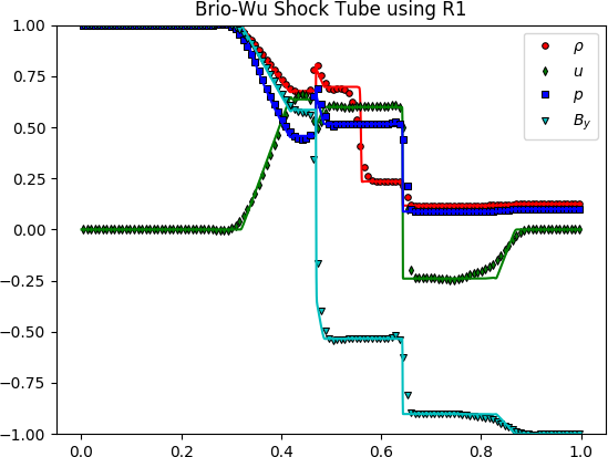
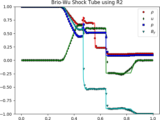
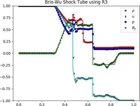
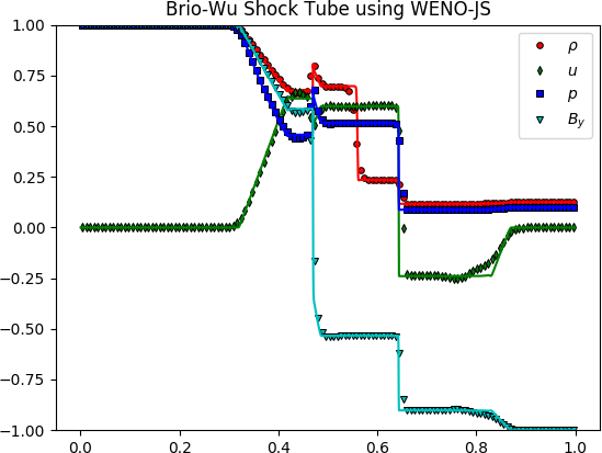
Figure 8: The Brio-Wu shock tube at $t=0.1$. (a) GP with stencil radius $R=1$, (b) GP with stencil radius $R=2$, (c) GP with stencil radius $R=3$, and (d) WENO-JS, all using 128 grid points with $C_{\text{cfl}}=0.8$. All GP calculations use $\ell/\Delta=12$ and the Roe Riemann solver. Solid lines show a reference solution computed using WENO-JS on 1024 grid points.

All of the GP methods are able to satisfactorily capture the MHD structures of the problem. In all methods, including WENO-JS, there are some observable oscillations in the post shock regions. Lee in lee2011upwind showed that these oscillations arise as a result of the numerical nature of the slowly moving shock woodward1984numerical controlled by the strength of the transverse magnetic field. As studied by various researchers arora1997postshock ; jin1996effects ; johnsen2008numerical ; karni1997computations ; roberts1990behavior ; stiriba2003numerical , there seems no ultimate fix for controlling such unphysical oscillations due to the slowly moving shock. Quantitatively, the amount of oscillations differs in different choices of numerical methods such as reconstruction algorithms and Riemann solvers. We see that all of the GP solutions together with the WENO-JS solution feature a comparable level of oscillations. Except for GP-R1, all solutions also suffer from a similar type of distortions in $u$ and $B_{y}$ in the right going fast rarefaction. This distortion as well as the oscillations due to the slowly moving shock seem to be suppressed in the 3rd order GP-R1.

4.7 Ryu and Jones MHD Shock Tubes

Ryu and Jones ryu1994numerical introduced a large set of MHD shock tube problems as a test of their 1D algorithm, that are now informative to run as a code verification. In what follows we will refer to the tests as RJ followed by the corresponding figure from ryu1994numerical in which the test can be found.

4.7.1 RJ1b Shock Tube

Figure 9: The RJ1b MHD shock tube at $t=0.03$. (a) GP with stencil radius $R=1$, (b) GP with stencil radius $R=2$, (c) GP with stencil radius $R=3$, and (d) WENO-JS, all using 128 grid points with $C_{\text{cfl}}=0.8$. All GP calculations use $\ell/\Delta=12$ and the Roe Riemann solver. Solid lines show a reference solution computed using WENO-JS on 1024 grid points.

The first of the RJ shock tubes we consider is the RJ1b problem. This test contains a left going fast and slow shock, contact discontinuity as well as a slow and fast rarefaction. In Fig. 9 that all waves are resolved in the schemes considered.

4.7.2 RJ2a Shock Tube

Figure 10: The RJ2a MHD shock tube at $t=0.03$. (a) GP with stencil radius $R=1$, (b) GP with stencil radius $R=2$, (c) GP with stencil radius $R=3$, and (d) WENO-JS, all using 128 grid points with $C_{\text{cfl}}=0.8$. All GP calculations use $\ell/\Delta=12$ and the HLLC Riemann solver. Solid lines show a reference solution computed using WENO-JS on 1024 grid points.

The RJ2a test provides an interesting test due to its initial conditions producing a discontinuity in each of the MHD wave families. The solution contains both fast- and slow- left and right-moving magnetoacoustic shocks, left- and right-moving rotational discontinuities and a contact discontinuity. Fig. 10 shows that all three of the GP schemes are able to resolve all of these discontinuities. Again we see that the smallest stencil GP-R1 solution contains some oscillations near the shock that are not present in the other GP solutions.

4.7.3 RJ2b Shock Tube

Figure 11: The RJ2b MHD shock tube at $t=0.2$. (a) GP with stencil radius $R=1$, (b) GP with stencil radius $R=2$, (c) GP with stencil radius $R=3$, and (d) WENO-JS, all using 128 grid points with $C_{\text{cfl}}=0.8$. All GP calculations use $\ell/\Delta=12$ and the Roe Riemann solver. Solid lines show a reference solution computed using WENO-JS on 1024 grid points.

The RJ2b shock tube creates a set of a fast shock, a rotational discontinuity and a slow shock moving to the left away from a contact discontinuity, as well as a fast rarefaction, rotational discontinuity and slow rarefaction all moving to the right. What is of interest is that since the waves propagate at almost the same speed, at $t=0.035$ they have still yet to separate much, and so test a codes ability to resolve all of the discontinuities despite their close separation. The results of this test for the methods considered are shown in Fig. 11. At the shown resolution of $N=128$, the contact discontinuity and the slow shock become somewhat smeared together in the GP-R1 solution, while they are better resolved for the other methods, even though there are only couple of grid points distributed over the range of the features.

4.7.4 RJ4a Shock Tube

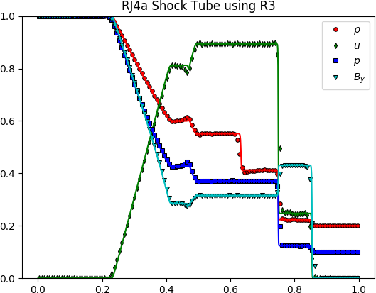
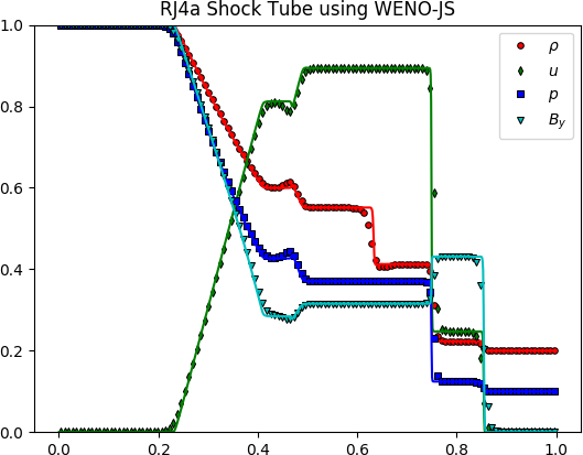
Figure 12: The RJ4a MHD shock tube at $t=0.15$. (a) GP with stencil radius $R=1$, (b) GP with stencil radius $R=2$, (c) GP with stencil radius $R=3$, and (d) WENO-JS, all using 128 grid points with $C_{\text{cfl}}=0.8$. All GP calculations use $\ell/\Delta=12$ and the HLLC Riemann solver. Solid lines show a reference solution computed using WENO-JS on 1024 grid points.

The RJ4a shock tube yields a fast and slow rarefaction, a contact discontinuity, a slow shock, and of particular interest the switch-on fast shock. The feature of the switch-on shock is that the magnetic field turns on in the region behind the shock. As can be seen in Fig. 12, all of the features including the switch-on fast shock are resolved in all methods. We see that GP-R1 smears out the solution not only in resolving discontinuous flow regions, but also in resolving both fast and slow rarefaction waves.

4.7.5 RJ4b Shock Tube

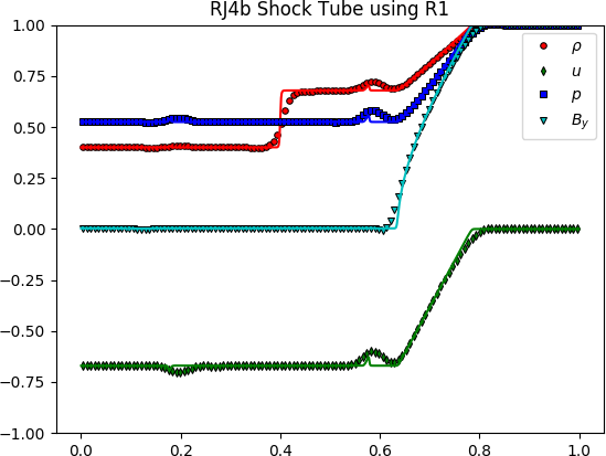
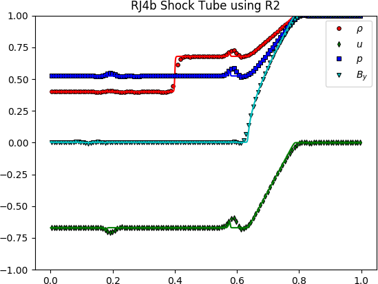
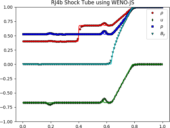
Figure 13: The RJ4b MHD shock tube at $t=0.15$. (a) GP with stencil radius $R=1$, (b) GP with stencil radius $R=2$, (c) GP with stencil radius $R=3$, and (d) WENO-JS, all using 128 grid points with $C_{\text{cfl}}=0.8$. All GP calculations use $\ell/\Delta=12$ and the HLLC Riemann solver. Solid lines show a reference solution computed using WENO-JS on 1024 grid points.

The RJ4b test is designed to produce only a contact discontinuity and a fast right going switch-off fast rarefaction, where the magnetic field is zero behind the rarefaction. We can see in Fig. 13 that both the contact discontinuity and the switch-off rarefaction features are captured in all of the considered methods.

4.7.6 RJ5b Shock Tube

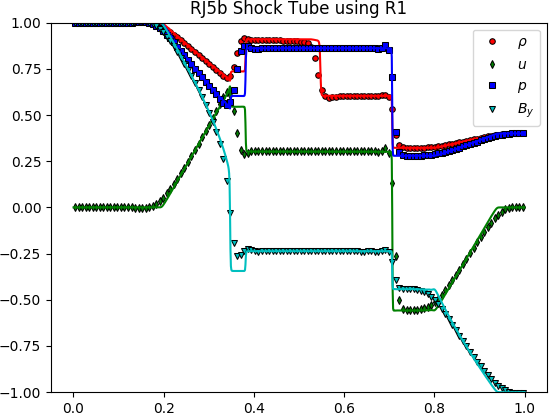
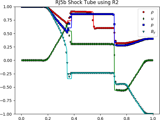
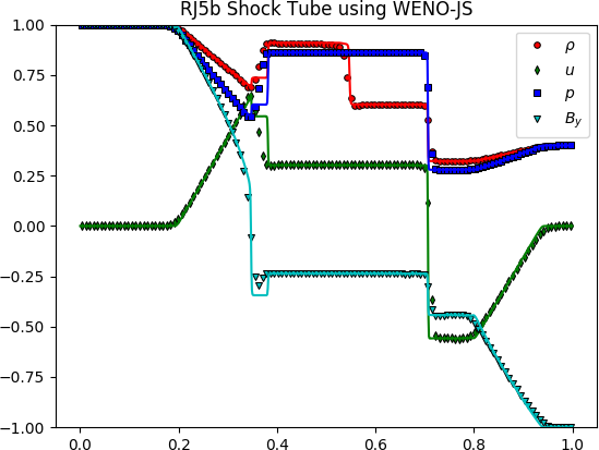
Figure 14: The RJ5b MHD shock tube at $t=0.16$. (a) GP with stencil radius $R=1$, (b) GP with stencil radius $R=2$, (c) GP with stencil radius $R=3$, and (d) WENO-JS, all using 128 grid points with $C_{\text{cfl}}=0.8$. All GP calculations use $\ell/\Delta=12$ and the HLLC Riemann solver. Solid lines show a reference solution computed using WENO-JS on 1024 grid points.

The RJ5b problem is of interest because it produces a fast compound wave, as opposed to the slow compound wave in the Brio-Wu problem, in addition to a left- and right-going slow shock, contact discontinuity and fast rarefaction. At the resolution of $N=128$ used for the results in Fig. 14, the compound wave and one of the slow shocks are smeared together in all the methods tested.

5 Conclusion

We summarize key novel features of the new high-order GP approach presented in this paper.

The new GP approach utilizes the key idea from statistical theory of GP prediction to produce accurate interpolations of fluid variables in CFD applications. We have developed a new set of numerical strategies of GP for both smooth flows and non-smooth flows to numerically solve hyperbolic systems of conservation laws.

The GP methods presented here show an extremely fast rate of solution accuracy in smooth advection problems by controlling a single parameter, $R$. Further, the additional flexibility offered by the GP model approach over the fully constrained polynomial based model through the kernel hyperparameter $\ell$ allows for added tuning of solution accuracy that is not present in traditional polynomial based high-order methods. These parameters allow the GP method to demonstrate variable orders of method accuracy as functions of the size of the GP stencil and the hyperparameter $\ell$ (see Eq. (29)) within a single algorithmic implementation.

The new GP based smoothness indicators introduced here are used to construct non-linear weights that give the essentially non-oscillatory property in discontinuous flows. The new smoothness indicators show a significant advantage over traditional WENO schemes in capturing flow features at the grid resolution near discontinuities.

The GP model, by design, can easily be extended to multidimensional GP stencils. Therefore, GP can seamlessly provide a significant algorithmic advantage in solving the multidimensional PDE of CFD. This “dimensional agnosticism” is unique to GP, and not a feature of polynomial methods. We will report our ongoing developments of GP in multiple spatial dimensions in forthcoming papers.

6 Acknowledgements

The software used in this work was developed in part by funding from the U.S. DOE NNSA-ASC and OS-OASCR to the Flash Center for Computational Science at the University of Chicago.

Appendix A Appendix: Choosing the Optimal Mean $f_{0}$ using the Maximum Likelihood Function

In most practical applications we will not have any prior information on the mean of the function samples. This makes it reasonable to take a zero mean function $f_{0}=0$ if we try to achieve the simplest and most general symmetry of any random samples. However, one can easily determine the best optimal choice of the mean value by maximizing the likelihood of the samples. This can be done by taking the logarithm function of Eq. (5) to first get the $\log$ likelihood function of the function samples $\mathbf{f}=[f(\mathbf{x}_{1}),\dots,f(\mathbf{x}_{N})]^{T}$ that are pointwise,

$$\ln{\mathcal{L}}=\ln{P(\mathbf{f})}=-\frac{1}{2}\left(\mathbf{f}-\bar{\mathbf{f}}\right)^{T}\mathbf{K}^{-1}\left(\mathbf{f}-\bar{\mathbf{f}}\right)-\frac{1}{2}\ln({\det|\mathbf{K}|})-\frac{N}{2}\ln({2\pi}).$$ (62)

To maximize the likelihood, we take the partial derivative of Eq. (62) with respect to $f_{0}$, where $\mathbf{f}=f_{0}\mathbf{1}_{N}$, and set the partial derivative to be zero,

$$0=\frac{\partial\mathcal{L}}{\partial f_{0}} = -\mathbf{f}^{T}\mathbf{K}^{-1}\mathbf{1}_{N}-\mathbf{1}_{N}^{T}\mathbf{K}^{-1}\mathbf{f}+2f_{0}\left(\mathbf{1}_{N}^{T}\mathbf{K}^{-1}\mathbf{1}_{N}\right)$$ (63)

$$= -2\mathbf{f}^{T}\mathbf{K}^{-1}\mathbf{1}_{N}+2f_{0}\left(\mathbf{1}_{N}^{T}\mathbf{K}^{-1}\mathbf{1}_{N}\right),$$

where we used the symmetry of $\mathbf{K}^{-1}$ to get $\mathbf{f}^{T}\mathbf{K}^{-1}\mathbf{1}_{N}=\mathbf{1}_{N}^{T}\mathbf{K}^{-1}\mathbf{f}$. The best optimal value of $f_{0}$ is then given by

$$f_{0}=\frac{\mathbf{1}_{N}^{T}\mathbf{K}^{-1}\mathbf{f}}{\mathbf{1}_{N}^{T}\mathbf{K}^{-1}\mathbf{1}_{N}},$$ (64)

which maximizes the likelihood of the samples in Eq. (5) for the case of interpolations.

In the similar way, we obtain the best optimal value of $f_{0}$ for the case of reconstructions, given as

$$f_{0}=\frac{\mathbf{1}_{N}^{T}\mathbf{C}^{-1}\mathbf{G}}{\mathbf{1}_{N}^{T}\mathbf{C}^{-1}\mathbf{1}_{N}},$$ (65)

where $\mathbf{G}=[\langle q_{1}\rangle,\dots,\langle q_{N}\rangle]^{T}$ contains $N$ volume-averaged values and $\mathbf{C}$ is the integrated kernel in Eq. (23).

These optimal choices of $f_{0}$ are obviously more expensive in computation as they involve local calculations on each GP stencil. In all the tests we presented in this paper we do not see any significant evidence that these optimal values result in any gains in terms of solution accuracy and computational efficiency.

Appendix B Appendix: Operation Counts

We display possible outcomes of computing the GP-based new smoothness indicators in two different approaches described in Section 2.5:

• Option 1: Compute $\alpha_{i}^{m}$ using Eqs. (51) and (53),

• Option 2: Compute $\alpha_{i}^{m}$ using Eqs. (55) and (56).

Consider a 1D domain discretized with $N_{x}$ grid cells. Let’s say we use a GP stencil of a radius $R$, which is subdivided into $R+1$ sub-stencils, $S_{m}$, $m=1,\dots,R+1$. Since the calculations described in Section 2.5 to obtain smoothness indicators need to take place on every cell, there are $N_{x}$ operations involved in total, each of which has $M$ many operation counts at each $S_{R}$ level. Below, we estimate the total number of required operation counts for Option 1 and Option 2.

We first consider Option 1. With a computer code with successive multiplications and additions for a dot product, Eq. (51) involves $R+1$ multiplications and $R+1$ additions for each $m=1,\dots,R+1$. This gives $2(R+1)$ operations for Eq. (51) for each $m$ and $l$. Likewise, we also have $2(R+1)$ operations for Eq. (53) for each $m$ and $i$. As a result, we see there are $2m(R+1)(l+i)$ operations involved on each $S_{R}$. Since there are $N_{x}$ many $S_{R}$ calculations overall, the total number of operations becomes $2m(R+1)(l+i)N_{x}$ per each time step, where $m,i,l=1,\dots R+1$. Assuming there are $M$ time steps required for the run, we require $2m(R+1)(l+i)N_{x}M$ operations in total.

Let us now consider Option 2. A major difference in this case is to realize the fact that Eq. (55) can be pre-computed as soon as the grid is configured. This is because, unlike $f^{m}(x_{l})$ in Eq. (51), the vector $\mathbf{P}^{m}_{i}$ has no dependency on any local data but only on the grid itself, whereby it can be pre-computed and saved for each $m$ and $i$ before evolving each simulation, and reused during the simulation evolutions. The typical operation count for a $(R+1)$-dimensional vector and a $(R+1)\times(R+1)$-dimensional matrix multiplication with successive multiplications and additions is found to be $2(R+1)^{2}$. Hence we see there are $2im(R+1)^{2}$ total operations that can be pre-computed and saved, $m,i=1,\dots,R+1$. Here is an extra operation reduction available by realizing that Eq. (55) is same for all $m$, thereby we have $2i(R+1)^{2}$ total operations for $i=1,\dots,R+1$. Eq. (56) however, needs to be computed locally during the run because it depends on the local data $\mathbf{G}_{m}$ that evolves in time. For each $m$ and $i$, the dot product in Eq. (56) involves $2(R+1)$ operations, totaling $2im(R+1)N_{x}$ per each time step, $m,i=1,\dots R+1$. As a result, we see there are $2i(R+1)^{2}$ operations initially, plus $2im(R+1)N_{x}$ during the run per each time step. The simulation with $M$ time steps then involves $2i(R+1)^{2}+2im(R+1)N_{x}M=2im(R+1)[R+1+N_{x}M]$ in total.

In comparison, we see there is a factor of two performance gain in Option 2 because the ratio of the two options becomes

$$\frac{\mbox{Operation No. Option 1}}{\mbox{Operation No. Option 2}} =\frac{2m(R+1)(l+i)N_{x}M}{2i(R+1)[R+1+mN_{x}M]}$$ (67)

$$=\frac{2N_{x}M}{1+N_{x}M}\approx 2,$$

where we used $i,l,m=R+1$.

References

- (1) Arora, M., Roe, P.L.: On postshock oscillations due to shock capturing schemes in unsteady flows. Journal of Computational Physics 130(1), 25–40 (1997)
- (2) Attig, N., Gibbon, P., Lippert, T.: Trends in supercomputing: The European path to exascale. Computer Physics Communications 182(9), 2041–2046 (2011)
- (3) Balsara, D., Spicer, D.: A staggered mesh algorithm using high order Godunov fluxes to ensure solenoidal magnetic fields in magnetohydrodynamic simulations. Journal of Computational Physics 149(2), 270–292 (1999)
- (4) Bigoni, C., Hesthaven, J.S.: Adaptive weno methods based on radial basis functions reconstruction. Tech. rep., Springer Verlag (2016)
- (5) Bishop, C.: Pattern recognition and machine learning (information science and statistics), 1st edn. 2006. corr. 2nd printing edn. Springer, New York (2007)
- (6) Bond, J., Crittenden, R., Jaffe, A., Knox, L.: Computing challenges of the cosmic microwave background. Computing in science & engineering 1(2), 21–35 (1999)
- (7) Brio, M., Wu, C.C.: An upwind differencing scheme for the equations of ideal magnetohydrodynamics. Journal of computational physics 75(2), 400–422 (1988)
- (8) Buchmüller, P., Helzel, C.: Improved accuracy of high-order WENO finite volume methods on Cartesian grids. Journal of Scientific Computing 61(2), 343–368 (2014)
- (9) Chen, X., Jung, J.H.: Matrix stability of multiquadric radial basis function methods for hyperbolic equations with uniform centers. Journal of Scientific Computing 51(3), 683–702 (2012)
- (10) Chen, Y., Gottlieb, S., Heryudono, A., Narayan, A.: A reduced radial basis function method for partial differential equations on irregular domains. Journal of Scientific Computing 66(1), 67–90 (2016)
- (11) Colella, P., Woodward, P.R.: The piecewise parabolic method (PPM) for gas-dynamical simulations. Journal of computational physics 54(1), 174–201 (1984)
- (12) Cressie, N.: Statistics for spatial data. John Wiley & Sons (2015)
- (13) Dongarra, J.: On the Future of High Performance Computing: How to Think for Peta and Exascale Computing. Hong Kong University of Science and Technology (2012)
- (14) Dongarra, J.J., Meuer, H.W., Simon, H.D., Strohmaier, E.: Recent trends in high performance computing. The Birth of Numerical Analysis p. 93 (2010)
- (15) Einfeldt, B., Munz, C.D., Roe, P.L., Sjögreen, B.: On Godunov-type methods near low densities. Journal of computational physics 92(2), 273–295 (1991)
- (16) Fasshauer, G.E., Zhang, J.G.: On choosing “optimal” shape parameters for rbf approximation. Numerical Algorithms 45(1), 345–368 (2007)
- (17) Franke, R.: Scattered data interpolation: Tests of some methods. Mathematics of computation 38(157), 181–200 (1982)
- (18) Gerolymos, G., Sénéchal, D., Vallet, I.: Very-high-order WENO schemes. Journal of Computational Physics 228(23), 8481 – 8524 (2009). DOI 10.1016/j.jcp.2009.07.039. URL http://www.sciencedirect.com/science/article/pii/S0021999109003908
- (19) Godunov, S.K.: A difference method for numerical calculation of discontinuous solutions of the equations of hydrodynamics. Matematicheskii Sbornik 47(89)(3), 271–306 (1959)
- (20) Gottlieb, D., Shu, C.W.: On the Gibbs phenomenon and its resolution. SIAM review 39(4), 644–668 (1997)
- (21) Guo, J., Jung, J.H.: A rbf-weno finite volume method for hyperbolic conservation laws with the monotone polynomial interpolation method. Applied Numerical Mathematics 112, 27–50 (2017)
- (22) Hardy, R.L.: Multiquadric equations of topography and other irregular surfaces. Journal of geophysical research 76(8), 1905–1915 (1971)
- (23) Harten, A., Engquist, B., Osher, S., Chakravarthy, S.R.: Uniformly high order accurate essentially non-oscillatory schemes, iii. Journal of computational physics 71(2), 231–303 (1987)
- (24) Heryudono, A.R., Driscoll, T.A.: Radial basis function interpolation on irregular domain through conformal transplantation. Journal of Scientific Computing 44(3), 286–300 (2010)
- (25) Hesthaven, J.S., Gottlieb, S., Gottlieb, D.: Spectral methods for time-dependent problems, vol. 21. Cambridge University Press (2007)
- (26) Jiang, G.S., Shu, C.W.: Efficient implementation of weighted ENO schemes. Journal of Computational Physics 126(1), 202–228 (1996)
- (27) Jin, S., Liu, J.G.: The effects of numerical viscosities: I. slowly moving shocks. Journal of Computational Physics 126(2), 373–389 (1996)
- (28) Johnsen, E., Lele, S.: Numerical errors generated in simulations of slowly moving shocks. Center for Turbulence Research, Annual Research Briefs pp. 1–12 (2008)
- (29) Jung, J.H., Gottlieb, S., Kim, S.O., Bresten, C.L., Higgs, D.: Recovery of high order accuracy in radial basis function approximations of discontinuous problems. Journal of Scientific Computing 45(1), 359–381 (2010)
- (30) Karni, S., Čanić, S.: Computations of slowly moving shocks. Journal of Computational Physics 136(1), 132–139 (1997)
- (31) Katz, A., Jameson, A.: A comparison of various meshless schemes within a unified algorithm. AIAA paper 594 (2009)
- (32) Keyes, D.E., McInnes, L.C., Woodward, C., Gropp, W., Myra, E., Pernice, M., Bell, J., Brown, J., Clo, A., Connors, J., et al.: Multiphysics simulations challenges and opportunities. International Journal of High Performance Computing Applications 27(1), 4–83 (2013)
- (33) Kolmogorov, A.: Interpolation und Extrapolation von stationären zufalligen Folgen. Izv. Akad. Nauk. SSSR 5, 3–14 (1941)
- (34) Lee, D.: An upwind slope limiter for PPM that preserves monotonicity in magnetohydrodynamics. In: 5th International Conference of Numerical Modeling of Space Plasma Flows (ASTRONUM 2010), vol. 444, p. 236 (2011)
- (35) Lee, D.: A solution accurate, efficient and stable unsplit staggered mesh scheme for three dimensional magnetohydrodynamics. Journal of Computational Physics 243, 269–292 (2013)
- (36) LeVeque, R.J.: Finite volume methods for hyperbolic problems, vol. 31. Cambridge university press (2002)
- (37) LeVeque, R.J.: Finite difference methods for ordinary and partial differential equations: steady-state and time-dependent problems, vol. 98. Siam (2007)
- (38) Li, S.: An hllc riemann solver for magneto-hydrodynamics. Journal of computational physics 203(1), 344–357 (2005)
- (39) Liu, X.D., Osher, S., Chan, T.: Weighted essentially non-oscillatory schemes. Journal of computational physics 115(1), 200–212 (1994)
- (40) Liu, X.Y., Karageorghis, A., Chen, C.: A kansa-radial basis function method for elliptic boundary value problems in annular domains. Journal of Scientific Computing 65(3), 1240–1269 (2015)
- (41) Martel, J.M., Platte, R.B.: Stability of radial basis function methods for convection problems on the circle and sphere. Journal of Scientific Computing 69(2), 487–505 (2016)
- (42) McCorquodale, P., Colella, P.: A high-order finite-volume method for conservation laws on locally refined grids. Communications in Applied Mathematics and Computational Science 6(1), 1–25 (2011)
- (43) Mignone, A., Tzeferacos, P., Bodo, G.: High-order conservative finite difference GLM-MHD schemes for cell-centered MHD. Journal of Computational Physics 229(17), 5896 – 5920 (2010). DOI 10.1016/j.jcp.2010.04.013. URL http://www.sciencedirect.com/science/article/pii/S0021999110001890
- (44) Moroney, T.J., Turner, I.W.: A finite volume method based on radial basis functions for two-dimensional nonlinear diffusion equations. Applied mathematical modelling 30(10), 1118–1133 (2006)
- (45) Moroney, T.J., Turner, I.W.: A three-dimensional finite volume method based on radial basis functions for the accurate computational modelling of nonlinear diffusion equations. Journal of Computational Physics 225(2), 1409–1426 (2007)
- (46) Morton, K., Sonar, T.: Finite volume methods for hyperbolic conservation laws. Acta Numerica 16(1), 155–238 (2007)
- (47) Powell, M.J.: Radial basis funcitionn for multivariable interpolation: A review. In: IMA Conference on Algorithms for the Approximation of Functions ans Data, pp. 143–167. RMCS (1985)
- (48) Rasmussen, C., Williams, C.: Gaussian Processes for Machine Learning. Adaptive Computation And Machine Learning. MIT Press (2005). URL http://books.google.com/books?id=vWtwQgAACAAJ
- (49) Rippa, S.: An algorithm for selecting a good value for the parameter c in radial basis function interpolation. Advances in Computational Mathematics 11(2), 193–210 (1999)
- (50) Roberts, T.W.: The behavior of flux difference splitting schemes near slowly moving shock waves. Journal of Computational Physics 90(1), 141–160 (1990)
- (51) Roe, P.L.: Approximate Riemann solvers, parameter vectors, and difference schemes. Journal of computational physics 43(2), 357–372 (1981)
- (52) Ryu, D., Jones, T.: Numerical magnetohydrodynamics in astrophysics: algorithm and tests for one-dimensional flow. arXiv preprint astro-ph/9404074 (1994)
- (53) Shankar, V., Wright, G.B., Kirby, R.M., Fogelson, A.L.: A radial basis function (rbf)-finite difference (fd) method for diffusion and reaction–diffusion equations on surfaces. Journal of scientific computing 63(3), 745–768 (2015)
- (54) Shu, C.W.: Total-variation-diminishing time discretizations. SIAM J. Sci. and Stat. Comput. 9(6), 1073–1084 (1988)
- (55) Shu, C.W.: High order weighted essentially nonoscillatory schemes for convection dominated problems. SIAM review 51(1), 82–126 (2009)
- (56) Shu, C.W., Osher, S.: Efficient implementation of essentially non-oscillatory shock-capturing schemes, II. Journal of Computational Physics 83(1), 32–78 (1989)
- (57) Sod, G.A.: A survey of several finite difference methods for systems of nonlinear hyperbolic conservation laws. Journal of computational physics 27(1), 1–31 (1978)
- (58) Sonar, T.: Optimal recovery using thin plate splines in finite volume methods for the numerical solution of hyperbolic conservation laws. IMA Journal of Numerical Analysis 16(4), 549–581 (1996)
- (59) Stein, M.: Interpolation of Spatial Data: Some Theory for Kriging. Springer Series in Statistics Series. Springer New York (1999). URL http://books.google.com/books?id=5n_XuL2Wx1EC
- (60) Stiriba, Y., Donat, R.: A numerical study of postshock oscillations in slowly moving shock waves. Computers & Mathematics with Applications 46(5), 719–739 (2003)
- (61) Subcommittee, A.: Top ten exascale research challenges. US Department Of Energy Report, 2014 (2014)
- (62) Toro, E.: Riemann Solvers and Numerical Methods for Fluid Dynamics: A Practical Introduction. Springer (2009). URL http://books.google.com/books?id=SqEjX0um8o0C
- (63) Toro, E.F., Spruce, M., Speares, W.: Restoration of the contact surface in the hll-riemann solver. Shock waves 4(1), 25–34 (1994)
- (64) Torrilhon, M.: Non-uniform convergence of finite volume schemes for Riemann problems of ideal magnetohydrodynamics. Journal of Computational Physics 192(1), 73–94 (2003)
- (65) Torrilhon, M.: Uniqueness conditions for Riemann problems of ideal magnetohydrodynamics. Journal of plasma physics 69(03), 253–276 (2003)
- (66) Van Leer, B.: Towards the ultimate conservative difference scheme. v. a second-order sequel to godunov’s method. Journal of computational Physics 32(1), 101–136 (1979)
- (67) Wahba, G., Johnson, D., Gao, F., Gong, J.: Adaptive tuning of numerical weather prediction models: Randomized GCV in three- and four-dimensional data assimilation. Monthly Weather Review 123, 3358–3369 (1995)
- (68) Wendland, H.: Scattered Data Approximation. Cambridge Monographs on Applied and Computational Mathematics. Cambridge University Press (2010). URL http://books.google.com/books?id=Q4ByQgAACAAJ
- (69) Wiener, N.: Extrapolation, interpolation, and smoothing of stationary time series, with engineering applications. Technology Press of the Massachusetts Institute of Technology, Cambridge (1949). ”First published during the war as a classified report to Section D 2, National Defense Research Committee.”; Stationary time series
- (70) Woodward, P., Colella, P.: The numerical simulation of two-dimensional fluid flow with strong shocks. Journal of computational physics 54(1), 115–173 (1984)
- (71) Zhang, R., Zhang, M., Shu, C.W.: On the order of accuracy and numerical performance of two classes of finite volume WENO schemes. Communications in Computational Physics 9(03), 807–827 (2011)