Minimizing Risk of Load Shedding and Renewable Energy Curtailment in a Microgrid with Energy Storage

Abstract

We consider a microgrid with random load realization, stochastic renewable energy production, and an energy storage unit. The grid controller provides the total net load trajectory that the microgrid should present to the main grid and the microgrid must impose load shedding and renewable energy curtailment if necessary to meet that net load trajectory. The microgrid controller seeks to operate the local energy storage unit to minimize the risk of load shedding, and renewable energy curtailment over a finite time horizon. We formulate the problem of optimizing the operation of the storage unit as a finite stage dynamic programming problem. We prove that the multi-stage objective function of the energy storage is strictly convex in the state of charge of the battery at each stage. The uniqueness of the optimal decision is proven under some additional assumptions. The optimal strategy is then obtained. The effectiveness of the energy storage in decreasing load shedding and RE curtailment is illustrated in simulations.

I INTRODUCTION

As the penetration of Renewable Energies (RE) increases, electric power systems encounter new operating problems uncommon in conventional systems [1]. RE sources typically exhibit an intermittent pattern. This pattern presents significant challenges for utilities, e.g. for maintaining the transmission line capacity, regulating frequency, and balancing the generation and load [2]-[3]. Indeed, an excess of renewable generation at the time of low loads and transmission constraints can lead to curtailment of renewable energies [4]-[5], meaning that the grid controller does not allow the RE resources to inject power into the grid. Interestingly, this may be concomitant with load shedding that occurs if the grid cannot meet the load because of transmission line constraints or supply-demand imbalance.

In this work, we consider a microgrid that is equipped with RE and energy storage (in the form of a battery). The energy storage unit is operated by the non-profit microgrid operator, who can direct load shedding and renewable energy curtailment if needed. The main grid provides the microgrid operator with a maximum net load, e.g. due to transmission line power constraints, that it is allowed to present to the main grid. The problem for the microgrid operator is to minimize both RE curtailment and load shedding while meeting the total net load constraint. It seeks to perform this by choosing the charging and discharging strategies for energy storage to minimize the risk of high amounts of load shedding and RE curtailment.

The chief contribution of this paper is the formulation and analysis of this problem as a multi-stage dynamic programming problem. Specifically, we use the Conditional Value-at-Risk (CVaR) as a metric of risk for the load shedding and RE curtailment and prove the strict convexity of the objective function under some mild conditions. Thus the optimization problem can be efficiently solved. A numerical analysis is presented for optimization of the energy storage for a stochastic model for the load and RE output. It is shown that the optimal strategy for the energy storage enables consumers to increase the penetration of renewable energies.

The optimal use of the energy storage has been investigated for different applications, e.g. frequency regulation [6] and [7], to mitigate the intermittency of the renewable sources [8], [9], [10], and [11], as well as peak shaving [12], and spinning reserves [13]. Conventional optimal power flow without storage, decouples the optimization in different time periods [14]. In contrast, energy storage introduces correlation across time periods. The main challenges to optimize the energy storage operation is this correlation across time, constraints on the capacity and charge/discharge rate of the energy storage unit, and stochastic behaviour of load and renewable energies. The studies most related to our work are [15] and [16]. Authors in [15] study the load shedding for the frequency regulation in a grid model with a deterministic load. Authors in [16] formulate the optimal load shedding due to supply reduction. They maximize the operator profit for a grid model without energy storage and with a deterministic load. Unlike these works, we minimize the risk (as measured by CVaR) of high amounts of load shedding and RE curtailment in the presence of stochastic load and RE generation.

The rest of the paper is structured as follows. In Section II, an energy storage objective function is modeled with the goal of decreasing the risk of high amounts of load shedding and RE curtailment in a microgrid. In Section III, we formulate the optimization problem of energy storage unit as a dynamic programming problem and prove the convexity of the objective function in action space at each stage. We derive a sufficient condition for the strict convexity of the objective function. In Section IV we show a numerical result obtained through simulation evaluations. Finally, concluding remarks are provided in Section V.

II MICROGRID MODEL

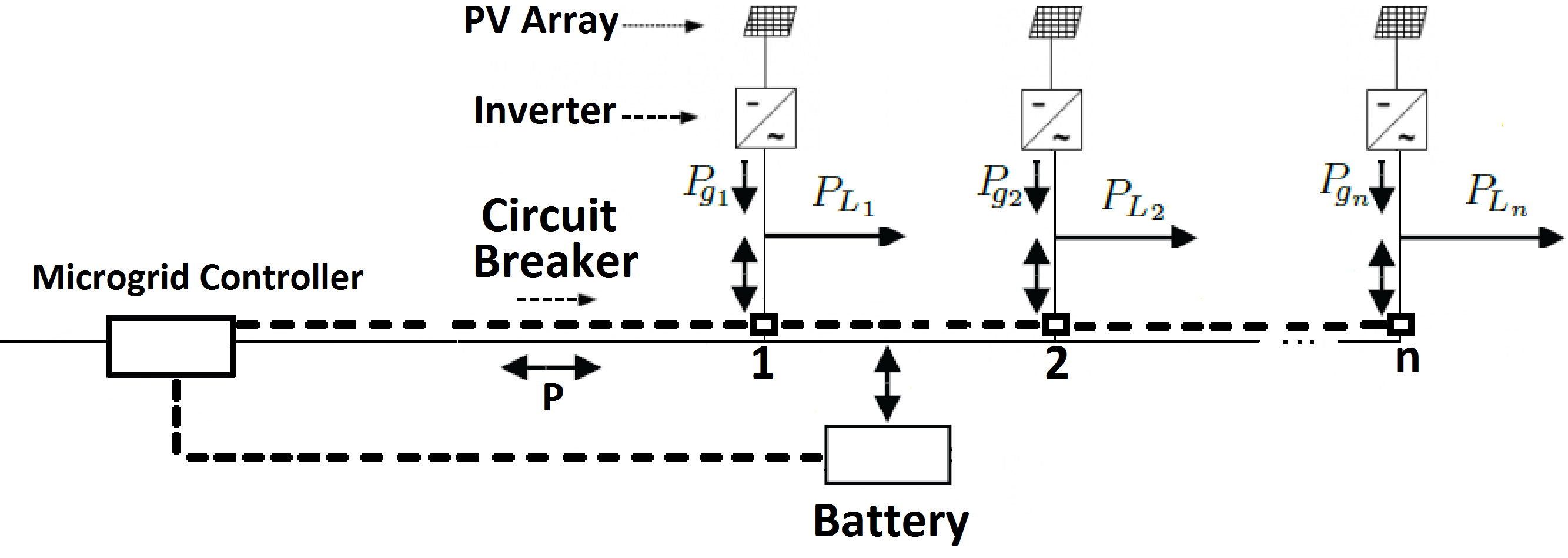
We consider a microgrid with local renewable energy resources (e.g. solar PV systems) and an energy storage unit as shown in Figure 1. Let $P_{L_{k}}$ and $P_{g_{k}}$ denote respectively the load and output of solar PV system of the $k$th consumer. The microgrid controller allows the distributed renewable generators to provide necessary active power locally or to the main grid. In addition, it directs load shedding and RE curtailment to obey a constraint on the max total active power that the microgrid can draw from, or inject into, the transmission line that connects it to the main grid. To this end, it uses the energy storage unit to minimize the curtailment of renewable energies and to minimize the load shedding. Intuitively, the energy storage unit can act as an energy reserve. However optimizing the usage of energy storage to minimize the risk of high amounts of load shedding and RE curtailment is a difficult and open problem.

Figure 1: Microgrid model: The dashed lines are the control signals and the solid lines are the power flow lines. The microgrid controller directs load shedding and RE curtailment using circuit breakers to maintain transmission line constraint.

The following notations are used in this work:

Notation:

• $d_{t}$ and $r_{t}$ are the load and renewable resource realizations respectively at time $t$.

• $\tilde{d}_{t}$ and $\tilde{r}_{t}$ are the load shedding and renewable resource curtailment respectively at time $t$.

• $|.|$ denotes the absolute value.

• $(.)^{+}=\max(.,0)$.

Electricity generated by renewable resources would first supply the local load. Any additional power needed to satisfy the load could be supplied from the grid or satisfied by discharging the battery. The energy in excess of the load, that is generated by renewable resources, can be used to charge the battery or be injected into the grid. The microgrid controller has the authority to curtail the excess RE injected into the grid and to direct the load to be shutdown. The total power to or from the microgrid must be less than a specific value that is specified by the main grid to satisfy, e.g, the transmission line constraints.

II-A Load and Renewable Energy

Let $\mathfrak{T}=\{1,2,...,T\}$ be the index set. Define $d=\{d_{t},t\in\mathfrak{T}\}$ and $r=\{r_{t},t\in\mathfrak{T}\}$ as random processes on the probability space $(\Omega,\mathfrak{F},\mathbb{P})$. $d$ and $r$ represent the load and renewable resource power respectively. For a fixed $t$, and for $\omega\in\Omega$, $d_{t}(\omega)$ and $r_{t}(\omega)$ are non-negative random variables with known continuous probability density functions. For the given $\omega\in\Omega$, $d_{t}$, and $r_{t}$ are deterministic functions of $t$ that denote the load realization and renewable resource power realization respectively at time $t$. Let $P_{L_{k}}^{t}$ and $P_{g_{k}}^{t}$ be respectively the load and output of solar PV system of the $k$th consumer in Figure 1 at time $t$. $d_{t}$ and $r_{t}$ are the aggregate consumers’ load and renewable power realization respectively,

$$d_{t}=P_{L_{1}}^{t}+P_{L_{2}}^{t}+...+P_{L_{n}}^{t},$$ (1)

$$r_{t}=P_{g_{1}}^{t}+P_{g_{2}}^{t}+...+P_{g_{n}}^{t}.$$

Below, the operating constraints for the energy storage are described.

II-B Energy Storage

Energy storage can charge or discharge $b_{t}$ amount of power at time $t$, $b_{t}$ can be either positive (battery is charging) or negative (battery is discharging). Let $s_{t}\geq 0$ denote the energy level of the battery at the beginning of the time $t$ for all $t=1,...,T$. State of charge of the battery, $s_{t}$, evolves according to

$$s_{t}=a\,\ s_{t-1}+b_{t-1}\,\ \Delta t$$ (2)

where $s_{t-1}$ is the energy level of the battery at the beginning of the time $t-1$, that is reduced by the factor $0<a<1$ at time $t$. It is assumed that $b_{t}$ is constant in the time slot $[t,t+\Delta t)$. The energy level of the battery is bounded by a minimum and maximum capacity

$$s^{\min}\leq s_{t}\leq s^{\max}.$$ (3)

Using (2), inequality (3) can be written as follows

$$\frac{s^{\min}-as_{t}}{\Delta t}\leq b_{t}\leq\frac{s^{\max}-as_{t}}{\Delta t}.$$ (4)

Maintaining constraints (2) and (4) is crucial in optimization of energy storage operations. The method by which the microgrid controller decides on the value of renewable energy curtailment and load shedding to maintain the transmission line constraint is described below.

II-C Renewable Energy Curtailment and Load Shedding

Renewable resources can be used to meet the load or charge the battery locally. The energy in excess of the load that is generated from the renewable resources can be injected into the grid. The microgrid controller can prohibit renewable resources from injecting energy into the grid, a process that is called resource curtailment. The resource curtailment, $\tilde{r}_{t}$, is bounded by

$$0\leq\tilde{r}_{t}\leq(r_{t}-b_{t}-d_{t})^{+}.$$ (5)

The load can be satisfied by using renewable resources or discharging the battery locally, and the extra energy needed to meet the load can be supplied from the grid. To prevent the violation of the transmission line constraint, excessive load can be avoided in a process known as load shedding. The load shedding, $\tilde{d}_{t}$, is bounded by

$$0\leq\tilde{d}_{t}\leq(d_{t}+b_{t}-r_{t})^{+}.$$ (6)

The power flow on the transmission line can be written as

$$p_{t}=d_{t}-\tilde{d}_{t}+b_{t}-r_{t}+\tilde{r}_{t}.$$ (7)

The grid controller provides $P^{\text{min}}$ and $P^{\text{max}}$ to the microgrid controller as the lower and upper bounds on the power flow $p_{t}$

$$P^{\text{min}}\leq p_{t}\leq P^{\text{max}}.$$ (8)

The main grid operator controls the output power of the generator, and provides the microgrid operator with a maximum net load. The microgrid operator controls the load shedding, $\tilde{d}_{t}$, and resource curtailment, $\tilde{r}_{t}$. The main grid controller’s objective is to control the power flow to avoid violation of the operating constraints (5)-(8). Let $n_{t}=d_{t}-r_{t}$ and $\tilde{n}_{t}=\tilde{d}_{t}-\tilde{r}_{t}$. Inequalities (5) and (6) can be written as

$$-(-n_{t}-b_{t})^{+}\leq\tilde{n}_{t}\leq(n_{t}+b_{t})^{+}.$$ (9)

Equation (7) can be written as

$$p_{t}=n_{t}-\tilde{n}_{t}+b_{t}.$$ (10)

The microgrid controller decides on the value of $\tilde{n}_{t}$, which is given as a function of $b_{t}$ as follows

$$\tilde{n}_{t}^{*}(b_{t})=\left\{\begin{array}[]{rcl}n_{t}+b_{t}-P^{\max}&\mbox{if}&(n_{t}+b_{t})>P^{\max}\\ n_{t}+b_{t}-P^{\min}&\mbox{if}&(n_{t}+b_{t})<P^{\min}\\ 0&\mbox{otherwise}&.\end{array}\right.$$ (14)

Let $\tilde{\mathfrak{n}}_{t}(b_{t})=\mid\tilde{n}_{t}^{*}(b_{t})\mid$. We use the abbreviation $\tilde{\mathfrak{n}}_{t}$ instead of $\tilde{\mathfrak{n}}_{t}(b_{t})$. Let $F_{\tilde{\mathfrak{n}}_{t}}$ be the cumulative distribution function for $\tilde{\mathfrak{n}}_{t}$. Below, the objective function of energy storage is defined in order to decrease the risk of high amounts of load shedding and RE curtailment.

II-D Risk Minimization

To define the objective function of the energy storage, we use the notion of Value-at-Risk (VaR) and Conditional Value-at-Risk (CVaR) [17]. $VaR_{\alpha}(\tilde{\mathfrak{n}}_{t})$ determines the worst possible $\tilde{\mathfrak{n}}_{t}$ that may occur with confidence level $\alpha$. For a given $0<\alpha<1$, the amount of load shedding and RE curtailment will not exceed $VaR_{\alpha}(\tilde{\mathfrak{n}}_{t})$ with probability $\alpha$,

$$VaR_{\alpha}(\tilde{\mathfrak{n}}_{t})=\min\{z|F_{\tilde{\mathfrak{n}}_{t}}(z)\geq\alpha\}.$$ (15)

$VaR_{\alpha}(\tilde{\mathfrak{n}}_{t})$ is a measure of risk, however it is not a reliable measure if $\tilde{\mathfrak{n}}_{t}$ has a fat tail distribution. $VaR_{\alpha}(\tilde{\mathfrak{n}}_{t})$ provides no information about the amount of $\tilde{\mathfrak{n}}_{t}$ that may occur beyond the value indicated by this measure [18]. CVaR is defined as the conditional expectation of load shedding and RE curtailment above the amount VaR_α. Let $E$ denote the expectation over $n_{t}$.

$$CVaR_{\alpha}(\tilde{\mathfrak{n}}_{t})=E[\tilde{\mathfrak{n}}_{t}|\tilde{\mathfrak{n}}_{t}>VaR_{\alpha}(\tilde{\mathfrak{n}}_{t})],$$ (16)

$$CVaR_{\alpha}(\tilde{\mathfrak{n}}_{t})=\int_{-\infty}^{\infty}zdF_{\tilde{\mathfrak{n}}_{t}}^{\alpha}(z),$$ (17)

where

$$F_{\tilde{\mathfrak{n}}_{t}}^{\alpha}(z)=\begin{cases}0,&\text{if }z<VaR_{\alpha}(\tilde{\mathfrak{n}}_{t})\\ \frac{F_{\tilde{\mathfrak{n}_{t}}}(z)-\alpha}{1-\alpha},&\text{otherwise}\end{cases}.$$

$CVaR_{\alpha}(\tilde{\mathfrak{n}}_{t})$ quantifies the value of the tail distribution of $\tilde{\mathfrak{n}}_{t}$ beyond the value of $VaR_{\alpha}(\tilde{\mathfrak{n}}_{t})$. $CVaR$ is a more conservative measure of risk than $VaR$, which is a lower bound on the risk. The function $g_{t}$ is defined as

$$g_{t}(b_{t})=CVaR_{\alpha}(\tilde{\mathfrak{n}}_{t}),$$ (18)

for every $t\in\{1,...,T\}$. At each given time $t$, the energy storage unit minimizes its own objective function on $b_{t},...,b_{T}$ as follows

$$\underset{w.r.t.\,\ (\ref{eq:one}),(\ref{eq:constraint})}{\min\limits_{b_{t},...,b_{T}}}\,\ \sum_{\tau=t}^{T}g_{\tau}(b_{\tau}).$$ (19)

Let $f_{t}$ be the density function of $n_{t}$. We assume the density function of ${n}_{t}$ satisfies Assumption $1$.

Assumption $1$: $f_{t}$ is strictly positive on the interval $[P^{\min}\,\ P^{\max}]$.

In the next section, it is proven that if Assumption $1$ holds, then the optimal decision for the energy storage with objective function (18) and (19) is unique for every $t\in\{1,...,T\}$.

III DYNAMIC PROGRAMMING FORMULATION

In this section, the optimization problem in (19) is reformulated as a dynamic programming problem. Let $J_{t}$ be the optimal objective function for the $(T-t)$-stage problem that starts at state $s_{t}$ at time $t$, and ends at time $T$,

$$J_{t}(s_{t})=\underset{w.r.t.\,\ (\ref{eq:one}),(\ref{eq:constraint})}{\min_{b_{t},...,b_{T}}}\sum_{\tau=t}^{T}g_{\tau}(b_{\tau}).$$ (20)

By applying the Dynamic Programming (DP),

$$J_{T+1}(s_{T+1})=0,$$

$$J_{t}(s_{t})=\underset{w.r.t.\,\ (\ref{eq:one}),(\ref{eq:constraint})}{\min_{b_{t}}}\{g_{t}(b_{t})+J_{t+1}(s_{t+1})\}.$$ (21)

By introducing the function $G_{t}$ for the given $s_{t}$

$$G_{t}(b_{t}|s_{t})=g_{t}(b_{t})+J_{t+1}(as_{t}+b_{t}\Delta t),$$ (22)

the DP equation (III) can be written as

$$J_{t}(s_{t})=\min_{w.r.t\,\ (\ref{eq:one}),(\ref{eq:constraint})}G_{t}(b_{t}|s_{t}),$$ (23)

where

$$s_{1}:=\arg\min_{s^{\min}\leq s_{1}\leq s^{\max}}J_{1}(s_{1}).$$ (24)

While the convexity of $CVaR_{\alpha}(\tilde{\mathfrak{n}}_{t})$ in $\tilde{\mathfrak{n}}_{t}$ is known [18], in the following Proposition we prove the strict convexity of $CVaR_{\alpha}(\tilde{\mathfrak{n}}_{t}(b_{t}))$ in $b_{t}$ if Assumption $1$ holds.

Proposition $1$: Let Assumption $1$ hold. Then, $g_{t}(b_{t})$ is strictly convex in $b_{t}$ for all $t=1,...,T$.

Proof:

The proof is given in Appendix A.∎

The constraints in minimization (23) interconnect the minimization of the first and second term in (22). In the following Theorems, it is shown that (23) is a convex optimization problem and therefore can be solved efficiently, e.g. by interior point methods [19].

Theorem $1$: Let Assumption $1$ hold. Then $G_{t}(b_{t}|s_{t})$ is convex in $(b_{t},s_{t})$ for the given $s^{\min}\leq s_{t}\leq s^{\max}$, and for all $b_{t}$ that satisfies (4).

Proof:

$J_{T+1}$ is the zero function and because of the convexity of $g_{T}(b_{T})$ in $b_{T}$ (Proposition $1$), $G_{T}(b_{T}|s_{T})$ is convex in $(b_{T},s_{T})$. Assume that $G_{t}(b_{t}|s_{t})$ is convex in $(b_{t},s_{t})$, the convexity of $G_{t-1}(b_{t-1}|s_{t-1})$ in $(b_{t-1},s_{t-1})$ is shown below. Let

$$G_{t-1}(b_{t-1}|s_{t-1})=g_{t-1}(b_{t-1})+J_{t}(s_{t}).$$ (25)

In Theorem $2$, it is proven that $J_{t}(s_{t})$ is convex in $s_{t}$ if $G_{t}(b_{t}|s_{t})$ is convex in $(b_{t},s_{t})$. Therefore from (25) and Proposition $1$, $G_{t-1}(b_{t-1}|s_{t-1})$ is convex in $(b_{t-1},s_{t-1})$. ∎

Theorem $2$: Let $s^{\min}\leq s_{t}\leq s^{\max}$ and $b_{t}$ satisfies inequality (4). If $G_{t}(b_{t}|s_{t})$ is convex in $(b_{t},s_{t})$ then $J_{t}(s_{t})$ is convex in $s_{t}$.

Proof:

The proof is given in Appendix B. ∎

The following Corollary implies the uniqueness of the optimal decision for the energy storage.

Corollary $1$: If Assumption $1$ holds, then for the given $s^{\min}\leq s_{t}\leq s^{\max}$, $G_{t}(b_{t}|s_{t})$ is strictly convex in $b_{t}$ for all $b_{t}$ that satisfies (4).

Proof:

From Proposition $1$, $g_{t}(b_{t})$ is strictly convex in $b_{t}$ and from Theorem $1$ and Theorem $2$, $J_{t+1}(s_{t+1})$ is convex in $s_{t+1}$. By induction and (22), it can be concluded that $G_{t}(b_{t}|s_{t})$ is strictly convex in $b_{t}$ for all $t=1,...,T$. ∎

The proofs of Theorem  $1$, Theorem $2$, and Corollary $1$ hold if we incorporate energy loss during the charging/discharging process of energy storage for a more realistic model. For example, the actual change of state of charge is $\eta_{in}b_{t}\Delta t$ when $b_{t}>0$, and $\frac{1}{\eta_{out}}b_{t}\Delta t$ when $b_{t}<0$, where $0<\eta_{in},\eta_{out}<1$ are the efficiency factors. Several distributions (e.g. Weibull, normal, Erlang, and beta) have been used to model the variations in the electric load [20]-[21]. Regardless of the type of distribution, the theoretical result of this work remains valid as long as the density function of $n_{t}$ satisfies Assumption $1$. Additionally, the proofs of Theorem $1$, Theorem $2$, and Corollary $1$ remain valid if the stage cost function, $g_{t}(b_{t})$, is any strict convex function in the charging/discharging rate of the battery. We use a normal distribution model for the $n_{t}$ in the following section for illustration.

IV SIMULATIONS

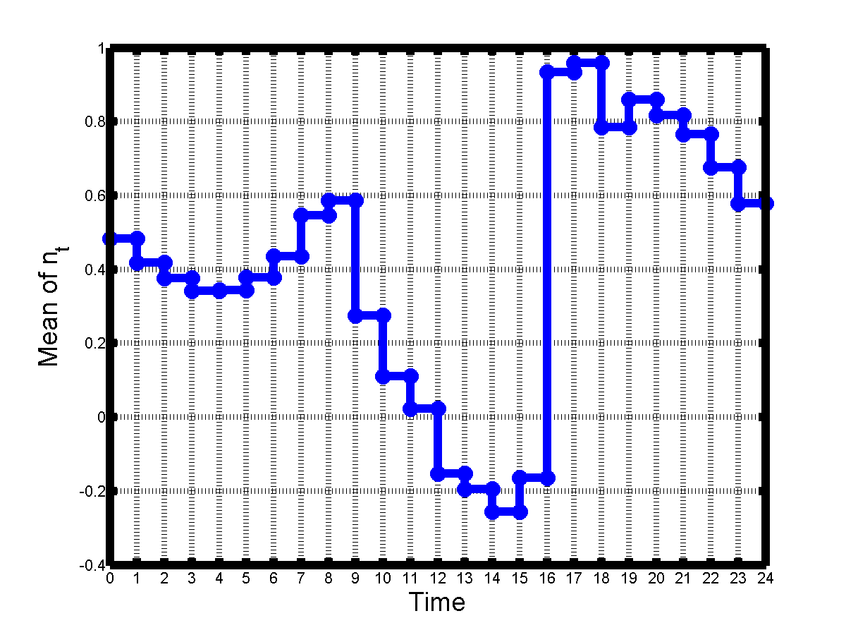
Example: We consider a $24$-stage storage optimization problem with given normalized parameters: $P^{\max}=0.6$, $P^{\min}=0$, $s^{\max}=1$, $s^{\min}=0$, $\alpha=0.01$ and $\Delta t=1$ hour. The random variable $n_{t}$ for all $t=0,...,23$ has a gaussian distribution. The mean of $n_{t}$ for all $t=0,...,23$ is plotted in the Figure 2. The standard deviation of $n_{t}$ is $0.25$.

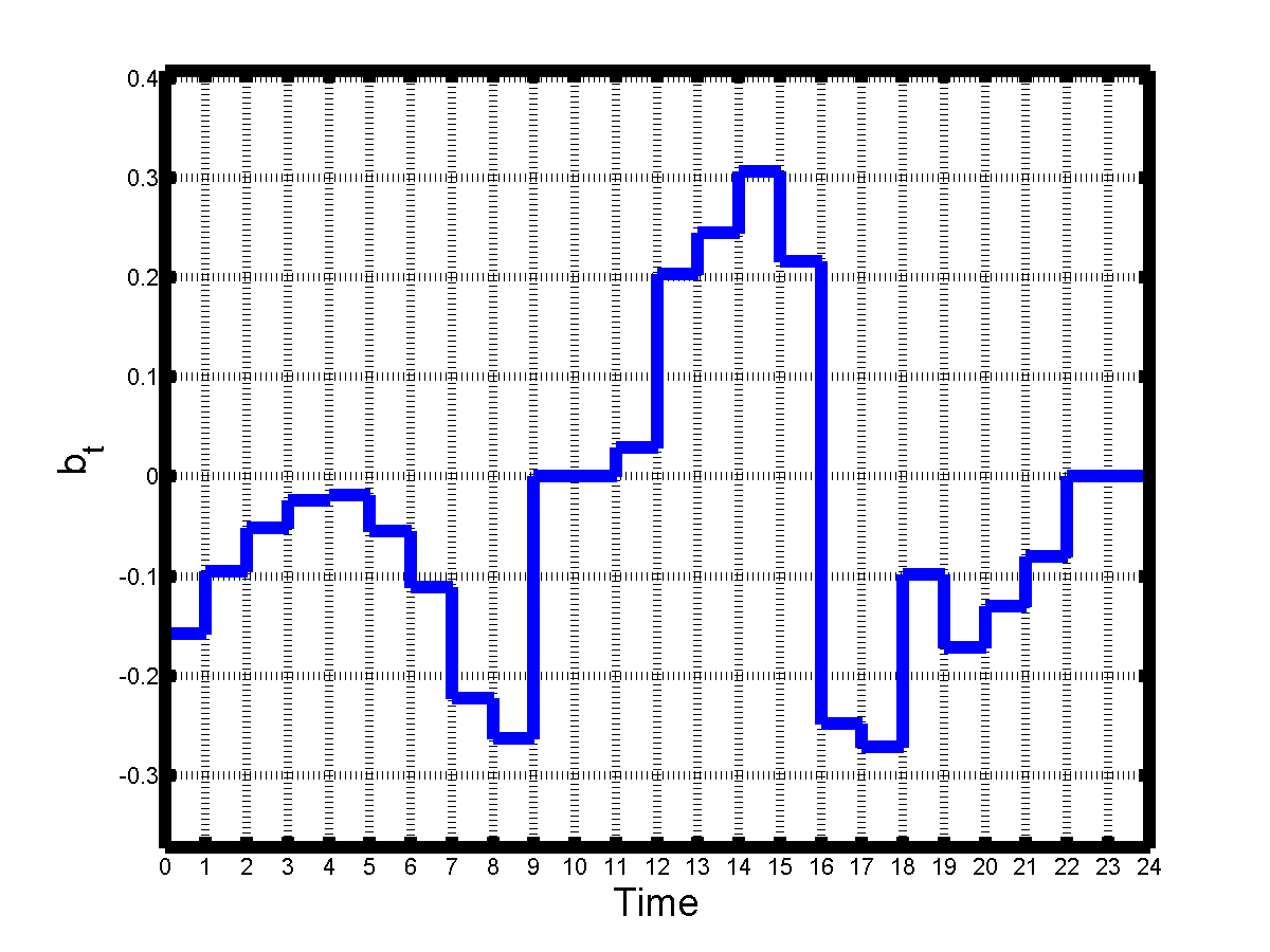
For the sake of simplicity, the presented simulations are limited to $24$ hours. However, in practice the analysis should be over the lifetime of the energy storage. We consider a realization of $n_{t}$, that is equal to the mean of the random variable $n_{t}$ as plotted in Figure 2. The charge and discharge rate of the energy storage is plotted in Figure 3. The energy level of the battery is plotted in Figure 4.

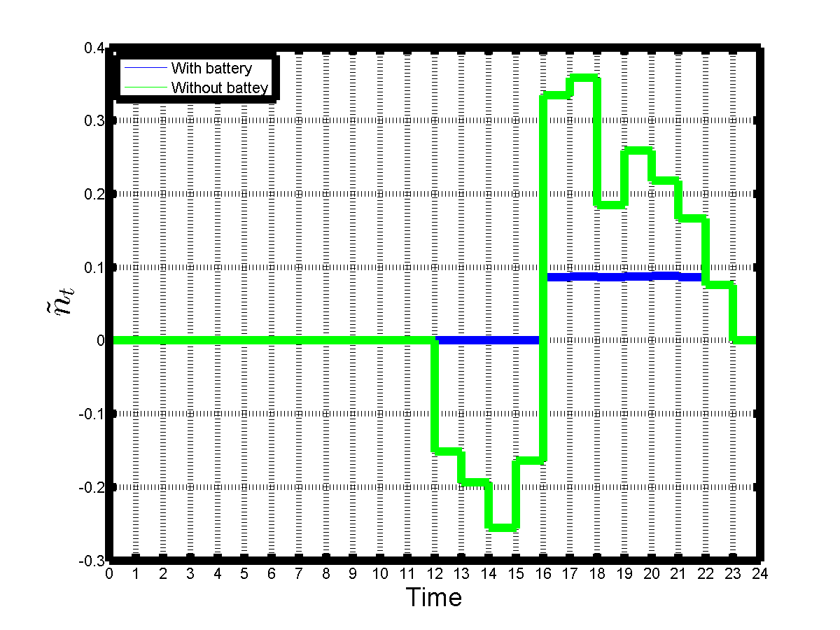
It is observed from Figures 3 and 4 that the battery is charged during the daytime with excess renewable energy generation and discharged during the morning and evening peak times. The load shedding and renewable energy curtailment for both scenarios, with battery (blue) and without battery (green), are plotted in Figure 5. It is observed that the energy storage with an optimal strategy, decreases renewable energy curtailment and load shedding significantly.

Figure 2: Mean of $n_{t}$.

Figure 3: The charge and discharge rate of energy storage.

Figure 4: State of charge of battery, $s_{t}$.

Figure 5: Load shedding (positive value) and renewable energy curtailment (negative value) with battery (blue) and without battery (green).

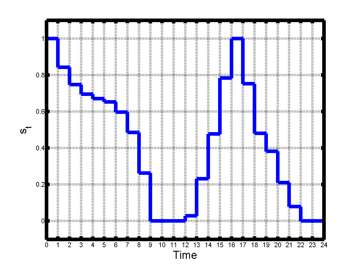
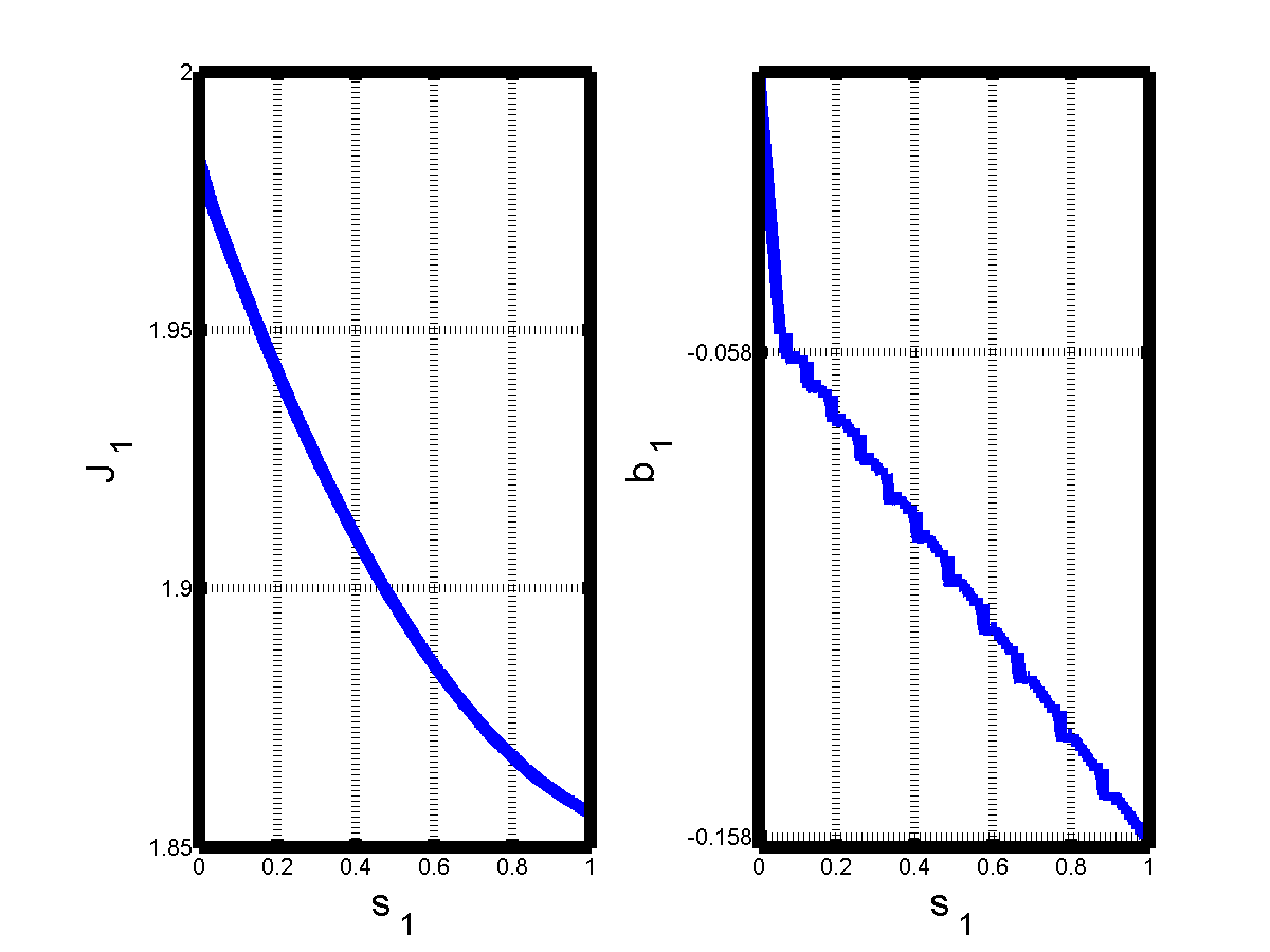
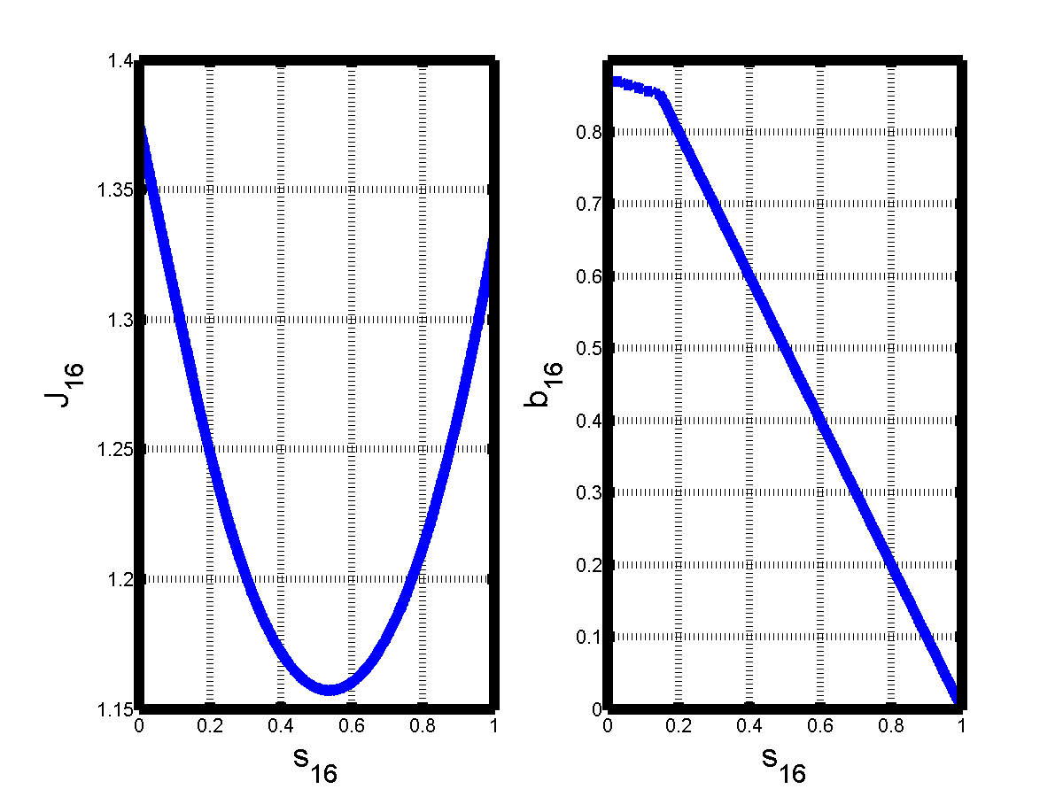
In Figures 6-7, the optimal objective function and charge/discharge rate is plotted as a function of the energy level of the energy storage for the time slots $12:00$ A.M.$-1:00$ A.M. and $3:00$ P.M.$-4:00$ P.M. The battery is charged from $3:00$ P.M. to $4:00$ P.M. and discharged from $12:00$ A.M. to $1:00$ A.M. It is observed that the optimal objective function $J_{t}(s_{t})$ is convex in the state of charge of the battery $s_{t}$. It is observed from Figure 6 that the optimal energy level for the battery is $1.00$, which is assumed to be the initial energy level of the battery in the Figure 4.

Figure 6: The optimal objective function and charge/discharge rate from 12:00 A.M. to 1:00 A.M.

Figure 7: The optimal objective function and charge/discharge rate from 3:00 P.M. to 4:00 P.M.

V CONCLUSIONS

In this work, a microgrid with renewable energy resources and an energy storage unit is considered. It is assumed that the load and RE are random processes over a finite time horizon. The main grid provides the microgrid operator with a total net load trajectory in order to satisfy the grid constraints. The net load trajectory is satisfied by the microgrid controller by applying renewable energy curtailment and load shedding. The energy storage unit is controlled by the microgrid independently from the main grid controller. The microgrid controller decides on charging and discharging strategies in order to minimize the risk of high amounts of load shedding and RE curtailment within a finite time horizon. The energy storage objective function in the grid is formulated as a finite stage dynamic programming problem. It is proven that under sufficient conditions the multi-stage objective function of energy storage is strictly convex in the charging/discharging rate. Thus, the optimal decision at each stage is unique for the given state of charge of the battery. The convexity of the objective function in charge/discharge rate, is needed for implementing mathematical programming that searches within the action space. Finally, numerical results are presented for an energy storage unit with a multistage objective function in a microgrid with random load and RE. It is observed that an optimal charging/discharching strategy for the energy storage based on an stochastic model for the load and renewable generation, can decrease the realized RE curtailment and load shedding.

APPENDIX

V-A Proof of Proposition $1$

Proof:

Let $f_{t}$ be the density function of $n_{t}$. Without loss of generality assume $\alpha=0$, from (15)-(18)

$$g_{t}(b_{t})= \int_{P^{\max}-b_{t}}^{\infty}(n_{t}+b_{t}-P^{\max})f_{t}\partial n_{t}$$ (26)

$$-\int_{-\infty}^{P^{\min}-b_{t}}(n_{t}+b_{t}-P^{\min})f_{t}\partial n_{t}.$$

Below, it is shown that $\int_{P^{\max}-b_{t}}^{\infty}(n_{t}+b_{t}-P^{\max})f_{t}\partial n_{t}$ is strictly convex in $b_{t}$. Without loss of generality, assume $x<\gamma x+(1-\gamma)y<y$. Below it is shown that for all $\gamma\in(0,1)$ and $x\neq y$

$$\int_{P^{\max}-\gamma x-(1-\gamma)y}^{\infty}\big{(}n_{t}+\gamma x+(1-\gamma)y-P^{\max}\big{)}f_{t}\partial n_{t}$$ (27)

$$\,\ \,\ \,\ \,\ \,\ \,\ \,\ \,\ \,\ \,\ \,\ \,\ \,\ \,\ \,\ <$$

$$\gamma\int_{P^{\max}-x}^{\infty}(n_{t}+x-P^{\max})f_{t}\partial n_{t}$$

$$+(1-\gamma)\int_{P^{\max}-y}^{\infty}(n_{t}+y-P^{\max})f_{t}\partial n_{t}.$$

The right hand side of inequality (27) is equal to

$$\gamma\int_{P^{\max}-\gamma x-(1-\gamma)y}^{\infty}(n_{t}+x-P^{\max})f_{t}\partial n_{t}$$ (28)

$$-\gamma\int_{P^{\max}-\gamma x-(1-\gamma)y}^{P^{\max}-x}(n_{t}+x-P^{\max})f_{t}\partial n_{t}$$

$$+(1-\gamma)\int_{P^{\max}-y}^{P^{\max}-\gamma x-(1-\gamma)y}(n_{t}+y-P^{\max})f_{t}\partial n_{t}$$

$$+(1-\gamma)\int_{P^{\max}-\gamma x-(1-\gamma)y}^{\infty}(n_{t}+y-P^{\max})f_{t}\partial n_{t}$$

$$=\int_{P^{\max}-\gamma x-(1-\gamma)y}^{\infty}\big{(}n_{t}+\gamma x+(1-\gamma)y-P^{\max}\big{)}f_{t}\partial n_{t}$$

$$-\gamma\int_{P^{\max}-\gamma x-(1-\gamma)y}^{P^{\max}-x}(n_{t}+x-P^{\max})f_{t}\partial n_{t}$$

$$+(1-\gamma)\int_{P^{\max}-y}^{P^{\max}-\gamma x-(1-\gamma)y}(n_{t}+y-P^{\max})f_{t}\partial n_{t}.$$

The strict convexity follows from Assumption $1$, and

$$\int_{P^{\max}-\gamma x-(1-\gamma)y}^{P^{\max}-x}(n_{t}+x-P^{\max})f_{t}\partial n_{t}<0$$

and

$$\int_{P^{\max}-y}^{P^{\max}-\gamma x-(1-\gamma)y}(n_{t}+y-P^{\max})f_{t}\partial n_{t}>0.$$

Similarly, it can be shown that $-\int_{-\infty}^{P^{\min}-b_{t}}(n_{t}+b_{t}-P^{\min})f_{t}\partial n_{t}$ is strictly convex in $b_{t}$. Therefore, $g_{t}(b_{t})$ is strictly convex in $b_{t}$. ∎

V-B Proof of Theorem $2$

Proof:

Without loss of generality, assume

$$s^{\min}\leq x<\alpha x+(1-\alpha)\acute{x}<\acute{x}\leq s^{\max},$$ (29)

It is shown below that for all $\alpha\in(0,1)$, and $x$ and $\acute{x}$ that satisfy (29)

$$J_{t}\big{(}\alpha x+(1-\alpha)\acute{x}\big{)}\leq\alpha J_{t}(x) +(1-\alpha)J_{t}(\acute{x}).$$ (30)

Suppose, there exists an $x$ and $\acute{x}$, $s^{\min}\leq x<\acute{x}\leq s^{\max}$, and $\alpha\in(0,1)$ such that

$$J_{t}\big{(}\alpha x+(1-\alpha)\acute{x}\big{)}>\alpha J_{t}(x)+(1-\alpha)J_{t}(\acute{x}).$$ (31)

Let

$$b_{t}^{m}(x)={\arg{\min_{{\frac{s^{\text{min}}-ax}{\Delta t}\leq b_{t}\leq\frac{s^{\text{max}}-ax}{\Delta t}}}}G_{t}(b_{t}|x)},$$ (32)

$$\bar{x}=\alpha x+(1-\alpha)\acute{x}.$$

It can be proven by induction that $G_{t}(b_{t}|x)$ is continuous in $b_{t}$ for all $t=1,...,T$. Because of the compactness of the domain in (32) and the continuity of $G_{t}(b_{t}|x)$ in $b_{t}$ the minimizer exists. From (23), (31), and (32), it can be concluded that

$$G_{t}(b_{t}^{m}(\bar{x})|\bar{x})>\alpha G_{t}(b_{t}^{m}(x)|x)+(1-\alpha)G_{t}(b_{t}^{m}(\acute{x})|\acute{x}).$$ (33)

It is evident that

$$\frac{s^{\text{min}}-\bar{x}}{\Delta t}\geq\alpha b_{t}^{m}(x)+(1-\alpha)b_{t}^{m}(\acute{x})\geq\frac{s^{\text{max}}-\bar{x}}{\Delta t}.$$ (34)

From (32), (33), and (34), it can be concluded that

$$G_{t}(\alpha b_{t}^{m}(x)+(1-\alpha)b_{t}^{m}(\acute{x})|\bar{x})$$ (35)

$$\geq G_{t}(b_{t}^{m}(\bar{x})|\bar{x})$$

$$>\alpha G_{t}(b_{t}^{m}(x)|x)+(1-\alpha)G_{t}(b_{t}^{m}(\acute{x})|\acute{x}).$$

The first inequality is because of (34), and $b_{t}^{m}(\bar{x})$ being the minimizer of $G_{t}(.|\bar{x})$. The second inequality is because of (33). Inequality (35) contradicts the convexity of $G_{t}(b_{t}|s_{t})$ in $(b_{t},s_{t})$, therefore $J_{t}(s_{t})$ is convex for $s^{\max}\leq s_{t}\leq s^{\min}$. ∎

References

- [1] A. Zeinalzadeh, and Vijay Gupta, Pricing energy in the presence of renewables, Submitted to the IEEE Power and Energy Society General Meeting 2017.
- [2] A. Zeinalzadeh, R. Ghorbani, E. Reihani, Optimal power flow problem with energy storage voltage and reactive power control, The 45th ISCIE International Symposium on Stochastic Systems Theory and Its Applications, Okinawa, Nov. 2013.
- [3] A. Zeinalzadeh, R. Ghorbani, J. Yee, Stochastic model of voltage variations in the presence of photovoltaic systems, IEEE American Control Conference (ACC), Boston, MA, USA, July 6-8, 2016.
- [4] Grid integration of large-capacity Renewable Energy sources and use of large-capacity Electrical Energy Storage, Technical report, International Electrotechnical Commision (IEC), OCT 2012.
- [5] R. Golden and B. Paulos, Curtailment of renewable energy in california and beyond, The Electricity Journal, Vol. 28, Issue 6, 2015.
- [6] A. Outdalov, D. Chatouni, and C. Ohler. Optimizing a battery energy storage system for primary frequency control. IEEE Transactions on Power Systems, 22 (3), pp. 1259–1266, 2007.
- [7] P. Mercier, R. Cherkaoui, and A Oudalov, Optimizing a battery energy storage system for frequency control application in an isolated power system. IEEE Transactions on Power Systems, 24(3), pp. 1469–1477, 2009.
- [8] Yashodhan Kanoria, Andrea Montanari, David Tse, Baosen Zhang, Distributed storage for intermittent energy sources: control design and performance limits, working paper.
- [9] Kyri Baker, Gabriela Hug, and Xin Li, Optimal integration of intermittent energy sources using distributed multi-step optimization, Power and Energy Society General Meeting, pp. 1–8, 2012.
- [10] Kai Wang, Chuang Lin and Steven Low, How stochastic network calculus concepts help green the power grid, Proceedings of IEEE SmartGridComm Conference, 2011.
- [11] Huan Xu, Ufuk Topcu, Steven Low, Christopher Clarke and K. Mani Chandy, Load-shedding probabilities with hybrid renewable power generation and energy storage, Proceedings of Allerton, 2010.
- [12] A. Even, J. Neyens, and A Demouselle, Peak shaving with batteries. In the Proceedings of 12th International Conference on Electricity Distribution, vol. 5, 1993.
- [13] Kottick, M. Blau, Operational and economic benefits of battery energy storage plants, International Journal of Electrical Power and Energy Systems, 15(6), pp. 345–349, 1993.
- [14] K. Mani Chandy, Steven H. Low, Ufuk Topcu and Huan Xu. A Simple optimal power flow model with energy storage, IEEE CDC 2010, pp. 1051–1057.
- [15] P. Anderson and M. Mirheydar, An adaptive method for setting underfrequency load shedding relays, IEEE Trans. Power Syst., vol. 7, no. 2, pp. 647–655, 1992.
- [16] X. Lou, D. K. Y. Yau, H. H. Nguyen, and B. Chen, Profit-Optimal and stability-aware load curtailment in smart grids, IEEE Transactions on Smart Grid, vol. 4, no. 3, 2013.
- [17] S. Uryasev, R. T. Rockafellar, Optimization of conditional value at risk. Research Report 99–4, ISE Dept. Univeristy of Florida, 1999.
- [18] R. T. Rockafellar, S. Uryasev, Conditional value-at-risk for general loss distributions, Journal of Banking and Finance, 26, pp. 1443–1471, 2002.
- [19] S. Boyd and L. Vandenberghe. Convex Optimization. Cambridge University Press, 2004.
- [20] Ravindra Singh, Bikash C. Pal, and Rabih A. Jabr, Statistical representation of distribution system loads using gaussian mixture model, IEEE Transactions on Power Systems, vol. 25, no. 1, 2010.
- [21] S. W. Heunis and R. Herman, A probabilistic model for residential consumer loads, IEEE Transaction on Power Systems, vol. 17, no. 3, pp. 621–625, 2002.