Abstract

The spiking activity of single neurons can be well described by a nonlinear integrate-and-fire model that includes somatic adaptation. When exposed to fluctuating inputs sparsely coupled populations of these model neurons exhibit stochastic collective dynamics that can be effectively characterized using the Fokker-Planck equation. This approach, however, leads to a model with an infinite-dimensional state space and non-standard boundary conditions. Here we derive from that description four simple models for the spike rate dynamics in terms of low-dimensional ordinary differential equations using two different reduction techniques: one uses the spectral decomposition of the Fokker-Planck operator, the other is based on a cascade of two linear filters and a nonlinearity, which are determined from the Fokker-Planck equation and semi-analytically approximated. We evaluate the reduced models for a wide range of biologically plausible input statistics and find that both approximation approaches lead to spike rate models that accurately reproduce the spiking behavior of the underlying adaptive integrate-and-fire population. Particularly the cascade-based models are overall most accurate and robust, especially in the sensitive region of rapidly changing input. For the mean-driven regime, when input fluctuations are not too strong and fast, however, the best performing model is based on the spectral decomposition. The low-dimensional models also well reproduce stable oscillatory spike rate dynamics that are generated either by recurrent synaptic excitation and neuronal adaptation or through delayed inhibitory synaptic feedback. The computational demands of the reduced models are very low but the implementation complexity differs between the different model variants. Therefore we have made available implementations that allow to numerically integrate the low-dimensional spike rate models as well as the Fokker-Planck partial differential equation in efficient ways for arbitrary model parametrizations as open source software. The derived spike rate descriptions retain a direct link to the properties of single neurons, allow for convenient mathematical analyses of network states, and are well suited for application in neural mass/mean-field based brain network models.

Author summary

Characterizing the dynamics of biophysically modeled, large neuronal networks usually involves extensive numerical simulations. As an alternative to this expensive procedure we propose efficient models that describe the network activity in terms of a few ordinary differential equations. These systems are simple to solve and allow for convenient investigations of asynchronous, oscillatory or chaotic network states because linear stability analyses and powerful related methods are readily applicable. We build upon two research lines on which substantial efforts have been exerted in the last two decades: (i) the development of single neuron models of reduced complexity that can accurately reproduce a large repertoire of observed neuronal behavior, and (ii) different approaches to approximate the Fokker-Planck equation that represents the collective dynamics of large neuronal networks. We combine these advances and extend recent approximation methods of the latter kind to obtain spike rate models that surprisingly well reproduce the macroscopic dynamics of the underlying neuronal network. At the same time the microscopic properties are retained through the single neuron model parameters. To enable a fast adoption we have released an efficient Python implementation as open source software under a free license.

Introduction

There is prominent evidence that information in the brain, about a particular stimulus for example, is contained in the collective neuronal spiking activity averaged over populations of neurons with similar properties (population spike rate code) [1, 2]. Although these populations can comprise a large number of neurons [3], they often exhibit low-dimensional collective spiking dynamics [4] that can be measured using neural mass signals such as the local field potential or electroencephalography.

The behavior of cortical networks at that level is often studied computationally by employing simulations of multiple (realistically large or subsampled) populations of synaptically coupled individual spiking model neurons. A popular choice of single cell description for this purpose are two-variable integrate-and-fire models [5, 6] which describe the evolution of the fast (somatic) membrane voltage and an adaptation variable that represents a slowly-decaying potassium current. These models are computationally efficient and can be successfully calibrated using electrophysiological recordings of real cortical neurons and standard stimulation protocols [5, 7, 8, 9, 10] to accurately reproduce their subthreshold and spiking activity. The choice of such (simple) neuron models, however, does not imply reasonable (short enough) simulation durations for a recurrent network, especially when large numbers of neurons and synaptic connections between them are considered.

A fast and mathematically tractable alternative to simulations of large networks are population activity models in terms of low-dimensional ordinary differential equations (i.e., which consist of only a few variables) that typically describe the evolution of the spike rate. These reduced models can be rapidly solved and allow for convenient analyses of the dynamical network states using well-known methods that are simple to implement. A popular example are the Wilson-Cowan equations [11], which were also extended to account for (slow) neuronal adaptation [12] and short-term synaptic depression [13]. Models of this type have been successfully applied to qualitatively characterize the possible dynamical states of coupled neuronal populations using phase space analyses [12, 13, 11], yet a direct link to more biophysically described networks of (calibrated) spiking neurons in terms of model parameters is missing.

Recently, derived population activity models have been proposed that bridge the gap between single neuron properties and mesoscopic network dynamics. These models are described by integral equations [14, 15] or partial differential equations [16, 17]

Here we derive simple models in terms of low-dimensional ordinary differential equations (ODEs) for the spike rate dynamics of sparsely coupled adaptive nonlinear integrate-and-fire neurons that are exposed to noisy synaptic input. The derivations are based on a Fokker-Planck equation that describes the neuronal population activity in the mean-field limit of large networks. We develop reduced models using recent methodological advances on two different approaches: the first is based on a spectral decomposition of the Fokker-Planck operator under two different slowness assumptions [18, 19, 20]. In the second approach we consider a cascade of linear temporal filters and a nonlinear function which are determined from the Fokker-Planck equation and semi-analytically approximated, building upon [21]. Both approaches are extended for an adaptation current, a nonlinear spike generating current and recurrent coupling with distributed synaptic delays.

We evaluate the developed low-dimensional spike rate models quantitatively in terms of reproduction accuracy in a systematic manner over a wide range of biologically plausible parameter values. In addition, we provide numerical implementations for the different reduction methods as well as the Fokker-Planck equation under a free license as open source project.

For the derived models in this contribution we use the adaptive exponential integrate-and-fire (aEIF) model [5] to describe individual neurons, which is similar to the model proposed by Izhikevich [6] but includes biophysically meaningful parameters and a refined description of spike initiation. However, the presented derivations are equally applicable when using the Izhikevich model instead (requiring only a small number of simple substitutions in the code).

Through their parameters the derived models retain a direct, quantitative link to the underlying spiking model neurons, and they are described in a well-established, convenient form (ODEs) that can be rapidly solved and analyzed. Therefore, these models are well suited (i) for mathematical analyses of dynamical states at the population level, e.g., linear stability analyses of attractors, and (ii) for application in multi-population brain network models. Apart from a specific network setting, the derived models are also appropriate as a spike rate description of individual neurons under noisy input conditions.

The structure of this article contains mildly redundant model specifications allowing the readers who are not interested in the methodological foundation to directly read the self-contained Sect. Results.

Results

Model reduction

The quantity of our interest is the population-averaged number of spikes emitted by a large homogeneous network of $N$ sparsely coupled aEIF model neurons per small time interval, i.e., the spike rate $r_{N}(t)$. The state of neuron $i$ at time $t$ is described by the membrane voltage $V_{i}(t)$ and adaptation current $w_{i}(t)$, which evolve piecewise continuously in response to overall synaptic current $I_{\mathrm{syn},i}=I_{\mathrm{ext},i}(t)+I_{\mathrm{rec},i}(t)$. This input current consists of fluctuating network-external drive $I_{\mathrm{ext},i}=C[\mu_{\mathrm{ext}}(t)+\sigma_{\mathrm{ext}}(t)\xi_{\mathrm{ext},i}(t)]$ with membrane capacitance $C$, time-varying moments $\mu_{\mathrm{ext}}$, $\sigma_{\mathrm{ext}}^{2}$ and unit Gaussian white noise process $\xi_{\mathrm{ext},i}$ as well as recurrent input $I_{\mathrm{rec,i}}$. The latter causes delayed postsynaptic potentials (i.e., deflections of $V_{i}$) of small amplitude $J$ triggered by the spikes of $K$ presynaptic neurons (see Sect. Methods for details).

Here we present two approaches of how the spike rate dynamics of the large, stochastic delay-differential equation system for the $2N$ states $(V_{i},w_{i})$ can be described by simple models in terms of low-dimensional ODEs. Both approaches (i) take into account adaptation current dynamics that are sufficiently slow, allowing to replace the individual adaptation current $w_{i}$ by its population-average $\langle w\rangle$, governed by

$$\frac{d{\langle w\rangle}}{dt}=\frac{a\left(\langle V\rangle_{\infty}-E_{w}\vphantom{{}^{2}}\right)-\langle w\rangle}{\tau_{w}}+b\,r(t),$$ (1)

where $a$, $E_{w}$, $b$, $\tau_{w}$ are the adaptation current model parameters (subthreshold conductance, reversal potential, spike-triggered increment, time constant, respectively), $\langle V\rangle_{\infty}$ is the steady-state membrane voltage averaged across the population (which can vary over time, see below), and $r$ is the spike rate of the respective low-dimensional model. Furthermore, both approaches (ii) are based on the observation that the collective dynamics of a large, sparsely coupled (and noise driven) network of integrate-and-fire type neurons can be well described by a Fokker-Planck equation. In this intermediate Fokker-Planck (FP) model the overall synaptic input is approximated by a mean part with additive white Gaussian fluctuations, $I_{\mathrm{syn,i}}/C\approx\mu_{\mathrm{syn}}(t,r_{d})+\sigma_{\mathrm{syn}}(t,r_{d})\xi_{i}(t)$, that are uncorrelated between neurons. The moments of the overall synaptic input,

$$\mu_{\mathrm{syn}}=\mu_{\mathrm{ext}}(t)+JKr_{d}(t),\qquad\sigma^{2}_{\mathrm{syn}}=\sigma_{\mathrm{ext}}^{2}(t)+J^{2}Kr_{d}(t),$$ (2)

depend on time via the moments of the external input and, due to recurrent coupling, on the delayed spike rate $r_{d}$. The latter is governed by

$$\frac{dr_{d}}{dt}=\frac{r-r_{d}}{\tau_{d}},$$ (3)

which corresponds to individual propagation delays drawn from an exponentially distributed random variable with mean $\tau_{d}$. The FP model involves solving a partial differential equation (PDE) to obtain the time-varying membrane voltage distribution $p(V,t)$ and the spike rate $r(t)$.

The first reduction approach is based on the spectral decomposition of the Fokker-Planck operator $\mathcal{L}$ and leads to the following two low-dimensional models: the “basic” model variant (spec₁) is given by a complex-valued differential equation describing the spike rate evolution in its real part,

$$\frac{d\tilde{r}}{dt}=\lambda_{1}(\tilde{r}-r_{\infty}),\qquad r(t)=\mathrm{Re}\{\tilde{r}\},$$ (4)

where $\lambda_{1}(\mu_{\mathrm{tot}},\sigma_{\mathrm{tot}})$ is the dominant eigenvalue of $\mathcal{L}$ and $r_{\infty}(\mu_{\mathrm{tot}},\sigma_{\mathrm{tot}})$ is the steady-state spike rate. Its parameters $\lambda_{1}$, $r_{\infty}$, and $\langle V\rangle_{\infty}$ (cf. Eq. (1)) depend on the total input moments given by $\mu_{\mathrm{tot}}(t)=\mu_{\mathrm{syn}}-\langle w\rangle/C$ and $\sigma_{\mathrm{tot}}^{2}(t)=\sigma_{\mathrm{syn}}^{2}$ which closes the model (Eqs. (1)–(4)). The other, “advanced” spectral model variant (spec₂) is given by a real-valued second order differential equation for the spike rate,

$$\beta_{2}\,\ddot{r}+\beta_{1}\,\dot{r}+\beta_{0}\,r=r_{\infty}-r-\beta_{c},$$ (5)

where the dots denote time derivatives. Its parameters $\beta_{2}$, $\beta_{1}$, $\beta_{0}$, $\beta_{c}$, $r_{\infty}$ and $\langle V\rangle_{\infty}$ depend on the total input moments $(\mu_{\mathrm{tot}},\sigma_{\mathrm{tot}}^{2})$ as follows: the latter two parameters explicitly as in the basic model above, the former four indirectly via the first two dominant eigenvalues $\lambda_{1}$, $\lambda_{2}$ and via additional quantities obtained from the (stationary and the first two nonstationary) eigenfunctions of $\mathcal{L}$ and its adjoint $\mathcal{L}^{*}$. Furthermore, the parameter $\beta_{c}$ depends explicitly on the population-averaged adaptation current $\langle w\rangle$, the delayed spike rate $r_{d}$, and on the first and second order time derivatives of the external moments $\mu_{\mathrm{ext}}$ and $\sigma^{2}_{\mathrm{ext}}$.

The second approach is based on a Linear-Nonlinear (LN) cascade, in which the population spike rate is generated by applying to the time-varying mean and standard deviation of the overall synaptic input, $\mu_{\mathrm{syn}}$ and $\sigma_{\mathrm{syn}}$, separately a linear temporal filter, followed by a common nonlinear function. These three components – two linear filters and a nonlinearity – are extracted from the Fokker-Planck equation. Approximating the linear filters using exponentials and damped oscillating functions yields two model variants: In the basic “exponential” (LN_exp) model the filtered mean $\mu_{\mathrm{f}}$ and standard deviation $\sigma_{\mathrm{f}}$ of the overall synaptic input are given by

$$\frac{d\mu_{\mathrm{f}}}{dt}=\frac{\mu_{\mathrm{syn}}-\mu_{\mathrm{f}}}{\tau_{\mu}},\qquad\frac{d\sigma_{\mathrm{f}}}{dt}=\frac{\sigma_{\mathrm{syn}}-\sigma_{\mathrm{f}}}{\tau_{\sigma}},$$ (6)

where the time constants $\tau_{\mu}(\mu_{\mathrm{eff}},\sigma_{\mathrm{eff}})$, $\tau_{\sigma}(\mu_{\mathrm{eff}},\sigma_{\mathrm{eff}})$ depend on the effective (filtered) input mean $\mu_{\mathrm{eff}}(t)=\mu_{\mathrm{f}}-\langle w\rangle/C$ and standard deviation $\sigma_{\mathrm{eff}}(t)=\sigma_{\mathrm{f}}$. The “damped oscillator” (LN_dos) model variant, on the other hand, describes the filtered input moments by

$$\ddot{\mu}_{\mathrm{f}}+\frac{2}{\tau}\dot{\mu}_{\mathrm{f}}+\left(\frac{2}{\tau^{2}}+\omega^{2}\right)\mu_{\mathrm{f}} =\frac{1+\tau^{2}\omega^{2}}{\tau}\left(\frac{\mu_{\mathrm{syn}}}{\tau}+\dot{\mu}_{\mathrm{syn}}\right),$$ (7)

$$\frac{d\sigma_{\mathrm{f}}}{dt} =\frac{\sigma_{\mathrm{syn}}-\sigma_{\mathrm{f}}}{\tau_{\sigma}},$$ (8)

where the time constants $\tau(\mu_{\mathrm{tot}},\sigma_{\mathrm{tot}})$, $\tau_{\sigma}(\mu_{\mathrm{tot}},\sigma_{\mathrm{tot}})$ and the angular frequency $\omega(\mu_{\mathrm{tot}},\sigma_{\mathrm{tot}})$ depend on the total input moments defined above. In both LN model variants the spike rate is obtained by the nonlinear transformation of the effective input moments through the steady-state spike rate,

$$r(t)=r_{\infty}\!\left(\mu_{\mathrm{eff}},\,\sigma_{\mathrm{eff}}\right),$$ (9)

and the steady-state mean membrane voltage $\langle V\rangle_{\infty}$ (cf. Eq. (1)) is also evaluated at $(\mu_{\mathrm{eff}},\sigma_{\mathrm{eff}})$.

These four models (spec₁, spec₂, LN_exp, LN_dos) from both reduction approaches involve a number of parameters that depend on the strengths of synaptic input and adaptation current only via the total or effective input moments. We refer to these parameters as quantities below to distinguish them from fixed (independent) parameters. The computational complexity when numerically solving the models forward in time (for different parametrizations) can be greatly reduced by precomputing those quantities for a range of values for the total/effective input moments and using look-up tables during time integration. Changing any parameter value of the external input, the recurrent coupling or the adaptation current does not require renewed precomputations, enabling rapid explorations of parameter space and efficient (linear) stability analyses of network states.

The full specification of the “ground truth” system (network of aEIF neurons), the derivations of the intermediate description (FP model) and the low-dimensional spike rate models complemented by concrete numerical implementations are provided in Sect. Methods (that is complemented by the supporting material S1 Text). In Fig. 1 we visualize the outputs of the different models using an example excitatory aEIF network exposed to external input with varying mean $\mu_{\mathrm{ext}}(t)$ and standard deviation $\sigma_{\mathrm{ext}}(t)$.

Performance for variations of the mean input

Here, and in the subsequent two sections, we assess the accuracy of the four low-dimensional models to reproduce the spike rate dynamics of the underlying aEIF population. The intermediate FP model is included for reference. The derived models generate population activity in response to overall synaptic input moments $\mu_{\mathrm{syn}}$ and $\sigma_{\mathrm{syn}}^{2}$. These depend on time via the external moments $\mu_{\mathrm{ext}}(t)$ and $\sigma_{\mathrm{ext}}^{2}(t)$, and the delayed spike rate $r_{d}(t)$. Therefore, it is instrumental to first consider an uncoupled population and suitable variations of external input moments that effectively mimic a range of biologically plausible presynaptic spike rate dynamics. This allows us to systematically compare the reproduction performance of the different models over a manageable parameter space (without $K$, $J$, $\tau_{d}$), yet it provides useful information on the accuracy for recurrent networks.

For many network settings the dominant effect of synaptic coupling is on the mean input (cf. Eq. (2)). Therefore, we consider first in detail time-varying mean but constant variance of the input. Specifically, to account for a wide range of oscillation frequencies for presynaptic spike rates, $\mu_{\mathrm{ext}}$ is described by an Ornstein-Uhlenbeck (OU) process

$$\dot{\mu}_{\mathrm{ext}}=\frac{\bar{\mu}-\mu_{\mathrm{ext}}}{\tau^{\mu}_{\mathrm{ou}}}+\sqrt{\frac{2}{\tau^{\mu}_{\mathrm{ou}}}}\vartheta_{\mu}\xi(t),$$ (10)

where $\tau^{\mu}_{\mathrm{ou}}$ denotes the correlation time, $\bar{\mu}$ and $\vartheta_{\mu}$ are the mean and standard deviation of the stationary normal distribution, i.e., $\lim_{t\to\infty}\mu_{\mathrm{ext}}(t)\sim\mathcal{N}(\bar{\mu},\vartheta_{\mu}^{2})$, and $\xi$ is a unit Gaussian white noise process. Sample time series generated from the OU process are filtered using a Gaussian kernel with a small standard deviation $\sigma_{t}$ to obtain sufficiently differentiable time series $\tilde{\mu}_{\mathrm{ext}}$ (due to the requirements of the spec₂ model and the LN_dos model). The filtered realization $\tilde{\mu}_{\mathrm{ext}}(t)$ is then used for all models to allow for a quantitative comparison of the different spike rate responses to the same input. The value of $\sigma_{t}$ we use in this study effectively removes very large oscillation frequencies which are rarely observed, while lower frequencies [22] are passed.

The parameter space we explore covers large and small correlation times $\tau^{\mu}_{\mathrm{ou}}$, strong and weak input mean $\bar{\mu}$ and standard deviation $\sigma_{\mathrm{ext}}$, and for each of these combinations we consider an interval from small to large variation magnitudes $\vartheta_{\mu}$. The values of $\tau^{\mu}_{\mathrm{ou}}$ and $\vartheta_{\mu}$ determine how rapid and intense $\mu_{\mathrm{ext}}(t)$ fluctuates.

We apply two performance measures, as in [21]. One is given by Pearson’s correlation coefficient,

$$\rho(r_{N},r)\coloneqq\frac{\sum_{k=1}^{M}(r_{N}(t_{k})-\bar{r}_{N})\left(r(t_{k})-\bar{r}\right)}{\sqrt{\sum_{k=1}^{M}\left(r_{N}(t_{k})-\bar{r}_{N}\right)^{2}\sum_{k=1}^{M}(r(t_{k})-\bar{r})^{2}}},$$ (11)

between the (discretely given) spike rates of the aEIF population and each derived model with time averages $\bar{r}_{N}=1/M\sum_{k=1}^{M}r_{N}(t_{k})$ and $\bar{r}=1/M\sum_{k=1}^{M}r(t_{k})$ over a time interval of length $t_{M}-t_{1}$. For comparison, we also include the correlation coefficient between the aEIF population spike rate and the time-varying mean input, $\rho(r_{N},\mu_{\mathrm{ext}})$. In addition, to assess absolute differences we calculate the root mean square (RMS) distance,

$$\mathrm{d}_{\mathrm{RMS}}(r_{N},r)\coloneqq\sqrt{\frac{1}{M}\sum_{k=1}^{M}\Big{(}r_{N}(t_{k})-r(t_{k})\Big{)}^{2}}\,,$$ (12)

where $M$ denotes the number of elements of the respective time series ($r_{N},r$).

We find that three of the four low-dimensional spike rate models (spec₂, LN_exp, LN_dos) very well reproduce the spike rate $r_{N}$ of the aEIF neurons: for the LN_exp model $\rho>0.95$ and for the spec₂ and LN_dos models $\rho\gtrsim 0.8$ (each) over the explored parameter space, see Fig. 2. Only the basic spectral model (spec₁) is substantially less accurate. Among the best models, the simplest (LN_exp) overall outperforms spec₂ and LN_dos, in particular for fast and strong mean input variations. However, in the strongly mean-driven regime the best performing model is spec₂.

We observe that the performance of any of the spike rate models decreases (with model-specific slope) with (i) increasing variation strength $\vartheta_{\mu}$ larger than a certain (small) value, and with (ii) smaller $\tau^{\mu}_{\mathrm{ou}}$, i.e., faster changes of $\mu_{\mathrm{ext}}$. For small values of $\vartheta_{\mu}$ fluctuations of $r_{N}$, which are caused by the finite aEIF population size $N$ and do not depend on the fluctuations of $\mu_{\mathrm{ext}}$, deteriorate the performance measured by $\rho$ (see also [21], p.13 right). This explains why $\rho$ does not increase as $\vartheta_{\mu}$ decreases (towards zero) for any of the models. Naturally, the FP model is the by far most accurate spike rate description in terms of both measures, correlation coefficient $\rho$ and RMS distance. This is not surprising because the four low-dimensional models are derived from that (infinite-dimensional) representation. Thus, the performance of the FP system defines an upper bound on the correlation coefficient $\rho$ and a lower bound on the RMS distance for the low-dimensional models.

In detail: for moderately fast changing mean input (large $\tau^{\mu}_{\mathrm{ou}}$) the three models spec₂, LN_exp and LN_dos exhibit excellent reproduction performance with $\rho>0.95$, and spec₁ shows correlation coefficients of at least $\rho=0.9$ (Fig. 2A), which is substantially better than $\rho(r_{N},\mu_{\mathrm{ext}})$. The small differences between the three top models can be better assessed from the RMS distance measure. For large input variance $\sigma_{\mathrm{ext}}^{2}$ the two LN models perform best (cf. Fig. 2A, top, and for an example, 2C). For weak input variance and large mean (small $\sigma_{\mathrm{ext}}$, large $\bar{\mu}$) the spec₂ model outperforms the LN models, unless the variation magnitude $\vartheta_{\mu}$ is very large. For small mean $\bar{\mu}$, where transient activity is interleaved with periods of quiescence, the LN_exp model performs best, except for weak variations $\vartheta_{\mu}$, where LN_dos is slightly better (see Fig. 2A, bottom).

Stronger differences in performance emerge when considering faster changes of the mean input $\mu_{\mathrm{ext}}(t)$ (i.e., for small $\tau^{\mu}_{\mathrm{ou}}$), see Fig. 2B, and for examples, Fig. 2C. The spec₁ model again performs worst with $\rho$ values even below the input/output correlation baseline $\rho(r_{N},\mu_{\mathrm{ext}})$ for large mean input $\bar{\mu}$ (cf. Fig. 2B, left). The spec₁ spike rate typically decays too slowly (cf. Fig. 2C). The three better performing models differ as follows: for large input variance and mean (large $\sigma_{\mathrm{ext}}$ and $\bar{\mu}$), where the spike rate response to the input is rather fast (cf. increased $\rho(r_{N},\mu_{\mathrm{ext}})$), the performance of all three models in terms of $\rho$ is very high, but the RMS distance measure indicates that LN_exp is the most accurate model (cf. Fig. 2B, top). For weak mean input LN_exp is once again the top model while LN_dos and, especially noticeable, spec₂ show a performance decline (see example in Fig. 2C). For weak input variance (Fig. 2A, bottom), where significant (oscillatory) excursions of the spike rates in response to changes in the mean input can be observed (see also Fig. 1), we obtain the following benchmark contrast: for large mean drive $\bar{\mu}$ the spec₂ model performs best, except for large variation amplitudes $\vartheta_{\mu}$, at which LN_exp is more accurate. Smaller mean input on the other hand corresponds to the most sensitive regime where periods of quiescence alternate with rapidly increasing and decaying spike rates. The LN_exp model shows the most robust and accurate spike rate reproduction in this setting, while LN_dos and spec₂ each exhibit decreased correlation and larger RMS distances – spec₂ even for moderate input variation intensities $\vartheta_{\mu}$. The slowness approximation underlying the spec₂ model likely induces an error due to the fast external input changes in comparison with the rather slow intrinsic time scale by the dominant eigenvalue, $\tau_{\mathrm{ou}}^{\mu}=5$ ms vs. $1/|\mathrm{Re}\{\lambda_{1}\}|\approx 15$ ms (cf. visualization of the spectrum in Sect. Spectral models). Note that for these weak inputs the distribution of the spike rate is rather asymmetric (cf. Fig. 2B). Interestingly the LN_dos model performs worse than LN_exp for large mean input variations (i.e., large $\vartheta_{\mu}$) in general, and only slightly better for small input variance and mean input variations that are not too large and fast.

We would like to note that decreasing the Gaussian filter width $\sigma_{t}$ to smaller values, e.g., fractions of a millisecond, can lead to a strong performance decline for the spec₂ model because of its explicit dependence on first and second order time derivatives of the mean input.

Furthermore, we show how the adaptation parameters affect the reproduction performance of the different models in Fig. 3. The adaptation time constant $\tau_{w}$ and spike-triggered adaptation increment $b$ are varied simultaneously (keeping their product constant) such that the average spike rate and adaptation current, and thus the spiking regime, remain comparable for all parametrizations. As expected, the accuracy of the derived models decreases for faster adaptation current dynamics, due to the adiabatic approximation that relies on sufficiently slow adaptation (cf. Sect. Methods). Interestingly however, the performance of all reduced models (except spec₁) declines only slightly as the adaptation time constant decreases to the value of the membrane time constant (which means the assumption of separated time scales underlying the adiabatic approximation is clearly violated). This kind of robustness is particularly pronounced for input with large baseline mean $\bar{\mu}$ and small noise amplitude $\sigma_{\mathrm{ext}}$, cf. Fig. 3B.

Performance for variations of the input variance

For perfectly balanced excitatory and inhibitory synaptic coupling the contribution of presynaptic activity to the mean input $\mu_{\mathrm{syn}}$ is zero by definition, but the input variance $\sigma_{\mathrm{syn}}^{2}$ is always positively (linearly) affected by a presynaptic spike rate – even for a negative synaptic efficacy $J$ (cf. Eq. (2)). To assess the performance of the derived models in this scenario, but within the reference setting of an uncoupled population, we consider constant external mean drive $\mu_{\mathrm{ext}}$ and let the variance $\sigma_{\mathrm{ext}}^{2}(t)$ evolve according to a filtered OU process (such as that used for the mean input $\mu_{\mathrm{ext}}$ in the previous section) with parameters $\overline{\sigma^{2}}$ and $\vartheta_{\sigma^{2}}$ of the stationary normal distribution $\mathcal{N}(\overline{\sigma^{2}},\vartheta_{\sigma^{2}}^{2})$, correlation time $\tau^{\sigma^{2}}_{\mathrm{ou}}$ and Gaussian filter standard deviation $\sigma_{t}$ as before.

The results of two input parametrizations are shown in Fig. 4. For large input mean $\mu_{\mathrm{ext}}$ and rapidly varying variance $\sigma_{\mathrm{ext}}^{2}(t)$ the spike rate response of the aEIF population is very well reproduced by the FP model and, to a large extent, by the spec₂ model (cf. Fig. 4A). This may be attributed to the fact that the latter model depends on the first two time derivatives of the input variance $\sigma^{2}_{\mathrm{ext}}$. The LN models cannot well reproduce the rapid spike rate excursions in this setting, and the spec₁ model performs worst, exhibiting time-lagged spike rate dynamics compared to $r_{N}(t)$ which leads to a very small value of correlation coefficient $\rho$ (below the input/output correlation baseline $\rho(r_{N},\sigma_{\mathrm{ext}}^{2})$). For smaller mean input $\mu_{\mathrm{ext}}$ and moderately fast varying variance $\sigma^{2}_{\mathrm{ext}}(t)$ (larger correlation time $\tau_{\mathrm{ou}}^{\sigma^{2}}$) the fluctuating aEIF population spike rate is again nicely reproduced by the FP model while the rate response of the spec₂ model exhibits over-sensitive behavior to changes in the input variance, as indicated by the large RMS distance (see Fig. 4B). This effect is even stronger for faster variations, i.e., smaller $\tau_{\mathrm{ou}}^{\sigma^{2}}$ (cf. supplementary visualization S1 Figure). The LN models perform better in this setting, and the spec₁ model (again) performs worst in terms of correlation coefficient $\rho$ due to its time-lagged spike rate response.

It should be noted that the lowest possible value of the input standard deviation, i.e., $\sigma_{\mathrm{ext}}$ (plus a nonnegative number in case of recurrent input) cannot be chosen completely freely but must be large enough ($\gtrsim 0.5$ mV/$\sqrt{\text{ms}}$) for our parametrization. This is due to theoretical reasons (Fokker-Planck formalism) and practical reasons (numerics for Fokker-Planck solution and for calculation of the derived quantities, such as $r_{\infty}$).

Oscillations in a recurrent network

To demonstrate the applicability of the low-dimensional models for network analyses we consider a recurrently coupled population of aEIF neurons that produces self-sustained network oscillations by the interplay of strong excitatory feedback and spike-triggered adaptation or, alternatively, by delayed recurrent synaptic inhibition [16, 23]. The former oscillation type is quite sensitive to changes in input, adaptation and especially coupling parameters for the current-based type of synaptic coupling considered here and due to lack of (synaptic) inhibition and refractoriness. For example, a small increase in coupling strength can lead to a dramatic (unphysiologic) increase in oscillation amplitude because of strong recurrent excitation. Hence we consider a difficult setting here to evaluate the reduced spike rate models – in particular, when the network operates close to a bifurcation.

In Fig. 5A we present two example parametrizations from a region (in parameter space) that is characterized by stable oscillations. This means the network exhibits oscillatory spike rate dynamics for constant external input moments $\mu_{\mathrm{ext}}$ and $\sigma_{\mathrm{ext}}^{2}$. The derived models reproduce the limit cycle behavior of the aEIF network surprisingly well, except for small frequency and amplitude deviations (FP, spec₂, LN_dos, LN_exp) and larger frequency mismatch (spec₁), see Fig. 5A, top. For weaker input moments and increased spike-triggered adaptation strength the network is closer to a Hopf bifurcation [16, 23]. It is, therefore, not surprising that the differences in oscillation period and amplitude are more prominent (cf. Fig. 5A, bottom). The bifurcation point of the LN_exp model is slightly shifted, shown by the slowly damped oscillatory convergence to a fixed point. This suggests that the bifurcation parameter value of each of the derived models is not far from the true critical parameter value of the aEIF network but can quantitatively differ (slightly) in a model-dependent way.

The second type of oscillation is generated by delayed synaptic inhibition[22] and does not depend on the (neuronal) inhibition that is provided by an adaptation current. To demonstrate this independence the adaptation current was disabled (by setting the parameters $a=b=0$) for the two respective examples that are shown in Fig. 5B. Similarly as for the previous oscillation type, the low-dimensional models (except spec₁) reproduce the spike rate limit cycle of the aEIF network surprisingly well, in particular for weak external input (see Fig. 5B, top). For larger external input and stronger inhibition with shorter delay the network operates close to a Hopf bifurcation, leading to larger differences in oscillation amplitude and frequency in a model-dependent way (Fig. 5B, bottom). Note that the intermediate (Fokker-Planck) model very well reproduces the inhibition-based type of oscillation which demonstrates the applicability of the underlying mean-field approximation. We would also like to note that enabling the adaptation current dynamics (only) leads to decreased average spike rates but does not affect the reproduction accuracy.

We would like to emphasize that the previous comprehensive evaluations for an uncoupled population provide a deeper insight on the reproduction performance – also for a recurrent network – than the four examples shown here, as explained in the Sect. Performance for variations of the mean input. For example, the (improved) reproduction performance for increased input variance in the uncoupled setting (cf. Fig. 2) informs about the reproduction performance for networks of excitatory and inhibitory neurons that are roughly balanced, i.e., where the overall input mean is rather small compared to the input standard deviation.

Implementation and computational complexity

We have developed efficient implementations of the derived models using the Python programming language and by employing the library Numba for low-level machine acceleration [24]. These include: (i) the numerical integration of the Fokker-Planck model using an accurate finite volume scheme with implicit time discretization (cf. Sect. Methods), (ii) the parallelized precalculation of the quantities required by the low-dimensional spike rate models and (iii) the time integration of the latter models, as well as example scripts demonstrating (i)–(iii). The code is available as open source software under a free license at GitHub: https://github.com/neuromethods/fokker-planck-based-spike-rate-models

With regards to computational cost, summarizing the results of several aEIF network parametrizations, the duration to generate population activity time series for the low-dimensional spike rate models is usually several orders of magnitude smaller compared to numerical simulation of the original aEIF network and a few orders of magnitude smaller in comparison to the numerical solution of the FP model. For example, considering a population of $50,000$ coupled neurons with 2% connection probability, a single simulation run of 5 s and the same integration time step across the models, the computation times amounted to $1.1-3.6$ s for the low-dimensional models (with order – fast to slow – LN_exp, spec₁, LN_dos, spec₂), about $100$ s for the FP model and roughly $1500$ s for the aEIF network simulation on a dual-core laptop computer. The time difference to the network simulation substantially increases with the numbers of neurons and connections, and with spiking activity within the network due to the extensive propagation of synaptic events. Note that the speedup becomes even more pronounced with increasing number of populations, where the runtimes of the FP model and the aEIF network simulation scale linearly and the low-dimensional models show a sublinear runtime increase due to vectorization of the state variables representing the different populations.

The derived low-dimensional (ODE) spike rate models are very efficient to integrate given that the required input-dependent parameters are available as precalulated look-up quantities. For the grids used in this contribution, the precomputation time was 40 min. for the cascade (LN_exp, LN_dos) models and 120 min. for the spectral (spec₁, spec₂) models, both on a hexa-core desktop computer. The longer calculation time for the spectral models was due to the finer internal grid for the mean input (see S1 Text).

Note that while the time integration of the spec₂ model is on the same order as for the other low-dimensional models its implementation complexity is larger because of the many quantities it depends on, cf. Eqs. (63)–(66).

Discussion

In this contribution we have developed four low-dimensional models that approximate the spike rate dynamics of coupled aEIF neurons and retain all parameters of the underlying model neurons. These simple spike rate models were derived in two different ways from a Fokker-Planck PDE that describes the evolving membrane voltage distribution in the mean-field limit of large networks, and is complemented by an ODE for the population-averaged slow adaptation current. Two of the reduced spike rate models (spec₁ and spec₂) were obtained by a truncated spectral decomposition of the Fokker-Planck operator assuming vanishingly slow (for spec₁) or moderately slow (for spec₂) changes of the input moments. The other two reduced models (LN_exp and LN_dos) are described by a cascade of linear filters (one for the input mean and another for its standard deviation) and a nonlinearity which were derived from the Fokker-Planck equation, and subsequently the filters were semi-analytically approximated. Our approaches build upon [18, 19, 20] as well as [21], and extend those methods for adaptive nonlinear integrate-and-fire neurons that are sparsely coupled with distributed delays (cf. Sect. Methods).

We have compared the different spike rate representations for a range of biologically plausible input statistics and found that three of the reduced models (spec₂, LN_exp and LN_dos) accurately reproduce the spiking activity of the underlying aEIF population while one model (spec₁) shows the least accuracy. Among the best models, the simplest (LN_exp) was the most robust and (somewhat surprisingly) overall outperformed spec₂ and LN_dos – especially in the sensitive regime of rapidly changing sub- and suprathreshold mean drive and in general for rapid and strong input variations. The LN_exp model did not exhibit exaggerated deflections in that regime as compared to the other two models. This result is likely due to the importance of the quantitatively correct decay time of the filter for the mean input in the LN_exp model, while the violations of the slowness assumptions for the spec₂ and LN_dos models seem more harmful in this regime. In the strongly mean-driven regime, however, the best performing model was spec₂ for variations both in the mean drive (as long as those variations are not too strong and fast) and for variations of the input variance.

We have also demonstrated that the low-dimensional models well reproduce the dynamics of recurrently coupled aEIF populations in terms of asynchronous states (see Fig. 1) and spike rate oscillations (cf. Fig. 5), where mild deviations at critical (bifurcation) parameter values are expected due to the approximative nature of the model reduction.

The computational demands of the low-dimensional models are very modest in comparison to the aEIF network and also to the integration of the Fokker-Planck PDE, for which we have developed a novel finite volume discretization scheme. We would like to emphasize that any change of a parameter value for input, coupling or adaptation current does not require renewed precomputations. To facilitate the application of the presented models we have made available implementations that precompute all required quantities and numerically integrate the derived low-dimensional spike rate models as well as the Fokker-Planck equation, together with example (Python) scripts, as open source software.

Since the derived models are formulated in terms of simple ODEs, they allow to conveniently perform linear stability analyses, e.g., based on the eigenvalues of the Jacobian matrix of the respective vector field. In this way network states can be rapidly characterized by quantifying the bifurcation structure of the population dynamics – including regions of the parameter space where multiple fixed points and/or limit cycle attractors co-exist. For a characterization of stable network states by numerical continuation and an assessment of their controllability through neuromodulators using the LN_exp model see [23] ch. 4.2 and [25]. Furthermore, the low-dimensional models are well suited to be employed in large neuronal networks of multiple populations for efficient simulations of population-averaged activity time series. Overall, the LN_exp model seems a good candidate for that purpose considering its accuracy and robustness, as well as its computational and implementational simplicity.

Extensions

Heterogeneity

We considered a homogeneous population of neurons in the sense that the parameter values across model neurons are identical except those for synaptic input. Thereby we assume that neurons with similar dynamical properties can be grouped into populations [3]. Heterogeneity is incorporated by distributed synaptic delays, by sparse random coupling, and by fluctuating external inputs for each neuron. The (reduced) population models further allow for heterogeneous synaptic strengths that are sampled from a Gaussian distribution and can be included in a straightforward way [26, 16] (see also Sect. Methods). Distributed values for other parameters (of the isolated model neurons within the same population) are currently not supported.

Multiple populations

The presented mean-field network model can be easily adjusted for multiple populations. In this case we obtain a low-dimensional ODE for each population and the overall synaptic moments for population $k$ become

$$\mu_{\mathrm{syn},k}=\mu_{\mathrm{ext},k}(t)+\sum_{l}J_{kl}K_{kl}r_{d,kl}(t),\qquad\sigma^{2}_{\mathrm{syn},k}=\sigma_{\mathrm{ext},k}^{2}(t)+\sum_{l}J_{kl}^{2}K_{kl}r_{d,kl}(t),$$ (13)

where $J_{kl}$ is the synaptic strength for the $K_{kl}$ neurons from population $l$ targeting neurons from population $k$ and $r_{d,kl}$ is the delayed spike rate of population $l$ affecting population $k$ (cf. Eq. (2)). For each pair of coupled populations we may consider identical or distributed delays (using distributions from the exponential family) as well as identical or distributed synaptic strengths (sampled from a Gaussian distribution).

Synaptic coupling

Here we described synaptic interaction by delayed (delta) current pulses with delays sampled from an exponential distribution. This description leads to a fluctuating overall synaptic input current with white noise characteristics. Interestingly, for the mean-field dynamics this setting is very similar to considering exponentially decaying synaptic currents with a decay constant that matches that of the delay distribution, although the overall synaptic input current is a colored noise process in that case, see [27] and, for an intuitive explanation [28].

A conductance-based model of synaptic coupling can also be considered in principle [16, 29], which results in a multiplicative noise process for the overall synaptic input. This, however, would in general impede the beneficial concept of precalculated “look-up” quantities that are unaffected by the input and coupling parameters.

It should be noted that most current- or conductance-based models of synaptic coupling (including the one considered here) can produce unphysiologically large amounts of synaptic current in case of high presynaptic activity, unless the coupling parameters are carefully tuned. This problem can be solved, for example, by considering a (more realistic) model of synaptic coupling based on [30], from which activity-dependent coupling terms can be derived for the mean-field and reduced population models [23] ch. 4.2. Using that description ensures robust simulation of population activity time series without having to fine-tune the coupling parameter values, which is particularly useful for multi-population network models. In this contribution though we used for simplicity a basic synaptic coupling model that has frequently been applied in the mean-field literature.

Input noise process

The Gaussian stochastic process driving the individual neurons could also be substituted by colored noise, which would lead to a Fokker-Planck model with increased dimensionality [31]. However, this would require more complex and computationally expensive numerical schemes not only to solve that model but also for the different dimension reduction approaches.

Slow adaptation

To derive low-dimensional models of population activity we approximated the adaptation current by its population average, justified by its slow dynamics compared to the other time scales of the system. This approximation is equivalent to a first order moment closure method [17]. In case of a faster adaptation time scale the approximation may be improved by considering second and higher order moments [32, 17].

Population size

The mean-field models presented here can well reproduce the dynamics of population-averaged state variables (that is, spike rate, mean membrane voltage, and mean adaptation current) for large populations ($N\to\infty$ in the derivation). Fluctuations of those average variables due to the finite size of neuronal populations, however, are not captured. Hence, it would be interesting to extend the mean-field models so as to reproduce these (so-called) finite size effects, for example, by incorporating an appropriate stochastic process [18] or using concepts from [15].

Cascade approach

For uncoupled EIF populations (without an adaptation current) and constant input standard deviation it has been shown that the LN cascade approximation performs well for physiological ranges of amplitude and time scale for mean input variations [21]. Our results for the cascade models are consistent with [21], but the performance is substantially improved for the sensitive low (baseline) input regime (LN_exp and LN_dos, also in absence of adaptation), and damped oscillatory behavior (including over- and undershoots) is accounted for by the LN_dos model.

To achieve these improvements we semi-analytically fit the linear filters derived from the Fokker-Planck equation using exponential and damped oscillator functions considering a range of input frequencies. The approximation can be further improved by using more complex functions, such as a damped oscillator with two time scales. That, however, can lead to less robustness (i.e., undesired model behavior) for rapid and strong changes of the input moments (cf. Sect. Methods).

LN cascade models are frequently applied in neuroscience to describe population activity, and the model components are often determined from electrophysiological recordings using established techniques. The methodology presented here contributes to establishing quantitative links between networks of spiking neurons, a mesoscopic description of population activity and recordings at the population level.

Spectral approach

Here we provide a new numerical solver for the eigenvalue problem of the Fokker-Planck operator and its adjoint. This allows to compute the full spectrum together with associated eigenfunctions and is applicable to nonlinear integrate-and-fire models, extending [18, 33, 19].

Using that solver the spec₂ model, which is based on two eigenvalues, can be further improved by interpolating its coefficients, Eqs. (63)–(66), around the double eigenvalues at the spectrum’s real-to-complex transition. This interpolation would effectively smooth the quantities – e.g., preventing the jumps and kinks that are present in the visualization of Sect. Spectral models – and is expected to increase the spike rate reproduction accuracy (particularly for weak mean input) beyond what was reported in this contribution.

The spec₂ model can also be extended to yield a third order ODE with everywhere smooth coefficients by considering an additional eigenvalue (cf. Sect. Remarks on the spectrum).

Moreover, the spec₂ model, and more generally the whole spectral decomposition approach, can be extended to account for a refractory period in the presence of time-varying total input moments, e.g., by building upon previous attempts [34, 18, 35].

Furthermore, it could be beneficial to explicitly quantify the approximation error due to the slowness assumption that underlies the spec₂ model by integration of the (original) spectral representation of the Fokker-Planck model.

Both reduced spectral models allow for a refined description of the mean adaptation current dynamics, cf. Eq. (1), by replacing the mean membrane voltage $\langle V\rangle$ with its steady-state value $\langle V\rangle_{\infty}$, using that the membrane voltage distribution is available through the eigenfunctions of the Fokker-Planck operator.

The numerical eigenvalue solver can be extended in a straightforward way to yield quantities that are required by the original spectral representation of the Fokker-Planck model and by the corresponding stochastic equation for finite population size [18].

Alternative derived models

In addition to the work we build upon [18, 19, 20, 21] (cf. Sect. Methods) there are a few other approaches to derive spike rate models from populations of spiking neurons. Some methods also result in an ODE system, taking into account (slow) neuronal adaptation [26, 36, 17, 37, 38] or disregarding it [39]. The settings differ from the work presented here in that (i) the intrinsic neuronal dynamics are adiabatically neglected [36, 17, 37, 26], (ii) only uncoupled populations [38] or all-to-all connected networks [36, 17, 39] are assumed in contrast to sparse connectivity, and (iii) (fixed) heterogeneous instead of fluctuating input is considered [39]. Notably, these previous methods yield rather qualitative agreements with the underlying spiking neuron population activity except for [39] where an excellent quantitative reproduction for (non-adaptive) quadratic integrate-and-fire oscillators with quenched input randomness is reported.

Other approaches yield mesoscopic representations of population activity in terms of model classes that are substantially less efficient to simulate and more complicated to analyze than low-dimensional ODEs [40, 41, 42, 16, 17, 14, 15]. The spike rate dynamics in these models has been described (i) by a rather complex ODE system that depends on a stochastic jump process derived for integrate-and-fire neurons without adaptation [40], (ii) by PDEs for recurrently connected aEIF [16] or Izhikevich [17] neurons, (iii) by an integro-PDE with displacement for non-adaptive neurons [42] or (iv) by integral equations that represent the (mean) activity of coupled phenomenological spiking neurons without [41] and with adaptation [14, 15].

Furthermore, the stationary condition of a noise-driven population of adaptive EIF neurons [32, 43, 44] and the first order spike rate response to weak input modulations [43, 44] have been analyzed using the Fokker-Planck equation. Ref. [32] also considered a refined approximation of the (purely spike-triggered) adaptation current including higher order moments.

It may be interesting for future studies to explore ways to extend the presented methods and relax some of the underlying assumptions, in particular, considering (i) the diffusion approximation (via shot noise input, e.g., [45, 46]), (ii) the Poisson assumption (e.g., using the concept from [47] in combination with results from [48]) and (iii) (noise) correlations (see, e.g., [49]).

Methods

Here we present all models in detail – the aEIF network (ground truth), the mean-field FP system (intermediate model) and the low-dimensional models: spec₁, spec₂, LN_exp, LN_dos – including step-by-step derivations and essential information on the respective numerical solution methods. An implementation of these models using Python is made available at GitHub: https://github.com/neuromethods/fokker-planck-based-spike-rate-models

Network model

We consider a large (homogeneous) population of $N$ synaptically coupled aEIF model neurons [5]. Specifically, for each neuron ($i=1,\dots,N$), the dynamics of the membrane voltage $V_{i}$ is described by

$$C\frac{dV_{i}}{dt}=I_{\mathrm{L}}(V_{i})+I_{\mathrm{exp}}(V_{i})-w_{i}+I_{\mathrm{syn},i}(t),$$ (14)

where the capacitive current through the membrane with capacitance $C$ equals the sum of three ionic currents and the synaptic current $I_{\mathrm{syn},i}$. The ionic currents consist of a linear leak current $I_{\mathrm{L}}(V_{i})=-g_{\mathrm{L}}(V_{i}-E_{\mathrm{L}})$ with conductance $g_{\mathrm{L}}$ and reversal potential $E_{\mathrm{L}}$, a nonlinear term $I_{\mathrm{exp}}(V_{i})=g_{\mathrm{L}}\,\Delta_{\mathrm{T}}\,\exp\left((V_{i}-V_{\mathrm{T}})/\Delta_{\mathrm{T}}\right)$ that approximates the rapidly increasing $\mathrm{Na}^{+}$ current at spike initiation with threshold slope factor $\Delta_{\mathrm{T}}$ and effective threshold voltage $V_{\mathrm{T}}$, and the adaptation current $w_{i}$ which reflects a slowly deactivating $\mathrm{K}^{+}$ current. The adaptation current evolves according to

$$\tau_{w}\frac{dw_{i}}{dt}=a(V_{i}-E_{w})-w_{i},$$ (15)

with adaptation time constant $\tau_{w}$. Its strength depends on the subthreshold membrane voltage via conductance $a$. $E_{w}$ denotes its reversal potential. When $V_{i}$ increases beyond $V_{\mathrm{T}}$, it diverges to infinity in finite time due to the exponentially increasing current $I_{\mathrm{exp}}(V_{i})$, which defines a spike. In practice, however, the spike is said to occur when $V_{i}$ reaches a given value $V_{\mathrm{s}}$ – the spike voltage. The downswing of the spike is not explicitly modeled; instead, when $V_{i}\geq V_{\mathrm{s}}$, the membrane voltage $V_{i}$ is instantaneously reset to a lower value $V_{\mathrm{r}}$. At the same time, the adaptation current $w_{i}$ is incremented by a value of parameter $b$, which implements suprathreshold (spike-dependent) activation of the adaptation current.

Immediately after the reset, $V_{i}$ and $w_{i}$ are clamped (i.e., remain constant) for a short refractory period $T_{\mathrm{ref}}$, and subsequently governed again by Eqs. (14) and (15). At the end of the Methods section we describe how (optionally) a spike shape can be included in the aEIF model, together with the associated small changes for the models derived from it.

To complete the network model the synaptic current in Eq. (14) needs to be specified: for each cell it is given by the sum of recurrent and external input, $I_{\mathrm{syn},i}=I_{\mathrm{rec},i}(t)+I_{\mathrm{ext},i}(t)$. Recurrent synaptic input is received from $K$ other neurons of the network, that are connected in a sparse ($K\ll N$) and uniformly random way, and is modeled by

$$I_{\mathrm{rec},i}=C\sum_{j}J_{ij}\sum_{t_{j}}\delta(t-t_{j}-d_{ij}),$$ (16)

where $\delta$ denotes the Dirac delta function. Every spike by one of the $K$ presynaptic neurons with indices $j$ and spike times $t_{j}$ causes a postsynaptic membrane voltage jump of size $J_{ij}$. The coupling strength is positive (negative) for excitation (inhibition) and of small magnitude. Here it is chosen to be constant, i.e., $J_{ij}=J$. Each of these membrane voltage deflections occur after a time delay $d_{ij}$ that takes into account (axonal and dendritic) spike propagation times and is sampled (independently) from a probability distribution $p_{d}$. In this work we use exponentially distributed delays, i.e., $p_{d}(\tau)=\exp(-\tau/\tau_{d})/\tau_{d}$ (for $\tau\geq 0$) with mean delay $\tau_{d}$.

The second type of synaptic input is a fluctuating current generated from network-external neurons,

$$I_{\mathrm{ext},i}=C[\mu_{\mathrm{ext}}(t)+\sigma_{\mathrm{ext}}(t)\xi_{\mathrm{ext},i}(t)],$$ (17)

with time-varying moments $\mu_{\mathrm{ext}}$ and $\sigma_{\mathrm{ext}}^{2}$, and unit Gaussian white noise process $\xi_{\mathrm{ext},i}$. The latter is uncorrelated with that of other neurons $j\neq i$, i.e., $\big{\langle}\xi_{\mathrm{ext},i}(t)\xi_{\mathrm{ext},j}(t+\tau)\big{\rangle}=\delta(\tau)\delta_{ij}$, where $\langle\cdot\rangle$ denotes expectation (w.r.t. the joint ensemble of noise realizations at times $t$ and $t+\tau$) and $\delta_{ij}$ is the Kronecker delta. This external current, for example, accurately approximates the input generated from a large number of independent Poisson neurons that produce instantaneous postsynaptic potentials of small magnitude, cf. [48].

The spike rate $r_{N}$ of the network is defined as the population-averaged number of emitted spikes per time interval $[t,t+\Delta T]$,

$$r_{N}(t)=\frac{1}{N}\sum_{i=1}^{N}\frac{1}{\Delta T}\int_{t}^{t+\Delta T}\sum_{t_{i}}\delta(s-t_{i})\,ds,$$ (18)

where the interval size $\Delta T$ is practically chosen small enough to capture the dynamical structure and large enough to yield a comparably smooth time evolution for a finite network, i.e., $N\!<\!\infty$.

We chose values for the neuron model parameters to describe cortical pyramidal cells, which exhibit “regular spiking” behavior and spike frequency adaptation [7, 50, 51]. For the complete parameter specification see Table 1.

All network simulations were performed using the Python software BRIAN2[52, 53] with C++ code generation enabled for efficiency. The aEIF model Eqs. (14) and (15) were discretized using the Euler-Maruyama method with equidistant time step $\Delta t$ and initialized with $w_{i}(0)=0$ and $V_{i}(0)$ that is (independently) sampled from a Gaussian initial distribution $p_{0}(V)$ with mean $V_{\mathrm{r}}\!-\!\delta V$ and standard deviation $\delta V/2$ where $\delta V=V_{\mathrm{T}}-V_{\mathrm{r}}$. Note that the models derived in the following Sects. do not depend on this particular initial density shape but allow for an arbitrary (density) function $p_{0}$.

Table 1: Parameter values used throughout the study.

Name	Symbol	Value
Network model
Number of neurons	$N$	50,000
Membrane capacitance	$C$	200 pF
Leak conductance	$g_{\mathrm{L}}$	10 nS
Leak reversal potential	$E_{\mathrm{L}}$	$-65$ mV
Threshold slope factor	$\Delta_{\mathrm{T}}$	1.5 mV
Threshold voltage	$V_{\mathrm{T}}$	$-50$ mV
Spike voltage	$V_{\mathrm{s}}$	$-40$ mV
Reset voltage	$V_{\mathrm{r}}$	$-70$ mV
Subthreshold adaptation conductance1	$a$	4 nS
Spike-triggered adaptation increment1	$b$	40 pA
Adaptation reversal potential	$E_{w}$	$-80$ mV
Adaptation time constant	$\tau_{w}$	200 ms
Refractory period2	$T_{\mathrm{ref}}$	0 ms
Gaussian filter width for external input	$\sigma_{t}$	1 ms
Discretization time step	$\Delta t$	0.05 ms
Spike rate estimation bin width	$\Delta T$	1 ms
Fokker-Planck model
Membrane voltage lower bound	$V_{\mathrm{lb}}$	$-200$ mV
Finite-volume membrane voltage spacing	$\Delta V$	0.028 mV
Discretization time step	$\Delta t$	0.05 ms
Low-dimensional models
Discretization time step	$\Delta t$	0.01 ms
Membrane voltage spacing3	$\Delta V$	0.01 mV
Spacing of mean input3	$\Delta\mu$	0.025 mV/ms
Spacing of input standard deviation3	$\Delta\sigma$	0.1 mV/$\sqrt{\mathrm{ms}}$

¹If not specified otherwise. ²A nonzero refractory period is not supported by the spec₂ model. ³Parameters for precalculation of model quantities (before simulation).

The values of coupling parameters ($K$, $J$, $\tau_{d}$) are specified in the captions of Figs. 1 and 5, the values of parameters for the external input, $\mu_{\mathrm{ext}}$ or ($\bar{\mu}$, $\tau^{\mu}_{\mathrm{ou}}$, $\vartheta_{\mu}$), and $\sigma_{\mathrm{ext}}$ or ($\overline{\sigma^{2}}$, $\tau^{\sigma^{2}}_{\mathrm{ou}}$, $\vartheta_{\sigma^{2}}$), are provided in each figure (caption).

Fokker-Planck system

Adiabatic approximation

The time scales of (slow) $\mathrm{K}^{+}$ channel kinetics which are effectively described by the adaptation current $w_{i}$, cf. Eq. (15), are typically much larger than the faster membrane voltage dynamics modeled by Eq. (14), i.e., $\tau_{w}\gg C/g_{\mathrm{L}}$ [54, 55, 56, 57]. This observation justifies to replace the individual adaptation current $w_{i}$ in Eq. (14) by its average across the population, $\langle w\rangle_{N}=1/N\sum_{i=1}^{N}w_{i}(t)$, in order to reduce computational demands and enable further analysis. The mean adaptation current is then governed by [16, 48, 26, 58]

$$\frac{d{\langle w\rangle}_{N}}{dt}=\frac{a\left(\langle V\rangle_{N}-E_{w}\vphantom{{}^{2}}\right)-\langle w\rangle_{N}}{\tau_{w}}+b\,r_{N}(t),$$ (19)

where $\langle V\rangle_{N}$ denotes the time-varying population average of the membrane voltage of non-refractory neurons.

The dynamics of the population-averaged adaptation current reflecting the non-refractory proportion of neurons are well captured by Eq. (19) as long as $T_{\mathrm{ref}}$ is small compared to $\tau_{w}$. In this (physiologically plausible) case $\langle w\rangle_{N}$ from Eq. (19) can be considered equal to the average adaptation current over the refractory proportion of neurons [48, 16].

Mean field limit

For large networks ($N\to\infty$) the recurrent input can be approximated by a mean part with additive fluctuations, $I_{\mathrm{rec,i}}/C\approx JKr_{d}(t)+J\sqrt{Kr_{d}(t)}\xi_{\mathrm{rec},i}(t)$ with delayed spike rate

$$r_{d}=r\ast p_{d},$$ (20)

i.e., the spike rate convolved with the delay distribution, and unit white Gaussian noise process $\xi_{\mathrm{rec},i}$ that is uncorrelated to that of any other neuron [16, 34, 18, 26].

The step is valid under the assumptions of (i) sufficiently many incoming synaptic connections ($K\gg 1$) with small enough weights $|J_{ij}|$ in comparison with $V_{\mathrm{T}}-V_{\mathrm{r}}$ and sufficient presynaptic activity (diffusion approximation) (ii) that neuronal spike trains can be approximated by independent Poisson processes (Poisson assumption) and (iii) that the correlations between the fluctuations of synaptic inputs for different neurons vanish (mean-field limit). The latter assumption is fulfilled by sparse and uniformly random synaptic connectivity, but also when synaptic strengths $J_{ij}$ and delays $d_{ij}$ are independently distributed (in case of less sparse or random connections) [18].

This approximation of the recurrent input allows to replace the overall synaptic current in Eq. (14) by $I_{\mathrm{syn,i}}=C[\mu_{\mathrm{syn}}(t,r_{d})+\sigma_{\mathrm{syn}}(t,r_{d})\xi_{i}(t)]$ with overall synaptic moments

$$\mu_{\mathrm{syn}}=\mu_{\mathrm{ext}}(t)+JKr_{d}(t),\qquad\sigma^{2}_{\mathrm{syn}}=\sigma_{\mathrm{ext}}^{2}(t)+J^{2}Kr_{d}(t),$$ (21)

and (overall) unit Gaussian white noise $\xi_{i}$ that is uncorrelated to that of any other neuron. Here we have used that external $I_{\mathrm{ext},i}$ and recurrent synaptic current $I_{\mathrm{rec},i}$ are independent from each other.

The resulting mean-field dynamics of the membrane voltage is given by

$$\frac{dV_{i}}{dt}=\frac{I_{\mathrm{L}}(V_{i})+I_{\mathrm{exp}}(V_{i})-\langle w\rangle}{C}+\mu_{\mathrm{syn}}(t,r_{d})+\sigma_{\mathrm{syn}}(t,r_{d})\xi_{i}(t),$$ (22)

and corresponds to a McKean-Vlasov type of equation with distributed delays [59] and discontinuity due to the reset mechanism [60] that complements the dynamics of $V_{i}$ as before. The population-averaged adaptation current $\langle w\rangle=\lim_{N\to\infty}\langle w\rangle_{N}$ is governed by

$$\frac{d{\langle w\rangle}}{dt}=\frac{a\left(\langle V\rangle-E_{w}\vphantom{{}^{2}}\right)-\langle w\rangle}{\tau_{w}}+b\,r(t),$$ (23)

with mean membrane voltage (of non-refractory neurons), $\langle V\rangle=\lim_{N\to\infty}\langle V\rangle_{N}$, and spike rate $r=\lim_{N\to\infty,\Delta T\to 0}r_{N}(t)$.

Remarks: Instead of exponentially distributed synaptic delays we may also consider other continuous densities $p_{d}$, identical delays, $p_{d}(\tau)=\delta(\tau-d)$ with $d>0$, or no delays at all, $p_{d}(\tau)=\delta(\tau)$. Instead of identical synaptic strengths one may also consider strengths $J_{ij}$ that are drawn independently from a normal distribution with mean $J_{m}$ and variance $J_{v}$ instead, in which case the overall synaptic moments become $\mu_{\mathrm{syn}}=\mu_{\mathrm{ext}}(t)+J_{m}Kr_{d}(t)$ and $\sigma^{2}_{\mathrm{syn}}=\sigma_{\mathrm{ext}}^{2}(t)+(J_{m}^{2}+J_{v})Kr_{d}(t)$, cf. [16, 26].

Continuity equation

In the membrane voltage evolution, Eq. (22), individual neurons are exchangeable as they are described by the same stochastic equations and are coupled to each other exclusively through the (delayed) spike rate via the overall synaptic moments $\mu_{\mathrm{syn}}$ and $\sigma_{\mathrm{syn}}^{2}$. Therefore, the adiabatic and mean-field approximations allow us to represent the collective dynamics of a large network by a (1+1-dimensional) Fokker-Planck equation [16, 34, 18, 26],

$$\frac{\partial}{\partial t}p(V,t)+\frac{\partial}{\partial V}q_{p}(V,t)=0\qquad\text{for}\quad V\in(-\infty,V_{\mathrm{s}}],\;t>0,$$ (24)

which describes the evolution of the probability density $p(V,t)$ to find a neuron in state $V$ at time $t$ (in continuity form). The probability flux is given by

$$q_{p}(V,t)=\left(\frac{I_{\mathrm{L}}(V)+I_{\mathrm{exp}}(V)}{C}+\mu_{\mathrm{tot}}(t)\right)p(V,t)-\frac{\sigma_{\mathrm{tot}}^{2}(t)}{2}\frac{\partial}{\partial V}p(V,t),$$ (25)

with total input mean and standard deviation,

$$\mu_{\mathrm{tot}}(t) =\mu_{\mathrm{syn}}(\mu_{\mathrm{ext}}(t),r_{d}(t))-\langle w\rangle(t)/C$$ (26)

$$\sigma_{\mathrm{tot}}(t) =\sigma_{\mathrm{syn}}(\sigma_{\mathrm{ext}}(t),r_{d}(t)).$$ (27)

Note that the mean adaptation current (simply) subtracts from the synaptic mean in the drift term, cf. (22).

The mean adaptation current evolves according to Eq. (23) with time-dependent mean membrane voltage (of the non-refractory neurons)

$$\langle V\rangle=\frac{\int_{-\infty}^{V_{\mathrm{s}}}vp(v,t)dv}{\int_{-\infty}^{V_{\mathrm{s}}}p(v,t)dv}.$$ (28)

The spike rate $r$ is obtained by the probability flux through $V_{s}$,

$$r(t)=q_{p}(V_{s},t).$$ (29)

To account for the reset condition of the aEIF neuron dynamics and ensuring that probability mass is conserved, Eq. (24) is complemented by the reinjection condition,

$$q_{p}(V_{\mathrm{r}}^{+},t)-q_{p}(V_{\mathrm{r}}^{-},t)=q_{p}(V_{\mathrm{s}},t-T_{\mathrm{ref}}),$$ (30)

where $q_{p}(V_{\mathrm{r}}^{+})\coloneqq\lim_{V\searrow V_{\mathrm{r}}}q_{p}(V)$ and $q_{p}(V_{\mathrm{r}}^{-})\coloneqq\lim_{V\nearrow V_{\mathrm{r}}}q_{p}(V)$, an absorbing boundary at $V_{s}$,

$$p(V_{\mathrm{s}},t)=0,$$ (31)

and a natural (reflecting) boundary condition,

$$\lim_{V\to-\infty}q_{p}(V,t)=0.$$ (32)

Together with the initial membrane voltage distribution $p(V,0)=p_{0}(V)$ and mean adaptation current $\langle w\rangle(0)=0$ the Fokker-Planck mean-field model is now completely specified.

Note that $p(V,t)$ only reflects the proportion of neurons which are not refractory at time $t$, given by $P(t)=\int_{-\infty}^{V_{\mathrm{s}}}p(v,t)dv\ =1-\int_{t-T_{\mathrm{ref}}}^{t}r(s)ds$ ($<1$ for $T_{\mathrm{ref}}>0$ and $r(t)>0$). The total probability density that the membrane voltage is $V$ at time $t$ is given by $p(V,t)+p_{\mathrm{ref}}(V,t)$ with refractory density $p_{\mathrm{ref}}(V,t)=(1-P(t))\,\delta(V-V_{\mathrm{r}})$. At the end of the Methods section we describe how an (optional) spike shape extension for the aEIF model changes the calculation of $p_{\mathrm{ref}}$ and $\langle V\rangle$.

In practice we consider a finite reflecting lower barrier $V_{\mathrm{lb}}$ instead of negative infinite for the numerical solution (next section) and for the low-dimensional approximations of the Fokker-Planck PDE (cf. sections below). $V_{\mathrm{lb}}$ is chosen sufficiently small in order to not distort the free diffusion of the membrane voltage for values below the reset, i.e., $V_{\mathrm{lb}}\ll V_{r}$. The density $p(V,t)$ is then supported on $[V_{\mathrm{lb}},V_{s}]$ for each time $t$, and in all expressions above $V\to-\infty$ is replaced by $V_{\mathrm{lb}}$.

Finite volume discretization

In this work we focus on low-dimensional approximations of the FP model. To obtain a reference for the reduced models it is, however, valuable to solve the (full) FP system, Eqs. (24)–(32). Here we outline an accurate and robust method of solution that exploits the linear form of the FP model in contrast to previously described numerical schemes [61, 62] which both require rather small time steps due to the steeply increasing exponential current $I_{\mathrm{exp}}$ in the flux $q_{p}$ close to the spike voltage $V_{\mathrm{s}}$.

We first discretize the (finite) domain $[V_{\mathrm{lb}},V_{\mathrm{s}}]$ into $N_{V}$ equidistant grid cells $[V_{m-\frac{1}{2}},V_{m+\frac{1}{2}}]$ with centers $V_{m}$ ($m=1,\dots,N_{V}$) that satisfy $V_{1}<V_{2}<\dots<V_{N_{V}}$, where $V_{\frac{1}{2}}=V_{\mathrm{lb}}$ and $V_{N_{V}+\frac{1}{2}}=V_{\mathrm{s}}$ are the outmost cell borders. Within each cell the numerical approximation of $p(V,t)$ is assumed to be constant and corresponds to the average value denoted by $p(V_{m},t)$. Integrating Eq. (24) combined with Eq. (30) over the volume of cell $m$, and applying the divergence theorem, yields

$$\frac{\partial}{\partial t}p(V_{m},t)=\frac{q_{p}(V_{m-\frac{1}{2}},t)-q_{p}(V_{m+\frac{1}{2}},t)}{\Delta V}+\delta_{mm_{\mathrm{r}}}\frac{1}{\Delta V}q_{p}(V_{N_{V}+\frac{1}{2}},t-T_{\mathrm{ref}}),$$ (33)

where $\Delta V$ is the grid spacing and $m_{\mathrm{r}}$ corresponds to the index of the cell that contains the reset voltage $V_{\mathrm{r}}$. To solve Eq. (33) forward in time the fluxes at the borders of each cell need to be approximated. Since the Fokker-Planck PDE belongs to the class of drift-diffusion equations this can be accurately achieved by the first order Scharfetter-Gummel flux [63, 64],

$$q_{p}(V_{m+\frac{1}{2}},t)=v_{m+\frac{1}{2}}\,\frac{p(V_{m},t)-p(V_{m+1},t)\,\exp\left(-v_{m+\frac{1}{2}}\Delta V/D\right)}{1-\exp\left(-v_{m+\frac{1}{2}}\Delta V/D\right)}\,,$$ (34)

where $v_{m+\frac{1}{2}}(t)=\left[I_{\mathrm{L}}(V_{m+\frac{1}{2}})+I_{\mathrm{exp}}(V_{m+\frac{1}{2}})\right]/C+\mu_{\mathrm{tot}}(t,r_{d}(t),\langle w\rangle(t))$ and $D(t)=\frac{1}{2}\sigma_{\mathrm{tot}}^{2}(t,r_{d}(t))$ denote the drift and diffusion coefficients, respectively (cf. Eq. (25)). This exponentially fitted scheme [64] is globally first order convergent [65] and yields for large drifts, $|v_{m+\frac{1}{2}}|\Delta V\gg D$, the upwind flux, sharing its stability properties. For vanishing drifts, on the other hand, the centered difference method is recovered [64], leading to more accurate solutions than the upwind scheme in regimes of strong diffusion.

For the time discretization we rewrite Eq. (33) (with Eq. (34)) in vectorized form and approximate the involved time derivative as first order backward difference to ensure numerical stability. This yields in each time step of length $\Delta t$ a linear system for the values $\mathbf{p}^{n+1}$ of the (discretized) probability density at $t_{n+1}$, given the values $\mathbf{p}^{n}$ at the previous time step $t_{n}$, and the spike rate at the time $t_{n+1-n_{\mathrm{ref}}}$ for which the refractory period has just passed,

$$(\mathbf{I}-\frac{\Delta t}{\Delta V}\,\mathbf{G}^{n})\mathbf{p}^{n+1}=\mathbf{p}^{n}+\boldsymbol{g}^{n+1-n_{\mathrm{ref}}},$$ (35)

with vector elements $p^{n}_{m}=p(V_{m},t_{n})$, $m=1,\dots,N_{V}$, and $g^{n+1-n_{\mathrm{ref}}}_{m}=\delta_{mm_{\mathrm{r}}}\frac{\Delta t}{\Delta V}r(t_{n+1-n_{\mathrm{ref}}})$. The refractory period in time steps is given by $n_{\mathrm{ref}}=\lceil T_{\mathrm{ref}}/\Delta t\rceil$, where the brackets denote the ceiling function, and $\mathbf{I}$ is the identity matrix. This linear equation can be efficiently solved with runtime complexity $\mathcal{O}(N_{V})$ due to the tridiagonal structure of $\mathbf{G}^{n}\in\mathbb{R}^{N_{V}\times N_{V}}$ which contains the discretization of the membrane voltage (cf. Eqs. (33), (34)), including the absorbing and reflecting boundary conditions (Eqs. (31),(32)). For details we refer to S1 Text.

The spike rate, Eq. (29), in this representation is obtained by evaluating the Scharfetter-Gummel flux, Eq. (34), at the spike voltage $V_{\mathrm{s}}$, taking into account the absorbing boundary condition, Eq. (31), and introducing an auxiliary ghost cell [66], with center $V_{N_{V}+1}$, which yields

$$r(t_{n+1})=q_{p}(V_{N_{V}+\frac{1}{2}},t_{n+1})=v_{N_{V}+\frac{1}{2}}\,\frac{1+\exp(-v_{N_{V}+\frac{1}{2}}\Delta V/D)}{1-\exp(-v_{N_{V}+\frac{1}{2}}\Delta V/D)}\,p_{N_{V}}^{n+1},$$ (36)

where the drift and diffusion coefficients, $v_{N_{V}+\frac{1}{2}}$ and $D$, are evaluated at $t_{n}$. The mean membrane voltage (of non-refractory neurons), Eq. (28), used for the dynamics of the mean adaptation current, Eq. (23), is calculated by $\langle V\rangle(t_{n})=\sum_{m=1}^{N_{V}}V_{m}p^{n}_{m}/\sum_{m=1}^{N_{V}}p^{n}_{m}$.

Practically, we use the initialization $p^{0}_{m}=p_{0}(V_{m})$ and solve in each time step the linear system, Eq. (35), using the function banded_solve from the Python library SciPy [67]. Note that (for a recurrent network or time-varying external input) the tridiagonal matrix $\mathbf{G}^{n}$ has to be constructed in each time step $t_{n}$, which can be time consuming – especially for small $\Delta V$ and/or small $\Delta t$. Therefore, we employ low-level virtual machine acceleration for this task through the Python package Numba [24] which yields an efficient implementation.

Remark: for a vanishing refractory period $T_{\mathrm{ref}}=0$ the matrix $\mathbf{G}^{n}$ would lose its tridiagonal structure due to the instantaneous reinjection, cf. Eq. (36). In this case we enforce a minimal refractory period of one time step, $T_{\mathrm{ref}}=\Delta t$, which is an excellent approximation if the time step is chosen sufficiently small and the spike rate does not exceed biologically plausible values.

Low-dimensional approximations

In the following sections we present two approaches of how simple spike rate models can be derived from the Fokker-Planck mean-field model described in the previous section, cf. Eqs. (20),(21),(23)–(32).

The derived models are described by low-dimensional ordinary differential equations (ODEs) which depend on a number of quantities defined in the plane of (generic) input mean and standard deviation $(\mu,\sigma)$. To explain this concept more clearly we consider, as an example, the steady-state spike rate, which is a quantity required by all reduced models. The steady-state spike rate as a function of $\mu$ and $\sigma$,

$$r_{\infty}(\mu,\sigma):=\lim_{t\to\infty}r(t;\mu_{\mathrm{tot}}\!=\!\mu,\sigma_{\mathrm{tot}}\!=\!\sigma),$$ (37)

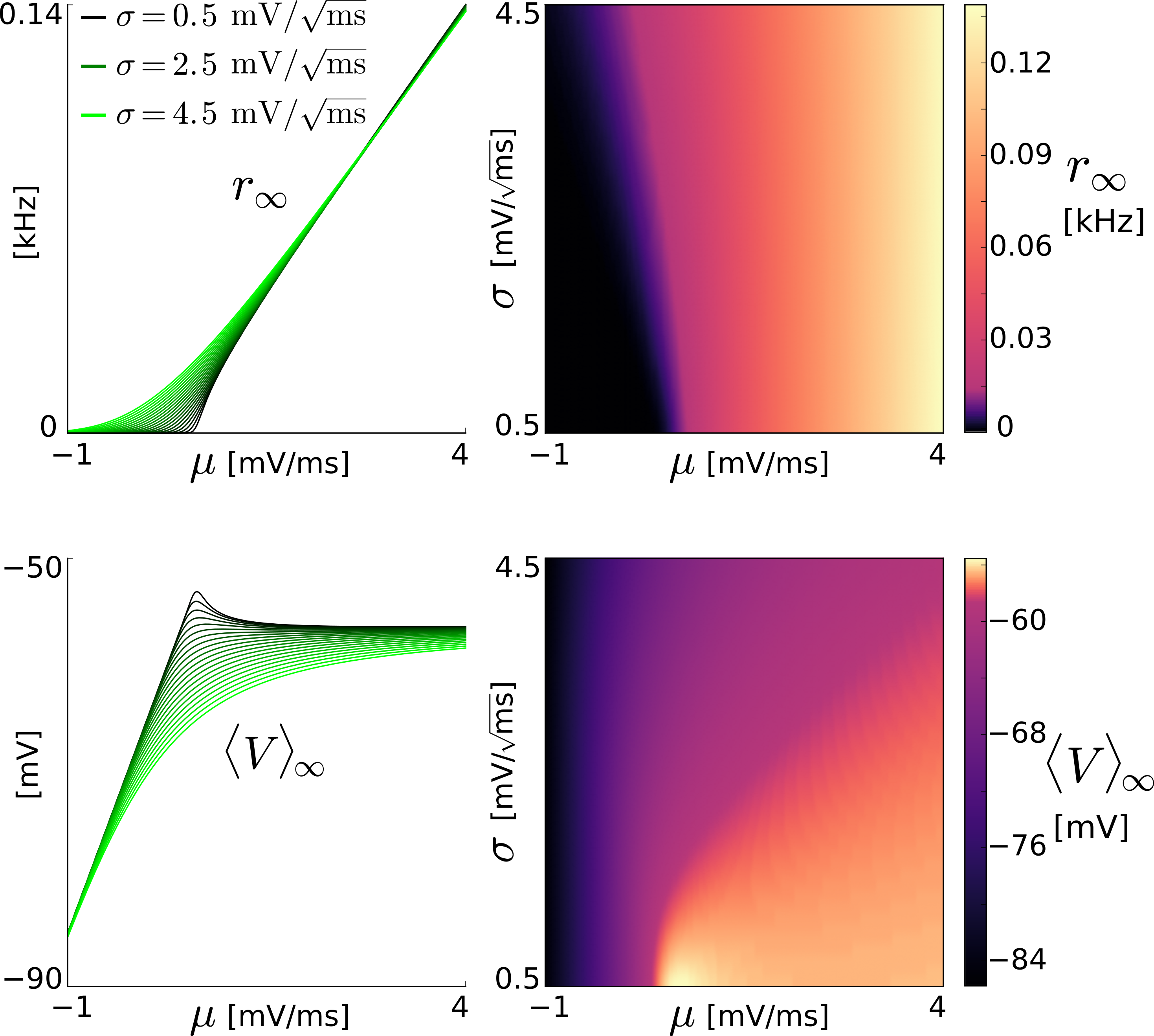
Figure 6: Steady-state spike rate and mean membrane voltage for a population of EIF neurons. $r_{\infty}$ and $\langle V\rangle_{\infty}$ for an uncoupled population of EIF neurons (aEIF with $a=b=0$) as a function of (generic) input mean $\mu$ and standard deviation $\sigma$, calculated from the (steady-state) Fokker-Planck equation, shown in two different representations (left and right, each).

denotes the stationary value of Eq. (29) under replacement of the (time-varying) total moments $\mu_{\mathrm{tot}}$ and $\sigma_{\mathrm{tot}}^{2}$ in the probability flux $q_{p}$, Eq. (25), by (constants) $\mu$ and $\sigma^{2}$, respectively. Thus the steady-state spike rate $r_{\infty}$ effectively corresponds to that of an uncoupled EIF population whose membrane voltage is governed by $dV_{i}/dt=[I_{\mathrm{L}}(V_{i})+I_{\mathrm{exp}}(V_{i})]/C+\mu+\sigma\xi_{i}(t)$ plus reset condition, i.e., adaptation and synaptic current dynamics are detached. For a visualization of $r_{\infty}(\mu,\sigma)$ see Fig. 6.

When simulating the reduced models these quantities need to be evaluated for each discrete time point $t$ at a certain value of $(\mu,\sigma)$ which depends on the overall synaptic moments $\mu_{\mathrm{syn}}(t)$, $\sigma_{\mathrm{syn}}^{2}(t)$ and on the mean adaptation current $\langle w\rangle(t)$ in a model-specific way (as described in the following Sects.). An example trajectory of $r_{\infty}$ in the $(\mu,\sigma)$ space for a network showing stable spike rate oscillations is shown in Fig. 5.

Importantly, these quantities depend on the parameters of synaptic input ($J$, $K$, $\tau_{d}$, $\mu_{\mathrm{ext}}$, $\sigma_{\mathrm{ext}}$) and adaptation current ($a$, $b$, $\tau_{w}$, $E_{w}$) only through their arguments $(\mu,\sigma)$. Therefore, for given parameter values of the EIF model ($C$, $g_{\mathrm{L}}$, $E_{\mathrm{L}}$, $\Delta_{\mathrm{T}}$, $V_{\mathrm{T}}$, $V_{\mathrm{r}}$, $T_{\mathrm{ref}}$) we precalculate those quantities on a (reasonably large and sufficiently dense) grid of $\mu$ and $\sigma$ values, and access them during time integration by interpolating the quantity values stored in a table. This greatly reduces the computational complexity and enables rapid numerical simulations.

The derived low-dimensional models describe the spike rate dynamics and generally do not express the evolution of the entire membrane voltage distribution. Therefore, the mean adaptation dynamics, which depends on the density $p(V,t)$ (via $\langle V\rangle$, cf. Eq. (23)) is adjusted through approximating the mean membrane voltage $\langle V\rangle$ by the expectation over the steady-state distribution,

$$\langle V\rangle_{\infty}=\frac{\int_{-\infty}^{V_{\mathrm{s}}}vp_{\infty}(v)dv}{\int_{-\infty}^{V_{\mathrm{s}}}p_{\infty}(v)dv},$$ (38)

which is valid for sufficiently slow adaptation current dynamics [48, 58]. The steady-state distribution is defined as $p_{\infty}(V)=\lim_{t\to\infty}p(V,t;\mu_{\mathrm{tot}}\!=\!\mu,\sigma_{\mathrm{tot}}\!=\!\sigma)$, representing the stationary membrane voltages of an uncoupled EIF population for generic input mean $\mu$ and standard deviation $\sigma$. The mean adaptation current in all reduced models is thus governed by

$$\frac{d{\langle w\rangle}}{dt}=\frac{a\left(\langle V\rangle_{\infty}-E_{w}\vphantom{{}^{2}}\right)-\langle w\rangle}{\tau_{w}}+b\,r(t),$$ (39)

where the evaluation of quantity $\langle V\rangle_{\infty}$ in terms of particular values for $\mu$ and $\sigma$ at a given time $t$ is model-specific (cf. following Sects.). Note again that the calculation of $\langle V\rangle_{\infty}$ slightly changes when considering an (optional) spike shape extension for the aEIF model, as described at the end of the Methods section.

The Fokker-Planck model does not restrict the form of the delay distribution $p_{d}$, except that the convolution with the spike rate $r$, Eq. (20), has to be well defined. Here, however, we aim at specifying the complete network dynamics in terms of a low-dimensional ODE system. Exploiting the exponential form of the delay distribution $p_{d}$ we obtain a simple ordinary differential equation for the delayed spike rate,

$$\frac{dr_{d}}{dt}=\frac{r-r_{d}}{\tau_{d}},$$ (40)

which is equivalent to the convolution $r_{d}=r\ast p_{d}$.

Note that more generally any delay distribution from the exponential family allows to represent the delayed spike rate $r_{d}$ by an equivalent ODE instead of a convolution integral [68]. Identical delays, $r_{d}(t)=r(t-d)$, are also possible but lead to delay differential equations. Naturally, in case of no delays, we simply have $r_{d}(t)=r(t)$.

To simulate the reduced models standard explicit time discretization schemes can be applied – directly to the first order equations of the LN_exp model, and for the other models (LN_dos, spec₁, spec₂) – to the respective equivalent (real) first order systems. We would like to note that when using the explicit Euler method to integrate any of the latter three low-dimensional models a sufficiently small integration time step $\Delta t$ is required to prevent oscillatory artifacts. Although the explicit Euler method works well for the parameter values used in this contribution, we have additionally implemented the method of Heun, i.e., the explicit trapezoidal rule, which is second order accurate.

Spectral models

Eigendecomposition of the Fokker-Planck operator

Following and extending [18] we can specify the Fokker-Planck operator $\mathcal{L}$

$$\mathcal{L}(\mu,\sigma)[p]=-\frac{\partial}{\partial V}\left[\left(\frac{I_{\mathrm{L}}(V)+I_{\mathrm{exp}}(V)}{C}+\mu\right)p\right]+\frac{\sigma^{2}}{2}\frac{\partial^{2}p}{\partial V^{2}},$$ (41)

for an uncoupled EIF population receiving (constant) input $(\mu,\sigma)$, cf. Sect. Low-dimensional approximations. This operator allows to rearrange the FP dynamics of the recurrent aEIF network, Eq. (24), as

$$\frac{\partial p}{\partial t}=\mathcal{L}(\mu_{\mathrm{tot}}(t),\sigma_{\mathrm{tot}}(t))[p]$$ (42)

which depends on the (time-varying) total input moments $\mu_{\mathrm{tot}}(t,r_{d},\langle w\rangle)$ and $\sigma_{\mathrm{tot}}^{2}(t,r_{d})$, cf. Eq. (26),(27), in the drift and diffusion coefficients, respectively.

For each value of $(\mu,\sigma)$ the operator $\mathcal{L}$ possesses an infinite, discrete set of eigenvalues $\lambda_{n}$ in the left complex half-plane including zero [18], i.e., $\mathrm{Re}\{\lambda_{n}\}\leq 0$, and associated eigenfunctions $\phi_{n}(V)$ ($n=0,1,2,\dots$) satisfying

$$\mathcal{L}[\phi_{n}]=\lambda_{n}\phi_{n}.$$ (43)

Furthermore, the boundary conditions, Eq. (30)–(32) have to be fulfilled for each eigenfunction $\phi_{n}$ separately, i.e., the absorbing boundary at the spike voltage,

$$\phi_{n}(V_{\mathrm{s}})=0,$$ (44)

and the reflecting barrier at the (finite) lower bound voltage,

$$q_{\phi_{n}}(V_{\mathrm{lb}})=0,$$ (45)

must hold. The eigenflux is given by

$$q_{\phi_{n}}(V)=\left(\frac{I_{\mathrm{L}}(V)+I_{\mathrm{exp}}(V)}{C}+\mu\right)\phi_{n}(V)-\frac{\sigma^{2}}{2}\frac{\partial}{\partial V}\phi_{n}(V),$$ (46)

i.e., the flux $q_{p}$ of Eq. (25) with eigenfunction $\phi_{n}$ and (constant) generic input moments ($\mu,\sigma^{2}$) instead of density $p$ and (time-varying) total input moments, respectively. Moreover, the eigenflux $q_{\phi_{n}}$ has to be reinjected into the reset voltage, cf. Eq. (30),

$$q_{\phi_{n}}(V_{\mathrm{r}}^{+})-q_{\phi_{n}}(V_{\mathrm{r}}^{-})=q_{\phi_{n}}(V_{\mathrm{s}}),$$ (47)

where we have neglected the refractory period, i.e., $T_{\mathrm{ref}}=0$. Note that incorporating a refractory period $T_{\mathrm{ref}}>0$ is straightforward only for the simplified case of vanishing total input moment variations, $\dot{\mu}_{\mathrm{tot}}\approx\dot{\sigma^{2}_{\mathrm{tot}}\mkern-14.0mu}\mkern 14.0mu\approx 0$, which is described in the following section and is not captured here in general.

The spectrum of $\mathcal{L}$ is shown in Fig. 7A and further discussed in Sect. Remarks on the spectrum.

Defining the non-conjugated[69] inner product $\langle\psi,\phi\rangle=\int_{V_{\mathrm{lb}}}^{V_{\mathrm{s}}}\psi(v)\phi(v)dv$ yields the corresponding adjoint operator $\mathcal{L}^{*}(\mu,\sigma)$ given by [18]

$$\mathcal{L}^{*}=\left(\frac{I_{\mathrm{L}}(V)+I_{\mathrm{exp}}(V)}{C}+\mu\right)\frac{\partial}{\partial V}+\frac{\sigma^{2}}{2}\frac{\partial^{2}}{\partial V^{2}},$$ (48)

which satisfies $\langle\psi,\mathcal{L}\phi\rangle=\langle\mathcal{L}^{*}\psi,\phi\rangle$ for any complex-valued functions $\psi$ and $\phi$ that are sufficiently smooth on $[V_{\mathrm{lb}},V_{\mathrm{s}}]$. $\mathcal{L}^{*}$ has the same set of eigenvalues $\lambda_{n}$ as $\mathcal{L}$ but distinct associated eigenfunctions $\psi_{n}(V)$, i.e.,

$$\mathcal{L}^{*}[\psi_{n}]=\lambda_{n}\psi_{n},$$ (49)

which have to satisfy three boundary conditions,

$$\psi_{n}(V_{\mathrm{s}})=\psi_{n}(V_{\mathrm{r}}),$$ (50)

$$\frac{\partial\psi_{n}}{\partial V}(V_{\mathrm{lb}})=0,$$ (51)

$$\frac{\partial\psi_{n}}{\partial V}(V_{\mathrm{r}}^{+})=\frac{\partial\psi_{n}}{\partial V}(V_{\mathrm{r}}^{-})$$ (52)

that are determined by integrating $\langle\psi_{n},\mathcal{L}[\phi_{n}]\rangle$ by parts and equalling with $\langle\mathcal{L}^{*}[\psi_{n}],\phi_{n}\rangle$ using the conditions of $\mathcal{L}$, Eqs. (44)–(47). Note that the last condition, Eq. (52), ensures a continuous derivative of $\psi_{n}$ at $V_{\mathrm{r}}$ in contrast to the eigenfunctions $\phi_{n}$ of $\mathcal{L}$, that have a kink at the reset due to reinjection condition, Eq. (47), as shown in Fig. 7B.

The eigenfunctions of $\mathcal{L}$ and $\mathcal{L}^{*}$ are pairwise orthogonal and in the following (without loss of generality) assumed to be scaled according to the biorthonormality condition,

$$\langle\psi_{n},\phi_{m}\rangle=\delta_{nm}.$$ (53)

The membrane voltage probability density can now be expanded onto the (moving) eigenbasis of $\mathcal{L}$ [18, 70],

$$p(V,t)=\sum_{n=0}^{\infty}\alpha_{n}(t)\phi_{n}(V),$$ (54)

where each eigenfunction $\phi_{n}$ depends on time via the total input moments $\mu=\mu_{\mathrm{tot}}(t,r_{d},\langle w\rangle)$, $\sigma^{2}=\sigma^{2}_{\mathrm{tot}}(t,r_{d})$, and the projection coefficients are given by $\alpha_{n}=\langle\psi_{n},p\rangle$ and particularly $\alpha_{0}=1$ [18]. Deriving $\alpha_{n}$ with respect to time (for $n=1,2,\dots$) and using the expansion, Eq. (54), the Fokker-Planck Eq. (42) as well as the definition of the adjoint operator yields an infinite-dimensional equation for the complex-valued projection coefficients $\boldsymbol{\alpha}(t)=(\alpha_{1}(t),\,\alpha_{2}(t),\,\dots)^{T}$,

$$\dot{\boldsymbol{\alpha}}=\left(\mathbf{\Lambda}+\mathbf{C}_{\mu}\,\dot{\mu}_{\mathrm{tot}}+\mathbf{C}_{\sigma^{2}}\,\dot{\sigma^{2}_{\mathrm{tot}}\mkern-14.0mu}\mkern 14.0mu\right)\boldsymbol{\alpha}+\mathbf{c}_{\mu}\,\dot{\mu}_{\mathrm{tot}}+\mathbf{c}_{\sigma^{2}}\,\dot{\sigma^{2}_{\mathrm{tot}}\mkern-14.0mu}\mkern 14.0mu.$$ (55)

This dynamics is initialized by $\alpha_{n}(0)=\langle\psi_{n},p_{0}\rangle$, and is complemented by (i) an expression for the spike rate,

$$r(t)=r_{\infty}+\mathbf{f}\cdot\boldsymbol{\alpha},$$ (56)

that is obtained from Eq. (29) (using Eq. (54)), and (ii) by the mean adaptation and delayed spike rate dynamics, Eqs. (39),(40). The dots in Eqs. (55) and (56) denote time derivatives (e.g.,, $\dot{\sigma^{2}_{\mathrm{tot}}\mkern-14.0mu}\mkern 14.0mu=d\sigma^{2}_{\mathrm{tot}}/dt$) and a non-conjugated scalar product of complex vectors (i.e., $\mathbf{f}\cdot\boldsymbol{\alpha}=\sum_{n=1}^{\infty}f_{n}\alpha_{n}$), respectively. The matrix $\mathbf{\Lambda}=\mathrm{diag}(\lambda_{1},\lambda_{2},\dots)$ contains the eigenvalues of $\mathcal{L}$, the matrices $\mathbf{C}_{\mu}$ and $\mathbf{C}_{\sigma^{2}}$ have elements $(\mathbf{C}_{x})_{n,m}=\langle\partial_{x}\psi_{n},\,\phi_{m}\rangle$ for $x\in\{\mu,\sigma^{2}\}$ and $n,m\in\mathbb{N}$ with partial derivative $\partial_{x}=\partial/\partial x$, the vectors $\mathbf{c}_{\mu}$ and $\mathbf{c}_{\sigma^{2}}$ consist of components $c^{x}_{n}=\langle\partial_{x}\psi_{n},\,\phi_{0}\rangle$. The steady-state spike rate is given by $r_{\infty}=q_{\phi_{0}}(V_{\mathrm{s}})$, i.e., the flux of the eigenfunction $\phi_{0}=p_{\infty}$ that represents the stationary membrane voltage distribution $p_{\infty}$ and corresponds to the (stationary) eigenvalue $\lambda_{0}=0$ [18]. The vector $\mathbf{f}$ contains the (nonstationary) eigenfluxes evaluated at the spike voltage, $f_{n}=q_{\phi_{n}}(V_{\mathrm{s}})$.

Note that the quantities ($\mathbf{\Lambda},\mathbf{C}_{\mu},\mathbf{C}_{\sigma^{2}},\mathbf{c}_{\mu},\mathbf{c}_{\sigma^{2}},r_{\infty},\mathbf{f}$, $\langle V\rangle_{\infty}$) all depend on time in Eqs. (55),(56),(39) via the total input moments $(\mu_{\mathrm{tot}},\sigma_{\mathrm{tot}}^{2})$. Particularly, at time $t$ the (biorthonormal) solution of the eigenvalue problems for $\mathcal{L}$ and its adjoint $\mathcal{L}^{*}$, Eqs. (43)–(47) and (49)–(52) with $n\in\mathbb{N}_{0}$, is required for $\mu=\mu_{\mathrm{tot}}(t,r_{d},\langle w\rangle)$, $\sigma=\sigma_{\mathrm{tot}}(t,r_{d})$. Because $\mathcal{L}$ is a real operator its spectrum contains only real eigenvalues and/or complex conjugated pairs depending on $(\mu,\sigma)$. This property carries over to the eigenfunctions and therefore also to the components of all quantities above implying for example that the scalar product $\mathbf{f}\cdot\boldsymbol{\alpha}$ is always real-valued.

Although the spectral representation, Eqs. (55),(56), is fully equivalent to the original (partial differential) Fokker-Planck equation without refractory period and while it contains only time derivatives it is still an infinite-dimensional and furthermore generally an implicit model. Therefore, to derive an explicit low-dimensional ordinary differential model for the spike rate $r(t)$, it is not sufficient to truncate the expansion in Eq. (54) after, e.g., two terms but additional assumptions have to be considered.

Basic model: one eigenvalue, negligible input variations

The first and simpler, derived spectral model is based on [19] and requires the strong assumption of vanishing changes of the total input moments, $\dot{\mu}_{\mathrm{tot}}\approx 0$, $\dot{\sigma^{2}_{\mathrm{tot}}\mkern-14.0mu}\mkern 14.0mu\approx 0$. Under this approximation the projection coefficient dynamics, Eq. (55), simplifies to

$$\dot{\alpha}_{n}=\lambda_{n}\alpha_{n}$$ (57)

for $n\in\mathbb{N}$. Considering only the dominant (nonzero) eigenvalue

$$\lambda_{1}=\mathrm{argmin}\{|\mathrm{Re}\{\lambda_{n}\}|:\lambda_{n}\neq 0\},$$ (58)

i.e., the “slowest mode”, we obtain from Eqs. (56) and (57) that $r(t)=r_{\infty}+m_{1}\,\mathrm{Re}\{f_{1}\alpha_{1}\}$ with $m_{1}=1$ if $\lambda_{1}\in\mathbb{R}$ and $m_{1}=2$ if $\lambda_{1}\in\mathbb{C}\setminus\mathbb{R}$. Here we have included for a complex eigenvalue $\lambda_{1}$ also its complex conjugate $\overline{\lambda}_{1}$ that has the projection coefficient $\overline{\alpha_{1}}(t)$. They jointly yield a zero imaginary part in the scalar product of Eq. (56). Defining $\tilde{r}(t)=r_{\infty}+m_{1}f_{1}\alpha_{1}$ yields the complex first order equation for the spike rate [19],

$$\dot{\tilde{r}}=\lambda_{1}(\tilde{r}-r_{\infty}),\qquad r(t)=\mathrm{Re}\{\tilde{r}\}.$$ (59)

While this derivation is based on neglecting changes of the total input moments, their time-variation is effectively reintroduced in the two quantities (dominant eigenvalue and steady-state rate), i.e., $\lambda_{1}(\mu_{\mathrm{tot}},\sigma_{\mathrm{tot}})$ and $r_{\infty}(\mu_{\mathrm{tot}},\sigma_{\mathrm{tot}})$ with $\mu_{\mathrm{tot}}(t)$ and $\sigma_{\mathrm{tot}}(t)$ according to Eqs. (26),(27). Therefore, the spike rate evolution, Eq. (59), is complemented with the dynamics of mean adaptation current $\langle w\rangle$ and delayed spike rate $r_{d}$, Eqs. (39),(40), where the former involves the third $(\mu_{\mathrm{tot}},\sigma_{\mathrm{tot}})$-dependent quantity $\langle V\rangle_{\infty}$. See Figs. 6,7C for the involved quantities depending on (generic) input $\mu$, $\sigma$.

We call this first derived low-dimensional spike rate model, i.e., Eqs. (59), (39),(40), spec₁. It is very simple in comparison with the full Fokker-Planck system in the spectral representation, Eqs. (55)–(56), (39),(40), in the sense that it does not depend on “nonstationary” quantities of $\mathcal{L}$ or its adjoint $\mathcal{L}^{*}$ except for the dominant eigenvalue $\lambda_{1}$.

Note that under the assumption of vanishing input moment variations the dynamics of the expansion coefficients $\alpha_{n}$, Eq. (55), is simply exponentially decaying in time, cf. Eq. (57). This allows to incorporate a refractory period $T_{\mathrm{ref}}>0$ into the spectral decomposition framework by inserting the eigenbasis expansion of the membrane voltage distribution, Eq. (54), into the reinjection condition of the Fokker-Planck model, Eq. (30), using $\alpha_{n}(t)=\alpha_{n}(0)\exp(\mathbf{\lambda}_{n}t)$ and the absorbing boundary, Eq. (44). This generalizes the reinjection condition for the eigenfunctions $\phi_{n}$ of $\mathcal{L}$ from Eq. (47) to

$$q_{\phi_{n}}(V_{\mathrm{r}}^{+})-q_{\phi_{n}}(V_{\mathrm{r}}^{-})=q_{\phi_{n}}(V_{\mathrm{s}})\exp(-\lambda_{n}T_{\mathrm{ref}}),$$ (60)

which was applied in [19], and the corresponding boundary condition for the adjoint operator’s eigenfunctions $\psi_{n}$ from Eq. (50) to

$$\psi_{n}(V_{\mathrm{s}})=\psi_{n}(V_{\mathrm{r}})\exp(-\lambda_{n}T_{\mathrm{ref}}).$$ (61)

Advanced model: two eigenvalues, slow input moment variations

Another possibility to derive a low-dimensional spike rate model is based on ongoing work of Maurizio Mattia. He has recognized that under the weaker (compared to the basic spec₁ model above) assumption of small but not vanishing input moment changes a real-valued second order ordinary differential equation for the spike rate $r(t)$ can be consistently derived [20]. Here we extend this approach to account for neuronal adaptation, time-varying external input moments and delay distributions.

The steps in a nutshell (for the detailed derivation see S1 Text) are (i) taking the derivative of Eq. (55) (once) and of (56) (twice) w.r.t. time, (ii) considering only the first two dominant eigenvalues $\lambda_{1}$ and $\lambda_{2}$, i.e., neglecting all (faster) eigenmodes that correspond to eigenvalues with larger absolute real part (“modal approximation”), (iii) assuming slowly changing input moments, i.e., small $\dot{\mu}_{\mathrm{tot}}$ and $\dot{\sigma^{2}_{\mathrm{tot}}\mkern-14.0mu}\mkern 14.0mu$ that allow to consider projections coefficients of that order, i.e., $\alpha_{n}=\mathcal{O}(\dot{\mu}_{\mathrm{tot}})$ and $\alpha_{n}=\mathcal{O}(\dot{\sigma^{2}_{\mathrm{tot}}\mkern-14.0mu}\mkern 14.0mu)$ for $n=1,2$, and therefore to consider only linear occurences of $\dot{\mu}_{\mathrm{tot}}$, $\dot{\sigma^{2}_{\mathrm{tot}}\mkern-14.0mu}\mkern 14.0mu$, $\alpha_{1}$, $\alpha_{2}$, and neglect terms of second and higher order. The slowness approximation implies that neither the external moments $\mu_{\mathrm{ext}}(t)$, $\sigma^{2}_{\mathrm{ext}}(t)$ nor the (delayed) spike rate $r_{d}(t)$ nor the population-averaged adaptation current $\langle w\rangle(t)$ should change very fast (cf. Eqs. (26),(27),(21)). Note that the dynamics of $\langle w\rangle$ is assumed to be slow already, cf. Sect. Fokker-Planck system.

Under these approximations we obtain for the spike rate dynamics the following real second order ODE,

$$\beta_{2}\,\ddot{r}+\beta_{1}\,\dot{r}+\beta_{0}\,r=r_{\infty}-r-\beta_{c},$$ (62)

that is complemented with the mean adaptation current and delayed spike rate dynamics, Eqs. (39),(40), and we call the model spec₂. The coefficients

$$\beta_{2}= \,\,D,$$ (63)

$$\beta_{1}= \,-T+DM\frac{b}{C}-\frac{R}{\tau_{d}},$$ (64)

$$\beta_{0}= -DM\frac{b}{\tau_{w}C}-\frac{b}{C}H_{\mu}+\frac{1}{\tau_{d}}\left(KJH_{\mu}+KJ^{2}H_{\sigma^{2}}\right)+\frac{R}{\tau_{d}^{2}},$$ (65)

$$\beta_{\text{c}}= \,\,r_{d}\left(-\frac{1}{\tau_{d}}\left(KJH_{\mu}+\,KJ^{2}H_{\sigma^{2}}\right)-\frac{R}{\tau_{d}^{2}}\right)$$

$$-\left(\ddot{\mu}_{\text{ext}}+\frac{a\left(\langle V\rangle_{\infty}-E_{w}\right)-\langle w\rangle}{\tau_{w}^{2}C}\right)DM-\ddot{\sigma^{2}_{\text{ext}}\mkern-14.0mu}\mkern 14.0muDS$$ (66)

$$+\left(\dot{\mu}_{\text{ext}}-\frac{a\left(\langle V\rangle_{\infty}-E_{w}\right)-\langle w\rangle}{\tau_{w}C}\right)H_{\mu}+\dot{\sigma^{2}_{\text{ext}}\mkern-14.0mu}\mkern 14.0muH_{\sigma^{2}},$$

depend on the (lumped) quantities $D=1/\lambda_{1}\cdot 1/\lambda_{2}$, $T=1/\lambda_{1}+1/\lambda_{2}$, $M=\partial_{\mu}r_{\infty}+\mathbf{f}\cdot\mathbf{c}_{\mu}$, $S=\partial_{\sigma^{2}}r_{\infty}+\mathbf{f}\cdot\mathbf{c}_{\sigma^{2}}$, $R=DMKJ+DSKJ^{2}$, $H_{\mu}=TM+DMa\partial_{\mu}\langle V\rangle_{\infty}/(\tau_{w}C)-DF_{\mu}$, $H_{\sigma^{2}}=TS+DMa\partial_{\sigma^{2}}\langle V\rangle_{\infty}/(\tau_{w}C)-DF_{\sigma^{2}}$, $F_{\mu}=\mathbf{f}\cdot\mathbf{\Lambda}\,\mathbf{c}_{\mu}$ and $F_{\sigma^{2}}=\mathbf{f}\cdot\mathbf{\Lambda}\,\mathbf{c}_{\sigma^{2}}$. Here the diagonal eigenvalue matrix $\mathbf{\Lambda}=\mathrm{diag}(\lambda_{1},\lambda_{2})$ and the vectors $\mathbf{f}=(f_{1},f_{2})^{T}$, $\mathbf{c}_{\mu}=(c^{\mu}_{1},c^{\mu}_{2})^{T}$, $\mathbf{c}_{\sigma^{2}}=(c^{\sigma^{2}}_{1},c^{\sigma^{2}}_{2})^{T}$ are two-dimensional in contrast to infinite as in the original dynamics, Eqs. (55) and (56). These individual quantities, that also include $\langle V\rangle_{\infty}$ (cf. Eq. (39)), $r_{\infty}$ and derivatives of both w.r.t. generic mean $\mu$ and variance $\sigma^{2}$, are evaluated at the total input moments $\mu=\mu_{\mathrm{tot}}(t,r_{d},\langle w\rangle)$, $\sigma^{2}=\sigma_{\mathrm{tot}}^{2}(t,r_{d})$. A relevant subset of individual and lumped quantities is shown in Figs. 6,7C.

The four coefficients, Eqs. (63)–(66), are real-valued because we define $\lambda_{2}$ as the second dominant eigenvalue conditioned that $(\lambda_{1},\lambda_{2})$ compose either a real or a complex conjugated eigenvalue pair, i.e.,

$$\lambda_{2}=\mathrm{argmin}\{|\mathrm{Re}\{\lambda_{n}\}|\,:\,\lambda_{n}\neq\lambda_{1}\ \ \text{s.t.}\ \ \lambda_{n}\neq 0,\ \lambda_{1}+\lambda_{n}\in\mathbb{R}\},$$ (67)

where $\lambda_{1}$ is obtained as for the (basic) spec₁ model, cf. Eq. (58). This condition ensures that all related complex quantities occur in vectors of two complex conjugate components (for example, $f_{1}=\overline{f_{2}}$) implying that the scalar products above are real-valued (e.g., $\mathbf{f}\cdot\mathbf{c}_{\mu}\in\mathbb{R}$) and therefore all (nine) lumped quantities, too. Note that this specific definition of $\lambda_{2}$ is required only for integrate-and-fire neuron models that have a lower bound different from the reset, i.e., $V_{\mathrm{lb}}<V_{\mathrm{r}}$, as discussed in the following section.

The coefficients of the spec₂ model require – in addition to eigenvalues $\lambda_{n}$ and steady-state rate $r_{\infty}$ (cf. basic spec₁ model, Eq. (59)) – quantities that involve the first and second eigenfunctions of the Fokker-Planck operator $\mathcal{L}$ and its adjoint $\mathcal{L}^{*}$. Additionally, $\beta_{1}$, $\beta_{0}$ and $\beta_{c}$ contain the parameters of membrane voltage ($C$) and mean adaptation current dynamics ($a$, $b$, $\tau_{w}$, $E_{w}$) as well as of the recurrent coupling ($K$, $J$, $\tau_{d}$) and, importantly, explicit dependencies on the population-averaged adaptation current $\langle w\rangle$ and the delayed spike rate $r_{d}$ (that is in addition to implicitly via $\mu_{\mathrm{tot}}$ and $\sigma_{\mathrm{tot}}$). Furthermore $\beta_{c}$ depends on the first two time derivatives of the external input moments $\mu_{\mathrm{ext}}(t)$ and $\sigma^{2}_{\mathrm{ext}}(t)$. This explicit occurence of neuronal and coupling parameters, state variables and input moment derivatives in the coefficients is not expressed in the basic spectral model (spec₁), Eq. (59). A consequence is that for the (advanced) model spec₂ the external moments have to be provided twice differentiable or in case of non-smooth time series to be filtered (e.g., see Sect. Performance for variations of the mean input).

The particular coefficients, Eqs. (63)–(66), are specific for the choice of an exponential delay distribution, as indicated by the occurrence of the mean delay $\tau_{d}$ in $\beta_{1}$, $\beta_{0}$ and $\beta_{c}$. Other choices such as identical delays or no delays are described in the supplementary material S1 Text.

Note that the original (infinite-dimensional) spectral dynamics, Eq. (55),(56), assumes for the refractory period a value of $T_{\mathrm{ref}}=0$ which carries over to the same choice for the spec₂ model, whereas $T_{\mathrm{ref}}>0$ is not supported (yet).

The spike rate is by definition nonnegative, however, the model spec₂, Eq. (62), can yield negative rates $r(t)$, especially for small total mean input $\mu_{\mathrm{tot}}$ and fast (external) input changes, e.g., when $\dot{\mu}_{\mathrm{ext}}$ is large. We explicitly avoid that behaviour by setting both the spike rate of this model, $r$, and its derivative, $\dot{r}$, to zero whenever $r(t)<0$ and continue the integration of the differential equation afterwards.

Remarks on the spectrum

In the previous two sections we have developed two spike rate models based on approximations of the Fokker-Planck system’s spectral representation, Eqs. (55),(56) under different slowness assumptions. In the derivation of the (simple) model spec₁, cf. Eq. (59), temporal variations of the total input moments are completely neglected while the (advanced) model spec₂, cf. Eq. (62), incorporates (slow) changes of the total input moments through linear terms (proportional to $\dot{\mu}_{\mathrm{tot}}$ or $\dot{\sigma^{2}_{\mathrm{tot}}\mkern-14.0mu}\mkern 14.0mu$) and neglects (faster) quadratic and higher order ones.

Both slowness approximations imply that the eigenvalue matrix $\boldsymbol{\Lambda}$ is the dominant term in the homogeneous part of Eq. (55). Therefore the eigenvalues approximately correspond to decay time constants $1/|\mathrm{Re}\{\lambda_{n}\}|$ in their real part and in case of complex eigenvalues they contribute damped oscillatory components with frequency $|\mathrm{Im}\{\lambda_{n}\}|/(2\pi)$ through their imaginary part to the dynamics. How the spectrum of the Fokker-Planck operator $\mathcal{L}$ depends on the input moments therefore gives insights into the behavior of the derived spike rate models spec₁ and spec₂, and of the FP model with slow adaptation in general.

Here we summarize the main properties of the eigenvalues $\lambda_{n}(\mu,\sigma)$ for the (uncoupled, nonadaptive) EIF neuron model as a function of generic input mean $\mu$ and standard deviation $\sigma$ (cf. Sect. Low-dimensional approximations) that are shown in Fig. 7A. Note that at time $t$ the total input determines the particularly effective eigenvalue, $\lambda_{n}(\mu_{\mathrm{tot}}(t),\sigma_{\mathrm{tot}}(t))$, in dependence of external input moments, (delayed) spike rate and adaptation current, cf. Eqs. (26),(27),(21). We thereby extend the findings of [18] concerning the perfect integrate-and-fire neuron with reflecting lower barrier at the reset voltage (PIFb), i.e., $dV_{i}/dt=\mu+\sigma\xi_{i}(t)$ with $V_{\mathrm{lb}}=V_{\mathrm{r}}$.

1. The eigenvalue $\lambda_{0}=0$ exists for all (generic) input moments $\mu$,$\sigma^{2}$ with stationary membrane voltage distribution as corresponding eigenfunction, $\phi_{0}=p_{\infty}$ (see Fig. 7A,B), the respective adjoint eigenfunction is constant, $\psi_{0}=1$, cf. [18]. The other, nonstationary eigenvalues $\lambda_{n}$ with $n\geq 1$ have negative real parts for all $(\mu,\sigma)$ which yields stability of the stationary distribution for constant total input moments. For sufficiently small mean input $\mu_{\mathrm{min}}$ the eigenvalues $\lambda_{n}(\mu_{\mathrm{min}},\sigma)$ are real-valued for all $n$ and $\sigma$, i.e., no (damped) oscillatory spike rate transient in that regime are present (consistent with [18]), cf. Fig. 7A.

2. Two classes of modes can be distinguished: eigenvalues of the first kind occur in couples which are real-valued at $\mu_{\mathrm{min}}$ but merge for increasing mean input $\mu$ to become a complex conjugated pair of decreasing absolute real part and almost linearly increasing imaginary part (see Fig. 7A). Thus they correspond in this situation to damped oscillatory dynamics with increased frequency $|\mathrm{Im}\{\lambda_{n}\}|/(2\pi)$ and decay time constant $1/|\mathrm{Re}\{\lambda_{n}\}|$ for stronger mean input. Note that there is no single critical parameter for the real-to-complex transition, instead that depends on the input mean $\mu$ and standard deviation $\sigma$ as well as on the eigenvalue index $n$ in contrast to the PIFb neuron where $\mu=0$ (alone) induces the transition [18]. We call this type of eigenvalue regular because it is observed also for very simple integrate-and-fire models (such as PIFb).
   The second type of eigenvalue is real for the whole input parameter space of $(\mu,\sigma)$. The corresponding decay time constant is large if noise dominates while for stronger mean input the respective dynamics is negligibly fast. Note that by setting the lower bound $V_{\mathrm{lb}}$ equal to the reset voltage, this eigenvalue class is completely removed for the EIFb model, which is the EIF membrane voltage description with $V_{\mathrm{lb}}=V_{\mathrm{r}}$ (not used here). This explains why this new type of eigenvalue has not been described in [18], and suggests a relationship to the diffusion of the membrane voltage for hyperpolarized neuronal states. The latter correspondence is further supported from the significant values of the respective eigenfunction $\phi_{n}$ below the reset voltage $V_{\mathrm{r}}$ in contrast to the eigenfunctions of regular eigenvalues (cf. Fig. 7B). Therefore we label this second type of eigenvalue diffusive.

3. The input noise intensity $\sigma$ controls the spectrum’s mixture of the two eigenvalue classes as follows: weak noise favors regular modes, i.e., the dominant two eigenvalues are pairs of real (for smaller mean input $\mu$) or complex conjugated eigenvalues (for larger $\mu$) while the diffusive modes are irrelevantly fast in this regime (cf. Fig. 7A, left). Increased input fluctuations, i.e., a larger $\sigma$, on the other hand leads to a spectrum with dominant (“slowest” eigenvalue $\lambda_{1}$) of the diffusive kind for small mean input $\mu$ while for larger $\mu$ the dominant mode is from the regular class (being real or complex depending on $\mu$, $\sigma$, $n$), see Fig. 7A, right. Furthermore an increased noise strength $\sigma$ leads to a smaller decay time constant $1/|\mathrm{Re}\{\lambda_{n}\}|$ for regular modes, i.e., their respective contribution to the spike rate dynamics is faster in the fluctuation-dominated regime than in the drift-dominated one, whereas for diffusive modes the opposite holds true.

The specific definition of the second dominant eigenvalue $\lambda_{2}$, Eq. (67), is necessary to ensure real coefficients in the spec₂ model, Eqs. (63)–(66), for regions in $(\mu,\sigma)$-space where the first dominant eigenvalue $\lambda_{1}$ is of the (real) diffusive type and the second is part of a complex conjugate couple (for an example see Fig. 7A, right).

Extracting the required dominant eigenvalues $\lambda_{1}$ (for both spectral models: spec₁, spec₂) and $\lambda_{2}$ (for spec₂ model only) according to Eqs. (58),(67) in the $(\mu,\sigma)$-plane leads to points of instantaneous changes in the imaginary part ($\lambda_{1}$ and $\lambda_{2}$) and the real part (only $\lambda_{2}$) due to transitions from a dominant diffusive mode for small mean input $\mu$ to a regular eigenvalue (or pair) becoming dominant for larger $\mu$ (see Fig. 7A,C and the last property above). These discontinuities (which lie on a one-dimensional curve $\mu(\sigma)$) could be avoided by either restricting to $V_{\mathrm{lb}}=V_{\mathrm{r}}$ (no diffusive modes) or by deriving a third spectral model based on three eigenvalues: the dominant regular pair together with the dominant diffusive eigenvalue. Making the latter extension is straightforward by using the same steps and slowness approximation as for the model spec₂ and would yield a 3rd order ODE for the spike rate $r(t)$ with smooth coefficients and is expected to show increased reproduction accuracy (especially for small mean input) compared to the model spec₂.

The properties above imply for the low-dimensional models spec₁ and spec₂, that both enable damped oscillatory spike rates for mean-dominated input (for large $\mu$) since then the first two dominant eigenvalues ($\lambda_{1}$ and $\lambda_{2}$) have nonzero imaginary parts and are complex conjugates of each other (see Fig. 7C). Furthermore in this case the effective time constant, $1/|\mathrm{Re}\{\lambda_{1}\}|=1/|\mathrm{Re}\{\lambda_{2}\}|$, is large (especially for small input standard deviation $\sigma$). For noise-dominated input, i.e., when $\sigma$ (and not $\mu$) is large, on the other hand, the corresponding spike rate dynamics is fast and does not contain an oscillatory component.

Numerical solver

Here we present a numerical solution method of the Fokker-Planck boundary eigenvalue problem (BEVP) for the operator $\mathcal{L}(\mu,\sigma)$, Eqs. (43)–(47), and its adjoint $\mathcal{L}^{*}(\mu,\sigma)$, Eqs. (49)–(52). The solution of the two BEVPs in terms of eigenvalues $\lambda_{n}$ and associated (biorthonormal) eigenfunctions ($\phi_{n}(V)$, $\psi_{n}(V)$) as well as quantities that are derived from those and are required by the models spec₁ and spec₂, is obtained for a rectangle of the input mean $\mu$ and standard deviation $\sigma$ (see Sect. Low-dimensional Approximations). Note that the numerical method is not restricted to the EIF neuron model and supports other integrate-and-fire models as well (e.g., perfect, leaky or quadratic).

The eigenequation $\mathcal{L}(\mu,\sigma)[\phi]=\lambda\phi$, i.e., Eq. (43) (omitting the eigenvalue index $n$), represents a second order ODE (cf. Eq. (41)), that is equivalent to the following first order system for the eigenflux $q_{\phi}(V)$ and the eigenfunction $\phi(V)$,

$$-\frac{d}{dV}\begin{pmatrix}q_{\phi}\\ \phi\end{pmatrix}=\underbrace{\begin{pmatrix}0&\lambda\\ \frac{2}{\sigma^{2}}&-2\frac{g(V)+\mu}{\sigma^{2}}\end{pmatrix}}_{=\mathbf{A}}\begin{pmatrix}q_{\phi}\\ \phi\end{pmatrix}$$ (68)

with coefficient matrix $\mathbf{A}(V)$ that has a nonlinear component through $g(V)=[I_{\mathrm{L}}(V)+I_{\mathrm{exp}}(V)]/C$ that contains leak and exponential (membrane) currents. Here it was used the form of the eigenflux $q_{\phi}$ (cf. Eq. (46)), and that $\mathcal{L}(\mu,\sigma)[\phi]=-\partial_{V}q_{\phi}$ for generic input moments $\mu$ and $\sigma^{2}$ (cf. Eq. (41)).

Basically a direct discretization, e.g., by a finite difference approximation, of the membrane voltage derivatives in the system (68) can be applied. In combination with the boundary conds., Eqs. (44)–(47), this leads to a (sparse) matrix eigenvalue problem that allows for application of standard (Arnoldi iteration based) numerical solvers. However, the convergence properties of this approach are very poor in the sense that extremely small voltage steps $\Delta V$ have to be chosen for the finite differences. Thus, the technique is inefficient as huge systems appear or even inaccurate due to amplified round-off errors by ill-conditioned matrices.

Here we propose an alternative solution procedure which is based on a reformulation of the system (68) with corresponding boundary conditions, Eqs. (44)–(47), as a complex-valued algebraic root finding problem

$$\lambda\mapsto q_{\phi}(V_{\mathrm{lb}};\lambda)\overset{!}{=}0$$ (69)

whose solutions are the eigenvalues $\lambda_{n}$. To evaluate the nonlinear function (the left hand side of this equation) for an arbitrary $\lambda\in\mathbb{C}$ (not necessary an eigenvalue) Eq. (68) is integrated backward starting from the spike voltage $V_{\mathrm{s}}$ (initializing one component to satisfy the absorbing boundary cond., Eq. (44), i.e., $\phi(V_{\mathrm{s}})=0$, and another component that can be chosen arbitrarily, $q_{\phi}(V_{\mathrm{s}})\in\mathbb{C}\setminus\{0\}$, due to the linearity of the problem) via the reset $V_{\mathrm{r}}$ (where the reinjection cond., Eq. (47), is enforced, i.e., $q_{\phi}(V_{\mathrm{r}}^{-})=q_{\phi}(V_{\mathrm{r}}^{+})-q_{\phi}(V_{\mathrm{s}})$, which induces a discontinuity in $q_{\phi}$ at the reset voltage) finally to the lower bound voltage $V_{\mathrm{lb}}$. There, a nonzero value of $q_{\phi}(V_{\mathrm{lb}})\in\mathbb{C}$ indicates that $\lambda$ is not an eigenvalue since in this case $\phi(V)$ violates the reflecting boundary condition, Eq. (45). $q_{\phi}(V_{\mathrm{lb}})=0$ on the other hand shows that $\lambda$ is an eigenvalue with corresponding eigenfunction $\phi(V)$ and eigenflux $q_{\phi}(V)$. Note that when considering a nonzero refractory period the generalized version of the reinjection cond., Eq. (60), i.e., $q_{\phi}(V_{\mathrm{r}}^{-})=q_{\phi}(V_{\mathrm{r}}^{+})-q_{\phi}(V_{\mathrm{s}})e^{-\lambda T_{\mathrm{ref}}}$, is enforced instead of the expression above. The latter is only valid for the spec₁ model, Eq. (59) (see Sect. Basic model: one eigenvalue, negligible input variations) and makes the Fokker-Planck eigenvalue problem nonlinear due to the exponentiation of $\lambda$ in Eq. (60).

The (complex-valued) root finding problem, Eq. (69) can be solved numerically to yield a target eigenvalue $\lambda_{n}$ using an iterative procedure (for example a variant of Newton’s method) given that a sufficiently close initial approximation $\tilde{\lambda}_{n}\in\mathbb{C}$ is available. In our Python implementation we apply Powell’s hybrid method as implemented in MINPACK wrapped through SciPy [67] to the equivalent real system of the two variables $\mathrm{Re}\{\lambda\}$ and $\mathrm{Im}\{\lambda\}$.

Appropriate initial approximations $\tilde{\lambda}_{n}$ can be achieved (i) by exploiting that for sufficiently small generic mean input $\mu_{\mathrm{min}}$ all eigenvalues have zero imaginary part (see Sect. Remarks on the spectrum). In that case the eigenvalues are given by the roots $\{\lambda_{0},\lambda_{1},\dots\}$ of $q(V_{\mathrm{lb}};\lambda)$ – the one-dimensional function of the real-valued eigenvalue candidate $\lambda\in(-\infty,0]$ – which are obtained, for example, by (dense) evaluation of that function in a sufficiently large (sub)interval below zero. Furthermore (ii) all eigenvalues depend continuously on the (input) parameters $\mu$ and $\sigma$ (cf. Fig. 7A), i.e., for a small step in the respective parameter space the solution $\lambda_{n}$ of Eq. (69) for the last parametrization is a very good initial value $\tilde{\lambda}_{n}$ for the current parametrization. With this initialization the solution of Eq. (69) is typically found in a few steps of the chosen Newton-like method (see S1 Text for details).

To efficiently and accurately evaluate $q_{\phi}(V_{\mathrm{lb}};\lambda)$ in each iteration (of the root finding algorithm), we perform an exponential (backward) integration of the system (68). The resulting scheme is based on truncating the Magnus expansion of the exact solution after one term [71]. Here matrix exponential function evaluations of the form $\exp[\mathbf{A}(V)\Delta V]$ occur that are calculated using an analytic expression [72]. Note that ODE solvers that either do not exploit the linear structure of Eq. (68) at all (such as the explicit Euler method but also higher order Runge-Kutta methods) or utilize linearity only in one variable (e.g., [73]) have poor convergence behaviour and thus require very small step sizes $\Delta V$ due to the strong nonlinearity $g(V)$ as a consequence of the large value of the current $I_{\mathrm{exp}}$ close to $V_{\mathrm{s}}$ and significantly large absolute eigenvalues $|\lambda_{n}|$, respectively.

For more information on the numerical solver we refer to S1 Text, where details regarding the adjoint operator, the exponential integration, the initial eigenvalue determination and the (parallelized) treatment of the input parameters are included.

Cascade models

Linear-Nonlinear (LN) cascade models of neuronal activity are often applied in neuroscience, because they are simple and efficient, and the model components can be estimated using established experimental procedures [74, 75, 21]. Here we use the LN cascade as an ansatz to develop a low-dimensional model and we determine its components from the underlying Fokker-Planck model. This section builds upon [21] and extends that approach for recurrently coupled aEIF neurons; specifically, by taking into account an adaptation current and variations of the input variance. Furthermore, we consider an improved approximation of the derived linear filters and include an (optional) explicit description of the spike shape, cf. [23] (ch 4.2).

The cascade models considered here produce spike rate output by applying to the time-varying mean $\mu_{\mathrm{syn}}$ and standard deviation $\sigma_{\mathrm{syn}}$ of the (overall) synaptic input, cf. Eq. (21), separately a linear temporal filter, $D_{\mu}$ and $D_{\sigma}$, followed by a common nonlinear function $F$. That is,

$$r(t) =F\left(\mu_{\mathrm{f}},\sigma_{\mathrm{f}},\langle w\rangle\vphantom{{}^{2}}\right),$$ (70)

$$\mu_{\mathrm{f}}(t) =D_{\mu}\ast\mu_{\mathrm{syn}}(t),$$ (71)

$$\sigma_{\mathrm{f}}(t) =D_{\sigma}\ast\sigma_{\mathrm{syn}}(t),$$ (72)

where $\mu_{\mathrm{f}}$ and $\sigma_{\mathrm{f}}$ denote the filtered mean and filtered standard deviation of the input, respectively. $D_{\mu}\ast\mu_{\mathrm{syn}}(t)=\int_{0}^{\infty}D_{\mu}(\tau)\mu_{\mathrm{syn}}(t-\tau)d\tau$ is the convolution between $D_{\mu}$ and $\mu_{\mathrm{syn}}$. The filters $D_{\mu}$, $D_{\sigma}$ are adaptive in the sense that they depend on the mean adaptation current $\langle w\rangle$ and on the (arbitrary) baseline input in terms of baseline mean $\mu_{\mathrm{syn}}^{0}$ and standard deviation $\sigma_{\mathrm{syn}}^{0}$. For improved readability these dependencies are not explicitly indicated in Eqs. (71), (72). Note, that the nonlinearity $F$ also depends on $\langle w\rangle$, which is governed by Eq. (23). Since the mean adaptation current depends on the mean membrane voltage $\langle V\rangle$ we also consider a nonlinear mapping $H$ for that population output quantity,

$$\langle V\rangle(t)=H\left(\mu_{\mathrm{f}},\sigma_{\mathrm{f}},\langle w\rangle\vphantom{{}^{2}}\right).$$ (73)

For the derivation below it is instructive to first consider an uncoupled population, i.e., the input moments do not depend on $r_{d}$ for now. In particular, the input statistics are described by $\mu_{\mathrm{syn}}(t)=\mu_{\mathrm{syn}}^{0}+\mu_{\mathrm{syn}}^{1}(t)$ and $\sigma_{\mathrm{syn}}(t)=\sigma_{\mathrm{syn}}^{0}+\sigma_{\mathrm{syn}}^{1}(t)$. In the following, we derive the components $F$, $D_{\mu}$ and $D_{\sigma}$ from the Fokker-Planck model for small amplitude variations $\mu_{\mathrm{syn}}^{1}$, $\sigma_{\mathrm{syn}}^{1}$ and for a slowly varying adaptation current (as already assumed). We then approximate the derived linear filter components using suitable functions such that the convolutions can be expressed in terms of simple ODEs. Finally, we account for time-varying baseline input ($\mu_{\mathrm{syn}}^{0}(t)$, $\sigma_{\mathrm{syn}}^{0}(t)$) and for recurrent coupling in the resulting low-dimensional spike rate models.

Deriving the components of the cascade

We first expand $F$ in Eq. (70) around the baseline $\mu_{\mathrm{f}}=\mu_{\mathrm{syn}}^{0}$, $\sigma_{\mathrm{f}}=\sigma_{\mathrm{syn}}^{0}$, $\langle w\rangle=\langle w\rangle_{0}$ to linear order, assuming that the amplitudes of $\mu_{\mathrm{syn}}^{1}$ and $\sigma_{\mathrm{syn}}^{1}$ are small, and the mean adaptation current varies slowly compared to the input moments, to obtain the approximation for Eq. (70),

$$r(t)\approx F(\mu_{\mathrm{syn}}^{0},\sigma_{\mathrm{syn}}^{0},\langle w\rangle) +D_{\mu}\ast\mu_{\mathrm{syn}}^{1}(t)\,\frac{\partial}{\partial\mu}F(\mu_{\mathrm{syn}}^{0},\sigma_{\mathrm{syn}}^{0},\langle w\rangle)$$ (74)

$$+D_{\sigma}\ast\sigma_{\mathrm{syn}}^{1}(t)\,\frac{\partial}{\partial\sigma}F(\mu_{\mathrm{syn}}^{0},\sigma_{\mathrm{syn}}^{0},\langle w\rangle).$$

Due to slow adaptation ($\langle w\rangle(t)=\langle w\rangle_{0}+\langle w\rangle_{1}(t)$ with vanishing $\langle w\rangle_{1}$) we have neglected the expansion term in the direction of $\langle w\rangle$ and replaced $\langle w\rangle_{0}=\langle w\rangle$ in the approximation above. Note also that, without loss of generality, we have assumed normalized filters, $\int_{0}^{\infty}D_{\mu}(\tau)d\tau=\int_{0}^{\infty}D_{\sigma}(\tau)d\tau=1$. Under the same assumptions the output from the Fokker-Planck model (Eqs. (23)–(32)) can be approximated as

$$r(t) \approx r_{\infty}\left(\mu_{\mathrm{tot}}^{0},\sigma_{\mathrm{tot}}^{0}\right)+R_{\mu}\ast\mu_{\mathrm{syn}}^{1}(t)+R_{\sigma}\ast\sigma_{\mathrm{syn}}^{1}(t),$$ (75)

$$\frac{d{\langle w\rangle}}{dt} \approx\frac{a\left(\langle V\rangle_{\infty}-E_{w}\vphantom{{}^{2}}\right)-\langle w\rangle}{\tau_{w}}+b\,r(t),$$ (76)

$$\mu_{\mathrm{tot}}^{0}(t) =\mu_{\mathrm{syn}}^{0}-\langle w\rangle/C,\qquad\sigma_{\mathrm{tot}}^{0}=\sigma_{\mathrm{syn}}^{0},$$ (77)

where $r_{\infty}$ and $\langle V\rangle_{\infty}$ are the steady-state spike rate and mean membrane voltage of a population of EIF neurons in response to an input of total mean $\mu_{\mathrm{tot}}^{0}$ plus Gaussian white noise with standard deviation $\sigma_{\mathrm{tot}}^{0}$. In particular, $\langle V\rangle_{\infty}$ reflects the mean over all nonrefractory neurons, cf. Eq. (38). $R_{\mu}$ and $R_{\sigma}$ are the so-called linear rate response functions of the population for weak modulations of the input mean and standard deviation around $\mu_{\mathrm{tot}}^{0}$ and $\sigma_{\mathrm{tot}}^{0}$, respectively [76, 73, 21]. Comparing Eqs. (74) and (75) we obtain for the nonlinearity $F$ and the linear filters $D_{\mu}$, $D_{\sigma}$,

$$F(\mu,\sigma,\langle w\rangle) =r_{\infty}\left(\mu-\langle w\rangle/C,\sigma\right),$$ (78)

$$D_{\mu}(t) =\frac{R_{\mu}(t)}{\frac{\partial}{\partial\mu}r_{\infty}\left(\mu_{\mathrm{tot}}^{0},\sigma_{\mathrm{tot}}^{0}\right)},$$ (79)

$$D_{\sigma}(t) =\frac{R_{\sigma}(t)}{\frac{\partial}{\partial\sigma}r_{\infty}\left(\mu_{\mathrm{tot}}^{0},\sigma_{\mathrm{tot}}^{0}\right)}.$$ (80)

Furthermore, the function $H$ in Eq. (73) is given by

$$H(\mu,\sigma,\langle w\rangle)=\langle V\rangle_{\infty}\left(\mu-\langle w\rangle/C,\sigma\right),$$ (81)

ensuring that the mean membrane voltage corresponds with the instantaneous spike rate estimate of the model (in every time step). Note that $R_{\mu}$ and $R_{\sigma}$ depend on $\mu_{\mathrm{tot}}^{0}$ and $\sigma_{\mathrm{tot}}^{0}$ (which is again not explicitly indicated for improved readability).

Fortunately, the quantities $r_{\infty}$, $\langle V\rangle_{\infty}$, $R_{\mu}$, and $R_{\sigma}$ can be calculated from the Fokker-Planck equation using an efficient numerical method [73]. In particular, for $r_{\infty}$ and $\langle V\rangle_{\infty}$ we need to solve a linear boundary value problem (BVP), and $R_{\mu}(t)$, $R_{\sigma}(t)$ are calculated in the Fourier domain, where we need to solve two linear BVPs to obtain $\hat{R}_{\mu}(f)$, $\hat{R}_{\sigma}(f)$ for each frequency $f$. It is worth noting that the refractory period is included in a straightforward way and does not increase the complexity of the BVPs to be solved, see [73, 23] (and our provided code).

Approximating the filter components

To express the LN model with adaptation, Eqs. (70)–(73), (23) and (78)–(81), in terms of a low-dimensional ODE system we next approximate the linear filters $D_{\mu}$ and $D_{\sigma}$ using suitable functions. The shapes of the true filters (proportional to $R_{\mu}$ and $R_{\sigma}$, cf. Eqs. (79), (80)) for different input parameter values ($\mu=\mu_{\mathrm{tot}}^{0}$, $\sigma=\sigma_{\mathrm{tot}}^{0}$) are shown in Fig. 8A,B.

We first consider the linear filter $D_{\mu}$ (Eq. (79)) and apply the approximation

$$D_{\mu}(t)\approx A_{\mu}\exp\left(-t/\tau_{\mu}\right),$$ (82)

motivated by the exponential decay exhibited by $R_{\mu}$, particularly for large input variance compared to its mean. Note that $D_{\mu}$ depends on $\mu_{\mathrm{tot}}^{0}$, $\sigma_{\mathrm{tot}}^{0}$ and therefore the scaling parameter $A_{\mu}$ and the time constant $\tau_{\mu}$ both depend on $\mu_{\mathrm{tot}}^{0}$, $\sigma_{\mathrm{tot}}^{0}$, which is not explicitly indicated. $A_{\mu}$ and $\tau_{\mu}$ may be determined analytically using asymptotic results for the Fourier transform $\hat{R}_{\mu}$ of the linear rate response for vanishing and very large frequencies, respectively [21, 76],

$$\lim_{f\to 0}\hat{R}_{\mu}(f)=\frac{\partial}{\partial\mu}r_{\infty}\left(\mu_{\mathrm{tot}}^{0},\sigma_{\mathrm{tot}}^{0}\right),\qquad\lim_{f\to\infty}\hat{R}_{\mu}(f)=\frac{r_{\infty}\left(\mu_{\mathrm{tot}}^{0},\sigma_{\mathrm{tot}}^{0}\right)}{i2\pi f\Delta_{\mathrm{T}}}.$$ (83)

To guarantee that these asymptotics are matched by the Fourier transform $A_{\mu}\tau_{\mu}/\left(1+i2\pi f\tau_{\mu}\right)$ of the exponential, taking into account the scaling factor in Eq. (79), we obtain

$$A_{\mu}=\frac{1}{\tau_{\mu}},\qquad\tau_{\mu}=\frac{\Delta_{\mathrm{T}}}{r_{\infty}\left(\mu_{\mathrm{tot}}^{0},\sigma_{\mathrm{tot}}^{0}\right)}\frac{\partial}{\partial\mu}r_{\infty}\left(\mu_{\mathrm{tot}}^{0},\sigma_{\mathrm{tot}}^{0}\right).$$ (84)

Note that matching the zero frequency limit in the Fourier domain is equivalent to the natural requirement that the time integral $\int_{0}^{\infty}D_{\mu}(\tau)d\tau$ of the linear filter is reproduced exactly, that is, the approximation is normalized appropriately. An advantage of this approximation is that it is no longer required to calculate the linear rate response function $R_{\mu}$ explicitly. On the other hand, as only the limit $f\to\infty$ is used for fitting in addition to the normalization constraint, the approximation of the linear filter can be poor for a range of intermediate frequencies (in the Fourier domain), in particular for small input mean and standard deviation (see Fig. 8A here, and Fig. 4B,C in [21]). To improve the approximation for intermediate frequencies we use the same normalization condition, which fixes the parameter $A_{\mu}=1/\tau_{\mu}$, and we determine $\tau_{\mu}$ by a least-squares fit of $\hat{D}_{\mu}$ over the range of frequencies $f\in[0,1]$ kHz. In both cases, using the approximation (82) the filtered mean input $\mu_{\mathrm{f}}(t)=D_{\mu}\ast\mu_{\mathrm{syn}}(t)$ can be equivalently obtained by solving the simple scalar ODE,

$$\frac{d\mu_{\mathrm{f}}}{dt}=\frac{\mu_{\mathrm{syn}}-\mu_{\mathrm{f}}}{\tau_{\mu}}.$$ (85)

Recall that $\tau_{\mu}$ depends on $\mu_{\mathrm{tot}}^{0}$, $\sigma_{\mathrm{tot}}^{0}$. This exponentially decaying filter is part of the LN_exp cascade model variant.

A shortcoming of the approximation (82), (85) above is that it cannot reproduce damped oscillations exhibited by the true linear filter, in particular, for large input mean and small variance (see Fig. 8A). Therefore, we introduce an alternative approximation using a damped oscillator function,

$$D_{\mu}(t)\approx B_{\mu}\exp(-t/\tau)\cos(\omega t).$$ (86)

Note that here $B_{\mu}$, $\tau$ and $\omega$ depend on $\mu_{\mathrm{tot}}^{0}$, $\sigma_{\mathrm{tot}}^{0}$, which is not explicitly indicated. We fix the scaling parameter $B_{\mu}$ by (again) requiring that the approximation is normalized to reproduce the time integral of the true linear filter $D_{\mu}$, which yields $B_{\mu}=\left(1+(\tau^{2}\omega^{2})\right)/\tau$. The remaining two parameters $\tau$ and $\omega$ are determined such that the dominant oscillation frequency is reproduced. Specifically, the approximation should match $\hat{D}_{\mu}$ at the frequencies $f_{\mathrm{R}}=\mathrm{argmax}_{f}\,\left|\mathrm{Re}\left\{\hat{D}_{\mu}(f)\right\}\right|$ and $f_{\mathrm{I}}=\mathrm{argmax}_{f}\,\left|\mathrm{Im}\left\{\hat{D}_{\mu}(f)\right\}\right|$ in the Fourier domain as close as possible. We would like to note that using the method of least-squares over a range of frequencies instead can generate approximated filters which decay to zero instantly, particularly for large input mean and small variance (not shown). For such inputs a damped oscillator with a single decay time constant is too simple to fit the complete, rather complex linear filter shape. With (86) the filtered mean input can be obtained by solving the second order ODE

$$\ddot{\mu}_{\mathrm{f}}+\frac{2}{\tau}\dot{\mu}_{\mathrm{f}}+\left(\frac{2}{\tau^{2}}+\omega^{2}\right)\mu_{\mathrm{f}}=\frac{1+\tau^{2}\omega^{2}}{\tau}\left(\frac{\mu_{\mathrm{syn}}}{\tau}+\dot{\mu}_{\mathrm{syn}}\right).$$ (87)

Using this damped oscillator filter gives rise to the LN_dos cascade model variant.

Considering the linear filter $D_{\sigma}$ (Eq. (80)) we use the approximation $D_{\sigma}(t)\approx A_{\sigma}\exp\left(-t/\tau_{\sigma}\right)$, with $A_{\sigma}=1/\tau_{\sigma}$ and $\tau_{\sigma}$ determined by a least-squares fit of $\hat{D}_{\sigma}$ for frequencies $f\in[0,1]$ kHz, as long as $\frac{\partial}{\partial\sigma}r_{\infty}\left(\mu_{\mathrm{tot}}^{0},\sigma_{\mathrm{tot}}^{0}\right)>0$. When this condition is not fulfilled, which occurs for large input mean and small variance, the full linear filter cannot be properly fit by an exponential function. This may be seen by the asymptotic behavior [77]

$$\lim_{f\to\infty}\hat{R}_{\sigma}(f)=\frac{\sigma_{\mathrm{tot}}^{0}r_{\infty}\left(\mu_{\mathrm{tot}}^{0},\sigma_{\mathrm{tot}}^{0}\right)}{i2\pi f\Delta_{\mathrm{T}}^{2}},$$ (88)

which implies negative $\lim_{f\to\infty}\hat{D}_{\sigma}(f)$ (cf. Eq. (80)) that cannot be approximated for nonnegative $\tau_{\sigma}$. In this case we use $\tau_{\sigma}\to 0$ which effectively yields $D_{\sigma}(t)\approx\delta(t)$, justified by the observation that the full filter rapidly relaxes to zero (see Fig. 8B). The linear filter application can be implemented by solving

$$\frac{d\sigma_{\mathrm{f}}}{dt}=\frac{\sigma_{\mathrm{syn}}-\sigma_{\mathrm{f}}}{\tau_{\sigma}},$$ (89)

where $\sigma_{\mathrm{f}}(t)=D_{\sigma}\ast\sigma_{\mathrm{syn}}(t)$ is the filtered input standard deviation. This filter is used in both model variants (LN_exp and LN_dos). Note (again) that $\tau_{\sigma}$ depends on $\mu_{\mathrm{tot}}^{0}$, $\sigma_{\mathrm{tot}}^{0}$.

Extension for changing input baseline and recurrent coupling

In the derivation above we considered that the synaptic input mean and standard deviation, $\mu_{\mathrm{syn}}(t)$ and $\sigma_{\mathrm{syn}}(t)$, vary around $\mu_{\mathrm{syn}}^{0}$ and $\sigma_{\mathrm{syn}}^{0}$ with small magnitudes. To extend the LN cascade model(s) to inputs that show large deviations from their baseline values we let the linear filters adjust to a changing input baseline in the following way: using the exponentially decaying mean input filter (LN_exp model) the filter parameters $\tau_{\mu}$ and $\tau_{\sigma}$ are evaluated at

$$\mu_{\mathrm{eff}}(t)=\mu_{\mathrm{f}}-\langle w\rangle(t)/C,\qquad\sigma_{\mathrm{eff}}(t)=\sigma_{\mathrm{f}}$$ (90)

in every time step, i.e., these parameters adapt to the effective input moments. Using the damped oscillating mean input filter (LN_dos model), on the other hand, the filter parameters $\tau$, $\omega$ and $\tau_{\sigma}$ are evaluated at $\mu_{\mathrm{tot}}(t)$, $\sigma_{\mathrm{tot}}(t)$ given by Eqs. (26), (27), i.e., these parameters adapt directly to the total input moments, assuming that these moments do not fluctuate too vigorously. Note that because of these adjustments we do not need to consider a (particular) input baseline. Two remarks are in place: (i) the parameters of the damped oscillator cannot be adapted to a changing input baseline using the effective input mean (with $\mu_{\mathrm{f}}$ given by Eq. (87)), because this can lead to stable oscillations (for an uncoupled population) and thus decreased reproduction performance (not shown); (ii) for input moments that change very rapidly the reproduction performance of the LN_dos model variant may be improved by alternatively evaluating the parameters $\tau$, $\omega$ and $\tau_{\sigma}$ at $\mu_{a}(t)=\mu_{\mathrm{f}}^{a}-\langle w\rangle/C$, $\sigma_{\mathrm{eff}}(t)$, with $\mu_{\mathrm{f}}^{a}$ governed by Eq. (85) (combining LN_exp and LN_dos), cf. [23] (ch. 4.2).

Finally, recurrent coupling within the population is included (in both model variants) by the dependence of the synaptic input moments on the delayed spike rate, $\mu_{\mathrm{syn}}(t,r_{d})$, $\sigma_{\mathrm{syn}}^{2}(t,r_{d})$, with $r_{d}$ given by Eq. (40). For the LN_dos model we can then replace $\dot{\mu}_{\mathrm{syn}}$ in Eq. (87) by

$$\dot{\mu}_{\mathrm{syn}}=\dot{\mu}_{\mathrm{ext}}+JK\dot{r}_{d}=\dot{\mu}_{\mathrm{ext}}+JK\frac{r-r_{d}}{\tau_{d}}.$$ (91)

In case of identical (constant) propagation delays within the population this term would be $\dot{\mu}_{\mathrm{syn}}=\dot{\mu}_{\mathrm{ext}}+JK\dot{r}(t-d)$ and in case of recurrent coupling without delays we would have

$$\dot{\mu}_{\mathrm{syn}}=\dot{\mu}_{\mathrm{ext}}+JK\left[\frac{\partial\,r_{\infty}}{\partial\mu}\left(\dot{\mu}_{\mathrm{f}}-\frac{a\left(\langle V\rangle_{\infty}-E_{w}\vphantom{{}^{2}}\right)-\langle w\rangle}{C\tau_{w}}+\frac{b\,r}{C}\right)+\frac{\partial\,r_{\infty}}{\partial\sigma}\frac{\sigma_{\mathrm{syn}}-\sigma_{\mathrm{f}}}{\tau_{\sigma}}\right].$$ (92)

To summarize both LN cascade models, the population spike rate and mean membrane voltage are described by Eqs. (70) and (73), using Eqs. (78), (81) and (23), respectively. For the LN_exp model input filtering is governed by Eqs. (85) and (89), where the filter parameters are evaluated at $\mu_{\mathrm{eff}}(t)$, $\sigma_{\mathrm{eff}}(t)$ (Eq. (90)). For the LN_dos model input filtering is described by Eqs. (87) and (89), where the filter parameters are evaluated at $\mu_{\mathrm{tot}}(t)$, $\sigma_{\mathrm{tot}}(t)$ given by Eqs. (26), (27). The system for the recurrent network under consideration is closed by Eqs. (21) and (40) which relate population spike rate output and overall synaptic input moments. Note that both LN systems here are fully equivalent to the respective ones specified in the Sect. Model reduction.

Further remarks

In order to efficiently simulate the derived cascade rate models it is highly recommended to precalculate the quantities which are needed in each time step on a $(\mu,\sigma)$-rectangle (see Sect. Low-Dimensional Approximations above). For the LN_exp model these quantities are the filter time constants $\tau_{\mu}$, $\tau_{\sigma}$, and for the LN_dos model we need the quantities $\tau$, $\omega$ and $\tau_{\sigma}$ (all displayed in Fig. 8C). Both models additionally require the steady-state quantities $r_{\infty}$ and $\langle V\rangle_{\infty}$ shown in Fig. 6. An efficient implementation to obtain these quantities using Python with the package Numba for low-level virtual machine acceleration is available. Recall, that changing any parameter value of the external input, the recurrent synaptic input or the adaptation current does not require renewed precomputations.

If desired, it is also possible to obtain initial values for the variables of the cascade models (LN_exp and LN_dos variants) that correspond to a given initial distribution of membrane voltage and adaptation current values $\{V_{i}(0)\}$, $\{w_{i}(0)\}$ of a population of $N$ aEIF neurons. We can calculate $\langle w\rangle(0)=1/N\sum_{i}w_{i}(0)$ and determine $\mu_{\mathrm{f}}(0)$, $\sigma_{\mathrm{f}}(0)$ by requiring that the initial membrane voltage distribution of the respective LN model $p_{\infty}\left(V;\,\mu_{\mathrm{f}}(0)-\langle w\rangle(0)/C,\sigma_{\mathrm{f}}(0)\right)$ matches the initial voltage distribution from the aEIF population as close as possible (e.g., using the Kolmogorov–Smirnov statistic). For the LN_dos model we additionally set $\dot{\mu}_{\mathrm{f}}(0)=0$. This means we assume vanishing changes in the input history which underlies the initial membrane voltage distribution and filter parameters in the LN models (i.e., $\dot{\mu}_{\mathrm{syn}}\approx 0$, $\dot{\sigma}_{\mathrm{syn}}\approx 0$ for a sufficiently long time interval prior to $t=0$).

The components of the LN model are derived in the limit of small amplitude variations of $\mu_{\mathrm{syn}}$ and $\sigma_{\mathrm{syn}}$. However, the approximation also provides an exact description of the population dynamics for very slow variations of $\mu_{\mathrm{syn}}$ and $\sigma_{\mathrm{syn}}$, where the spike rate, mean membrane voltage and adaptation current are well approximated by their steady-state values in each time step.

Here we approximated the derived linear filters using exponential and damped oscillator functions. We would like to note that, for a given baseline input ($\mu_{\mathrm{tot}}^{0}$, $\sigma_{\mathrm{tot}}^{0}$) the filter application using the latter function (Eq. (86)) can be equivalently described by a complex-valued ODE [23] (ch. 4.2). Furthermore, the true linear filters $D_{\mu}$ and $D_{\sigma}$ can be substantially better approximated by a damped oscillator function with two time scales (i.e., two exponentials) each. In these three cases, however, the ODE representation for the filter application can lead to decreased reproduction performance when the baseline input changes very rapidly (due to increased sensitivity to variations of the filter parameters).

Spike shape extension (optional)

In this contribution the membrane voltage spike shape has been neglected (typical for IF type neuron models) by clamping $V_{i}$ and $w_{i}$ during the refractory period, justified by the observation that it is rather stereotyped and its duration is very brief. Furthermore, the spike shape is believed to contain little information compared to the time at which the spike occurs. Nevertheless, it can be incorporated in the aEIF model in a straightforward way using the following reset condition, as suggested in [43]: When $V_{i}$ reaches the spike voltage $V_{\mathrm{s}}$ from below we let $V_{i}$ decrease linearly from $V_{\mathrm{s}}$ to $V_{\mathrm{r}}$ during the refractory period and increment the adaptation current $w_{i}\leftarrow w_{i}+b$ at the onset of that period. That is, $V_{i}$ and $w_{i}$ are not clamped during the refractory period, instead, $V_{i}$ has a fixed time course and $w_{i}$ is incremented by $b$ and then governed again by Eq. (15). This modification implies that the average membrane voltage in Eq. (23) needs to be calculated over all neurons (and not only the nonrefractory ones), that is, $\langle V\rangle$ is calculated with respect to $p+p_{\mathrm{ref}}$, where $p_{\mathrm{ref}}(V,t)=\int_{0}^{T_{\mathrm{ref}}}r(t-s)\delta\left(V-V_{\mathrm{sp}}(s)\right)ds$ with spike trajectory $V_{\mathrm{sp}}(t)=V_{\mathrm{s}}+(V_{\mathrm{r}}-V_{\mathrm{s}})t/T_{\mathrm{ref}}$, cf. [43]. The same applies to the steady-state mean membrane potential in Eqs. (1), (39) and (76), i.e., $\langle V\rangle_{\infty}$ is then given by

$$\langle V\rangle_{\infty}=\int_{-\infty}^{V_{\mathrm{s}}}vp_{\infty}(v)dv+\left(1-\int_{-\infty}^{V_{\mathrm{s}}}p_{\infty}(v)dv\right)\frac{V_{\mathrm{r}}+V_{\mathrm{s}}}{2},$$ (93)

instead of Eq. (38). Notably, the accuracy of the adiabatic approximation (Eq. (15)) does not depend on the refractory period $T_{\mathrm{ref}}$ in this case. That type of spike shape can therefore be considered in the FP model and the low-dimensional models in a straightforward way without significant additional computational demand. Note, however, that for the spec₂ model a nonzero refractory period is not supported (see above). For an evaluation of the spike shape extension in terms of reproduction accuracy of the LN models see [23] (Fig. 4.15).

Figures

Figure 1: Example of aEIF network response and output of derived models for varying input. From top to bottom: Mean input $\mu_{\mathrm{ext}}$ (black) together with input standard deviation $\sigma_{\mathrm{ext}}$ (gray, visualized for one neuron by sampling the respective white noise process $\xi_{\mathrm{ext,i}}$). $2^{\mathrm{nd}}$ row: Membrane voltage $V$ of one neuron (gray, with spike times highlighted by black dots) and membrane voltage statistics from the excitatory coupled aEIF population of 50,000 neurons (red) and from the FP model (blue dashed): mean $\pm$ standard deviation over time, as well as voltage histograms (gray) and probability densities $p(V,t)$ (blue dashed) at three indicated time points. $3^{\mathrm{rd}}$ row: Adaptation current $w$ of one neuron (gray) and mean adaptation currents of all models $\pm$ standard deviation for the aEIF network (shaded area). Note that differences in the mean adaptation currents of the different models are hardly recognizable. $4^{\mathrm{th}}$ row: Spike times of a subset of 25 neurons randomly chosen from the network. Below: Spike rate $r$ of the LN cascade based models (LN_exp, LN_dos) and the spectral models (spec₁, spec₂) in comparison to the FP model and the aEIF network ($r_{N}$). The values of the coupling parameters were $J=$0.05 mV, $K=$100, $\tau_{d}=$3 ms.

Figure 2: Reproduction accuracy of the reduced models for variations of the mean input. Pearson correlation coefficient ($\rho$) and root mean square distance ($\mathrm{d}_{\mathrm{RMS}}$) between the spike rate time series $r_{N}(t)$ of the aEIF population and $r(t)$ of each derived model (FP, spec₁, spec₂, LN_exp, LN_dos) for different strengths of baseline mean input $\bar{\mu}$, input standard deviation $\sigma_{\mathrm{ext}}$, mean input variation $\vartheta_{\mu}$ and for a large value of time constant $\tau^{\mu}_{\mathrm{ou}}$ (A, moderately fast variations) as well as a smaller value (B, rapid variations). The input-output correlation (between $\mu_{\mathrm{ext}}$ and $r_{N}$) is included as a reference (black dashed lines), and mean $\pm$ standard deviation of the population spike rate $r_{N}$ are indicated (gray dashed lines, shaded areas). For each parametrization, activity time series of 60 s duration were generated (from 50,000 aEIF neurons and each derived model), from which the first second was omitted (each) to exclude transients, since the initial conditions of the models were not matched. Representative time series examples are shown on the right side with parameter values indicated (C), where empty and filled symbols correspond to large and small correlation time $\tau^{\mu}_{\mathrm{ou}}$, respectively, relating the examples to the panels A and B. The adaptation current traces were excluded in all but the first example to allow for a larger number of parameter points.

Figure 3: Effect of adaptation current timescale on reproduction accuracy. Performance measures and population spike rate statistics (cf. Fig. 2A,B) as a function of the adaptation time constant $\tau_{w}$, that takes values between 20 ms (equal to the membrane time constant) and 200 ms (used throughout the rest of the study). The spike-triggered adaptation increment $b$ was co-varied (antiproportional to $\tau_{w}$) such that the product $\tau_{w}\,b=$ 8 pAs is fixed for all shown parametrizations. The input mean $\mu_{\mathrm{ext}}(t)$ fluctuates with timescale $\tau^{\mu}_{\mathrm{ou}}=$ 50 ms and strength $\vartheta_{\mu}=$ 0.54 mV/ms (same value as for examples in Fig. 2C) around a smaller (A) and a larger (B) baseline mean $\bar{\mu}$, while the input deviation $\sigma_{\mathrm{ext}}$ is constant. Note that the rightmost parametrization of A corresponds to Fig. 2C (top example) and is contained in Fig. 2A (bottom right) while that of B is shown in Fig. 2A (bottom left).

Figure 4: Performance for variations of the input variance. Time series of population spike rate and mean adaptation current from the different models in response to varying $\sigma^{2}_{\mathrm{ext}}$ for large mean input and rapid variations, $\mu_{\mathrm{ext}}=$ 4 $\mathrm{mV}/\mathrm{ms}$, $\tau^{\sigma^{2}}_{\mathrm{ou}}=$ 5 ms (A) and for small mean input and moderately fast variations, $\mu_{\mathrm{ext}}=$ 1.5 $\mathrm{mV}/\mathrm{ms}$, $\tau^{\sigma^{2}}_{\mathrm{ou}}=$ 50 ms (B). The values for the remaining input parameters were $\bar{\sigma}^{2}_{\mathrm{ext}}=$ 9 $\mathrm{mV}^{2}/\mathrm{ms}$, $\vartheta_{\sigma^{2}}$ = 2 $\mathrm{mV}^{2}/\mathrm{ms}$. For the aEIF population $\langle w\rangle\pm$ standard deviation are visualized (red shaded areas). Note that the mean adaptation time series of all models as well as the spike rates of the cascade based models are on top of each other. The indicated Pearson correlation coefficients (with dashed input-output correlation) and root mean square distances were calculated from simulated spike rate time series of 60 s duration from which the first second was excluded, as the initial conditions of the models were not matched. In A the correlation $\rho$ (but not the distance $\mathrm{d}_{\mathrm{RMS}}$) between the spike rates of the model spec₁ and the aEIF population) is strongly decreased due to a small time lag between the two time series which is difficult to see in the figure.

Figure 5: Network-generated oscillations. Oscillatory population spike rate and mean adaptation current of 50,000 excitatory coupled aEIF neurons and each of the derived models (for constant external input moments) generated by the interplay of recurrent excitation/adaptation current (A) and by delayed recurrent inhibition (B). In addition, the limit cycle of the LN_exp model is shown in terms of the (quantity) steady-state spike rate $r_{\infty}$ as a function of effective input moments $\mu_{\mathrm{eff}}$, $\sigma_{\mathrm{eff}}^{2}$ (A, top) and for the $\mathrm{spec}_{2}$ model in dependence of the total input moments $\mu_{\mathrm{tot}}$, $\sigma_{\mathrm{tot}}^{2}$ (A, bottom). The phase of the cycle is visualized by grayscale color code (increasing phase from black to white). The values for the input, adaptation and coupling parameters were $\mu_{\mathrm{ext}}=$ 1.5 $\mathrm{mV}/\mathrm{ms}$, $\sigma_{\mathrm{ext}}=$ 2 $\mathrm{mV}/\sqrt{\mathrm{ms}}$, $a=$ 3 nS, $b=$ 30 pA (A, top), $\mu_{\mathrm{ext}}=$ 1.275 $\mathrm{mV}/\mathrm{ms}$, $\sigma_{\mathrm{ext}}=$ 1.5 $\mathrm{mV}/\sqrt{\mathrm{ms}}$, $a=$ 3 nS, $b=$ 60 pA (A, bottom), $K=$ 1000, $J=$ 0.03 mV, $\tau_{d}=3$ ms (A, both). In B adaptation was removed ($a=b=0$) and delays were identical $d_{ij}=d$; input and coupling parameter values were $\mu_{\mathrm{ext}}=$ 1.5 mV/ms, $\sigma_{\mathrm{ext}}=$ 1.5 mV/$\sqrt{\mathrm{ms}}$, $K=$ 1000, $J=-0.0357$ mV, $d=$ 10 ms (top) and $\mu_{\mathrm{ext}}=$ 3 mV/ms, $\sigma_{\mathrm{ext}}=$ 2 mV/$\sqrt{\mathrm{ms}}$, $K=$ 1000, $J=-0.087$ mV, $d=$ 5 ms (bottom).

Figure 7: Spectrum of the Fokker-Planck operator $\mathcal{L}$ and related quantities. A: regular eigenvalues of $\mathcal{L}$ (blue) and diffusive ones (red) with real and imaginary part (top and bottom, respectively) as a function of the mean input $\mu$ for small noise intensity $\sigma$ (left) and larger input fluctuations (right). The first two dominant eigenvalues $\lambda_{1}$, $\lambda_{2}$ are indicated together with discontinuities in the real ($\lambda_{2}$) and imaginary part ($\lambda_{1}$ and $\lambda_{2}$), respectively. The stationary eigenvalue $\lambda_{0}=0$ is shown in gray. Note that the value of the mean input $\mu$ at which the eigenvalue $\lambda_{n}$ changes from real to complex values depends on the noise amplitude $\sigma$ and the eigenvalue index $n$ which is difficult to see in the figure. The narrow winding curves attached to the left side of the respective spectra represent the lower bound flux $q(V_{\mathrm{lb}})$ for $\mu_{\mathrm{min}}=-1.5$ mV/ms as a function of (real) eigenvalue candidate $\lambda$. The flux axis has a logarithmic scale between the large ticks (absolute values between $10^{-10}$ and $10^{-2}$ kHz) and is linear around the dashed zero value. The open circles denote the eigenvalues, i.e., those $\lambda$ that satisfy $q(V_{\mathrm{lb}})=0$. Note that $q(V_{\mathrm{lb}})$ ranges over several orders of magnitude. B: stationary eigenfunction $\phi_{0}=p_{\infty}$ (gray) and nonstationary eigenfunctions $\phi_{1}$ of $\mathcal{L}$ and $\psi_{1}$ of $\mathcal{L}^{*}$ corresponding to the first dominant eigenvalue $\lambda_{1}$ for three different input parameter values indicated by the triangle and circles in A (same units of $\mu$ and $\sigma$ as therein). The eigenfunctions are biorthonormalized, but (only) for visualization truncated at $V=-100$ mV and furthermore individually scaled to absolutely range within the unit interval of arbitrary units [a.u.]. C: first and second dominant eigenvalues $\lambda_{1}$, $\lambda_{2}$ with real and imaginary part (that are also indicated in A), as well as additional (real-valued) quantities of the model spec₂ ($M$, $S$, $F_{\mu}$, $F_{\sigma^{2}}$) as a function of input mean $\mu$ and noise strength $\sigma$ in steps of 0.2 mV/$\sqrt{\mathrm{ms}}$ from small values (black) to larger ones (green). The dots indicate identical parameter values to the spectra of A and the eigenfunctions of B (darker: $\sigma=1.5$ mV/$\sqrt{\mathrm{ms}}$, brighter green: $\sigma=3.5$ mV/$\sqrt{\mathrm{ms}}$).

Figure 8: Linear rate response functions and quantities for the cascade models. Linear rate response functions of EIF neurons subject to white noise input for modulations of the input mean around $\mu$ with constant $\sigma$: $R_{\mu}(t;\mu,\sigma)$ in kHz/V (A, gray) and for modulations of the input standard deviation around $\sigma$ with constant $\mu$: $R_{\sigma}(t;\mu,\sigma)$ in kHz/(V$\cdot\sqrt{\mathrm{ms}}$) (B, gray). These functions are calculated in the Fourier domain for a range of modulation frequencies [$\hat{R}_{\mu}(f;\mu,\sigma)$ in 1/V and $\hat{R}_{\sigma}(f;\mu,\sigma)$ in 1/(V$\cdot\sqrt{\mathrm{ms}}$)] (insets, gray; absolute values are shown), and fit using an exponential function exploiting asymptotic results for $\hat{R}_{\mu}$ (A, red dashed), as well as considering a range of frequencies (A and B, red solid). In addition, $\hat{R}_{\mu}$ is fit using a damped oscillator function (A, violet). The details of the fitting procedures are described in the text. C: quantities ($\tau_{\mu}$, $\tau_{\sigma}$, $\tau$ and $\omega$) from the linear filter approximations (cf. A, B), required for the LN_exp and LN_dos model variants (Eqs. (85), (87) and (89)), as a function of $\mu$ and $\sigma$.

S1 Text: Supplementary Methods

Numerical integration of the time-dependent Fokker-Planck equation

Numerical approach

We begin with three equations of the main text: Eq. (33),

$$\frac{\partial}{\partial t}p(V_{m},t)=\frac{q_{p}(V_{m-\frac{1}{2}},t)-q_{p}(V_{m+\frac{1}{2}},t)}{\Delta V}+\delta_{mm_{\mathrm{r}}}\frac{1}{\Delta V}q_{p}(V_{N_{V}+\frac{1}{2}},t-T_{\mathrm{ref}}),$$ (94)

describes the membrane voltage discretization of the Fokker-Planck Eq. (24) and includes the reinjection condition, Eq. (30), for each grid cell $[V_{m-\frac{1}{2}},V_{m+\frac{1}{2}}]$ with center $V_{m}$ ($m=1,\dots,N_{V}$) and cell spacing $\Delta V$. Secondly, Eq. (34),

$$q_{p}(V_{m+\frac{1}{2}},t)=v_{m+\frac{1}{2}}\,\frac{p(V_{m},t)-p(V_{m+1},t)\,\exp(-v_{m+\frac{1}{2}}\Delta V/D)}{1-\exp(-v_{m+\frac{1}{2}}\Delta V/D)},$$ (95)

represents the Scharfetter-Gummel flux approximation with drift and diffusion coefficients, $v_{m+\frac{1}{2}}$ and $D$, respectively. Lastly, Eq. (35),

$$(\mathbf{I}-\frac{\Delta t}{\Delta V}\,\mathbf{G}^{n})\mathbf{p}^{n+1}=\mathbf{p}^{n}+\boldsymbol{g}^{n+1-n_{\mathrm{ref}}},$$ (96)

is the linear system after time discretization that is solved for $p^{n+1}_{m}=p(V_{m},t_{n+1})$ in each timestep $t_{n}\to t_{n+1}$, where $g^{n+1-n_{\mathrm{ref}}}_{m}=\delta_{mm_{\mathrm{r}}}\frac{\Delta t}{\Delta V}r(t_{n+1-n_{\mathrm{ref}}})$ contains the flux reinjection. The coefficients of the system matrix $\mathbf{G}^{n}$ are obtained as follows.

Boundary conditions

The absorbing boundary condition, $p(V_{\mathrm{s}},t)=0$ (cf. Eq. (31)), at cell border $V_{N_{V}+\frac{1}{2}}=V_{\mathrm{s}}$, is discretized through linear interpolation between the last cell $N_{V}$ and a ghost cell that is introduced with center $V_{N_{V}+1}=V_{\mathrm{s}}+\Delta V/2$, yielding for the ghost value

$$p(V_{N_{V}+1},t)=-p(V_{N_{V}},t).$$ (97)

The reflecting boundary cond. of Eq. (32), $q_{p}(V_{\mathrm{lb}},t)=0$, at cell border $V_{\frac{1}{2}}=V_{\mathrm{lb}}$ is discretized by inserting a second ghost cell with center $V_{0}=V_{\mathrm{lb}}-\Delta V/2$ and by setting the flux in that cell, i.e., Eq. (95) for $m=0$, to zero, which gives for the ghost value

$$p(V_{0},t)=p(V_{1},t)\exp(-v_{\frac{1}{2}}\Delta V/D).$$ (98)

Furthermore, the spike rate, $r(t)=q_{p}(V_{s},t)$, in this representation is given by evaluating the Scharfetter-Gummel flux, Eq. (95), at $V_{N_{V}+\frac{1}{2}}$, using the ghost value from the discretized absorbing boundary, Eq. (97), which yields

$$r(t)=q_{p}(V_{N_{V}+\frac{1}{2}},t)=v_{N_{V}+\frac{1}{2}}\,\frac{1+\exp(-v_{N_{V}+\frac{1}{2}}\Delta V/D)}{1-\exp(-v_{N_{V}+\frac{1}{2}}\Delta V/D)}\,p(V_{N_{V}},t),$$ (99)

Semi-implicit time discretization

Inserting the Scharfetter-Gummel flux representation, Eq. (95), into Eq. (94), using Eq. (99) (at $t-T_{\mathrm{ref}}$) and approximating the time derivative with first order backward differences, results in

$$\begin{aligned} \frac{p^{n+1}_{m}-p^{n}_{m}}{\Delta t}\quad&=\quad\frac{v_{m-\frac{1}{2}}}{\Delta V}\,\left(\frac{p^{n+1}_{m-1}-p^{n+1}_{m}\,\exp(-v_{m-\frac{1}{2}}\Delta V/D)}{1-\exp(-v_{m-\frac{1}{2}}\Delta V/D)}\right)\\ &-\quad\frac{v_{m+\frac{1}{2}}}{\Delta V}\,\left(\frac{p^{n+1}_{m}-p^{n+1}_{m+1}\,\exp(-v_{m+\frac{1}{2}}\Delta V/D)}{1-\exp(-v_{m+\frac{1}{2}}\Delta V/D)}\right)\\ &+\quad\delta_{mm_{\mathrm{r}}}\frac{1}{\Delta V}r(t_{n+1-n_{\mathrm{ref}}}),\end{aligned}$$ (100)

where the drift and diffusion coefficients, $v_{m\pm\frac{1}{2}}$ and $D$, respectively, are evaluated at $t_{n}$ here and in the following, which corresponds more precisely to a semi-implicit time discretization.

Collecting terms for inner grid cells, $m=2,\dots,N_{V}-1$, gives the following elements of the tridiagonal matrix $\mathbf{G}^{n}$ from Eq. (96):

$$\mathbf{G}^{n}_{m,m} =\frac{v_{m+\frac{1}{2}}}{\exp(-v_{m+\frac{1}{2}}\Delta V/D)-1}+\frac{v_{m-\frac{1}{2}}\exp(-v_{m-\frac{1}{2}}\Delta V/D)}{\exp(-v_{m-\frac{1}{2}}\Delta V/D)-1},$$ (101)

$$\mathbf{G}^{n}_{m,m-1} =\frac{v_{m-\frac{1}{2}}}{1-\exp(-v_{m-\frac{1}{2}}\Delta V/D)},$$ (102)

$$\mathbf{G}^{n}_{m,m+1} =\frac{v_{m+\frac{1}{2}}\exp(-v_{m+\frac{1}{2}}\Delta V/D)}{1-\exp(-v_{m+\frac{1}{2}}\Delta V/D)}.$$ (103)

The remaining nonzero elements, i.e., those in the first and last row of $\mathbf{G}^{n}$, are obtained by using the ghost cell values from the discretized boundary conditions. Inserting Eq. (98) into Eq. (100) with $m=1$ yields for the reflecting boundary,

$$\mathbf{G}^{n}_{1,1} =\frac{v_{\frac{3}{2}}}{\exp(-v_{\frac{3}{2}}\Delta V/D)-1},$$ (104)

$$\mathbf{G}^{n}_{1,2} =\frac{v_{\frac{3}{2}}\exp(-v_{\frac{3}{2}}\Delta V/D)}{1-\exp(-v_{\frac{3}{2}}\Delta V/D)}.$$ (105)

Note that these coefficients for the first row of $\mathbf{G}^{n}$ are alternatively also obtained by setting the term $q_{p}(V_{\frac{1}{2}},t)$ to zero in Eq. (94) for $m=1$ which allows to skip the introduction of the auxiliary ghost cell for the reflecting boundary.

For the absorbing boundary we insert Eq. (97) into Eq. (100) with $m=N_{V}$, resulting in

$$\mathbf{G}^{n}_{N_{V},N_{V}-1} =\frac{v_{N_{V}-\frac{1}{2}}}{1-\exp(-v_{N_{V}-\frac{1}{2}}\Delta V/D)}$$ (106)

$$\mathbf{G}^{n}_{N_{V},N_{V}} =v_{N_{V}-\frac{1}{2}}\,\frac{\exp(-v_{N_{V}-\frac{1}{2}}\Delta V/D)}{\exp(-v_{N_{V}-\frac{1}{2}}\Delta V/D)-1}$$ (107)

$$+v_{N_{V}+\frac{1}{2}}\,\frac{\exp(-v_{N_{V}+\frac{1}{2}}\Delta V/D)+1}{\exp(-v_{N_{V}+\frac{1}{2}}\Delta V/D)-1},$$

which completes the specification of the tridiagonal matrix $\mathbf{G}^{n}$ and thus the system, Eq. (96), that is, of Eq. (35).

Derivation of the model spec₂ based on the Fokker-Planck operator

Base model

We start with the Fokker-Planck mean-field model in spectral representation, Eqs. (55), (56) and (39),

$$\dot{\boldsymbol{\alpha}} =\left(\mathbf{\Lambda}+\mathbf{C}_{\mu}\dot{\mu}+\mathbf{C}_{\sigma^{2}}\dot{\sigma^{2}}\right)\boldsymbol{\alpha}+\mathbf{c}_{\mu}\dot{\mu}+\mathbf{c}_{\sigma^{2}}\dot{\sigma^{2}}$$ (108)

$$r(t) =r_{\infty}+\mathbf{f}\cdot\boldsymbol{\alpha}$$ (109)

$$\dot{\braket{w}} =\frac{a\left(\langle V\rangle_{\infty}-E_{w}\vphantom{{}^{2}}\right)-\langle w\rangle}{\tau_{w}}+b\,r,$$ (110)

for the (infinitely many) projection coefficients $(\alpha_{1},\alpha_{2},\dots)$, the population-averaged spike rate $r$ and adaptation current $\langle w\rangle$, respectively. They depend on the quantities $\mathbf{\Lambda}$, $\mathbf{C}_{x}$, $\mathbf{c}_{x}$ (for $x\in\{\mu,\sigma^{2}\}$), $r_{\infty}$, $\mathbf{f}$ and $\langle V\rangle_{\infty}$, which all are evaluated at the total input moments

$$\mu(t) =\overbrace{\mu_{\text{ext}}(t)+KJr_{d}(t)}^{=\mu_{\mathrm{syn(t)}}}-\frac{\Braket{w}\!(t)}{C},$$ (111)

$$\sigma^{2}(t) =\sigma^{2}_{\text{ext}}(t)+KJ^{2}\,r_{d}(t)=\sigma^{2}_{\mathrm{syn}}(t)$$ (112)

omitting subscripts _tot here and in the following (cf. Eqs. (21),(26),(27)). Additionally, Eq. (108), contains the (first order) time derivative of the total input moments, $\dot{\mu}$, $\dot{\sigma^{2}}$.

For increased generality here we do not restrict the form of the delay distribution $p_{d}$ (i.e., the delayed spike rate is given by $r_{d}=r\ast p_{d}$, cf. Eq. (20)) but show specific examples that include exponentially distributed, identical and no delays further below.

Deriving Eqs. (108) once and (109) twice w.r.t. time gives

$$\begin{aligned} \ddot{\boldsymbol{\alpha}}=&\Big{(}\partial_{\mu}\mathbf{\Lambda}\dot{\mu}+\partial_{\sigma^{2}}\mathbf{\Lambda}\dot{\sigma^{2}}+\left[\partial_{\mu}\mathbf{C}_{\mu}\dot{\mu}+\partial_{\sigma^{2}}\mathbf{C}_{\mu}\dot{\sigma^{2}}\right]\dot{\mu}+\mathbf{C}_{\mu}\ddot{\mu}\\ &+\left[\partial_{\mu}\mathbf{C}_{\sigma^{2}}\dot{\mu}+\partial_{\sigma^{2}}\mathbf{C}_{\sigma^{2}}\dot{\sigma^{2}}\right]\dot{\sigma^{2}}+\mathbf{C}_{\sigma^{2}}\ddot{\sigma^{2}}\Big{)}\boldsymbol{\alpha}\\ +&\left(\mathbf{\Lambda}+\mathbf{C}_{\mu}\dot{\mu}+\mathbf{C}_{\sigma^{2}}\dot{\sigma^{2}}\right)\dot{\boldsymbol{\alpha}}+\partial_{\mu}\mathbf{c}_{\mu}(\dot{\mu})^{2}+\mathbf{c}_{\mu}\ddot{\mu}+\partial_{\sigma^{2}}\mathbf{c}_{\mu}\dot{\sigma^{2}}\dot{\mu}\\ +&\,\partial_{\mu}\mathbf{c}_{\sigma^{2}}\dot{\mu}\dot{\sigma^{2}}+\partial_{\sigma^{2}}\mathbf{c}_{\sigma^{2}}(\dot{\sigma^{2}})^{2}+\mathbf{c}_{\sigma^{2}}\ddot{\sigma^{2}},\end{aligned}$$ (113)

$$\dot{r}= \,\partial_{\mu}r_{\infty}\dot{\mu}+\partial_{\sigma^{2}}r_{\infty}\dot{\sigma^{2}}+\left(\partial_{\mu}\mathbf{f}\,\dot{\mu}+\partial_{\sigma^{2}}\mathbf{f}\,\dot{\sigma^{2}}\right)\cdot\boldsymbol{\alpha}+\mathbf{f}\cdot\dot{\boldsymbol{\alpha}},$$ (114)

$$\ddot{r}= \left(\partial_{\mu\mu}r_{\infty}\dot{\mu}+\partial_{\sigma^{2}\mu}r_{\infty}\dot{\sigma^{2}}\right)\dot{\mu}+\partial_{\mu}r_{\infty}\ddot{\mu}$$

$$+ \left(\partial_{\mu\sigma^{2}}r_{\infty}\dot{\mu}+\partial_{\sigma^{2}\sigma^{2}}r_{\infty}\dot{\sigma^{2}}\right)\dot{\sigma^{2}}+\partial_{\sigma^{2}}r_{\infty}\ddot{\sigma^{2}}$$

$$+ \,\Big{(}\left[\partial_{\mu\mu}\mathbf{f}\,\dot{\mu}+\partial_{\sigma^{2}\mu}\mathbf{f}\,\dot{\sigma^{2}}\right]\dot{\mu}+\partial_{\mu}\mathbf{f}\,\ddot{\mu}$$ (115)

$$+\left[\partial_{\mu\sigma^{2}}\mathbf{f}\,\dot{\mu}+\partial_{\sigma^{2}\sigma^{2}}\mathbf{f}\,\dot{\sigma^{2}}\right]\dot{\sigma^{2}}+\partial_{\sigma^{2}}\mathbf{f}\,\ddot{\sigma^{2}}\Big{)}\cdot\boldsymbol{\alpha}$$

$$+ \,2\left(\partial_{\mu}\mathbf{f}\,\dot{\mu}+\partial_{\sigma^{2}}\mathbf{f}\,\dot{\sigma^{2}}\right)\cdot\dot{\boldsymbol{\alpha}}+\mathbf{f}\cdot\ddot{\boldsymbol{\alpha}}.$$

Slowness and modal approximations

Assuming slowly changing total input moments, i.e., small input variations $\dot{\mu}$ and $\dot{\sigma^{2}}$ allows to consider projections coefficients of that order: $\alpha_{n}=\mathcal{O}(\dot{\mu})$ and $\alpha_{n}=\mathcal{O}(\dot{\sigma^{2}})$. We can therefore neglect all higher order terms and in particular those which are proportional to the following factors: $\dot{\mu}\dot{\sigma^{2}}$, $(\dot{\mu})^{2}$, $(\dot{\sigma^{2}})^{2}$, $\dot{\mu}\boldsymbol{\alpha}$, $\dot{\sigma^{2}}\boldsymbol{\alpha}$, $\ddot{\mu}\boldsymbol{\alpha}$, $\ddot{\sigma^{2}}\boldsymbol{\alpha}$, $\dot{\mu}\dot{\boldsymbol{\alpha}}$, $\dot{\sigma^{2}}\dot{\boldsymbol{\alpha}}$.
With this approximation Eqs. (108),(113)–(115) become

$$\dot{\boldsymbol{\alpha}}= \,\mathbf{\Lambda}\,\boldsymbol{\alpha}+\mathbf{c}_{\mu}\dot{\mu}+\mathbf{c}_{\sigma^{2}}\dot{\sigma^{2}},$$ (116)

$$\ddot{\boldsymbol{\alpha}}= \,\underbrace{\mathbf{\Lambda}^{2}\,\boldsymbol{\alpha}+\mathbf{\Lambda}\,\mathbf{c}_{\mu}\dot{\mu}+\mathbf{\Lambda}\,\mathbf{c}_{\sigma^{2}}\dot{\sigma^{2}}}_{=\mathbf{\Lambda}\dot{\boldsymbol{\alpha}}}+\mathbf{c}_{\mu}\ddot{\mu}+\mathbf{c}_{\sigma^{2}}\ddot{\sigma^{2}},$$ (117)

$$\dot{r}= \,\partial_{\mu}r_{\infty}\dot{\mu}+\partial_{\sigma^{2}}r_{\infty}\dot{\sigma^{2}}+\underbrace{\mathbf{f}\cdot\mathbf{\Lambda}\,\boldsymbol{\alpha}+\mathbf{f}\cdot\mathbf{c}_{\mu}\dot{\mu}+\mathbf{f}\cdot\mathbf{c}_{\sigma^{2}}\dot{\sigma^{2}}}_{=\mathbf{f}\cdot\dot{\boldsymbol{\alpha}}},$$ (118)

$$\ddot{r}= \,\partial_{\mu}r_{\infty}\ddot{\mu}+\partial_{\sigma^{2}}r_{\infty}\ddot{\sigma^{2}}$$ (119)

$$+\underbrace{\mathbf{f}\cdot\mathbf{\Lambda}^{2}\,\boldsymbol{\alpha}+\mathbf{f}\cdot\mathbf{c}_{\mu}\ddot{\mu}+\mathbf{f}\cdot\mathbf{c}_{\sigma^{2}}\ddot{\sigma^{2}}+\mathbf{f}\cdot\mathbf{\Lambda}\,\mathbf{c}_{\mu}\dot{\mu}+\mathbf{f}\cdot\mathbf{\Lambda}\,\mathbf{c}_{\sigma^{2}}\dot{\sigma^{2}}}_{=\mathbf{f}\cdot\ddot{\boldsymbol{\alpha}}}.$$

We now consider only the first two dominant eigenvalues $\lambda_{1}$ and $\lambda_{2}$ (cf. Eqs. (58),(67)) and neglect all (faster) eigenmodes corresponding to eigenvalues with larger absolute real part (“modal approximation”). Therefore, we take into account only the first two components of the (originally infinite-dimensional) variables $\boldsymbol{\alpha}=(\alpha_{1},\alpha_{2})^{T}$ and quantities $\mathbf{\Lambda}=\mathrm{diag}(\lambda_{1},\lambda_{2})$, $\mathbf{f}=(f_{1},f_{2})^{T}$, $\mathbf{c}_{\mu}=(c^{\mu}_{1},c^{\mu}_{2})^{T}$, $\mathbf{c}_{\sigma^{2}}=(c^{\sigma^{2}}_{1},c^{\sigma^{2}}_{2})^{T}$. Note that here and in the following the bold symbols denote the two-dimensional vectors and (diagonal) matrix, respectively.

Due to the modal approximation Eqs. (118),(119) form a linear, two-dimensional algebraic system with unknowns $f_{1}\alpha_{1}$ and $f_{2}\alpha_{2}$. Solving this problem and inserting the solution into Eq. (109) using $\mathbf{f}\cdot\boldsymbol{\alpha}=f_{1}\alpha_{1}+f_{2}\alpha_{2}$ yields

$$\begin{aligned} r_{\infty}-r=&-\left(\frac{1}{\lambda_{1}}+\frac{1}{\lambda_{2}}\right)\left[\dot{r}-\partial_{\mu}r_{\infty}\dot{\mu}-\partial_{\sigma^{2}}r_{\infty}\dot{\sigma^{2}}-\mathbf{f}\cdot\mathbf{c}_{\mu}\dot{\mu}-\mathbf{f}\cdot\mathbf{c}_{\sigma^{2}}\dot{\sigma^{2}}\right]\\ +&\frac{1}{\lambda_{1}\lambda_{2}}\Big{[}\ddot{r}-\partial_{\mu}r_{\infty}\ddot{\mu}-\partial_{\sigma^{2}}r_{\infty}\ddot{\sigma^{2}}-\mathbf{f}\cdot\mathbf{c}_{\mu}\ddot{\mu}-\mathbf{f}\cdot\mathbf{c}_{\sigma^{2}}\ddot{\sigma^{2}}\\ &\qquad-\mathbf{f}\cdot\mathbf{\Lambda}\,\mathbf{c}_{\mu}\dot{\mu}-\mathbf{f}\cdot\mathbf{\Lambda}\mathbf{c}_{\sigma^{2}}\dot{\sigma^{2}}\Big{]}.\end{aligned}$$ (120)

This Equation represents the complete spike rate dynamics under the modal and slowness approximations. It involves the first two time derivatives of the total input moments,

$$\dot{\mu}= \,\dot{\mu}_{\text{ext}}(t)+KJ\dot{r}_{d}(t)-\frac{\dot{\braket{w}}}{C}$$ (121)

$$= \,\dot{\mu}_{\text{ext}}(t)+KJ\dot{r}_{d}(t)-\frac{a\left(\Braket{V}_{\infty}-E_{w}\right)-\Braket{w}}{\tau_{w}C}-\frac{br}{C},$$

$$\ddot{\mu}= \,\ddot{\mu}_{\text{ext}}(t)+KJ\ddot{r}_{d}(t)-\frac{\ddot{\Braket{w}}}{C},$$ (122)

$$= \,\ddot{\mu}_{\text{ext}}(t)+KJ\ddot{r}_{d}(t)-\frac{a}{\tau_{w}C}\left(\partial_{\mu}\Braket{V}_{\infty}\dot{\mu}+\partial_{\sigma^{2}}\Braket{V}_{\infty}\dot{\sigma^{2}}\right)$$

$$+\frac{\dot{\Braket{w}}}{\tau_{w}C}-\frac{b\dot{r}}{C},$$

$$= \,\ddot{\mu}_{\text{ext}}(t)+KJ\ddot{r}_{d}(t)-\frac{a}{\tau_{w}C}\left(\partial_{\mu}\Braket{V}_{\infty}\dot{\mu}+\partial_{\sigma^{2}}\Braket{V}_{\infty}\dot{\sigma^{2}}\right)$$ (123)

$$+\,\frac{a\left(\Braket{V}_{\infty}-E_{w}\right)-\Braket{w}}{\tau_{w}^{2}C}+\frac{br}{\tau_{w}C}-\frac{b\dot{r}}{C},$$

$$\dot{\sigma^{2}}= \,\dot{\sigma^{2}_{\mathrm{ext}}\mkern-14.0mu}\mkern 14.0mu(t)+KJ^{2}\dot{r}_{d}(t),$$ (124)

$$\ddot{\sigma^{2}}= \,\ddot{\sigma^{2}_{\mathrm{ext}}\mkern-14.0mu}\mkern 14.0mu(t)+KJ^{2}\ddot{r}_{d}(t).$$ (125)

Compactification

Expanding the terms of Eqs. (121)–(125) in Eq. (120) yields

$$\begin{aligned} r_{\infty}-r=&-T\dot{r}+D\ddot{r}\\ &-D\left(\partial_{\mu}r_{\infty}+\mathbf{f}\cdot\mathbf{c}_{\mu}\right)\Bigg{(}\ddot{\mu}_{\text{ext}}+\frac{a\left(\Braket{V}_{\infty}-E_{w}\right)-\Braket{w}}{\tau_{w}^{2}C}\\ &\qquad\qquad\qquad\qquad\qquad\;+KJ\ddot{r}_{d}+\frac{br}{\tau_{w}C}-\frac{b\dot{r}}{C}\Bigg{)}\\ &-D\big{(}\partial_{\sigma^{2}}r_{\infty}+\mathbf{f}\cdot\mathbf{c}_{\sigma^{2}}\big{)}\big{(}\ddot{\sigma^{2}_{\mathrm{ext}}\mkern-14.0mu}\mkern 14.0mu+KJ^{2}\ddot{r}_{d}\big{)}\\ &+\Bigg{(}\dot{\mu}_{\text{ext}}+KJ\dot{r}_{d}-\frac{a\left(\Braket{V}_{\infty}-E_{w}\right)-\Braket{w}}{\tau_{w}C}-\frac{br}{C}\Bigg{)}\\ &+\,\big{(}\dot{\sigma^{2}_{\mathrm{ext}}\mkern-14.0mu}\mkern 14.0mu+KJ^{2}\dot{r}_{d}\big{)}\\ &\quad\cdot\Big{[}T\big{(}\partial_{\mu}r_{\infty}+\mathbf{f}\cdot\mathbf{c}_{\mu}\big{)}+D\big{(}\partial_{\mu}r_{\infty}+\mathbf{f}\cdot\mathbf{c}_{\mu}\big{)}\frac{a}{\tau_{w}C}\partial_{\mu}\Braket{V}_{\infty}\\ &\qquad-D\mathbf{f}\cdot\mathbf{\Lambda}\,\mathbf{c}_{\mu}\Big{]}\\ &\quad\cdot\Big{[}T\big{(}\partial_{\sigma^{2}}r_{\infty}+\mathbf{f}\cdot\mathbf{c}_{\sigma^{2}}\big{)}+D\big{(}\partial_{\mu}r_{\infty}+\mathbf{f}\cdot\mathbf{c}_{\mu}\big{)}\frac{a}{\tau_{w}C}\partial_{\sigma^{2}}\Braket{V}_{\infty}\\ &\qquad-D\mathbf{f}\cdot\mathbf{\Lambda}\,\mathbf{c}_{\sigma^{2}}\Big{]},\end{aligned}$$ (126)

where we have introduced the trace $T$ and determinant $D$ of the inverse eigenvalue matrix $\mathbf{\Lambda}^{-1}$,

$$T =1/\lambda_{1}+1/\lambda_{2},$$ (127)

$$D =1/\lambda_{1}\cdot 1/\lambda_{2},$$ (128)

for simplicity. With the definitions of the additional (lumped) quantities,

$$F_{\mu} = \quad\mathbf{f}\cdot\mathbf{\Lambda}\,\mathbf{c}_{\mu},\hskip 227.62204pt$$ (129)

$$F_{\sigma^{2}} = \quad\mathbf{f}\cdot\mathbf{\Lambda}\,\mathbf{c}_{\sigma^{2}},$$ (130)

$$M = \quad\partial_{\mu}r_{\infty}+\mathbf{f}\cdot\mathbf{c}_{\mu},$$ (131)

$$S = \quad\partial_{\sigma^{2}}r_{\infty}+\mathbf{f}\cdot\mathbf{c}_{\sigma^{2}},$$ (132)

$$R = \quad DMKJ+DSKJ^{2},\hskip 199.16928pt$$ (133)

$$H_{\mu} = \quad TM+DM\frac{a}{\tau_{w}C}\partial_{\mu}\Braket{V}_{\infty}-DF_{\mu},$$ (134)

$$H_{\sigma^{2}} = \quad TS+DM\frac{a}{\tau_{w}C}\partial_{\sigma^{2}}\Braket{V}_{\infty}-DF_{\sigma^{2}},$$ (135)

that are composed of the individual quantities (and of neuron and coupling parameters), Eq. (126) can be rewritten as

$$\begin{aligned} r_{\infty}-r=&\,r\left(-DM\frac{b}{\tau_{w}C}-\frac{b}{C}H_{\mu}\right)\\ &+\,\dot{r}\left(-T+DM\frac{b}{C}\right)\\ &+\,\dot{r}_{d}\left(KJH_{\mu}+KJ^{2}H_{\sigma^{2}}\right)\\ &+\,\ddot{r}D\\ &-\,\ddot{r}_{d}R\\ &-\,DM\left(\ddot{\mu}_{\text{ext}}+\frac{a\left(\Braket{V}_{\infty}-E_{w}\right)-\Braket{w}}{\tau_{w}^{2}C}\right)\\ &+\left(\dot{\mu}_{\text{ext}}-\frac{a\left(\Braket{V}_{\infty}-E_{w}\right)-\Braket{w}}{\tau_{w}C}\right)H_{\mu}\\ &+\,\dot{\sigma^{2}_{\mathrm{ext}}\mkern-14.0mu}\mkern 14.0muH_{\sigma^{2}}-DS\ddot{\sigma^{2}_{\mathrm{ext}}\mkern-14.0mu}\mkern 14.0mu.\end{aligned}$$ (136)

Note that the first six lumped quantities, Eqs. (127)–(132), depend on the parameters of recurrent coupling and adaptation current (only) via the total input moments, cf. Eq. (111),(112), while the last three, Eqs. (133)–(135), contain them ($K$, $J$, $a$, $\tau_{w}$) explicitly. Those lumped quantities, i.e., $R$, $H_{\mu}$, $H_{\sigma^{2}}$, can, for example, be evaluated during runtime for the respective total input moments by using precalculations of the other lumped quantities ($T$, $D$, $F_{\mu}$, $F_{\sigma^{2}}$, $M$, $S$) and of the additional individual quantities $\partial_{\mu}\Braket{V}_{\infty}$ and $\partial_{\sigma^{2}}\Braket{V}_{\infty}$, that all are independent of adaptation and synaptic parameters.

Second order ordinary differential equation

Eq. (136) leads to the final model (cf. Eq. (62)): a real-valued second order equation for the spike rate $r(t)$,

$$\beta_{2}\ddot{r}+\beta_{1}\dot{r}+\beta_{0}r=r_{\infty}-r-\beta_{c},$$ (137)

with coefficients $\beta_{2}$, $\beta_{1}$, $\beta_{0}$ and $\beta_{c}$, that depend on the total input moments $\mu(t,r_{d},\langle w\rangle)$ and $\sigma^{2}(t,r_{d},\langle w\rangle)$ (cf. Eqs. (111),(112)). Their concrete form is determined by the delay distribution $p_{d}$. Particularly, we distinguish three cases: (i) coupling without delay, $p_{d}(\tau)=\delta(\tau)$, (ii) exponentially distributed delays, $p_{d}(\tau)=\exp(-\tau/\tau_{d})/\tau_{d}$ (for $\tau\geq 0$), and (iii) identical delays, $p_{d}(\tau)=\delta(\tau-d)$ with $d>0$.

Case i) – coupling without delays

For instantaneous synaptic interaction we have $r=r_{d}$. Thus, the coefficients of Eq. (137) are obtained by direct comparison with Eq. (136) which gives

$$\beta_{2}= \,D-R,$$ (138)

$$\beta_{1}= \,-T+DM\frac{b}{C}+KJH_{\mu}+KJ^{2}H_{\sigma^{2}},$$ (139)

$$\beta_{0}= \,-DM\frac{b}{\tau_{w}C}-\frac{b}{C}H_{\mu},$$ (140)

$$\beta_{\text{c}}= \,-\left(\ddot{\mu}_{\text{ext}}+\frac{a\left(\Braket{V}_{\infty}-E_{w}\right)-\Braket{w}}{\tau_{w}^{2}C}\right)DM-\ddot{\sigma^{2}_{\mathrm{ext}}\mkern-14.0mu}\mkern 14.0muDS,$$ (141)

$$+\left(\dot{\mu}_{\text{ext}}-\frac{a\left(\Braket{V}_{\infty}-E_{w}\right)-\Braket{w}}{\tau_{w}C}\right)H_{\mu}+\dot{\sigma^{2}_{\mathrm{ext}}\mkern-14.0mu}\mkern 14.0muH_{\sigma^{2}}.$$

Note that $\beta_{c}$ depends explicitly on the population-averged adaptation current $\Braket{w}$ as well as on the first and second order time derivatives of the external moments $\mu_{\mathrm{ext}}$ and $\sigma_{\mathrm{ext}}^{2}$.

Case ii) – exponentially distributed delays

Here we obtain the delayed rate $r_{d}$ by solving $\dot{r_{d}}=(r-r_{d})/\tau_{d}$. Inserting this expression together with its time derivative into Eq. (136) results in the coefficients

$$\beta_{2}= \,\,D,$$ (142)

$$\beta_{1}= \,-T+DM\frac{b}{C}-\frac{R}{\tau_{d}},$$ (143)

$$\beta_{0}= -DM\frac{b}{\tau_{w}C}-\frac{b}{C}H_{\mu}+\frac{1}{\tau_{d}}\left(KJH_{\mu}+KJ^{2}H_{\sigma^{2}}\right)+\frac{R}{\tau_{d}^{2}},$$ (144)

$$\beta_{\text{c}}= \,\,r_{d}\left(-\frac{1}{\tau_{d}}\left(KJH_{\mu}+\,KJ^{2}H_{\sigma^{2}}\right)-\frac{R}{\tau_{d}^{2}}\right),$$ (145)

$$-\left(\ddot{\mu}_{\text{ext}}+\frac{a\left(\Braket{V}_{\infty}-E_{w}\right)-\Braket{w}}{\tau_{w}^{2}C}\right)DM-\ddot{\sigma^{2}_{\mathrm{ext}}\mkern-14.0mu}\mkern 14.0muDS$$

$$+\left(\dot{\mu}_{\text{ext}}-\frac{a\left(\Braket{V}_{\infty}-E_{w}\right)-\Braket{w}}{\tau_{w}C}\right)H_{\mu}+\dot{\sigma^{2}_{\mathrm{ext}}\mkern-14.0mu}\mkern 14.0muH_{\sigma^{2}},$$

that correspond to those in Eqs. (63)–(66). Here $\beta_{c}$ depends explicitly on the delayed spike rate $r_{d}$ (in addition to $\Braket{w}$ as well as the first and second order time derivatives of $\mu_{\mathrm{ext}}$ and $\sigma_{\mathrm{ext}}^{2}$ as in the case without delays).

Case iii) – identical delays

The delayed spike rate in this situation is given by $r_{d}(t)=r(t-d)$. Inserting the first and second order time derivative of this identity into Eq. (136) yields

$$\beta_{2}= \,\,D,$$ (146)

$$\beta_{1}= \,-T+DM\frac{b}{C},$$ (147)

$$\beta_{0}= -DM\frac{b}{\tau_{w}C}-\frac{b}{C}H_{\mu},$$ (148)

$$\beta_{\text{c}}= -\,\ddot{r}(t-d)R\;+\,\dot{r}(t-d)\left(KJH_{\mu}+KJ^{2}H_{\sigma^{2}}\right)$$ (149)

$$-\left(\ddot{\mu}_{\text{ext}}+\frac{a\left(\Braket{V}_{\infty}-E_{w}\right)-\Braket{w}}{\tau_{w}^{2}C}\right)DM-\ddot{\sigma^{2}_{\mathrm{ext}}\mkern-14.0mu}\mkern 14.0muDS$$

$$+\left(\dot{\mu}_{\text{ext}}-\frac{a\left(\Braket{V}_{\infty}-E_{w}\right)-\Braket{w}}{\tau_{w}C}\right)H_{\mu}+\dot{\sigma^{2}_{\mathrm{ext}}\mkern-14.0mu}\mkern 14.0muH_{\sigma^{2}},$$

Here $\beta_{c}$ depends explicitly on $\ddot{r}(t-d)$ and $\dot{r}(t-d)$ (in addition to $\Braket{w}$ as well as the first and second order time derivatives of $\mu_{\mathrm{ext}}$ and $\sigma_{\mathrm{ext}}^{2}$ as in the case without delays).

Remarks

• Equation (137) is an ordinary differential spike rate model for the cases (i) and (ii), i.e., without or exponentially distributed delays, while for identical delays (case iii) delayed variables occur explicitly in $\beta_{c}$ and due to $r_{d}(t)=r(t-d)$ also in any model quantity via the total input moments.

• For exponentially distributed delays with an identical shift $d$, i.e., $p_{d}(\tau)=\exp[-(\tau-d)/\tau_{d}]/\tau_{d}$ with $\tau\geq d$, the delayed spike rate $r_{d}$ satisfies $\dot{r_{d}}(t)=[r(t-d)-r_{d}(t)]/\tau_{d}$. In this situation the coefficients ($\beta_{2}$, $\beta_{1}$ and $\beta_{0}$) are identical to those of case iii) except for $\beta_{c}$ which is modified and depends on $r_{d}(t)$, $r(t-d)$, $\dot{r}(t-d)$ (and the parameter $\tau_{d}$), i.e., here Eq. (137) also represents a delay differential model.

• Any delay distribution $p_{d}$ from the exponential family can be incorporated similarly as for the specific instance of an exponentially distribution (cf. case ii) to yield (non-delayed) coefficients of Eq. (137) by using the equivalent representation of the delayed spike rate $r_{d}$ as an ODE (system).

• The scenario of an uncoupled population is obtained from any of the three cases by setting the number of presynaptic neurons $K$ to zero (implying $R=0$).

• As an alternative to derive and simulate the explicit model, Eq. (137), one can directly integrate Eq. (120) numerically by replacing the first two time derivatives of the total moments $\mu$ and $\sigma^{2}$ by finite (backward) differences in each timestep. This approach avoids lengthy expressions and might be especially useful when considering multiple interacting populations irrespective of the delay distribution.

Numerical solver for the nonlinear Fokker-Planck eigenvalue problem

Problem statement

The (main) objective is to find the eigenvalues $\lambda_{n}$ of the Fokker-Planck operator $\mathcal{L}$ which are the solutions of the complex-valued Eq. (69),

$$\lambda\mapsto q_{\phi}(V_{\mathrm{lb}};\lambda)\overset{!}{=}0.$$ (150)

Each evaluation of $q_{\phi}(V_{\mathrm{lb}};\lambda)$ involves a backward integration of Eq. (68),

$$-\frac{d}{dV}\begin{pmatrix}q_{\phi}\\ \phi\end{pmatrix}=\underbrace{\begin{pmatrix}0&\lambda\\ \frac{2}{\sigma^{2}}&-2\frac{g(V)+\mu}{\sigma^{2}}\end{pmatrix}}_{=\mathbf{A}}\begin{pmatrix}q_{\phi}\\ \phi\end{pmatrix},$$ (151)

which is initialized according to the absorbing boundary condition (cf. Eq. (44)),

$$\phi(V_{\mathrm{s}})=0$$ (152)

and the arbitrary choice $q_{\phi}(V_{\mathrm{s}})\in\mathbb{C}\setminus\{0\}$ (due to the linearity of the problem), and which furthermore has to take into account the (generalized) reinjection condition, Eq. (60),

$$q_{\phi}(V_{\mathrm{r}}^{-})=q_{\phi}(V_{\mathrm{r}}^{+})-q_{\phi}(V_{\mathrm{s}})e^{-\lambda T_{\mathrm{ref}}}.$$ (153)

Note that the latter corresponds for $T_{\mathrm{ref}}=0$ to the reinjection condition that does not include the refractory period, i.e., Eq. (47).

Parameter-dependent solution

The eigenvalues $\lambda_{n}$, the associated eigenfunctions $\phi_{n}(V)$ of $\mathcal{L}$ and $\psi_{n}(V)$ of $\mathcal{L}^{*}$ are required for a rectangle of input parameter values $(\mu,\sigma)$. Using the property the eigenvalues are real-valued for sufficiently small mean input $\mu$ and that they furthermore continuously depend on both (input) parameters, mean $\mu$ and standard deviation $\sigma$, we establish the following solution algorithm:

1. Discretize the input parameter rectangle, $\{(\mu_{k},\sigma_{\ell})\}$, $k=1,\dots,M_{\mu}$, $\ell=1,\dots,M_{\sigma}$ with small spacings $\Delta\mu$, $\Delta\sigma$.

2. For $\mu_{1}=\mu_{\mathrm{min}}$ evaluate $q(V_{\mathrm{lb}};\lambda)$ with high resolution on a real negative interval $[\lambda_{\mathrm{min}},0)$ with sufficiently small $\lambda_{\mathrm{min}}\ll 0$ such that at least $N_{\lambda}$ eigenvalues are found. The zero-crossings of $q(V_{\mathrm{lb}};\lambda)$ yield the eigenvalues $\lambda_{1}(\mu_{1},\sigma_{\ell})$, $\lambda_{2}(\mu_{1},\sigma_{\ell}),\dots$, $\lambda_{N_{\lambda}}(\mu_{1},\sigma_{\ell})$, cf. the respectively attached axes in Fig. 7A.

3. Use the computed eigenvalues $\lambda_{n}(\mu_{1},\sigma_{\ell})$ as initial approximations $\tilde{\lambda}_{n}$ for the target eigenvalues at the next larger mean input, $\lambda_{n}(\mu_{2},\sigma_{\ell})$ and iteratively solve Eq. (150) with Powell’s hybrid method. Note this can yield a complex eigenvalue for a real initialization (close to the real-to-complex transition).

4. Repeat the last step by taking the eigenvalues at $\mu_{k-1}$ as initial approximation for $\mu_{k}$ where $k=3,\dots,M_{\mu}$.

Since this procedure is independent of the sequential $\sigma_{\ell}$ (and $n$) order it can be computed in parallel for $\ell=1,\dots,M_{\sigma}$ (and $n=1,\dots,N_{\lambda}$).

The nonlinear solver, Powell’s hybrid method, approximates the Jacobian of the equivalent two-dimensional real nonlinear system of the complex function $q(V_{\mathrm{lb}};\lambda)$ with finite difference step size $\Delta\lambda$ and stops iterating when the relative convergence tolerance $\varepsilon$ is reached implying a solution has been found. Since this root finding method (that we apply to solve Eq. (150)) converges locally, the input parameter rectangle has to be discretized sufficiently fine, i.e, $\Delta\mu$ and $\Delta\sigma$ have to be small. Otherwise artefacts as jumps between the eigenvalue curves could occur, especially when $\lambda_{n}(\mu)$ is steep (cf. Fig. 7A) and another eigenvalue is close by (in $\lambda$ space).

We use for the solver parameters the values of Table 2, which are suitable for the network model of this study as parametrized by Table 1 of the main text.

Table 2: Parameter values of the spectral solver.

Name	Symbol	Value
Spacing of input rectangle, mean input	$\Delta\mu$	0.005 mV/ms1
Spacing of input rectangle, standard dev.	$\Delta\sigma$	0.1 mV/$\sqrt{\mathrm{ms}}$
Membrane voltage discretization width	$\Delta V$	0.01 mV
Smallest mean input (real spectrum)	$\mu_{\mathrm{min}}$	-1.5 mV/ms
Number of eigenvalues	$N_{\lambda}$	10
Finite difference step size (MINPACK: EPS)	$\Delta\lambda$	1e-10 kHz
Relative convergence tolerance (MINPACK: XTOL)	$\varepsilon$	1e-8
Finite difference step size (quantities), mean input	$\delta\mu$	0.001 mV/ms
Finite difference step size (quantities), standard dev.	$\delta\sigma$	0.001 mV/$\sqrt{\mathrm{ms}}$

¹Fine spacing required (in comparison to the value of $\Delta\mu$ used for the quantity precalculation of the cascade based models) due to the continuous tracking of the eigenvalues. Note that after the calculation we downsample the spectrum to the same mean input resolution for comparability.

Exponential integration

A major factor for efficiency and accuracy of the algorithm above is the particular numerical way in which the backward integration of the differential equation system (151) is performed since this corresponds to one evaluation of the nonlinear function $\lambda\mapsto q(V_{\mathrm{lb}};\lambda)$. An efficient and accurate discretization scheme is to perform exponential integration steps, i.e.,

$$(q^{m-1},\phi^{m-1})^{T}=\exp\left[\mathbf{A}\left(V_{m-\frac{1}{2}}\right)\Delta V\right](q^{m},\phi^{m})^{T}$$ (154)

with $q^{m}=q_{\phi}(V_{m})$ and $\phi^{m}=\phi(V_{m})$ on an equidistant membrane voltage grid $V_{m}=V_{\mathrm{lb}}+m\Delta V$ ($m=0,\dots,N_{V}$ and $V_{N_{V}}=V_{\mathrm{s}}$). This scheme involves the matrix exponential function, $\exp(\mathbf{A}\Delta V)=\sum_{j=0}^{\infty}(\mathbf{A}\Delta V)^{j}/j!$, that is inexpensively evaluated as an (equivalent) linear combination of $\mathbf{A}\Delta V$ and the identity matrix [72]. This second order convergent numerical integration scheme that exploits the linearity of the system, Eq. (151), is obtained by truncating the Magnus expansion of the exact solution after one term and approximating the occuring integral $\int_{V_{m-1}}^{V_{m}}\mathbf{A}(V)dV$ using the mid point rule [71]. Note that the matrices $\mathbf{A}(V)$ and $\mathbf{A}(\tilde{V})$ do not commute for $V\neq\tilde{V}$ in general which implies that the solution of Eq. (151) does not have a simple exponential representation but is rather described by an (infinite) Magnus series. For the perfect integrate-and-fire model, though, the scheme, Eq. (154), gives the exact solution of Eq. (151) as the coefficient matrix $\mathbf{A}$ is constant due to $g(V)=0$ in this case.

The integration of Eq. (151) is initialized at $V_{\mathrm{s}}$ with $\phi^{N_{V}}=0$ to satisfy the absorbing boundary, Eq. (152)), and with the arbitrary choice $q^{N_{V}}=1$ (possible due to the linearity of both Eq. (151) and the boundary conds). The exponential scheme, Eq. (154), is then used to (backward) calculate $(q^{m},\phi^{m})$, $m={N_{V}-1},\dots,m_{\mathrm{r}}$, where the reset voltage is assumed to be contained in the grid, i.e., $V_{m_{\mathrm{r}}}=V_{\mathrm{r}}$. At the reset voltage $V_{\mathrm{r}}$ the (generalized) reinjection cond., Eq. (153), is applied by

$$q^{m_{\mathrm{r}}}\leftarrow q^{m_{\mathrm{r}}}-q^{N_{V}}\exp(-\lambda T_{\mathrm{ref}}).$$ (155)

Continuing the backward integration using the scheme of Eq. (154) again for $m=m_{\mathrm{r}}-1,\dots,0$ finally gives the values $q^{0}$ and $\phi^{0}$ at $V_{\mathrm{lb}}$. Therefore, $q_{0}(\lambda)\overset{!}{=}0$ corresponds to the root finding problem, Eq. (150), after (exponential) membrane voltage discretization, and a value of $q_{0}=0$ indicates that $\lambda$ is an eigenvalue with respective eigenfunction $\phi(V)$ in discrete representation ($\phi^{m},m=0,\dots,N_{V}$).

Adjoint operator

To calculate the eigenfunctions of the adjoint operator $\mathcal{L}^{*}$ (cf. Eq. (49)–(52)) we assume that an eigenvalue $\lambda_{n}$ is given (obtained for example using the procedure described in the previous two sections). Eq. (49), i.e., $\mathcal{L}^{*}[\psi_{n}]=\lambda_{n}\psi_{n}$, can be rewritten as a linear second order system for $(\psi_{n},d\psi_{n})^{T}$,

$$\frac{d}{dV}\begin{pmatrix}\psi_{n}\\ d\psi_{n}\end{pmatrix}=\underbrace{\begin{pmatrix}0&1\\ \frac{2\lambda_{n}}{\sigma^{2}}&-2\frac{g(V)+\mu}{\sigma^{2}}\end{pmatrix}}_{=\mathbf{B}}\begin{pmatrix}\psi_{n}\\ d\psi_{n}\end{pmatrix}$$ (156)

with $d\psi_{n}=\partial_{V}\psi_{n}$ and (nonlinear) coefficient matrix $\mathbf{B}$. This system is exponentially integrated forwards from the lower bound $V_{\mathrm{lb}}$ to the spike voltage $V_{\mathrm{s}}$. Specifically we define $\psi_{n}^{m}=\psi_{n}(V_{m})$ and $d\psi_{n}^{m}=\partial_{V}\psi_{n}(V_{m})$ on the same grid as in the previous section. The integration is initialized according to the boundary cond. at $V_{\mathrm{lb}}$ (cf. Eq. (51)), i.e., $d\psi_{n}^{0}=0$ together with the arbitrary choice $\psi^{0}_{n}=1$ due to the linearity of the problem. Then we calculate the values $\psi_{n}^{m}$, $d\psi_{n}^{m}$ ($m=1,\dots,N_{V}$) using the exponential integration scheme

$$(\psi^{m+1}_{n},d\psi^{m+1}_{n})^{T}=\exp\left[\mathbf{B}\left(V_{m+\frac{1}{2}}\right)\Delta V\right](\psi^{m}_{n},d\psi^{m}_{n})^{T}.$$ (157)

The (generalized) boundary cond., Eq. (61), $\psi^{N_{V}}_{n}=\psi^{m_{r}}_{n}\exp(-\lambda_{n}T_{\mathrm{ref}})$ is necessarily fullfilled because $\lambda_{n}$ was assumed to be an eigenvalue. This implies that $\psi^{m}_{n}$ is the corresponding (everywhere continuously differentiable, cf. main text) eigenfunction $\psi_{n}(V)$ in discrete form. Note that the generalized boundary condition above corresponds for $T_{\mathrm{ref}}=0$ to the respective condition that does not include the refractory period, i.e., Eq. (50).

Quantities

The quantities that are required by the spike rate models spec₁ (Eq. (59)), and spec₂ (Eq. (62)), i.e., $\lambda_{1}$, $\lambda_{2}$, $r_{\infty}$, $\partial_{x}r_{\infty}$, $\langle V\rangle_{\infty}$, $\partial_{x}\langle V\rangle_{\infty}$, $f_{n}$, $c^{x}_{n}$, for $x=\mu,\sigma^{2}$ and $n=1,2$, are calculated for each mean $\mu_{k}$ and standard deviation $\sigma_{\ell}$ of the input rectangle as follows.

Applying the exponential integration scheme Eqs. (154),(155) for the eigenvalue $\lambda_{0}=0$ gives the (unnormalized) eigenfunction $\hat{\phi}_{0}$ which is proportional to the stationary distribution $p_{\infty}$. After normalizing $\hat{\phi}_{0}$ to yield a probability density, i.e., $\phi_{0}=\hat{\phi}_{0}/\int_{V_{\mathrm{lb}}}^{V_{\mathrm{s}}}\hat{\phi}_{0}(V)dV$, the stationary quantities, mean membrane voltage $\langle V\rangle_{\infty}=\int_{V_{\mathrm{lb}}}^{V_{\mathrm{s}}}V\phi_{0}(V)dV$ and spike rate $r_{\infty}=q_{\phi_{0}}(V_{\mathrm{s}})$, are calculated. Practically, the latter is given by the (scaled) flux initialization of the exponential backward integration, $r_{\infty}=q^{N_{V}}/\int_{V_{\mathrm{lb}}}^{V_{\mathrm{s}}}\hat{\phi}_{0}(V)dV$, which is – for a refractory period $T_{\mathrm{ref}}>0$ – denoted with $\tilde{r}_{\infty}$ giving after scaling the steady-state spike rate $r_{\infty}=\tilde{r}_{\infty}/(1+\tilde{r}_{\infty}T_{\mathrm{ref}})$. The optional spike shape extension can be incorporated in this case using Eq. (93) with $p_{\infty}=\phi_{0}/(1+\tilde{r}_{\infty}T_{\mathrm{ref}})$.

To obtain the first two dominant eigenvalues $\lambda_{1}$ and $\lambda_{2}$ we use the procedure of Sects. Parameter-dependent solution, Exponential integration and calculate a number $N_{\lambda}$ of (nonstationary) eigenvalues $\lambda_{n}(\mu_{k},\sigma_{\ell})$, $n=1,\dots,N_{\lambda}$ for the given input parameter rectangle. These eigenvalues are sorted, for each input parameter pair $(\mu_{k},\sigma_{\ell})$ separately, such that $\lambda_{1}$ and $\lambda_{2}$ are the first and second dominant eigenvalue, respectively, according to Eqs. (58),(67), cf. Fig. 7A,C. Note that the other eigenvalues, $n=3,\dots,N_{\lambda}$, are not used for the models spec₁ and spec₂. However, they are required within the numerical solution method to account for the points in input parameter space $(\mu,\sigma)$, where the eigenvalue class switches (due to $V_{\mathrm{lb}}\neq V_{\mathrm{r}}$, see main text). For example in Fig. 7A (right column, i.e., with large noise intensity $\sigma$) a diffusive mode is dominant for small mean input $\mu$ while for increased mean the dominant eigenvalue (pair) is from the regular type. The numerical procedure described above starts with the dominant $N_{\lambda}$ (real) eigenvalues at the smallest mean input and then continuously tracks each of these eigenvalues for increasing mean input $\mu$. Therefore, when computing only, e.g., $N_{\lambda}=2$ eigenvalues for the previous example both would be of the diffusive kind and the dominant regular modes for larger $\mu$ cannot be found.

The nonstationary quantities are based on the (already calculated) dominant eigenvalues $\lambda_{1}$ and $\lambda_{2}$. First the corresponding (unnormalized) eigenfunctions $\tilde{\phi}_{1}$ and $\tilde{\phi}_{2}$ of $\mathcal{L}$ are obtained using the exponential integration scheme, Eqs. (154),(155) with $\lambda=\lambda_{1},\lambda_{2}$, as well as those of $\mathcal{L}^{*}$ ($\psi_{1}$ and $\psi_{2}$) that are computed via Eq. (157). The eigenfunctions of $\mathcal{L}$ are then scaled according to $\phi_{n}=\tilde{\phi}_{n}/\langle\psi_{n},\tilde{\phi}_{n}\rangle$ which yields (bi)orthonormal eigenfunctions, i.e., $\langle\psi_{n},\phi_{m}\rangle=\delta_{nm}$, and this fixes the remaining degree of freedom for products between quantities of $\mathcal{L}$ and $\mathcal{L}^{*}$, e.g., $c^{\sigma^{2}}_{n}f_{n}$. Note that in the spec₂ model, Eqs. (62)–(66), nonstationary quantities occur exclusively in such products, specifically, $\mathbf{f}\cdot\mathbf{c}_{x}=c^{x}_{1}f_{1}+c^{x}_{2}f_{2}$ and $\mathbf{f}\cdot\mathbf{\Lambda}\,\mathbf{c}_{x}=c^{x}_{1}f_{1}\lambda_{1}+c^{x}_{2}f_{2}\lambda_{2}$ (for $x=\mu,\sigma^{2}$), and they do not enter at all the spec₁ model, Eq. (59), except for the first dominant eigenvalue $\lambda_{1}$.

The nonstationary quantities of $\mathcal{L}$ are obtained by $f_{1}=q_{\phi_{1}}(V_{\mathrm{s}})$ and $f_{2}=q_{\phi_{2}}(V_{\mathrm{s}})$, and particularly (similar to $r_{\infty}$ above) by “reading off” the respective (normalized) initialization values $f_{n}=q^{N_{V}}/\langle\psi_{n},\tilde{\phi}_{n}\rangle$.

The other quantities (nonstationary of $\mathcal{L}^{*}$ and the remaining stationary ones) involve partial derivatives w.r.t. $\mu$ and $\sigma^{2}$. They are calculated using a central finite difference approximation that is second order accurate (in the respective step size $\delta\mu$ or $\delta\sigma$), $\partial_{\mu}\theta\approx[\theta_{\mu+\delta\mu,\sigma}-\theta_{\mu-\delta\mu,\sigma}]/(2\delta\mu)$ and $\partial_{\sigma}\theta\approx(\theta_{\mu,\sigma+\delta\sigma}-\theta_{\mu,\sigma-\delta\sigma})/(2\delta\sigma)$ for $\theta=r_{\infty}$, $\langle V\rangle$, $\psi_{n}(V)$. For implementation convenience we calculate $\sigma$-derivatives of the quantities and transform them, using the chain rule, to the originally required ones, $\partial_{\sigma^{2}}\theta=\partial_{\sigma}\theta/(2\sigma)$. For the (final) quantities $c^{x}_{n}=\langle\partial_{x}\psi_{n},\,\phi_{0}\rangle$ the stationary eigenfunction $\phi_{0}$ is multiplied with the finite difference version of $\partial_{x}\psi_{n}$. The latter requires for each $x=\mu,\sigma^{2}$ two (forward) integrations via Eq. (157) (e.g., $\psi_{n}(V;\mu+\delta\mu,\sigma)$ and $\psi_{n}(V;\mu-\delta\mu,\sigma)$).

Modifications

The solutions of Eq. (151) or (156) can be multiplied with an arbitrary complex scalar value to yield another solution because the operators $\mathcal{L}$ and $\mathcal{L}^{*}$ and the corresponding boundary conds. are linear in $\phi$, $q$ or $\psi$, $\partial_{V}\psi$ respectively. Therefore the initializations $q^{N_{V}}$ or $\psi^{0}$ of the exponential integration schemes, Eqs. (154) or (157), can be chosen arbitrarily and the (bi)normalization is applied a posteriori. In our numerical implementation we specifically initialize with $q^{N_{V}}=1$ only at $\mu_{\mathrm{min}}$ and for all other $\mu_{k}>\mu_{\mathrm{min}}$ we start the integration with $q^{N_{V}}(\mu_{k})=q^{N_{V}}(\mu_{k-1})$ where $q^{N_{V}}(\mu_{k-1})$ is taken after normalization. This modification allows to specify tolerance and finite difference parameters, $\varepsilon$ and $\Delta\lambda$, respectively, that are appropriate for the whole input rectangle despite the fact that the magnitude of the function which is evaluated in each step of the root finding algorithm, i.e., $q(V_{\mathrm{lb}};\lambda)$, depends strongly on $(\mu,\sigma,\lambda)$ (e.g., see the scales of the attached axes in Fig. 7A).

The numerical solver described above does not take into account the fact that eigenvalues $\lambda_{n}$ at the transition from real to complex values have multiplicity two. Therefore, at these input parameter points $(\mu^{*},\sigma^{*})$ we calculate all nonstationary quantities by nearest-neighbor interpolation to resolve corresponding artefacts. Note that an even more pronounced smoothing of the quantities around these points would likely be beneficial to the model performance of the model spec₂.

S1 Figure: Fast changes of the input variance

Fast changes of the input variance. Time series of population spike rate and mean adaptation current from the different models in response to weak mean $\mu_{\mathrm{ext}}=$ 1.5 $\mathrm{mV}/\mathrm{ms}$ and time-varying variance $\sigma^{2}_{\mathrm{ext}}$ of the input for moderately fast variations $\tau^{\sigma^{2}}_{\mathrm{ou}}=$ 50 ms (A) and rapid variations $\tau^{\sigma^{2}}_{\mathrm{ou}}=$ 10 ms (B). The values for the remaining parameters and the visualization style were as in Fig. 4B of the main text which corresponds to A here, except that a different realization of the OU process was used.

References

- 1. Shadlen MN, Newsome WT. The variable discharge of cortical neurons: implications for connectivity, computation, and information coding. J Neurosci. 1998; 18(10):3870–3896.
- 2. Gerstner W, Kistler WM, Naud R, Paninski L. Neuronal dynamics: from single neurons to networks and models of cognition. Cambridge University Press; 2014.
- 3. Harris KD, Shepherd GMG. The neocortical circuit: themes and variations. Nat Neurosci. 2015; 18(2):170–181.
- 4. Okun M, Steinmetz NA, Cossell L, Iacaruso MF, Ko H, Barthó P, et al. Diverse coupling of neurons to populations in sensory cortex. Nature. 2015; 521(7553):511–515.
- 5. Brette R, Gerstner W. Adaptive exponential integrate-and-fire model as an effective description of neuronal activity. J Neurophysiol. 2005; 94(5):3637–3642.
- 6. Izhikevich EM. Simple model of spiking neurons. IEEE Trans Neural Netw. 2003; 14(6):1569–1572.
- 7. Badel L, Lefort S, Brette R, Petersen CCH, Gerstner W, Richardson MJE. Dynamic I-V curves are reliable predictors of naturalistic pyramidal-neuron voltage traces. J Neurophysiol. 2008; 99(2):656–666.
- 8. Naud R. The dynamics of adapting neurons. PhD Thesis, École Polytechnique Fédérale de Lausanne; 2011.
- 9. Harrison PM, Badel L, Wall MJ, Richardson MJE. Experimentally verified parameter sets for modelling heterogeneous neocortical pyramidal-cell populations. PLOS Comput Biol. 2015; 11(8):e1004165.
- 10. Rauch A, La Camera G, Lüscher HR, Senn W, Fusi S, Luscher HR. Neocortical pyramidal cells respond as integrate-and-fire neurons to in vivo-like input currents. J Neurophysiol. 2003; 90(3):1598–1612.
- 11. Wilson HR, Cowan JD. Excitatory and inhibitory interactions in localized populations of model neurons. Biophys J. 1972; 12(1):1–24.
- 12. Latham PE, Richmond BJ, Nirenberg S, Nelson PG. Intrinsic dynamics in neuronal networks. I. Theory. J Neurophysiol. 2000; 83(2):828–835.
- 13. Gigante G, Deco G, Marom S, Del Giudice P. Network events on multiple space and time scales in cultured neural networks and in a stochastic rate model. PLOS Comput Biol. 2015; 11(11):e1004547.
- 14. Naud R, Gerstner W. Coding and decoding with adapting neurons: a population approach to the peri-stimulus time histogram. PLOS Comput Biol. 2012; 8(10):e1002711.
- 15. Schwalger T, Deger M, Gerstner W. Towards a theory of cortical columns: From spiking neurons to interacting neural populations of finite size. PLOS Comput Biol. 2017; 13(4):e1005507.
- 16. Augustin M, Ladenbauer J, Obermayer K. How adaptation shapes spike rate oscillations in recurrent neuronal networks. Front Comput Neurosci. 2013; 7(9):1–11.
- 17. Nicola W, Ly C, Campbell SA. One-dimensional population density approaches to recurrently coupled networks of neurons with noise. SIAM J Appl Math. 2015; 75(5):2333–2360.
- 18. Mattia M, Del Giudice P. Population dynamics of interacting spiking neurons. Phys Rev E. 2002; 66(5):051917.
- 19. Schaffer ES, Ostojic S, Abbott LF. A complex-valued firing-rate model that approximates the dynamics of spiking networks. PLOS Comput Biol. 2013; 9(10):e1003301.
- 20. Mattia M. Low-dimensional firing rate dynamics of spiking neuron networks. arXiv Prepr. 2016; 1609.08855(1):1–8.
- 21. Ostojic S, Brunel N. From spiking neuron models to linear-nonlinear models. PLOS Comput Biol. 2011; 7(1):e1001056.
- 22. Brunel N, Wang XJ. What determines the frequency of fast network oscillations with irregular neural discharges? I. synaptic dynamics and excitation-inhibition balance. J Neurophysiol. 2003; 90(1):415–430.
- 23. Ladenbauer J. The collective dynamics of adaptive neurons: insights from single cell and network models. PhD Thesis, Technische Universität Berlin; 2015.
- 24. Lam SK, Pitrou A, Seibert S. Numba: A LLVM-based python JIT compiler. Proc Second Work LLVM Compil Infrastruct HPC - LLVM ’15. 2015; p. 1–6.
- 25. Ladenbauer J, Augustin M, Obermayer K. Intrinsic control mechanisms of neuronal network dynamics. In: Schöll E, Klapp SHL, Hövel P, editors. Control of self-organizing nonlinear systems. Springer; 2016. p. 441–460.
- 26. Gigante G, Mattia M, Del Giudice P. Diverse population-bursting modes of adapting spiking neurons. Phys Rev Lett. 2007; 98(14):148101.
- 27. Biggio M, Storace M, Mattia M. Equivalence between synaptic current dynamics and heterogeneous propagation delays in spiking neuron networks. arXiv Prepr. 2017; 1704.02780(1):1–14.
- 28. Roxin A, Montbrió E. How effective delays shape oscillatory dynamics in neuronal networks. Physica D. 2011; 240(3):323–345.
- 29. Richardson M. Effects of synaptic conductance on the voltage distribution and firing rate of spiking neurons. Phys Rev E. 2004; 69(5):051918.
- 30. Destexhe A, Mainen ZF, Sejnowski TJ. An efficient method for computing synaptic conductances based on a kinetic model of receptor binding. Neural Comput. 1994; 6(1):14–18.
- 31. Schwalger T, Droste F, Lindner B. Statistical structure of neural spiking under non-Poissonian or other non-white stimulation. J Comput Neurosci. 2015; 39(1):29–51.
- 32. Hertäg L, Durstewitz D, Brunel N. Analytical approximations of the firing rate of an adaptive exponential integrate-and-fire neuron in the presence of synaptic noise. Front Comput Neurosci. 2014; 8(116):1–22.
- 33. Ostojic S. Inter-spike interval distributions of spiking neurons driven by fluctuating inputs. J Neurophysiol. 2011; 106(1):361–373.
- 34. Brunel N. Dynamics of sparsely connected networks of excitatory and inhibitory spiking neurons. J Comput Neurosci. 2000; 8(3):183–208.
- 35. Apfaltrer F, Ly C, Tranchina D. Population density methods for stochastic neurons with realistic synaptic kinetics: firing rate dynamics and fast computational methods. Network. 2006; 17(4):373–418.
- 36. Nesse WH, Borisyuk A, Bressloff PC. Fluctuation-driven rhythmogenesis in an excitatory neuronal network with slow adaptation. J Comput Neurosci. 2008; 25(2):317–333.
- 37. Zerlaut Y, Destexhe A. A mean-field model for conductance-based networks of adaptive exponential integrate-and-fire neurons. arXiv Prepr. 2017; 1703.00698(1):1–23.
- 38. Buchin A, Chizhov A. Firing-rate model of a population of adaptive neurons. Biophysics. 2010; 55(4):664–673.
- 39. Montbrió E, Pazó D, Roxin A. Macroscopic description for networks of spiking neurons. Phys Rev X. 2015; 5(2):021028.
- 40. Zhang JW, Rangan AV. A reduction for spiking integrate-and-fire network dynamics ranging from homogeneity to synchrony. J Comput Neurosci. 2015; 38(2):355–404.
- 41. Gerstner W. Population dynamics of spiking neurons: fast transients, ascynchronous states, and locking. Neural Comput. 2000; 12(1):43–89.
- 42. Iyer R, Menon V, Buice M, Koch C, Mihalas S. The influence of synaptic weight distribution on neuronal population dynamics. PLOS Comput Biol. 2013; 9(10):e1003248.
- 43. Richardson MJE. Dynamics of populations and networks of neurons with voltage-activated and calcium-activated currents. Phys Rev E. 2009; 80(2):021928.
- 44. Rosenbaum R. A diffusion approximation and numerical methods for adaptive neuron models with stochastic inputs. Front Comput Neurosci. 2016; 10(39):1–20.
- 45. Nykamp DQ, Tranchina D. A population density approach that facilitates large-scale modeling of neural networks: extension to slow inhibitory synapses. Neural Comput. 2001; 13:511–546.
- 46. Richardson MJE, Swarbrick R. Firing-rate response of a neuron receiving excitatory and inhibitory synaptic shot noise. Phys Rev Lett. 2010; 105(17):178102.
- 47. Renart A, Moreno-Bote R, Wang XJ, Parga N. Mean-driven and fluctuation-driven persistent activity in recurrent networks. Neural Comput. 2007; 19(1):1–46.
- 48. Ladenbauer J, Augustin M, Obermayer K. How adaptation currents change threshold, gain and variability of neuronal spiking. J Neurophysiol. 2014; 111(5):939–953.
- 49. Rosenbaum R, Smith MA, Kohn A, Rubin JE, Doiron B. The spatial structure of correlated neuronal variability. Nat Neurosci. 2016; 20(1):1–10.
- 50. Destexhe A. Self-sustained asynchronous irregular states and up-down states in thalamic, cortical and thalamocortical networks of nonlinear integrate-and-fire neurons. J Comput Neurosci. 2009; 27(3):493–506.
- 51. Wang XJ, Liu YH, Sanchez-Vives MV, Mccormick DA. Adaptation and temporal decorrelation by single neurons in the primary visual cortex. J Neurophysiol. 2003; 89(6):3279–3293.
- 52. Stimberg M, Goodman DFM, Benichoux V, Brette R. Equation-oriented specification of neural models for simulations. Front Neuroinform. 2014; 8(6):1–14.
- 53. Goodman DFM, Brette R. The brian simulator. Front Neurosci. 2009; 3(2):192–197.
- 54. Brown DA, Adams PR. Muscarinic suppression of a novel voltage-sensitive K+ current in a vertebrate neurone. Nature. 1980; 283(5748):673–676.
- 55. Sanchez-Vives MV, McCormick DA. Cellular and network mechanisms of rhythmic recurrent activity in neocortex. Nat Neurosci. 2000; 3(10):1027–1034.
- 56. Sanchez-Vives MV, Nowak LG, McCormick DA. Cellular mechanisms of long-lasting adaptation in visual cortical neurons in vitro. J Neurosci. 2000; 20(11):4286–4299.
- 57. Stocker M. Ca(2+)-activated K+ channels: molecular determinants and function of the SK family. Nat Rev Neurosci. 2004; 5(10):758–770.
- 58. Brunel N, Hakim V, Richardson MJE. Firing-rate resonance in a generalized integrate-and-fire neuron with subthreshold resonance. Phys Rev E. 2003; 67(5):051916.
- 59. Touboul J. Limits and dynamics of stochastic neuronal networks with random heterogeneous delays. J Stat Phys. 2012; 149(4):569–597.
- 60. Delarue F, Inglis J, Rubenthaler S, Tanré E. Global solvability of a networked integrate-and-fire model of McKean-Vlasov type. Ann Appl Probab. 2015; 25(4):2096–2133.
- 61. Marpeau F, Barua A, Josić K. A finite volume method for stochastic integrate-and-fire models. J Comput Neurosci. 2009; 26(3):445–457.
- 62. Cáceres MJ, Carrillo JA, Tao L. A numerical solver for a nonlinear Fokker-Planck equation representation of neuronal network dynamics. J Comput Phys. 2011; 230(4):1084–1099.
- 63. Scharfetter DL, Gummel HK. Large-signal analysis of a silicon tead diode oscillator. IEEE Trans Electron Dev. 1969; 16(1):64–77.
- 64. Gosse L. Computing qualitatively correct approximations of balance laws. vol. 2. Springer; 2013.
- 65. Farrell PA, Gartland Jr EC. On the Scharfetter-Gummel discretization for drift-diffusion continutity equations. In: Miller JJH, editor. Computational methods for boundary and interior layers in several dimensions. Boole Press; 1991. p. 51–79.
- 66. LeVeque RJ. Finite volume methods for hyperbolic problems. Cambridge University Press; 2002.
- 67. Oliphant TE. Python for scientific computing. Comput Sci Eng. 2007; 9(3):10–20.
- 68. MacDonald N. Time lags in biological models. In: Levin SA, editor. Lecture Notes in Biomath. 27th ed. Springer; 1978. p. 1–114.
- 69. Risken H. The Fokker-Planck equation: methods of solution and applications. Springer; 1996.
- 70. Knight BW, Manin D, Sirovich L. Dynamical models of interacting neuron populations. Proc Symp Robot Cybern Lille-France. 1996; p. 4–8.
- 71. Hochbruck M, Ostermann A. Exponential integrators. Acta Numer. 2010; 19(5):209–286.
- 72. Bernstein DS, So W. Some explicit formulas for the matrix exponential. IEEE Trans Autom Control. 1993; 38(8):1228–1232.
- 73. Richardson MJE. Firing-rate response of linear and nonlinear integrate-and-fire neurons to modulated current-based and conductance-based synaptic drive. Phys Rev E. 2007; 76(2):021919.
- 74. Chichilnisky EJ. A simple white noise analysis of neuronal light responses. Network. 2001; 12(2):199–213.
- 75. Pillow JW, Shlens J, Paninski L, Sher A, Litke AM, Chichilnisky EJ, et al. Spatio-temporal correlations and visual signalling in a complete neuronal population. Nature. 2008; 454(7207):995–999.
- 76. Fourcaud-Trocmé N, Hansel D, van Vreeswijk C, Brunel N. How spike generation mechanisms determine the neuronal response to fluctuating inputs. J Neurosci. 2003; 23(37):11628–11640.
- 77. Fourcaud-Trocmé N, Brunel N. Dynamics of the instantaneous firing rate in response to changes in input statistics. J Comput Neurosci. 2005; 18(3):311–321.