A robust optimal control problem with moment constraints on distribution: theoretical analysis and an algorithm

Abstract

We study an optimal control problem in which both the objective function and the dynamic constraint contain an uncertain parameter. Since the distribution of this uncertain parameter is not exactly known, the objective function is taken as the worst-case expectation over a set of possible distributions of the uncertain parameter. This ambiguity set of distributions is, in turn, defined by the first two moments of the random variables involved. The optimal control is found by minimizing the worst-case expectation over all possible distributions in this set. If the distributions are discrete, the stochastic min-max optimal control problem can be converted into a convensional optimal control problem via duality, which is then approximated as a finite-dimensional optimization problem via the control parametrization. We derive necessary conditions of optimality and propose an algorithm to solve the approximation optimization problem. The results of discrete probability distribution are then extended to the case with one dimensional continuous stochastic variable by applying the control parametrization methodology on the continuous stochastic variable, and the convergence results are derived. A numerical example is present to illustrate the potential application of the proposed model and the effectiveness of the algorithm.

AMS Subject Classification    34H05 $\cdot$ 49M25 $\cdot$ 49M37 $\cdot$ 93C41

1 Introduction

Ideas to immunize optimization problems against perturbations in model parameters arose as early as in 1970s. A worst-case model for linear optimization such that constraints are satisfied under all possible perturbations of the model parameters was proposed in Soyster . A common approach to solving this type of models is to transform the original uncertain optimization problem into a deterministic convex program. As a result, each feasible solution of the new program is feasible for all allowable realizations of the model parameters, therefore the corresponding solution tends to be rather conservative and in many cases even infeasible. For a detailed survey, see the recent monograph bental .

For traditional stochastic programming approaches, uncertainties are modeled as random variables with known distributions. In very few cases, analytic solutions are obtained (see, e.g. Birge and Louveaux ISP , Ruszczynski and Shapiro SP ). These approaches may not be always applicable in practice, as the exact distributions of the random variables are usually unknown.

In the framework of robust optimization, uncertainties are usually modeled by uncertainty sets, which specify certain ranges for the random variables. The worst-case approach is used to handle the uncertainty. It is often computationally advantageous to use the “robust” formulation of the problem. However, the use of uncertainty sets as the possible supporting sets for the random variables is restrictive in practice; it leads to relatively conservative solutions.

The recently developed “distributionally robust” optimization approach combines the philosophies of traditional stochastic and robust optimization – this approach does not assume uncertainty sets, but keep using the worst-case methodology. Instead of requiring the shape and size of the support sets for the random variables, it assumes that the distributions of the random variables satisfying a set of constraints, often defined in terms of moments and supports. Since the first two moments can usually be estimated via statistical tools, the distributionally robust model appears to be more applicable in practice. Furthermore, since it takes the worst-case expected cost, it inherits computational advantages from robust optimization. Due to these advantages, distributionally robust optimization has attracted more and more attention in operations research community Goh14 ; Sim ; Sim07 ; Sim09 ; El ; Ye ; Zymler ; Mehrotra .

In this paper, we propose a novel optimal control model with an uncertain parameter for which its exact distribution is unknown. However, it is assumed that the mean and the standard deviation of the uncertain parameter are known. The optimal control is found by minimizing the worst-case expectation with respect to all distributions in an “ambiguity set”. Both the problems with discrete probability distribution and with continuous probability distribution will be discussed. We first consider the case of discrete probability distribution, in which the min-max optimal control problem is transformed into an equivalent finite dimensional minimization problem via duality. Then the necessary conditions of optimality are derived. The results for the case of discrete probability distribution are then extended to the case with one dimensional continuous stochastic variable. The control parametrization methodology is applied to parameterise the continuous stochastic variable. Finally, an example is solved showing the potential application of the proposed optimal control framework and the effectiveness of the algorithm.

2 Problem statement

For simplicity, we only discuss optimal control of dynamical systems with a single uncertain parameter. However, the results can be directly extended to cases involving multiple independent uncertain parameters.

To begin with, consider a system of ordinary differential equations with an uncertain parameter as follows:

$$\left\{\begin{array}[]{ccc}\dot{x}(t)=&f(x,u,p)\\ x(0)=&x^{0}{}{}{}{}{}{}{}{}\end{array}\right.$$ (3)

where $x\in R^{n_{x}}$ is the state vector, $u\in R^{n_{u}}$ is the control vector function, and $p\in R$ is an uncertain parameter. In general, the parameter $p$ is regarded as uniquely determined. In reality, however, this hypothesis often does not hold, since parameter $p$ is uncertain subject to variability. The only reliable information is that the value of the parameter falls within a certain range and that its potential values follow some statistical distribution. Our interest focuses on the following distributionally robust optimal control problem.

$$(\mbox{DROCP}): \inf_{u}\sup_{F}\,\,\,J(u,F)\triangleq\mathbb{E}_{F}h(x(t_{f};u,p))$$ (6)

$${\rm s.t.}\,\,\,\dot{x}(t)=f(x,u,p),\ \ \ \ t\in[0,t_{f}],\ \ x(0)=x^{0},$$

$$\ \ \ \ \ \ p\sim F\in\mathcal{F}(\mu,\sigma^{2})=\{F:\mathbb{E}_{F}(p)=\mu,\mathbb{E}_{F}(p-\mu)^{2}=\sigma^{2}\},$$

$$\ \ \ \ \ \ u(t)\in U\subset R^{n_{u}}.$$

Here, $U$ is a compact and convex subset of $R^{n_{u}}$. The difference between Problem (DROCP) and the standard optimal control problem is that the parameter $p$ herein is considered as a stochastic variable with distribution $F$. The distribution $F$, however, is not exactly known. The only knowledge, which is available, is the mean and the standard deviation of the distribution $F$; they are denoted by $\mu$ and $\sigma$, respectively. The set of all such distributions is denoted by $\mathcal{F}(\mu,\sigma)$. Any measurable function defined in $[0,t_{f}]$ with values in $U$ is called an admissible control. Let $\mathcal{U}$ be the class of all such admissible controls.

Remark 1

It is sufficient to discuss the objective function in Mayer form, because the problems in Bolza or Lagrange form can be transformed into this form by introducing a new variable. See, e.g., Bolty for a detailed description.

Throughout this paper, we make the following assumptions.

• The functions $f:R^{n_{x}}\times U\times R\rightarrow R^{n_{x}}$ and $h:R^{n_{x}}\rightarrow R$ are at least continuously differentiable with respect to all their arguments.
  

• For each fixed $p\in R$, there exist positive constants $L$ and $C$ such that the following inequality holds

  $$\|f(x,u,p)\|\leq L\|x\|+C,\ \ \forall x\in R^{n_{x}}\mbox{ and }u\in\mathcal{U}.$$

From the classical differential equation theory (See, for example, Proposition 5.6.5 in Polark ), we recall that the system (3) admits a unique solution, $x(t;u,p)$, corresponding to each $u\in\mathcal{U}$ and $p\sim F\in\mathcal{F}(\mu,\sigma^{2})$. Problem (DROCP) can be roughly stated as: Find a control $u\in\mathcal{U}$ such that the worst-case expectation from all feasible distributions is minimized over $\mathcal{U}$. Obviously, Problem (DROCP) is a min-max optimal control problem.

3 Distributionally robust optimal control problem with discrete distribution

In this section, we focus on the case of discrete distributions. In this case, we will reformulate the distributionally robust optimal control as an equivalent combined optimal control and optimal parameter selection problem by using a dual transformation. We will then develop an algorithm to solve the resulting problem based on the parametric sensitivity functions and the control parametrization method.

3.1 Problem reformulation and optimality conditions

Let $p^{i}$ be a possible value of the parameter $p$, and let $q_{i}$ be the corresponding probability, i.e., $\mathbb{P}(p=p^{i})=q_{i}$, $i=1,2,\cdots,m$. We first investigate the inner $\sup$-optimization problem, in which the value of $u$ is fixed. In this context, there are $m$ possible system trajectories due to $m$ different values of the parameter $p$. Let $x^{i}(t;u,p^{i})$ be the trajectory of system (3) with $p=p^{i}$. When there is no confusion, $x^{i}(t;u,p^{i})$ is written as $x^{i}$. Each possible trajectory yields a corresponding system cost $h(x^{i}(t_{f};u,p^{i}))$. The inner subproblem is to evaluate the worst-case expectation from all possible distributions, which is given as follows:

$$(\mbox{ISP}) \sup_{q_{i}}\ \ \ \ \ \sum_{i=1}^{m}q_{i}h(x^{i}(t_{f};u,p^{i}))$$

$$\mbox{s.t.}\ \ \ \ \ \sum_{i=1}^{m}q_{i}=1,$$

$$\ \ \ \ \ \ \ \ \ \sum_{i=1}^{m}q_{i}p^{i}=\mu,$$

$$\ \ \ \ \ \ \ \ \ \sum_{i=1}^{m}q_{i}{(p^{i})}^{2}=\mu^{2}+\sigma^{2},$$

$$\ \ \ \ \ \ \ \ \ q_{i}\geq 0,\ \ \ i=1,...,m.$$

Note that the only variables to be optimized in the above inner subproblem are $q_{i}$, $i=1,2,\cdots,m$. Hence, the constraints (6) and (6) are not present in ISP. In addition, Problem (ISP) is a linear programming, and its dual is given as follows:

$$(\mbox{Dual-ISP}) \inf_{y}\ \ \ \ \ \ y^{\top}b$$

$$\mbox{s.t.}\ \ \ \ y^{\top}a^{i}\geq h(x^{i}(t_{f};u,p^{i})),~{}~{}i=1,2,\cdots,m.$$

where

$$b:=[1,\mu,\mu^{2}+\sigma^{2}]^{\top},\qquad y:=[y_{1},y_{2},y_{3}]^{\top},$$

$$a^{i}:=[1,p^{i},{(p^{i})}^{2}]^{\top},\qquad i=1,2,\cdots,m.$$

There is no duality gap between the inner subproblem and its dual problem, since the feasible set of Problem (ISP) is nonempty and bounded. Thus, the original Problem (DROCP) is equivalent to the following problem:

$$(\mbox{Dual-DROCP}): \inf_{u,y}\,\,\,y^{\top}b$$ (10)

$${\rm s.t.}\,\,\,y^{\top}a^{i}\geq h(x^{i}(t_{f};u,p^{i})),\ \ i=1,2,\cdots,m,$$

$$\ \ \ \ \ \ \dot{x}^{i}(t)=f(x^{i},u,p^{i}),\ \ \ \ t\in[0,t_{f}],\ i=1,2,\cdots,m,\ \ x^{i}(0)=x^{0},$$

$$\ \ \ \ \ \ u\in\mathcal{U}.$$

Remark 2

Problem (Dual-DROCP) can be regarded as a combined optimal control and optimal parameter selection problem, where $u$ is the control function and $y$ is a parameter vector to be optimized.

Let $h_{i}:=h(x^{i}(t_{f};u,p^{i}))$ and $f^{i}:=f(x^{i},u,p^{i})$. Combining system (10) and the scalar inequality constraints (10) to the cost function $y^{\top}b$ with multiplier functions $\lambda(t):=[\lambda_{i,j}(t)]_{m\times n_{x}}$ and multiplier vector $\theta:=[\theta_{1},\theta_{2},\cdots,\theta_{m}]^{\top}$ yields the Lagrangian of Problem (Dual-DROCP) as given below.

$$\mathcal{L}(u,y) =y^{\top}b+\sum\limits_{i=1}^{m}\theta_{i}(y^{\top}a^{i}-h(x^{i}(t_{f};u,p^{i})))+\sum\limits_{i=1}^{m}\int_{0}^{t_{f}}\lambda^{i}(t)[\dot{x}^{i}-f^{i}]dt$$

$$=y^{\top}b+\sum\limits_{i=1}^{m}\theta_{i}[y^{\top}a^{i}-h(x^{i}(t_{f};u,p^{i}))]-\sum\limits_{i}^{m}\int_{0}^{t_{f}}\lambda^{i}(t)f^{i}dt$$

$$~{}+\sum\limits_{i}\lambda^{i}(t_{f})x^{i}(t_{f})-\sum\limits_{i}^{m}\lambda^{i}(0)x^{i}(0)-\sum\limits_{i}^{m}\int_{0}^{t_{f}}\dot{\lambda}^{i}(t)x^{i}(t)dt,$$

where $\lambda^{i}(t):=[\lambda_{i,1}(t),\lambda_{i,2}(t),\cdots,\lambda_{i,n_{x}}(t)]$. Let $\tilde{y}=y+\epsilon\delta y$ and $\tilde{u}=u+\epsilon\delta u$. Then

$$\triangle\mathcal{L} = \mathcal{L}(u+\epsilon\delta u,y+\epsilon\delta y)-\mathcal{L}(u,y)$$

$$= \epsilon\delta y^{\top}(b+\sum\limits_{i=1}^{m}\theta_{i}a^{i})-\epsilon\sum\limits_{i=1}^{m}\theta_{i}\frac{\partial h_{i}}{\partial x^{i}}\delta x^{i}(t_{f})-\epsilon\int_{0}^{t_{f}}\Big{[}\sum\limits_{i=1}^{m}\lambda^{i}(t)\Big{(}\frac{\partial f^{i}}{\partial x^{i}}\delta x^{i}(t)+\frac{\partial f^{i}}{\partial u}\delta u\Big{)}\Big{]}dt$$

$$+ \epsilon\sum\limits_{i=1}^{m}\lambda^{i}(t_{f})\delta x^{i}(t_{f})-\epsilon\int_{0}^{t_{f}}\sum\limits_{i=1}^{m}\dot{\lambda}^{i}(t)\delta x^{i}(t)dt+o(\epsilon).$$

Based on the fundamental variational principle APPL , we have the necessary optimality conditions of Problem (Dual-DROCP) given in the following as a theorem.

Theorem 3.1

Consider Problem (Dual-DROCP). If $u^{*}(t)\in U$ is an optimal control, and $x^{*}(t)$ is the corresponding state. Then there exist costate functions $\lambda^{i}(t)=[\lambda_{i,1}(t),\lambda_{i,2}(t),\cdots,\lambda_{i,n_{x}}(t)]$, $i=1,2,\cdots,m$, and a multiplier vector $\theta=[\theta_{1},\theta_{2},\cdots,\theta_{m}]^{\top}$ with $\theta_{i}\geq 0$, $i=1,2,\cdots,m$, such that

• $b+\sum\limits_{i=1}^{m}\theta_{i}a^{i}=0$;

• $\dot{\lambda}^{i}(t)=-\lambda^{i}(t)\displaystyle\frac{\partial f^{i}}{\partial x^{i}}$ and the terminal condition $\lambda^{i}(t_{f})=\theta_{i}\displaystyle\frac{\partial h_{i}}{\partial x^{i}}$, $\ i=1,2\cdots,m$;

• $\sum\limits_{i=1}^{m}\lambda^{i}(t)\displaystyle\frac{\partial f^{i}}{\partial u}=0$;

• $\theta_{i}\cdot(y^{\top}a^{i}-h(x^{i}(t_{f};u,p^{i})))=0$, $i=1,2,\cdots,m$.

3.2 The optimization algorithm

Assume that $(u^{*}(t),y^{*})$ is a solution of Problem (Dual-DROCP). Clearly, the optimal control function, $u^{*}(t)$, for Problem (Dual-DROCP) is also the optimal solution of Problem (DROCP). Then, the optimal distribution, $q^{*}$, can be obtained by solving Problem (ISP) with $u=u^{*}(t)$. The algorithm framework for the solution of Problem (DROCP) is presented as follows.

• Step 1. Solve Problem (Dual-DROCP), denote the solution by $(u^{*}(t),y^{*})$;

• Step 2. For each possible parameter $p^{i}$, $i=1,2,\cdots,m$, compute the optimal trajectories, $x(t;u^{*},p^{i})$, and the corresponding cost $h(x^{i}(t_{f};u,p^{i}))$;

• Step 3. Compute the optimal solution $q^{*}$ of Problem (ISP) by using linear programming solver.

Remark 3

Note that we can obtain the most robust optimal control $u^{*}(t)$ by only solving Problem (Dual-DROCP). The corresponding “worst” distribution $q^{*}$ shall also be obtained for many practical problems. In this case, we can estimate the distribution of the performance under the most robust optimal control and the corresponding distribution of the uncertain parameter. Therefore, Problem (DROCP) is solved completely by further carrying out Step 2 and Step 3 in the above algorithm framework.

For the above algorithm framework, Step 2 and Step 3 can be computed readily. Thus, the remaining problem is on how to solve Problem (Dual-DROCP).

3.2.1 Control parametrization

Let $0=t_{0}<t_{1}<t_{2}<\cdots<t_{n}=t_{f}$ be the partition grids of the time horizon $[0,t_{f}]$. On the control parametrization framework, the control function $u(t)$ is approximated by a piecewise constant function or a piecewise linear function, where the heights of these approximate functions are decision variables. In fact, the control function can be approximated by a linear combination of any appropriate set of basis functions. Thus, Problem (Dual-DROCP) is approximated as a finite-dimensional optimization problem, where the coefficients of the basis functions are regarded as decision variables. In this paper, the control is approximated as a piecewise constant function in the form as given below:

$$u^{\iota}(t)=\sum\limits_{k=1}^{n}v^{k}\chi_{I_{k}}(t),\ \ t\in[0,t_{f}],$$ (11)

where $v^{k}=[v^{k}_{1},v^{k}_{2},\cdots,v^{k}_{n_{u}}]^{\top}\in U$, $I_{k}=[t_{k-1},t_{k})$, $k=1,2,\cdots,n$, and $\chi_{I}$ denotes the characteristic function of $I$. Define $v=[({v^{1}})^{\top},({v^{2}})^{\top},\cdots,({v^{n}})^{\top}]^{\top}$ and $\mathcal{V}=\prod\limits_{k=1}^{n}U$. Clearly, the control $u$ defined in the form of (11) is one to one corresponding with the $n\times n_{u}$ control parameter vector $v$. Let $x(t;v,p^{i})$ be the solution of system (3) corresponding to $(v,p^{i})$. With some abuse of notation, $x(t;v,p^{i})$ is abbreviated as $x^{v,i}(t)$ or $x^{v,i}$ when no confusion can arise. Then, the parameterized problem for Problem (Dual-DROCP) can be stated as given below:

$$(\mbox{Discre-Dual-DROCP}): \inf_{v,y}\,\,\,y^{\top}b$$ (15)

$${\rm s.t.}\,\,\,y^{\top}a^{i}\geq h(x^{i}(t_{f};u,p^{i})),$$

$$\ \ \ \ \ \ \dot{x}^{i}(t)=f(x^{i},v,p^{i}),\ t\in[0,t_{f}],\ i=1,2,\cdots,m,\ x^{i}(0)=x^{0},$$

$$\ \ \ \ \ \ v\in\mathcal{V}.$$

3.2.2 Gradient formulas

Problem (Discre-Dual-DROCP) is essentially a finite-dimensional optimization problem, which can be solved readily by various optimization techniques. In general, the values of the objective function and the constraint functions and their respective gradients are required to be computed at each iteration of the optimization procedure. The gradient of the objective function is obvious since it is only a linear function of $y$. The gradients of the constraint functions can be evaluated by solving either the adjoint equations (see, for example, Teo1989 ) or the sensitivity function (see, for example, Ryan2012 ; Feehery1998 ; Rose2000 ). In this paper, the method based on the sensitivity function is used. The parametric sensitivity system and the gradient formulas are given in the following as a theorem.

Theorem 3.2

Consider system (15). Let $x(t;v,p^{i})$ be the solution and let $n_{v}=n_{u}\times n$ be the dimension of $v$. Let $s^{j}(t;v,p^{i})=[s_{1}^{j}(t;v,p^{i}),s_{2}^{j}(t;v,p^{i}),\cdots,s_{n_{x}}^{j}(t;v,p^{i})]^{\top}$ be the parametric sensitivity function of system (15) with respect to $v_{j}$, i.e.,

$$s^{j}(t;v,p^{i})=\frac{\partial x(t;v,p^{i})}{\partial v_{j}},\ \ j=1,2,\cdots,n_{v}.$$ (16)

Then, $s^{j}(t;v,p^{i})$ is the unique solution of the following differential equation system

$$\left\{\begin{array}[]{ccc}\displaystyle\frac{ds^{j}}{dt}&&=\displaystyle\frac{\partial f}{\partial x}(x^{i},v,p^{i})s^{j}+\displaystyle\frac{\partial f}{\partial u}(x^{i},v,p^{i})E_{l}\chi_{I_{k}}(t),\ \ t\in[0,t_{f}],\\ s^{j}(0)&&=0.{}{}{}{}{}{}{}{}{}{}{}{}{}{}{}{}{}{}{}{}{}{}{}{}{}{}{}{}{}{}{}{}{}{}{}{}{}{}{}{}{}{}{}{}{}{}{}{}{}{}{}{}{}{}{}{}{}{}{}\end{array}\right.$$ (19)

where $I_{k}:=[t_{k-1},t_{k})$, $k=[\frac{j}{n_{u}}]+1$, $l=j\mbox{ mod }n_{u}$, $E_{l}$ is an $n_{u}$-dimensional column vector whose $l$-th component is one and all other components are zeros.

Furthermore, the gradients of the constraint functions $h(x^{v,i}(t_{f}))$, $i=1,2,\cdots,m$, with respect to $v$, are given by

$$\nabla_{v}h(x^{v,i}(t_{f}))=\frac{\partial h}{\partial x}S(t_{f}),$$ (20)

where $S=[(s^{1})^{\top},(s^{2})^{\top},\cdots,(s^{n_{v}})^{\top}]^{\top}$, and its components are given by (19).

3.2.3 Algorithm procedure

Problem (Discre-Dual-DROCP) differs from the standard mathematical programming problems in the sense that it involves the dynamic system (15) and the end-point constraints (15). The dynamic constraint (15) as well as the systems of differential equations of the parametric sensitivity functions are solved by an ordinary differential equation (ODE) solver in each iteration of the optimization procedure. The end-point constraints (15) are handled as follows. Define

$$g_{i}(x,v,y):=h(x^{v,i}(t_{f}))-y^{\top}a^{i}$$ (21)

and $G_{0}({x},v,y):=\max\limits_{i}\{0,{g}_{i}({x},v,y)\}$. Constraints (15) are equivalent to the following equality constraint:

$${G}_{0}({x},v,y)=0.$$ (22)

However, $G_{0}({x},v,y)$ is nonsmooth in $(v,y)$. Standard optimization routines would have difficulties in handling this type of equality constraints. A widely used smoothing technique Ryan2009 is to approximate ${g}_{i}$ by

$${g}_{i}^{\epsilon}({x},v,y):=\left\{\begin{array}[]{lll}0,&\mbox{if}~{}~{}{g}_{i}({x},v,y)<-\epsilon,\\ \displaystyle\frac{({g}_{i}({x},v,y)+\epsilon)^{2}}{4\epsilon},&\mbox{if}~{}~{}-\epsilon\leq{g}_{i}({x},v,y)\leq\epsilon,\\ {g}_{i}({x},v,y),&\mbox{if}~{}~{}{g}_{i}({x},v,y)>\epsilon.\end{array}\right.$$ (26)

By using the quadratic penalty function, Problem (Discre-Dual-DROCP) is finally approximated by

$$(\mbox{QP-Dual-DROCP}): \inf_{v,y}\,\,\,\mathcal{J}({x},v,y):=y^{\top}b+\frac{\varrho}{2}(G_{\epsilon}({x},v,y))^{2}$$ (29)

$$\ \ \ \ \ \ \dot{x}^{i}(t)=f(x^{i},v,p^{i}),\ \ \ \ t\in[0,t_{f}],\ i=1,2,\cdots,m,$$

$$\ \ \ \ \ \ x^{i}(0)=x^{0}.$$

where $G_{\epsilon}({x},v,y):=\sum\limits_{i=1}^{m}{g}_{i}^{\epsilon}({x},v,y)$ and $\varrho$ is the penalty parameter. The algorithm framework for the solution of Problem (QP-Dual-DROCP), which is constructed based on Algorithm 17.4 in Noceal2006 , is stated as follows.

Algorithm 3.1

• Initialize:
  Choose an initial point $(v^{0},y^{0})$. Choose convergence tolerances $\eta_{*}$ and $\omega_{*}$. Choose positive constants $\bar{\varrho}$, $\alpha_{1}>1$, $\alpha_{2}<1$ and $\alpha_{3}<1$. Set $\varrho_{0}=\bar{\varrho}$, $\omega_{0}=1/\varrho_{0},\eta_{0}=1/\varrho_{0}^{0.1},k=0$;
  

• Repeat
  

  • For $i=1,2,\cdots,m$, integrate system (29)-(29) together with the parametric sensitivity systems (19) forward in time from 0 to $t_{f}$.

  • Evaluate the value of the merit function $\mathcal{J}$ and its gradients, denoted by $\mathcal{J}({x},v^{k},y^{k})$ and $\nabla\mathcal{J}({x},v^{k},y^{k})$, respectively.

  • If $\|P_{\mathcal{V}}[\nabla\mathcal{J}({x},v^{k},y^{k})]\|\leq\omega_{k}$, where $P_{\mathcal{V}}d$ is the partial projection of the vector $d\in R^{n_{v}+3}$ onto the rectangular box $\mathcal{V}=[v_{*},v^{*}]$ at the current point $(v^{k},y^{k})$, defined by

    $$P_{\mathcal{V}}d=\left\{\begin{array}[]{lll}\min\{0,d_{i}\},\ \ \mbox{ if }i\leq n_{v}\mbox{ and }v_{i}=v_{i*},\\ d_{i},\ ~{}\quad\ \qquad\ \mbox{ if }i\leq n_{v}\mbox{ and }v_{i}\in(v_{i*},v^{i*}),\mbox{ or }i>n_{v},\ \ \mbox{ for all }i=1,2,\cdots,n_{v+3},\\ \max\{0,d_{i}\},\ \ \mbox{ if }i\leq n_{v}\mbox{ and }v_{i}=v^{i*}.\end{array}\right.$$ (33)

    Then goto (S4-1). Otherwise, goto (S4-2).

  • If ${G}_{\epsilon}({x}^{k},v^{k},y^{k})\leq\eta_{k}$, goto (S5-1); otherwise, goto (S5-3)

  • Using a line search method to find the next point $(v^{k+1},y^{k+1})$, replace $(v^{k},y^{k})$ by $(v^{k+1},y^{k+1})$, and goto (S1).

  • —Stopping criterion

    If ${G}_{\epsilon}({x}^{k},v^{k},y^{k})\leq\eta_{*}$ and $\|P_{\mathcal{V}}[\nabla\mathcal{J}({x},v^{k},y^{k})]\|\leq\omega_{*}$, stop. Record the approximate solution $(v^{k},y^{k})$ obtained. Otherwise, goto (S5-3).

  • —Tighten tolerance

    Set $\eta_{k+1}:=\alpha_{3}\eta_{k}$ and goto (S5-3).

  • —Increase penalty parameter

    Set $\varrho_{k+1}:=\alpha_{1}\varrho_{k}$, $\omega_{k+1}:=\alpha_{2}\omega_{k+1}$, $k:=k+1$, and goto (S1).

Remark 4

Note that since ${x}$ is an intermediate variable depending on $v$ and $p_{i}$ rather than an independent variable, the merit function $\mathcal{J}$ can, in essence, be regarded as a function of $v$ and $y$. Thus, the gradient of $\mathcal{J}$ only composes of the partial derivatives of $\mathcal{J}$ with respect to $v$ and $y$; it is a vector of dimension $n_{v}+3$.

4 The case of continuous distributions

For the case of continuous distributions, the cost function $h(x(t_{f};u,p))$ can be considered as a function of $u$ and $p$, because the state $x$ is only an intermediate variable depending on $u$ and $p$. For a fixed $u$, the inner sub-problem is given as follows.

$$(\mbox{CISP}) \sup_{F}\ \ \ \ \ \int_{\mathcal{F}}h(x(t_{f};u,p))dF(p)$$ (37)

$$\mbox{s.t.}\ \ \ \ \ \int_{\mathcal{F}}dF(p)=1,$$

$$\ \ \ \ \ \ \ \ \ \int_{\mathcal{F}}pdF(p)=\mu,$$

$$\ \ \ \ \ \ \ \ \ \int_{\mathcal{F}}p^{2}dF(p)=\mu^{2}+\sigma^{2},$$

$$\ \ \ \ \ \ \ \ \ dF(p)\geq 0.$$

To extent the results obtained for the case of discrete distributions detailed in the previous section to the case of continuous distributions, we propose a scheme for the discretization of the continuous stochastic variable based on the control parametrization method.

Suppose that the uncertain parameter $p$ is disturbed in an interval $[p_{l},p_{u}]$. Let $\psi:[p_{l},p_{u}]\rightarrow[0,\infty)$ be an element of $\mathcal{F}(\mu,\sigma)$, i.e., $\psi$ is a potential probability density function of $p$ satisfying (37) and (37). Let $p_{l}=p_{0}<p_{1}<p_{2}<\cdots<p_{m}=p_{u}$ be a set of time points on the interval $[p_{l},p_{u}]$. Denote $[p_{i-1},p_{i})$ by $I_{i}^{p}$, $i=1,2,\cdots,m-1$, and $[p_{m-1},p_{m}]$ by $I_{m}^{p}$. Let $\Delta p_{i}:=p_{i}-p_{i-1}$, and let

$$\Delta p:=\max\limits_{i}\Delta p_{i}.$$ (38)

Let $p_{d}^{i}$ be an arbitrarily but fixed element chosen from $[p_{i-1},p_{i})$. It is referred to as a characteristic element of this subinterval. When the uncertain parameter takes values in $[p_{i-1},p_{i})$, it is approximated as $p_{d}^{i}$ in the system. As a result, the uncertain parameter interval $[p_{l},p_{u}]$ is approximated as a finite set $\{p_{d}^{i}\}_{i=1}^{m}$. Moreover, the probability $\mathbb{P}(p=p_{d}^{i})$ is defined as

$$\mathbb{P}(p=p_{d}^{i})=\int_{p_{i-1}}^{p_{i}}\psi(p)dp:=q_{d}^{i},\ \ i=1,2,\cdots,m.$$ (39)

On the discretization of the continuous distribution, the cost function is approximated as follows:

$$\int_{\mathcal{F}}h(x(t_{f};u,p))dF(p)\thickapprox\sum\limits_{i=1}^{m}q_{d}^{i}h(x^{i}(t_{f};u,p_{d}^{i})).$$ (40)

The same idea can be used for the constraints. Thus, we can approximate the inner sub-problem (CISP) by the following discrete-distribution problem

$$(\mbox{DISP}) \sup_{F}\ \ \ \ \ \sum\limits_{i=1}^{m}q_{d}^{i}h(x^{i}(t_{f};u,p_{d}^{i}))$$ (44)

$$\mbox{s.t.}\ \ \ \ \sum\limits_{i=1}^{m}q_{d}^{i}=1,$$

$$\ \ \ \ \ \ \ \ \ \sum\limits_{i=1}^{m}p_{d}^{i}q_{d}^{i}=\mu,$$

$$\ \ \ \ \ \ \ \ \ \sum\limits_{i=1}^{m}(p_{d}^{i})^{2}q_{d}^{i}=\mu^{2}+\sigma^{2},$$

$$\ \ \ \ \ \ \ \ \ q_{d}^{i}\geq 0.$$

Note that Problem (DISP) is the same as Problem (ISP) detailed in the previous section. That is, it is a distributionally robust optimal control problem with discrete distribution. If the above discretization method is convergent, the solution of Problem (DROCP) with continuous distribution can be approximately obtained through solving a sequence of problems with discrete distributions. Therefore, we only need to verify the convergence of the above discretization scheme, which will be proved by investigating the relationships of the cost function and constraint functions between Problem (CISP) and Problem (DISP).

From (39), it is obvious that constraints (37) and (44) are consistent. Besides, inequality (37) in Problem (CISP) also implies inequality (44) in Problem (DISP). Therefore, we only need to evaluate the differences of the cost functions and the two constraints between Problem (CISP) and Problem (DISP). Details are given in the following two theorems.

Theorem 4.1

Given $u\in\mathcal{U}$ and any $p\in I_{p}^{i}$, let $x(\cdot;p)$ and $x^{i}(\cdot;p_{d}^{i})$ be, respectively, the solution of

$$\left\{\begin{array}[]{lll}\dot{x}=f(x,u,p),\\ x(0)=x^{0},\end{array}\right.\ \ t\in[0,t_{f}]$$

and the solution of

$$\left\{\begin{array}[]{lll}\dot{x}=f(x,u,p_{d}^{i}),\\ x(0)=x^{0},\end{array}\right.\ \ t\in[0,t_{f}].$$ (48)

Then, there exists a constant $L_{1}>0$, which is independent of $p$ and $p_{d}^{i}$, such that the inequality

$$\|x(t;p)-x^{i}(t;p_{d}^{i})\|\leq L_{1}\Delta p,$$

holds for all $t\in[0,t_{f}]$ with $\Delta p$ defined in (38).

Proof

Given $u\in\mathcal{U}$ and any $p\in I_{p}^{i}$, the solution of system (3) can be expressed as

$$x(t;p)=\int_{0}^{t}f(x,u,p)dt,\ \ \ \forall t\in[0,t_{f}].$$

It follows that

$$\|x(t;p)-x^{i}(t;p_{d}^{i})\| = \|\int_{0}^{t}f(x,u,p)dt-\int_{0}^{t}f(x,u,p_{d}^{i})dt\|$$ (49)

$$\leq \int_{0}^{t}\|f(x,u,p)-f(x,u,p_{d}^{i})\|dt.$$

Since $f$ is at least continuously differentiable with respect to $p$, it also satisfies Lipschitz condition in $p$ on $[p_{l},p_{u}]$, that is, there exists a constant $L_{1}$ such that

$$\|f(x,u,p)-f(x,u,p^{\prime})\|\leq L_{1}|p-p^{\prime}|,\ \ \forall p,p^{\prime}\in[p_{l},p_{u}].$$ (50)

Therefore, we have

$$\|x(t;p)-x^{i}(t;p_{d}^{i})\|\leq L_{1}|p-p_{d}^{i}|\leq L_{1}\Delta p,\ \ \forall t\in[0,t_{f}]$$

where $\Delta p$ is defined in (38). This complete the proof.

Theorem 4.2

Let $\psi(p)$ be a probability density function satisfying (37) and (37) and let $F$ be the corresponding distribution function. Then, for any control $u\in\mathcal{U}$ and $\epsilon>0$, there exists $\delta>0$ such that the following inequalities

• $\Big{|}\displaystyle\int_{\mathcal{F}}pdF(p)-\displaystyle\sum\limits_{i=1}^{m}p_{d}^{i}\cdot q_{d}^{i}\Big{|}=\Big{|}\displaystyle\int_{p_{l}}^{p_{u}}p\psi(p)dp-\displaystyle\sum\limits_{i=1}^{m}p_{d}^{i}\cdot q_{d}^{i}\Big{|}\leq\epsilon;$

• $\Big{|}\displaystyle\int_{\mathcal{F}}p^{2}dF(p)-\displaystyle\sum\limits_{i=1}^{m}(p_{d}^{i})^{2}\cdot q_{d}^{i}\Big{|}=\Big{|}\displaystyle\int_{p_{l}}^{p_{u}}p^{2}\psi(p)dp-\displaystyle\sum\limits_{i=1}^{m}(p_{d}^{i})^{2}\cdot q_{d}^{i}\Big{|}\leq\epsilon;$

• $\Big{|}\displaystyle\int_{\mathcal{F}}h(x(t_{f};u,p))dF(p)-\displaystyle\sum\limits_{i=1}^{m}q_{d}^{i}h(x^{i}(t_{f};u,p_{d}^{i}))\Big{|}\leq\epsilon.$

hold provided the grid size $\Delta p\leq\delta$.

Proof

(a) The equality holds directly from the definition. Thus, it remains to prove the validity of the inequality. From (39), we have

$$\Big{|}\displaystyle\int_{p_{l}}^{p_{u}}p\psi(p)dp-\displaystyle\sum\limits_{i=1}^{m}p_{d}^{i}\cdot q_{d}^{i}\Big{|} = \Big{|}\displaystyle\int_{p_{l}}^{p_{u}}p\psi(p)dp-\displaystyle\sum\limits_{i=1}^{m}\ p_{d}^{i}\int_{p_{i-1}}^{p_{i}}\psi(p)dp\Big{|}$$

$$= \Big{|}\displaystyle\int_{p_{l}}^{p_{u}}p\psi(p)dp-\displaystyle\sum\limits_{i=1}^{m}\int_{p_{i-1}}^{p_{i}}p_{d}^{i}\psi(p)dp\Big{|}$$

$$= \Big{|}\displaystyle\sum\limits_{i=1}^{m}\int_{p_{i-1}}^{p_{i}}p\psi(p)dp-\displaystyle\sum\limits_{i=1}^{m}\int_{p_{i-1}}^{p_{i}}p_{d}^{i}\psi(p)dp\Big{|}$$

$$\leq \sum\limits_{i=1}^{m}\int_{p_{i-1}}^{p_{i}}\Big{|}p-p_{d}^{i}\Big{|}\psi(p)dp\leq\sum\limits_{i=1}^{m}\Delta p\int_{p_{i-1}}^{p_{i}}\psi(p)dp=\Delta p$$

(b) Similar to the derivation given in (a), we obtain

$$\Big{|}\displaystyle\int_{p_{l}}^{p_{u}}p^{2}\psi(p)dp-\displaystyle\sum\limits_{i=1}^{m}(p_{d}^{i})^{2}\cdot q_{d}^{i}\Big{|}\leq\sum\limits_{i=1}^{m}\int_{p_{i-1}}^{p_{i}}\Big{|}p^{2}-(p_{d}^{i})^{2}\Big{|}\psi(p)dp\leq 2p_{u}\Delta p\sum\limits_{i=1}^{m}\int_{p_{i-1}}^{p_{i}}\psi(p)dp=2p_{u}\Delta p$$

(c) Similarly, we have

$$\Big{|}\displaystyle\int_{p_{l}}^{p_{u}}h(x(t_{f};u,p))\psi(p)dp-\displaystyle\sum\limits_{i=1}^{m}q_{d}^{i}h(x^{i}(t_{f};u,p_{d}^{i}))\Big{|}$$

$$= \Big{|}\displaystyle\sum\limits_{i=1}^{m}\ \int_{p_{i-1}}^{p_{i}}\Big{[}h(x(t_{f};u,p))-h(x^{i}(t_{f};u,p_{d}^{i}))\Big{]}\psi(p)dp\Big{|}$$

$$\leq \displaystyle\sum\limits_{i=1}^{m}\ \int_{p_{i-1}}^{p_{i}}\Big{|}h(x(t_{f};u,p))-h(x^{i}(t_{f};u,p_{d}^{i}))\Big{|}\psi(p)dp$$ (51)

Since $h$ is continuously differentiable in $x$, there exists, for any $\epsilon$, a $\delta_{1}>0$ such that

$$\Big{|}h(x)-h(x^{\prime})\Big{|}\leq\epsilon,\ \ \ \mbox{if}\ \ \|x-x^{\prime}\|\leq\delta_{1}.$$ (52)

From Theorem 4.1, it follows that the following inequality

$$\|x(t_{f};u,p)-x(t_{f};u,p_{d}^{i})\|\leq\delta_{1},\forall p\in[p_{i-1},p_{i})$$ (53)

holds if $\Delta p\leq\displaystyle\frac{\delta_{1}}{L_{1}}$. Substitute (52) and (53) into (51). If

$$\Delta p\leq\frac{\delta_{1}}{L_{1}},$$

then

$$\Big{|}\displaystyle\int_{p_{l}}^{p_{u}}h(x(t_{f};u,p))\psi(p)dp-\displaystyle\sum\limits_{i=1}^{m}q_{d}^{i}h(x^{i}(t_{f};u,p_{d}^{i}))\Big{|}\leq\sum\limits_{i=1}^{m}\int_{p_{i-1}}^{p_{i}}\epsilon\psi(p)dp=\epsilon.$$

Let $\delta:=\max\{\epsilon,\displaystyle\frac{\epsilon}{2p_{u}},\frac{\delta_{1}}{L_{1}}\}$. Then, we conclude that inequalities (a), (b), (c) hold if $\Delta p\leq\delta$. Hence, the proof is completed.

Remark 5

In Theorem 4.2, the relationships of the cost functions and the constraints between Problem (DROCP) and its approximation problem with discrete distributions are given. Note that Theorem 4.2 is not related to the issue of local or global optima. It holds for all controls and all feasible probability density functions, and hence also holds for global and local optima.

5 Illustration example

In this section, we choose an example to illustrate the application of distributionally robust optimal control model and to test the performance of the proposed algorithm. The illustration example is a distributionally robust optimal control of a microbial fed-batch process Ye2014 , which is stated as follows.

Let $X$ be the concentration of biomass (g/L), $S$ be the concentration of substrate (g/L) and $V$ be the volume of the solution (L). The control system of the fed-batch process is described by

$$\dot{X}=(\mu_{X}-d_{X})X,$$ (54)

$$\dot{S}=-q_{S}X+\frac{\rho_{S}-S}{V}u(t),$$ (55)

$$\dot{V}=u(t),$$ (56)

where $u(t)$ is the input control of the substrate. $d_{X}$ is the specific decay rate of cells, and $\rho_{S}$ is the concentration of substrate in feed medium. $\mu_{X}$ is the specific growth rate of biomass, and $q_{S}$ is the specific consumption rate of substrate, which are, respectively, expressed as

$$\mu_{X}=\mu_{m}\frac{S}{S+K_{S}}(1-\frac{S}{S^{*}}),$$ (57)

$$q_{S}=m_{S}+\frac{\mu_{X}}{Y_{S}}.$$ (58)

In (57), $\mu_{m}$ is the maximum specific growth rate, $K_{S}$ is the saturation constant, and $S^{*}$ is the critical concentration of the substrate above which cells cease to grow. In (57), $m_{S}$ and $Y_{S}$ are, respectively, the maintenance requirement of substrate and the maximum growth yield. The above system is a typical kinetic model used in microbial fermentation process, see, e.g., Ye et al. Ye2014 and Zeng et al. Zeng1995 . In general, $m_{S}$ is regarded to be constant during the whole fermentation process. However, it is well-known that the maintenance consumption of substrate would vary during different fermentation stages. Thus, we consider $m_{S}$ as an uncertain parameter in this work. Assume that the mean and the standard deviation of the uncertain parameter are $m_{\mu}$ and $m_{\sigma}$, respectively.

The problem is to control the input $u(t)$ such that the biomass at the terminal time $t_{f}$ is maximized. For convenience of presentation, let $x:=[x_{1},x_{2},x_{3}]^{\top}=[X,S,V]^{\top}$. Define the admissible set of controls as $\mathcal{U}:=\{u(t)|u_{*}\leq u(t)\leq u^{*}\}$ with $u_{*}$ and $u^{*}$ being the minimum and maximum input rates. Define

$$f(x,u,m_{S}):=[(\mu_{X}-d_{X})X,-q_{S}X+\frac{\rho_{S}-S}{V}u(t),u(t)]^{\top}.$$

By transforming the time interval [0,$t_{f}$] into $[0,1]$, the optimal control problem can be stated as follows:

$$(\mbox{ OCP}): \min_{u}\max_{F}\,\,\,\mathbb{E}_{F}h(x(1;u,m_{S})):=-x_{1}(1;u,m_{S})$$ (61)

$$\ \mbox{s.t.}\ \ \dot{x}(t)=t_{f}f(x,u,m_{S}),\ \ \ \ t\in[0,1],\ x(0)=x^{0},$$

$$\ \ \ \ \ \ \ m_{S}\sim F\in\mathcal{F}(m_{\mu},m_{\sigma}^{2})=\{F:\mathbb{E}_{F}(p)=m_{\mu},\mathbb{E}_{F}(m_{S}-m_{\mu})^{2}=m_{\sigma}^{2}\},$$

$$\ \ \ \ \ \ \ u\in\mathcal{U}.$$

In this numerical example, we set $x^{0}=[0.1,20,3]^{\top}$, $m_{\mu}=2.2$, $m_{\sigma}=0.2$, $m_{S}\in[0.8m_{\mu},1.2m_{\mu}]$, $d_{X}=0.05$, $\mu_{m}=2.7$, $K_{S}=280$, $Y_{S}=0.082$, $\rho_{S}=945$, $u_{*}=0$, $u^{*}=0.04$, $t_{f}=25$h.

In Algorithm 3.1, even if Problem (Dual-DROCP) is linear with respect to $y$, we still optimize $y$ together with $u$ by using the nonlinear optimization techniques. In the numerical experiments, the time horizon is equidistantly divided into 25 subintervals for the parameterization of the control $u$. Since the microbial fermentation is a relatively slow time-varying process, the partition is adequate. In the discretization of the continuous distribution of the uncertain parameter $m_{S}$, we choose ten characteristic elements $\{m_{S}^{i}\}_{i=1}^{10}$ over $[0.8m_{\mu},1.2m_{\mu}]$, where $m_{S}^{i}=0.8m_{\mu}+\displaystyle\frac{i-1}{9}0.4m_{\mu}$, $i=1,2,\cdots,10$.

A good initial guess of the decision variables is important to help ensure the convergence of the algorithm. We use the following procedure to generate an initial guess: randomly generate a control $u$, and for the fixed $u$, the variable $y$ is optimized by a linear programming solver and the performance of (QP-Dual-DROCP) is computed; the process is repeated $M$(=200) times and the pair $(u,y)$ with the best performance is set to be an initial guess for a run of Algorithm 3.1. It is worth mentioning that the generated initial guess, if exists, is a feasible solution of Problem (Dual-DROCP). Starting from the initial guess, the proposed algorithm, which is encoded in Matlab 7.0, is implemented on an Intel dual-core i5 with 2450GHz. The height of the optimal control $u^{*}$ at each subinterval is listed in Table 1. Under the optimal input strategy and $m_{S}=m_{S}^{i},i=1,2,\dots,10$, the trajectories of the biomass and the substrate are plotted in Figs. 1 and 2.

After obtaining the optimal solution $(u^{*},y^{*})$ from Algorithm 3.1, we fix the control $u$ at $u^{*}$ and optimize $y$ again by solving Problem (Dual-ISP) with linear programming solver. The optimal solution is denoted by $y_{u^{*}}^{*}$. The values of the cost function at $(u^{*},y^{*})$ and $(u^{*},y_{u^{*}}^{*})$ are denoted as $\mathcal{J^{*}}$ and $\tilde{\mathcal{J}}^{*}$, respectively. We have $\mathcal{J^{*}}=-4.0232$ and $\tilde{\mathcal{J}}^{*}=-4.1217$. The difference between $\mathcal{J}^{*}$ and $\tilde{\mathcal{J}}^{*}$ is only 0.0985, which reflects the effectiveness of the proposed algorithm in some degree. On the other hand, we fix the control $u$ at $u^{*}$ and optimize $q$ directly by solving Problem (ISP) with linear programming solver. The optimal solution of $q$ is $q^{*}=[0,0,0,0.3223,0.5132,0,0,0,0,0.1645]^{\top}$. The terminal concentrations of biomass under the characteristic elements $\{m_{S}^{i}\}_{i=1}^{10}$ are $[4.1605,4.1911,4.1998,4.1891,4.1620,4.1210,$ $4.0686,4.0070,3.9382,3.8637].$

Table 1: The optimal input strategy control.

$t$	[0,1]	[1,2]	[2,3]	[3,4]	[4,5]	[5,6]	[6,7]	[7,8]	[8,9]	[9,10]
$u$	0.0124	0.0291	0.0276	0.0093	0.0178	0.0137	0.0021	0.0075	0.0048	0.0106
$t$	[10,11]	[11,12]	[12,13]	[13,14]	[14,15]	[15,16]	[16,17]	[17,18]	[18,19]	[19,20]
$u$	0.0042	0.0127	0.0041	0.0195	0.0167	0.0207	0.0203	0.0286	0.0108	0.0344
$t$	[20,21]	[21,22]	[22,23]	[23,24]	[24,25]
$u$	0.0343	0.0174	0.0383	0.0332	0.0261

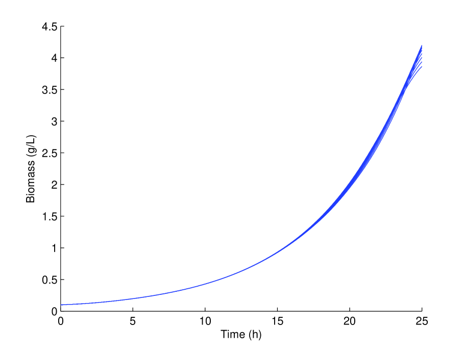
Figure 1: The concentrations of biomass under $u=u^{*}$ and $m_{S}$ varied from 0.8$m_{\mu}$ to 1.2$m_{\mu}$.

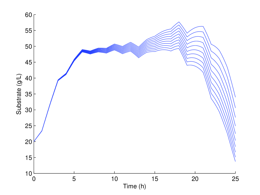
Figure 2: The concentrations of substrate under $u=u^{*}$ and $m_{S}$ varied from 0.8$m_{\mu}$ to 1.2$m_{\mu}$.

To illustrate the superiority of the optimal control strategy obtained from the proposed model, we simulate the system under a constant input $u(t)\equiv 0.01$. The trajectories of biomass and substrate with varied $m_{S}$ under this input strategy are shown in Figs. 3 and 4. A comparison of Fig. 1 and Fig. 3 reveals that, not only the the terminal concentration of biomass under the optimal strategy is significantly higher than that under the constant control input, but also the variation of biomass concentration is much smaller than the constant one. This shows that the system under the optimal control strategy could maintain a good performance even in the “worst” case.

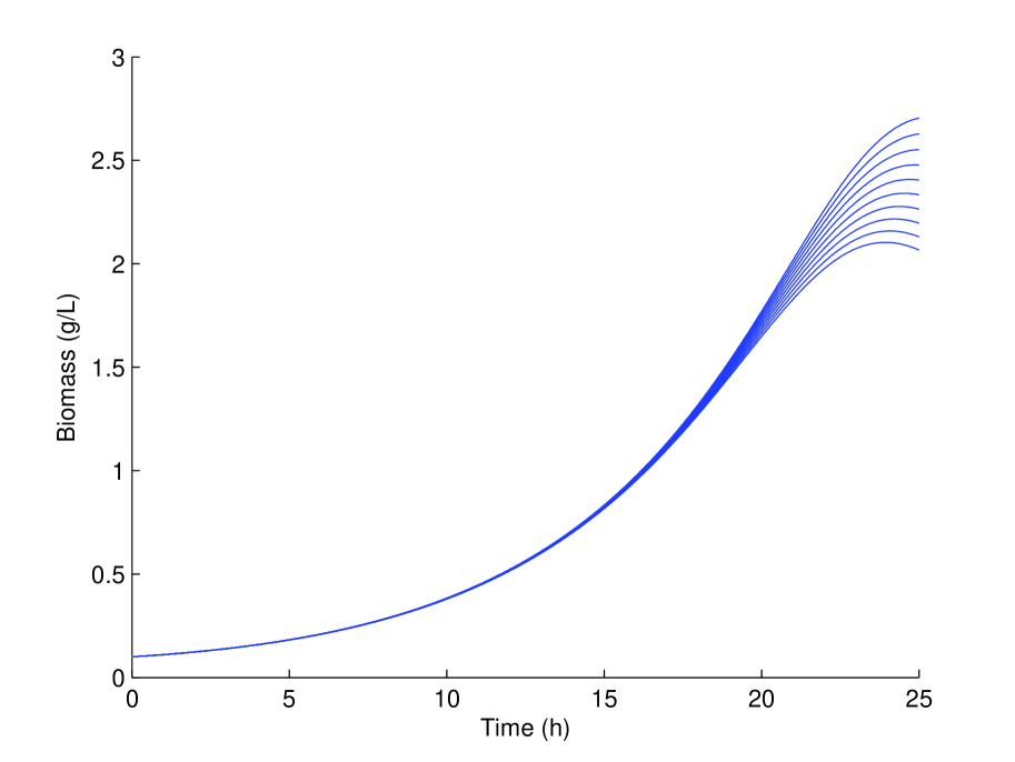
Figure 3: The concentrations of biomass under $u=0.01$ and $m_{S}$ varied from 0.8$m_{\mu}$ to 1.2$m_{\mu}$.

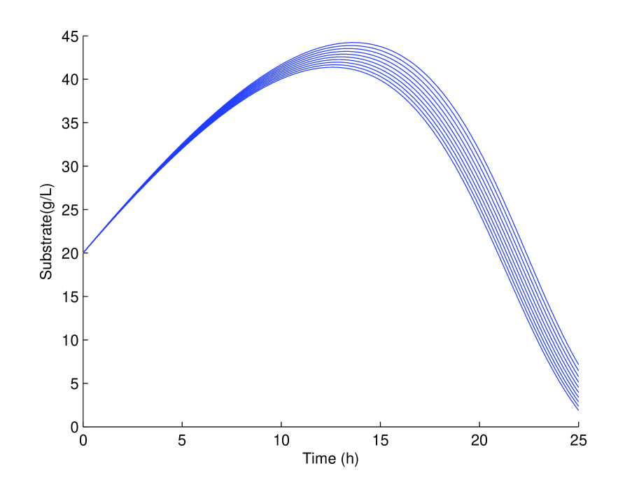
Figure 4: The concentrations of substrate under $u=0.01$ and $m_{S}$ varied from 0.8$m_{\mu}$ to 1.2$m_{\mu}$.

6 Conclusion

This paper introduced an optimal control problem in which both the objective function and the dynamic constraint contain an uncertain parameter. Since the distribution of this uncertain parameter is not exactly known, the objective function is taken as the worst-case expectation over a set of possible distributions of the uncertain parameter. To minimize the worst-case expectation over all possible distributions in an ambiguity set, the stochastic optimal control problem is converted into a finite-dimensional optimization problem via duality and discretization. Necessary conditions of optimality was derived and numerical results for an illustration example are reported. Numerical results in Section 5 show the success of the proposed model in producing an optimal control strategy under which a good performance is achieved. It also ensures that the variation of the performance is small subject to the changes in the value of the uncertain parameter. That is, the system is robust under the optimal control strategy obtained from the proposed model.

The continuation of this work can be divided into two aspects: model aspect and algorithm aspect. The model should take more factors into account. For example, a further study could be on how to introduce proper terminal constraints or path constraints into the model. In the algorithm aspect, the current work transforms the proposed model into a combined optimal control and optimal parameter selection problem and solve it by using nonlinear optimization techniques. However, the special structure of the problem was not taken into detailed investigation. Problem (Dual-DROCP) is linear with respect to the optimization vector $y$ but nonlinear with respect the control $u$. An alternative direction optimization technique could be used to handle these two kinds of optimization variables separately. For example, the control $u$ can be fixed first, and the optimal solution $y_{u}^{*}$ is easily obtained by solving a linear programming problem. Then, the control $u$ is regulated by some nonlinear optimization methods. The procedure is repeated until a satisfactory pair of $(u,y)$ is found. Some stochastic techniques, such as PSO method, could also be combined with the alternative direction optimization technique to regulate the control $u$ in the outer level of the optimization process.

References

• (1) A. L. Soyster. Convex programming with set-inclusive constraints and applications to inexact linear programming. Oper. Res. 1973, 21(5): 1154-1157.
• (2) A. Ben-Tal, L. El Ghaoui, A. Nemirovski. Robust Optimization. Princeton University Press, Princeton, NJ, 2009.
• (3) John R. Birge and F. Louveaux. Introduction to Stochastic Programming. Springer, 2011.
• (4) A. Ruszczynski and A. Shapiro (eds.). Stochastic Programming: Handbook in Operations Research and Management Science. Elsevier Science, Amsterdam, 2003.
• (5) J. Goh, M. Sim. Distributionally robust optimization and its tractable approximations. Oper. Res. 2010, 58(4-part-1): 902-917.
• (6) M. Sim. Distributionally robust optimization: A marriage of robust optimization and stochastic programming. 3rd Nordic Optimization Symposium, March 13-14, 2009, Stockholm, Sweden.
• (7) X. Chen, M. Sim, P. Sun. A robust optimization perspective on stochastic programming. Oper. Res. 2007, 55(6): 1058-1071.
• (8) W. Q. Chen, M. Sim. Goal-driven optimization. Oper. Res. 2009, 57(2): 342-357.
• (9) L El Ghaoui, H. Lebret. Robust solutions to least-squares problems with uncertain data. SIAM J. Matrix Anal. A. 1997, 18(4): 1035-1064.
• (10) D. Erick, and Y. Ye. Distributionally robust optimization under moment uncertainty with application to data-driven problems. Oper. Res. 2010, 58(3): 595-612.
• (11) S Zymler, D Kuhn, B Rustem. Distributionally robust joint chance constraints with second-order moment information. Math. Program. 2013, 137(1-2): 167-198.
• (12) S. Mehrotra, H. Zhang. Models and algorithms for distributionally robust least squares problems. Math. Program. Ser. A. 2013, 1-19.
• (13) Vladimir G. Boltyanski and Alexander S. Poznyak. The Robust Maximum Principle-Theory and Applications. Springer Science & Business Media, 2011.
• (14) E. Polak. Optimization algorithms and consisitent approximations. Springer-Verlag, New York, Inc., 1997.
• (15) A.E. Bryson, Applied optimal control: optimization, estimation and control. CRC Press, 1975.
• (16) K. L. Teo, C. J. Goh. A computational method for combined optimal parameter selection and optimal control problems with general constraints. J. Austral. Math. Soc. Ser. B. 1989(30): 350-364.
• (17) R. Loxton, K. L. Teo, V. Rehbock. Robust Suboptimal Control of Nonlinear Systems. Appl. Math. Comput. 2011(217): 6566-6576
• (18) W.F. Feehery, P.I. Barton. Dynamic optimization with state variable path constraints. Computer Chem. Enging. 1998(22): 1241-1256.
• (19) E. Rosenwasser and R. Yusupov. Sensitivity of Automatic Control Systems. Tom Kurfess(eds). CRC Press, 2000.
• (20) R.C. Loxton, K.L. Teo, V. Rehbock, et al, Optimal control problems with a continuous inequality constraint on the state and the control. Automatica, 2009, 45(10): 2250-2257.
• (21) Jorge Nocedal and Stephen J. Wright. Numerical Optimization. Springer, 2006.
• (22) J. Ye, H. Xu, E. Feng, Z. Xiu. Optimization of a fed-batch bioreactor for 1,3-propanediol production using hybrid nonlinear optimal control. J. Process Contr. 24(2014): 1556-1569.
• (23) A.P. Zeng, W. D. Deckwer. A kinetic model for substrate and energy consumption of microbial growth under substrate-sufficient conditions. Biotechnol. Prog. 11(1995): 71-79.