A minimal model of dynamical phase transition
Abstract
We calculate the large deviation functions characterizing the long-time fluctuations of the occupation of drifted Brownian motion and show that these functions have non-analytic points. This provides the first example of dynamical phase transition that appears in a simple, homogeneous Markov process without an additional low-noise, large-volume or hydrodynamic scaling limit.
Dynamical phase transitions are phase transitions in the fluctuations of physical observables that give rise, similarly to equilibrium phase transitions, to non-analytic points in generalized potentials or large deviation functions characterizing the likelihood of fluctuations. Such transitions are known to arise in many physical systems and scaling limits, including the low-noise limit of diffusion equations modeling noise-perturbed dynamical systems Freidlin and Wentzell (1984); Graham and Tél (1984, 1985); Graham (1989, 1995); Bouchet et al. (2016), thermodynamic-like limits of chaotic systems Beck and Schlögl (1993), and the hydrodynamic limit of interacting particles systems, which corresponds, via the macroscopic fluctuation theory Bertini et al. (2001, 2002, 2007), to a low-noise limit Bertini et al. (2010); Bunin et al. (2012, 2013); Aminov et al. (2014); Baek and Kafri (2015).
Similar transitions also appear in the long-time fluctuations of time-integrated quantities, such as Lyapunov exponents Tailleur and Kurchan (2007); Giardina et al. (2011); Laffargue et al. (2013), dynamical activities Garrahan et al. (2007, 2009); Hedges et al. (2009); Hooyberghs and Vanderzande (2010); Jack and Garrahan (2010); Chandler and Garrahan (2010); Garrahan and Lesanovsky (2010); Garrahan et al. (2011); Genway et al. (2012); Ates et al. (2012); Hickey et al. (2014); Jack and Sollich (2014), currents Rákos and Harris (2008); Gorissen et al. (2009); Gorissen and Vanderzande (2011); Gorissen et al. (2012); Hurtado and Garrido (2011); Espigares et al. (2013); Hurtado et al. (2014); Tsobgni Nyawo and Touchette (2016); Tizón-Escamilla et al. (2016), and the entropy production Gingrich et al. (2014); Mehl et al. (2008); Speck et al. (2012), which now play a central role in studies of nonequilibrium processes. In this case, the large deviation functions are found to be smooth in the long-time limit; singularities start to appear only when a low-noise or a scaling (hydrodynamic, particle or mean-field) limit is taken in addition to the long-time limit 111For quantum systems, this additional limit is often implicit; close inspection shows that it takes either the form of a mean-field limit or a low-noise limit Garrahan and Lesanovsky (2010); Garrahan et al. (2011); Genway et al. (2012); Ates et al. (2012); Hickey et al. (2014)., leading many to believe and claim that these additional limits are necessary for dynamical phase transitions to appear in Markov processes.
The study in Harris and Touchette (2016) of non-homogeneous random walks that are reset in time has just shown, by a mapping to DNA models, that this is not always true – a dynamical phase transition can occur in the long-time limit without a low-noise or scaling limit. Here, we present a simple, minimal model based on a one-dimensional and homogeneous diffusion process that confirms this. The process has no reset and so also shows that random resetting is not needed for such transitions to arise.
The process that we consider is the drifted Brownian motion, defined as
| (1) |
where is the drift, is the noise power, and is the simple, one-dimensional Brownian motion (BM) started at . Physically, may represent the position of a small particle evolving in a fluid moving at slow, constant velocity or in a static fluid but with additional forces (created, e.g., by laser tweezers Ashkin (1997) or an AC trap Cohen and Moerner (2005)) that pull the particle at constant velocity. By analogy with electrical circuits perturbed by Nyquist noise van Zon et al. (2004), can also represent the charge dissipated in a resistor upon the application of a ramped voltage. In both cases, we are interested in the fluctuations of the fraction of time that spends in some interval during a time , which can be expressed as
| (2) |
where is the indicator function equal to if and otherwise. This simple time-integrated quantity is also called the empirical measure of in and is obviously such that , with corresponding to trajectories or paths of that never enter in and to paths that always stay in that interval.
For drifted BM or pure BM (), is very unlikely to stay in any finite interval for a long time, so we must have with probability 1 in the long-time limit . This is confirmed by noticing that the density of gets flatter as time increases, and implies that the probability distribution of concentrates on as .
From the theory of large deviations Ellis (1985); Dembo and Zeitouni (1998); Touchette (2009), we can infer that scales with as
| (3) |
so the concentration of the probability is in fact exponential in time. The function defined by the limit
| (4) |
is called the rate function and characterizes, following (3), the exponentially-small likelihood of observing small and large fluctuations of away from . In practice, this function is most often not determined from the distribution of itself, which is usually unknown or very difficult to obtain, but indirectly from the so-called scaled cumulant generating function (SCGF):
| (5) |
where denotes the expectation and is a real parameter conjugated to the occupation fluctuations. Under some general conditions (see Touchette (2009)), it can indeed be shown that and are related by Legendre-Fenchel transform, so we can obtain the rate function as
| (6) |
This large deviation formalism is the basis of the many recent studies cited before on the fluctuations of the activity, current and entropy production in many-particle Markov dynamics, random walks, and diffusion equations. Our goal now is calculate the SCGF and rate function of for drifted BM and to discuss the appearance of non-analytical points in these functions associated with dynamical phase transitions. The calculations follow the theory explained in Angeletti and Touchette (2016), so we will be brief. To simplify the discussion, we also present the calculations first for and then for .
Pure Brownian motion: The SCGF of additive functionals such as is known to be given by the dominant eigenvalue of the so-called tilted generator Touchette (2009), which corresponds here to
| (7) |
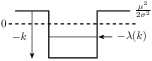
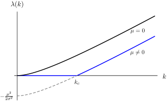
Up to a minus sign, this is just the quantum Hamiltonian associated with a finite well with depth extending from to , so that is simply minus the ground state energy of that well, as illustrated in the inset of Fig. 1. The behavior of the resulting , which depends only on the difference and , is illustrated in the plot of Fig. 1. The main property to notice for our purpose is that is an analytic function in for all , since the ground state energy of the quantum well is itself known to be analytic with the depth of the potential well. This implies that the rate function , shown in Fig. 2, is also analytic for all . Therefore, for pure BM there is no dynamical phase transition in the fluctuations of in the long-time limit.
Drifted Brownian motion: For , the tilted generator becomes
| (8) |
Although this operator is no longer self-adjoint, it is well known that it can be mapped to a Schrödinger-like operator by a unitary “symmetrization” transformation (see Case 2 in Angeletti and Touchette (2016)) which gives here
| (9) |
Consequently, is now determined by (minus) the ground state energy of the quantum well problem, shifted globally by a constant “background” energy (see inset of Fig. 1). This “quantum” eigenvalue, however, cannot give the complete SCGF because it becomes negative for , as shown in Fig. 1. Here, must be positive, since it is convex, , and
| (10) |
To complete the analysis, we have to note that is another possible eigenvalue of . Its corresponding eigenfunction satisfying does not decay to zero at infinity, but is such that as , which is the correct limit of the dominant eigenfunction 222The eigenfunction associated with the quantum eigenvalue does not recover this limit, showing again that this solution does not give the SCGF as .. Taking the maximum between this eigenvalue and the “quantum” eigenvalue above therefore yields
| (11) |
The SCGF is thus a global shift of the solution only when the latter is positive.
With this result, we now see that is non-analytic at the critical point marking the transition from to . In fact, it is clear from Fig. 1 that the first derivative of is discontinuous at this point, which means that the fluctuations of undergo a first-order phase transition when : as crosses , the occupation conjugated to via the Legendre relation Touchette (2009) jumps from 0 (the long-time limit of ) to a strictly positive value , which converges to 1 as . This applies regardless of the sign of since the global shift creating the non-analytic point is even in .
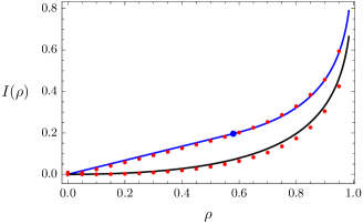
The effect of this transition on the rate function is shown in Fig. 2. The plateau and non-differentiable point of give rise, by the Legendre-Fenchel transform (6), to a linear branch with slope which extends from (so the minimum of is actually a corner) to the critical occupation . Beyond this point, is simply the rate function obtained for shifted by the background . In the limit , both and the shift go to , thereby recovering the rate function of pure BM. This is confirmed in Fig. 2 by numerical results obtained by direct Monte Carlo sampling of 333Simulations were done by sampling trajectories of BM and drifted BM, integrated using a Euler scheme with and . The rate function is obtained by applying (4) without the limit and by shifting the minimal point, corresponding to the mean, at the origin., which also confirm our result for the SCGF.
The linear branch is reminiscent of “coexisting phases” observed in equilibrium first-order phase transitions (e.g., in the phase separation region of the liquid-vapor transition of water) and implies in our context that the fluctuations of are exponential in for . This region of fluctuations seems to be determined by paths of the drifted BM that reach a given occupation by “controlling” their final positions , as observed in Speck et al. (2012); Chetrite and Touchette (2015a); Szavits-Nossan and Evans (2015). Beyond , the probability of is not exponential, since is no longer linear. In this region of large occupations, fluctuations of are created by paths which stay in for a long time and which are therefore not affected by the drift. The probability of seeing such paths in drifted BM compared to pure BM can be computed using Girsanov’s formula Grigoriu (2002): it leads to an extra dominant factor as , which explains the constant shift between the rate functions of drifted and pure BM.
We will provide a more detailed account of these two fluctuation regimes, together with the full solution of the dominant eigenfunction , which shows a delocalization transition, in a future publication 444P. Tsobgni Nyawo, H. Touchette, in preparation, 2016. based on the recently-developed theory of Markov processes conditioned on large deviations Chetrite and Touchette (2013, 2015a, 2015b). At this point, the analytical calculation of is enough to show that the occupation fluctuations of drifted BM undergo a first-order dynamical phase transition, which is confirmed by numerical simulations. The transition does not involve a low-noise or large-system limit and also appears without broken ergodicity Dinwoodie (1993) or long-range (non-Markovian) correlations Cavallaro et al. (2015).
This result and the simplicity of the model underlying it raise many interesting questions about the nature and conditions needed for the appearance of dynamical phase transitions. We suggest to conclude three particular questions that we see as important for future studies:
1. Can conditions known for equilibrium phase transitions (related, e.g., to dimensionality and the range of interactions) be reformulated for dynamical phase transitions? Some basic ideas related to that question can be found in Rákos and Harris (2008). One way to map drifted BM or any other continuous-time processes to an “equilibrium” particle model is to view time as an extra space dimension and to relate the SCGF to a partition function.
2. What is the relation between the transition observed here and those observed in the weak-noise limit Graham and Tél (1984, 1985); Graham (1989, 1995), which have been re-discovered recently under the name “Lagrangian phase transitions” Bertini et al. (2010)? This should be answered by comparing the variational representations of the SCGF and the rate function obtained with and without the low-noise limit Chetrite and Touchette (2015b).
3. Does the phase transition of drifted BM disappear if we “compactify” this process on a ring or a closed interval? In other words, is the phase transition only a result of drifted BM evolving on an “infinite” state space (the real line)? It is commonly believed that the SCGF of compact, irreducible Markov processes must be analytic, but to our knowledge this has yet to be proved in general beyond the cases of finite Markov jump processes and Markov chains. Moreover, although is unbounded, the occupation observable for which the phase transition occurs is bounded. Finally, there are many models that evolve in infinite space and yet do not give rise to phase transitions (e.g., pure BM), so the issue of infinite versus finite spaces is a subtle one.
Acknowledgements.
We thank Cesare Nardini, Frédéric van Wijland, and Raphaël Chetrite for useful comments. P.T.N. is supported by a DAAD Scholarship. H.T. is supported by the National Research Foundation of South Africa (Grants no. 90322 and 96199) and Stellenbosch University (Project Funding for New Appointee).References
- Freidlin and Wentzell (1984) M. I. Freidlin and A. D. Wentzell, Random Perturbations of Dynamical Systems, Grundlehren der Mathematischen Wissenschaften, Vol. 260 (Springer, New York, 1984).
- Graham and Tél (1984) R. Graham and T. Tél, “On the weak-noise limit of Fokker-Planck models,” J. Stat. Phys. 35, 729–748 (1984).
- Graham and Tél (1985) R. Graham and T. Tél, “Weak-noise limit of Fokker-Planck models and nondifferentiable potentials for dissipative dynamical systems,” Phys. Rev. A 31, 1109–1122 (1985).
- Graham (1989) R. Graham, “Macroscopic potentials, bifurcations and noise in dissipative systems,” in Noise in Nonlinear Dynamical Systems, Vol. 1, edited by F. Moss and P. V. E. McClintock (Cambridge University Press, Cambridge, 1989) pp. 225–278.
- Graham (1995) R. Graham, “Fluctuations in the steady state,” in 25 Years of Non-Equilibrium Statistical Mechanics, edited by J. J. Brey, J. Marro, J. M. Rubí, and M. San Miguel (Springer, New York, 1995) pp. 125–134.
- Bouchet et al. (2016) F. Bouchet, K. Gawedzki, and C. Nardini, “Perturbative calculation of quasi-potential in non-equilibrium diffusions: A mean-field example,” J. Stat. Phys. 163, 1157–1210 (2016).
- Beck and Schlögl (1993) C. Beck and F. Schlögl, Thermodynamics of Chaotic Systems: An Introduction (Cambridge University Press, Cambridge, 1993).
- Bertini et al. (2001) L. Bertini, A. De Sole, D. Gabrielli, G. Jona-Lasinio, and C. Landim, “Fluctuations in stationary nonequilibrium states of irreversible processes,” Phys. Rev. Lett. 87, 040601 (2001).
- Bertini et al. (2002) L. Bertini, A. De Sole, D. Gabrielli, G. Jona-Lasinio, and C. Landim, “Macroscopic fluctuation theory for stationary non-equilibrium states,” J. Stat. Phys. 107, 635–675 (2002).
- Bertini et al. (2007) L. Bertini, A. De Sole, D. Gabrielli, G. Jona-Lasinio, and C. Landim, “Stochastic interacting particle systems out of equilibrium,” J. Stat. Mech. 2007, P07014 (2007).
- Bertini et al. (2010) L. Bertini, A. De Sole, D. Gabrielli, G. Jona-Lasinio, and C. Landim, “Lagrangian phase transitions in nonequilibrium thermodynamic systems,” J. Stat. Mech. 2010, L11001 (2010).
- Bunin et al. (2012) G. Bunin, Y. Kafri, and D. Podolsky, “Non-differentiable large-deviation functionals in boundary-driven diffusive systems,” J. Stat. Mech. 2012, L10001 (2012).
- Bunin et al. (2013) G. Bunin, Y. Kafri, and D. Podolsky, “Cusp singularities in boundary-driven diffusive systems,” J. Stat. Phys. 152, 112–135 (2013).
- Aminov et al. (2014) A. Aminov, G. Bunin, and Y. Kafri, “Singularities in large deviation functionals of bulk-driven transport models,” J. Stat. Mech. 2014, P08017 (2014).
- Baek and Kafri (2015) Y. Baek and Y. Kafri, “Singularities in large deviation functions,” J. Stat. Mech. 2015, P08026 (2015).
- Tailleur and Kurchan (2007) J. Tailleur and J. Kurchan, “Probing rare physical trajectories with Lyapunov weighted dynamics,” Nat. Phys. 3, 203–207 (2007).
- Giardina et al. (2011) C. Giardina, J. Kurchan, V. Lecomte, and J. Tailleur, “Simulating rare events in dynamical processes,” J. Stat. Phys. 145, 787–811 (2011).
- Laffargue et al. (2013) T. Laffargue, K.-D. Nguyen Thu Lam, J. Kurchan, and J. Tailleur, “Large deviations of Lyapunov exponents,” J. Phys. A: Math. Theor. 46, 254002 (2013).
- Garrahan et al. (2007) J. P. Garrahan, R. L. Jack, V. Lecomte, E. Pitard, K. van Duijvendijk, and F. van Wijland, “Dynamical first-order phase transition in kinetically constrained models of glasses,” Phys. Rev. Lett. 98, 195702 (2007).
- Garrahan et al. (2009) J. P. Garrahan, R. L. Jack, V. Lecomte, E. Pitard, K. van Duijvendijk, and F. van Wijland, “First-order dynamical phase transition in models of glasses: An approach based on ensembles of histories,” J. Phys. A: Math. Theor. 42, 075007 (2009).
- Hedges et al. (2009) L. O. Hedges, R. L. Jack, J. P. Garrahan, and D. Chandler, “Dynamic order-disorder in atomistic models of structural glass formers,” Science 323, 1309–1313 (2009).
- Hooyberghs and Vanderzande (2010) J. Hooyberghs and C. Vanderzande, “Thermodynamics of histories for the one-dimensional contact process,” J. Stat. Mech. 2010, P02017 (2010).
- Jack and Garrahan (2010) R. L. Jack and J. P. Garrahan, “Metastable states and space-time phase transitions in a spin-glass model,” Phys. Rev. E 81, 011111 (2010).
- Chandler and Garrahan (2010) D. Chandler and J. P. Garrahan, “Dynamics on the way to forming glass: Bubbles in space-time,” Ann. Rev. Chem. Phys. 61, 191–217 (2010).
- Garrahan and Lesanovsky (2010) J. P. Garrahan and I. Lesanovsky, “Thermodynamics of quantum jump trajectories,” Phys. Rev. Lett. 104, 160601 (2010).
- Garrahan et al. (2011) J. P. Garrahan, A. D. Armour, and I. Lesanovsky, “Quantum trajectory phase transitions in the micromaser,” Phys. Rev. E 84, 021115 (2011).
- Genway et al. (2012) S. Genway, J. P. Garrahan, I. Lesanovsky, and A. D. Armour, “Phase transitions in trajectories of a superconducting single-electron transistor coupled to a resonator,” Phys. Rev. E 85, 051122 (2012).
- Ates et al. (2012) C. Ates, B. Olmos, J. P. Garrahan, and I. Lesanovsky, “Dynamical phases and intermittency of the dissipative quantum Ising model,” Phys. Rev. A 85, 043620 (2012).
- Hickey et al. (2014) J. M. Hickey, C. Flindt, and J. P. Garrahan, “Intermittency and dynamical Lee-Yang zeros of open quantum systems,” Phys. Rev. E 90, 062128 (2014).
- Jack and Sollich (2014) R. L. Jack and P. Sollich, “Large deviations of the dynamical activity in the East model: Analysing structure in biased trajectories,” J. Phys. A: Math. Theor. 47, 015003 (2014).
- Rákos and Harris (2008) A. Rákos and R. J. Harris, “On the range of validity of the fluctuation theorem for stochastic Markovian dynamics,” J. Stat. Mech. 2008, P05005 (2008).
- Gorissen et al. (2009) M. Gorissen, J. Hooyberghs, and C. Vanderzande, “Density-matrix renormalization-group study of current and activity fluctuations near nonequilibrium phase transitions,” Phys. Rev. E 79, 020101 (2009).
- Gorissen and Vanderzande (2011) M. Gorissen and C. Vanderzande, “Finite size scaling of current fluctuations in the totally asymmetric exclusion process,” J. Phys. A: Math. Theor. 44, 115005 (2011).
- Gorissen et al. (2012) M. Gorissen, A. Lazarescu, K. Mallick, and C. Vanderzande, “Exact current statistics of the asymmetric simple exclusion process with open boundaries,” Phys. Rev. Lett. 109, 170601 (2012).
- Hurtado and Garrido (2011) P. I. Hurtado and P. L. Garrido, “Spontaneous symmetry breaking at the fluctuating level,” Phys. Rev. Lett. 107, 180601 (2011).
- Espigares et al. (2013) C. P. Espigares, P. L. Garrido, and P. I. Hurtado, “Dynamical phase transition for current statistics in a simple driven diffusive system,” Phys. Rev. E 87, 032115 (2013).
- Hurtado et al. (2014) P. I. Hurtado, C. P. Espigares, J. J. del Pozo, and P. L. Garrido, “Thermodynamics of currents in nonequilibrium diffusive systems: Theory and simulation,” J. Stat. Phys. 154, 214–264 (2014).
- Tsobgni Nyawo and Touchette (2016) P. Tsobgni Nyawo and H. Touchette, “Large deviations of the current for driven periodic diffusions,” Phys. Rev. E 94, 032101 (2016).
- Tizón-Escamilla et al. (2016) N. Tizón-Escamilla, C. Pérez-Espigares, P. L. Garrido, and P. I. Hurtado, “Order and symmetry-breaking in the fluctuations of driven systems,” (2016), arxiv:1606.07507 .
- Gingrich et al. (2014) T. R. Gingrich, S. Vaikuntanathan, and P. L. Geissler, “Heterogeneity-induced large deviations in activity and (in some cases) entropy production,” Phys. Rev. E 90, 042123 (2014).
- Mehl et al. (2008) J. Mehl, T. Speck, and U. Seifert, “Large deviation function for entropy production in driven one-dimensional systems,” Phys. Rev. E 78, 011123 (2008).
- Speck et al. (2012) T. Speck, A. Engel, and U. Seifert, “The large deviation function for entropy production: The optimal trajectory and the role of fluctuations,” J. Stat. Mech. 2012, P12001 (2012).
- Note (1) For quantum systems, this additional limit is often implicit; close inspection shows that it takes either the form of a mean-field limit or a low-noise limit Garrahan and Lesanovsky (2010); Garrahan et al. (2011); Genway et al. (2012); Ates et al. (2012); Hickey et al. (2014).
- Harris and Touchette (2016) R. J. Harris and H. Touchette, “Phase transitions in large deviations of reset processes,” J. Phys. A: Math. Theor. (2016), arxiv:1610.08842 .
- Ashkin (1997) A. Ashkin, “Optical trapping and manipulation of neutral particles using lasers,” Proc. Nat. Acad. Sci. (USA) 94, 4853–4860 (1997).
- Cohen and Moerner (2005) A. E. Cohen and W. E. Moerner, “Method for trapping and manipulating nanoscale objects in solution,” App. Phys. Lett. 86, 093109 (2005).
- van Zon et al. (2004) R. van Zon, S. Ciliberto, and E. G. D. Cohen, “Power and heat fluctuation theorems for electric circuits,” Phys. Rev. Lett. 92, 130601 (2004).
- Ellis (1985) R. S. Ellis, Entropy, Large Deviations, and Statistical Mechanics (Springer, New York, 1985).
- Dembo and Zeitouni (1998) A. Dembo and O. Zeitouni, Large Deviations Techniques and Applications, 2nd ed. (Springer, New York, 1998).
- Touchette (2009) H. Touchette, “The large deviation approach to statistical mechanics,” Phys. Rep. 478, 1–69 (2009).
- Angeletti and Touchette (2016) F. Angeletti and H. Touchette, “Diffusions conditioned on occupation measures,” J. Math. Phys. 53, 023303 (2016).
- Note (2) The eigenfunction associated with the quantum eigenvalue does not recover this limit, showing again that this solution does not give the SCGF as .
- Note (3) Simulations were done by sampling trajectories of BM and drifted BM, integrated using a Euler scheme with and . The rate function is obtained by applying (4) without the limit and by shifting the minimal point, corresponding to the mean, at the origin.
- Chetrite and Touchette (2015a) R. Chetrite and H. Touchette, “Nonequilibrium Markov processes conditioned on large deviations,” Ann. Inst. Poincaré A 16, 2005–2057 (2015a).
- Szavits-Nossan and Evans (2015) J. Szavits-Nossan and M. R. Evans, “Inequivalence of nonequilibrium path ensembles: The example of stochastic bridges,” J. Stat. Mech. , P12008 (2015), 1508.04969 .
- Grigoriu (2002) M. Grigoriu, Stochastic Calculus: Applications in Science and Engineering (Birkhäuser, Boston, 2002).
- Note (4) P. Tsobgni Nyawo, H. Touchette, in preparation, 2016.
- Chetrite and Touchette (2013) R. Chetrite and H. Touchette, “Nonequilibrium microcanonical and canonical ensembles and their equivalence,” Phys. Rev. Lett. 111, 120601 (2013).
- Chetrite and Touchette (2015b) R. Chetrite and H. Touchette, “Variational and optimal control representations of conditioned and driven processes,” J. Stat. Mech. 2015, P12001 (2015b).
- Dinwoodie (1993) I. H. Dinwoodie, “Identifying a large deviation rate function,” Ann. Prob. 21, 216–231 (1993).
- Cavallaro et al. (2015) M. Cavallaro, R. J. Mondragón, and R. J. Harris, “Temporally correlated zero-range process with open boundaries: Steady state and fluctuations,” Phys. Rev. E 92, 022137 (2015).