Conditioned Langevin Dynamics enables efficient sampling of transition paths

Abstract

We propose a novel stochastic method to generate Brownian paths conditioned to start at an initial point and end at a given final point during a fixed time $t_{f}$ under a given potential $U(x)$. These paths are sampled with a probability given by the overdamped Langevin dynamics. We show that these paths can be exactly generated by a local Stochastic Partial Differential Equation (SPDE). This equation cannot be solved in general. We present several approximations that are valid either in the low temperature regime or in the presence of barrier crossing. We show that this method warrants the generation of statistically independent transition paths. It is computationally very efficient. We illustrate the method on the two dimensional Mueller potential as well as on the Mexican hat potential.

Pasteur] Unité de Dynamique Structurale des Macromolécules, URA 3528 du CNRS, Institut Pasteur, 75015 Paris, France Davis] Department of Computer Sciences and Genome Center, University of California, Davis, CA 95616, USA CEA] Institut de Physique Théorique, CEA, IPhT, CNRS, URA2306, F-91191 Gif-sur-Yvette, France [BCSRC] Beijing Computational Science Research Center, No.3 HeQing Road, Haidian District, Beijing, 100084, China

1 Introduction

Chemical and biological are controlled by dynamics. Indeed, it is the ability of molecules to change conformations that leads to their activity. Observing experimentally or predicting functional conformational changes is however a very difficult problem. At the core of this problem is the fact that a transition between two conformations of a molecule is a rare event compared to the time scale of the internal dynamics of the molecule. This event is a consequence of random perturbations in the structure of the molecule, drawing its energy from the surrounding heat bath; it is rare whenever the energy barrier that needs to be crossed is high compared to $k_{B}T$. The transition state theory (TST) offers a framework for studying such rare events ^{1, 2}. The main idea of the TST is that the transition state is a saddle point of the energy surface for the molecule of interest. In many cases, the most probable transition path is then simply the minimum energy path (MEP) along that energy surface. The TST however is limited to situations in which the potential energy surface is rather smooth; it also assumes that every crossing of the energy barrier through the transition state gives rise to a successful reaction. For systems with a rugged potential energy landscape, or when entropic effects matter, the saddle points do not necessarily play the role of transition states ³.

To alleviate the shortcomings of the TST, Vanden Eijden and colleagues proposed an alternate view of transitions, the Transition Path Theory (TPT) ^{4, 3, 5}. At zero temperature the TPT is deemed exact. In principle, it eliminates the need for sampling the transition path ensemble. It also provides a framework for finding the shortest, or most probable transition path between two conformations of a molecule. As such, it has served as a touchstone for the development of many path finding algorithms. Some of those were developed for finding the Minimum Energy Path on the energy surface for a molecule, such as morphing techniques ^{6, 7}, gradient descent methods ^{8, 9, 10, 11}, the nudged elastic band method (NEB) ^{12, 13, 14} and the string method ^{15, 16, 17, 18, 19, 20}. Other algorithms are concerned with either finding the Minimum Free Energy Path on the free energy surface for the molecule,^{21, 22, 23, 24}. or finding the path that minimizes a functional, as implemented in the Minimum Action Path methods ^{25, 26, 27, 28, 29, 30, 31}. This list is not a comprehensive coverage of all existing techniques for finding transition paths, as this is a very active area of research with many techniques proposed every year.

Due to the inherent fluctuations underlying the transition phenomenon there are many ways however in which a transition can take place. The methods described above usually generate one path along this transition, the most “probable” one, where probable refers to minimum energy, free energy, or an action. Path sampling methods expand upon this view by using this path as a seed to generate a Monte Carlo random walk in the path space of the transition trajectories, and thus generate an approximation of the ensemble of all possible transition paths ^{32, 33}. All the relevant kinetic and thermodynamic information related to the transition can then be extracted from the ensemble, such as the reaction mechanism, the transition states, and the rate constants. The main drawback of these methods however is that they are very time consuming and therefore limited to small systems. In addition, they generate highly correlated trajectories in which case the space of sampled trajectories depends strongly on the initial path.

In parallel to path sampling methods, much effort has recently been dedicated to the development and analysis of Markov State Models (MSMs) ^{34, 35, 36}. MSMs aim at coarse-graining the dynamics of the molecular system via mapping it onto a continuous-time Markov jump process, that is, a process whose evolution involves jumps between discretized states representing typical conformations of the original system. Much of the recent work focuses on generating those conformations and the dynamics between them, usually using molecular dynamics simulations. To this day, MSMs remain computationally intensive methods.

In this paper we are concerned with the problem of path sampling. Following preliminary work by one of us ³⁷, we propose a novel method for generating paths using a Stochastic Partial Differential Equation (SPDE). This equation cannot be solved in general but we were able to find approximations that are valid for different regimes for the dynamics of the system.

The paper is organized as follows. In the next section, we derive the SPDE and describe the different approximations we have implemented to solve this equation. In the following section, we show applications to two well-studied 2D problems. Finally, we conclude the paper with a discussion of the extension of the method to study transition pathways for bio-molecular systems.

2 Theory

2.1 Derivation of the bridge equation

We assume that the system is driven by a force $F(x,t)$ and is subject to stochastic dynamics in the form of an overdamped Langevin equation.

For the sake of simplicity, we illustrate the method on a one-dimensional system, the generalization to higher dimensions or larger number of degrees of freedom being straightforward. We follow closely the presentation given in Ref. ³⁷.

The overdamped Langevin equation reads

$$\frac{dx}{dt}=\frac{1}{\gamma}F(x(t),t)+\sqrt{\frac{2k_{B}T}{\gamma}}\eta(t)$$ (1)

where $x(t)$ is the position of the particle at time $t$, driven by the force $F(x,t)$, $\gamma$ is the friction coefficient, related to the diffusion coefficient $D$ through the Einstein relation $D=k_{B}T/\gamma$, where $k_{B}$ is the Boltzmann constant and $T$ the temperature of the heat bath. In addition, $\eta(t)$ is a Gaussian white noise with moments given by

$$\langle\eta(t)\rangle=0$$ (2)

$$\langle\eta(t)\eta(t^{\prime})\rangle=\delta(t-t^{\prime})$$ (3)

The probability distribution $P(x,t)$ for the particle to be at point $x$ at time $t$ satisfies a Fokker-Planck equation ^{38, 39},

$$\frac{\partial P}{\partial t}=D\frac{\partial}{\partial x}\left(\frac{\partial P}{\partial x}-\beta FP\right)$$ (4)

where $\beta=1/k_{B}T$ is the inverse temperature. This equation is to be supplemented by the initial condition $P(x,0)=\delta(x-x_{0})$, where the particle is assumed to be at $x_{0}$ at time $t=0$. To emphasize this initial condition, we will often use the notation $P(x,t)=P(x,t|x_{0},0)$.

We now study the probability over all paths starting at $x_{0}$ at time $0$ and conditioned to end at a given point $x_{f}$ at time $t_{f}$, to find the particle at point $x$ at time $t\in[0,t_{f}]$. This probability can be written as

$$\mathcal{P}(x,t)=\frac{1}{P(x_{f},t_{f}|x_{0},0)}Q(x,t)P(x,t)$$

where we use the notation

$$P(x,t)=P(x,t|x_{0},0)$$

$$Q(x,t)=P(x_{f},t_{f}|x,t)$$

Indeed, the probability for a path starting from $(x_{0},0)$ and ending at $(x_{f},t_{f})$ to go through $x$ at time $t$ is the product of the probability $P(x,t|x_{0},0)$ to start at $(x_{0},0)$ and to end at $(x,t)$ by the probability $P(x_{f},t_{f}|x,t)$ to start at $(x,t)$ and to end at $(x_{f},t_{f})$.

The equation satisfied by $P$ is the Fokker-Planck equation mentioned above (4), whereas that for $Q$ is the so-called reverse or adjoint Fokker-Planck equation ^{38, 39} given by

$$\frac{\partial Q}{\partial t}=-D\frac{\partial^{2}Q}{\partial x^{2}}-D\beta F\frac{\partial Q}{\partial x}$$ (5)

It can be easily checked that the conditional probability $\mathcal{P}(x,t)$ satisfies a new Fokker-Planck equation

$$\frac{\partial\mathcal{P}}{\partial t}=D\frac{\partial}{\partial x}\left(\frac{\partial\mathcal{P}}{\partial x}-\left(\beta F+2\frac{\partial\ln Q}{\partial x}\right)\mathcal{P}\right)$$

Comparing this equation with the initial Fokker-Planck (4) and Langevin (1) equations, one sees that it can be obtained from a Langevin equation with an additional potential force

$$\frac{dx}{dt}=\frac{1}{\gamma}F+2D\frac{\partial\ln Q}{\partial x}+\sqrt{\frac{2k_{B}T}{\gamma}}\eta(t)$$ (6)

This equation has been previously obtained using the Doob transform ^{40, 41} in the probability literature and provides a simple recipe to construct a generalized bridge. It generates Brownian paths, starting at $(x_{0},0)$ conditioned to end at $(x_{f},t_{f})$, with unbiased statistics. It is the additional term $2D\frac{\partial\ln Q}{\partial x}$ in the Langevin equation that guarantees that the trajectories starting at $(x_{0},0)$ and ending at $(x_{f},t_{f})$ are statistically unbiased. This equation can be easily generalized to any number of degrees of freedom.

In the following, we will specialize to the case where the force $F$ is derived from a potential $U(x)$. The bridge equation becomes

$$\frac{dx}{dt}=-\frac{1}{\gamma}\frac{\partial U}{\partial x}+2D\frac{\partial\ln Q}{\partial x}+\sqrt{\frac{2k_{B}T}{\gamma}}\eta(t)$$ (7)

In that case, the Fokker-Planck equation corresponding to this modified Langevin equation can be recast into an imaginary time Schrödinger equation ³⁷, and the probability distribution function $P$ can be written as

$$Q(x,t)=P(x_{f},t_{f}|x,t)=e^{-\beta(U(x_{f})-U(x))/2}\langle x_{f}|e^{-H(t_{f}-t)}|x\rangle$$ (8)

where $H$ is a ”quantum Hamiltonian” defined by

$$H=-D\frac{\partial^{2}}{\partial x^{2}}+D\frac{\beta^{2}}{4}V(x)$$ (9)

and the potential $V$ by

$$V=\left(\frac{\partial U}{\partial x}\right)^{2}-2k_{B}T\frac{\partial^{2}U}{\partial x^{2}}$$ (10)

We denote by $M$ the matrix element of the Euclidian Schrödinger evolution operator

$$M(x,t)=\langle x_{f}|e^{-H(t_{f}-t)}|x\rangle$$ (11)

Using eq.(8) for $Q$, one can write equation (7) as

$$\frac{dx}{dt}=2\frac{k_{B}T}{\gamma}\frac{\partial}{\partial x}\ln M(x,t)+\sqrt{\frac{2k_{B}T}{\gamma}}\eta(t)$$ (12)

We see on the above form that when $t\to t_{f}$, the matrix element $M(x,t)$ converges to $\delta(x_{f}-x)$, and it is this singular attractive potential which drives all the paths to $x_{f}$ at time $t_{f}$.

2.2 Transition paths

The bridge equations (7) or (12) can be solved exactly in a certain number of cases ⁴². However in general, for systems with many degrees of freedom, the functions $Q(x,t)$ or $M(x,t)$ cannot be computed exactly and one has to resort to some approximations. In the following, we will be mostly interested in problems of energy or entropy barrier crossing, which are of utmost importance in many chemical, biochemical, or biological reactions.

The matrix element $M(x,t)$ can be written as a Feynman path integral

$$M(x,t)=\int_{x(t)=x}^{x(t_{f})=x_{f}}\mathcal{D}x\>\exp\left(-\int_{t}^{t_{f}}d\tau\left(\frac{1}{4D}\left(\frac{dx}{d\tau}\right)^{2}+\frac{D\beta^{2}}{4}V(x(\tau))\right)\right)$$ (13)

The free case is defined as

$$M_{0}(x,t) = P_{0}(x_{f},t_{f}|x,t)$$ (14)

$$= \int_{x(t)=x}^{x(t_{f})=x_{f}}\mathcal{D}x\>\exp\left(-\int_{t}^{t_{f}}d\tau\left(\frac{1}{4D}\left(\frac{dx}{d\tau}\right)^{2}\right)\right)$$

$$= \left(\frac{1}{4\pi D(t_{f}-t)}\right)^{1/2}e^{-\frac{\left(x_{f}-x\right)^{2}}{4D(t_{f}-t)}}$$

where $P_{0}$ is the probability distribution for a free particle.

Equation (13) can be rewritten as

$$M(x,t)=M_{0}(x,t)\langle\exp\left(-\frac{D\beta^{2}}{4}\int_{t}^{t_{f}}d\tau V(x(\tau))\right)\rangle_{0}$$

where the expression $\langle...\rangle_{0}$ denotes the expectation value with the Brownian measure $P_{0}$.

The convexity of the exponential function implies the Jensen inequality ⁴³, which states that for any operator $A$ and any probability measure, one has

$$\langle e^{-A}\rangle\geq e^{-\langle A\rangle}$$ (15)

Equality occurs when the probability is a $\delta-$function; it is thus a good approximation when the operator $A$ has small fluctuations.Taking $A$ to be

$$A=\frac{D\beta^{2}}{4}\int_{t}^{t_{f}}d\tau V(x(\tau))$$ (16)

we have

$$M(x,t)\simeq M_{0}(x,t)\exp\left(-\frac{D\beta^{2}}{4}\int_{t}^{t_{f}}d\tau\langle V(x(\tau))\rangle_{0}\right)$$ (17)

Using the expression

$$\langle V(x(\tau))\rangle_{0}=\frac{1}{M_{0}(x,t)}\int dzP_{0}(x_{f},t_{f}|z,\tau)V(z)P_{0}(z,\tau|x,t),$$

after some calculations, we obtain

$$\langle V(x(\tau))\rangle_{0}=\left(\frac{\theta_{1}+\theta_{2}}{4\pi D\theta_{1}\theta_{2}}\right)^{1/2}\int dz\exp\left(-\frac{\theta_{1}+\theta_{2}}{4D\theta_{1}\theta_{2}}\left(z-\frac{x_{f}\theta_{2}+x\theta_{1}}{\theta_{1}+\theta_{2}}\right)^{2}\right)V(z)$$

where

$$\theta_{1}=t_{f}-\tau,\;\theta_{2}=\tau-t$$

After a change of variable, this expression becomes

$$\langle V(x(\tau))\rangle_{0}=\int\frac{dz}{\left(2\pi\right)^{1/2}}\exp\left(-\frac{z^{2}}{2}\right)V\left(X+\sqrt{\frac{2D\theta_{1}\theta_{2}}{\theta_{1}+\theta_{2}}}z\right)$$

where

$$X=\frac{x_{f}\theta_{2}+x\theta_{1}}{\theta_{1}+\theta_{2}}$$

and the constrained Langevin equation (12) becomes

$$\frac{dx}{dt} = \frac{x_{f}-x}{t_{f}-t}$$ (18)

$$- \frac{(D\beta)^{2}}{2}\int_{t}^{t_{f}}d\tau\left(\frac{t_{f}-\tau}{t_{f}-t}\right)\int\frac{dz}{\left(2\pi\right)^{1/2}}\exp\left(-\frac{z^{2}}{2}\right)\frac{\partial}{\partial X}V\left(X+\sqrt{\frac{2D(t_{f}-\tau)(\tau-t)}{(t_{f}-t)}}z\right)$$

$$+ \sqrt{\frac{2k_{B}T}{\gamma}}\eta(t)$$

or, after the change of variable $u=\frac{\tau-t}{t_{f}-t}=\frac{\theta_{2}}{\theta_{1}+\theta_{2}}$,

$$\frac{dx}{dt} = \frac{x_{f}-x}{t_{f}-t}$$ (19)

$$- \frac{(D\beta)^{2}}{2}(t_{f}-t)\int_{0}^{1}du(1-u)\int\frac{dz}{\left(2\pi\right)^{1/2}}\exp\left(-\frac{z^{2}}{2}\right)\frac{\partial}{\partial X}V\left(X+\sqrt{2D(t_{f}-t)u(1-u)}z\right)$$

$$+ \sqrt{\frac{2k_{B}T}{\gamma}}\eta(t)$$

where

$$X=x_{f}u+x(1-u)$$ (20)

Integration by part with respect to $z$ yields the equivalent form

$$\frac{dx}{dt} = \frac{x_{f}-x}{t_{f}-t}$$ (21)

$$- \left(\frac{D}{2}\right)^{3/2}\beta^{2}\sqrt{t_{f}-t}\int_{0}^{1}du\sqrt{\frac{1-u}{u}}\int\frac{dz}{\left(2\pi\right)^{1/2}}\exp\left(-\frac{z^{2}}{2}\right)zV\left(X+\sqrt{2D(t_{f}-t)u(1-u)}z\right)$$

$$+ \sqrt{\frac{2k_{B}T}{\gamma}}\eta(t)$$

which does not require the cumbersome evaluation of $\partial V/\partial X$. These forms require an integration over the Gaussian variable $z$ which can be performed by sampling this variable

$$\int\frac{dz}{\left(2\pi\right)^{1/2}}\exp\left(-\frac{z^{2}}{2}\right)F(z)\simeq\frac{1}{M}\sum_{i}F(z_{i})$$

where the $M$ variables $z_{i}$ are Gaussian variables (with zero average and unit variance).

However, as we have seen, the approximation (17) is valid if the exponent $A$ does not fluctuate too much over the trajectories relevant to the transition. There are two cases when this approximation can be further simplified and where the $z$-integral can be avoided:

1. Low temperature

   In that case, since $D=k_{B}T/\gamma$, diffusion is small, thus $V$ can be approximated as $(\frac{\partial U}{\partial x})^{2}$. In addition, the term $\sqrt{2D(t_{f}-t)u(1-u)}z$ in (19) is small compared to $X$ and can be neglected. Equation (18) can be simplified to

   $$\frac{dx}{dt}=\frac{x_{f}-x}{t_{f}-t}-\frac{(D\beta)^{2}}{2}(t_{f}-t)\int_{0}^{1}du(1-u)\frac{\partial}{\partial X}\left(\frac{\partial}{\partial X}U\left(X\right)\right)^{2}+\sqrt{\frac{2k_{B}T}{\gamma}}\eta(t)$$ (22)

2. Barrier crossing

   According to Kramers theory, the total transition time $\tau_{K}$ (waiting + crossing) scales like the exponential of the barrier height $\Delta E^{*}$ while it has been shown that the crossing time (Transition Path Time) $\tau_{c}$ scales like the logarithm of the barrier $\Delta E^{*}$ ^{44, 45, 46}. We have thus $\tau_{c}<<\tau_{K}$.

   As discussed before, the barrier crossing time is very short compared to the Kramers time. Therefore the transition trajectories are very weakly diffusive, and are thus almost ballistic. Consequently, we have $\sqrt{2Dt_{f}}\ll|x_{f}-x_{0}|$ and again we can neglect the $z$ term in $V$. Equation (18) becomes

   $$\frac{dx}{dt}=\frac{x_{f}-x}{t_{f}-t}-\frac{(D\beta)^{2}}{2}(t_{f}-t)\int_{0}^{1}du(1-u)\frac{\partial V(X)}{\partial X}+\sqrt{\frac{2k_{B}T}{\gamma}}\eta(t)$$ (23)

All the equations described above are easily generalized to any number of particles in any dimension, interacting with any many-body potentials. They are integro-differential stochastic Markov equations, as the variable $X$ depends only on the stochastic variable $x(t)$. One can generate many independent trajectories by integrating these equations with different noise histories $\eta(t)$. To test the validity of the main approximation (17), one should compute the variance $(\Delta A)^{2}=\langle A^{2}\rangle-\langle A\rangle^{2}$ of the random variable $A$ in eq.(16) over all the trajectories generated. Computing the correction to the Jensen inequality, it is easily seen that the approximation is reliable provided

$$R=\frac{(\Delta A)^{2}}{2|\langle A\rangle|}<<1$$ (24)

2.3 Simulation Time

For barrier crossing, what simulation time $t_{f}$ should be used? Obviously, for any initial and final state $x_{i}$ and $x_{f}$, there is a set of Langevin trajectories which make the transition in any given time $t_{f}$. If the time $t_{f}$ is very short compared to the typical time scales of large motions of the system, there is a small number of such trajectories, since they require a very specific noise history. As a result, the approximations presented above are reliable and the factor $R$ is much smaller than 1. However, this is not a very interesting regime, as trajectories are driven by the boundary conditions. If we are interested in simulating transition paths, the time $t_{f}$ should obviously be larger than the typical TPT $\tau_{c}$. Indeed, if $t_{f}$ is smaller than $\tau_{c}$, we will simulate paths driven by the final state. On the other hand, if $t_{f}$ is too large, then we will also simulate part of the waiting time in the wells, where fluctuations are large (except maybe at low temperature). Therefore, in order to simulate transition paths as accurately as possible, one should use a simulation time $t_{f}$ larger than the typical TPT $\tau_{c}$, but not much larger.

3 Results

We now illustrate these concepts on two examples: the Mueller potential, and the Mexican hat potential.

3.1 The Mueller potential

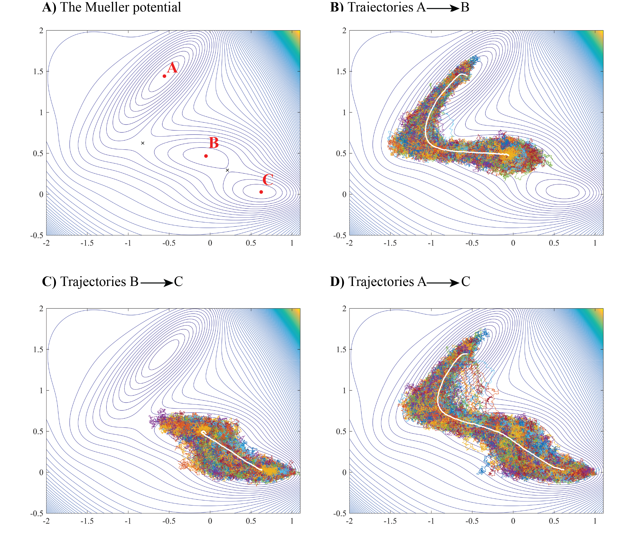
Figure 1: Langevin bridge trajectories on the Mueller potential. (A) Contour plot of the Mueller potential, with the three minima labeled A, B, and C, and the two saddle points between those minima indicated with an x. 500 converged trajectories between the minima A and B (B), B and C (C), and A and C (D). The unweighted mean trajectories are shown in white.

.

The Mueller potential is a standard benchmark potential to check the validity of methods for generating transition paths. It is a two dimensional potential given by

$$U(x,y)=\sum_{i=1}^{4}A_{i}\exp\left(a_{i}(x-x_{i}^{0})^{2}+b_{i}(x-x_{i}^{0})(y-y_{i}^{0})+c_{i}(y-y_{i}^{0})^{2}\right)$$ (25)

with

$$A=(-200,-100,-170,15)\ \ \ a=(-1,-1,-6.5,0.7)\ \ \ b=(0,0,11,0.6)$$ (26)

This potential has 3 local minima denoted by A,B,C, separated by two barriers (Fig.1). The effective potential $V(x,y)$ can be calculated analytically, as well as its gradient. Equations (18), (22) and (23) can easily be solved numerically. We display only the trajectories generated by (23). The simulation time $t_{f}$ is chosen so that we observe a small waiting time around the initial as well as the final point, namely $t_{f}=0.15$. We use 50 points for the integration over $u$. We display a sample of 500 trajectories obtained from eq. (23) with $t_{f}=0.15,\ dt=10^{-4},\ D=1$ at temperature $T=5$. We can compute the average trajectory as well as its variance. These trajectories are displayed on Fig. 1, where we plot the AB, BC and AC trajectories.

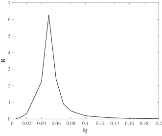
Figure 2: The quality factor $R$ plotted as a function of the total duration of the transition $t_{f}$, for the AB trajectories.

To assess the quality of the approximations, we check the criterion (24). For the trajectories AB, we obtain $R\approx 5.310^{-2}$, $R\approx 0.68$ for BC and $R\approx 1.13$ for AC. Therefore, the approximation is quite reliable for the AB trajectories, but less for the others. In fact, it is instructive to study the accuracy of the method when varying $t_{f}$. For that matter, in Fig. 2, we plot the factor $R$ as a function of $t_{f}$, for the AB transition. We see that for both small and large $t_{f}$, the factor $R$ is small, with a maximum at $t_{f}\approx 0.05$. For small $t_{f}$, the trajectories fluctuate around the straight line trajectory joining A to B through high barriers (see Fig. 1A). For large $t_{f}$, the trajectories fluctuate around the potential energy valley joining A to B. As $t_{f}$ increases from small values, the ensemble of trajectories include trajectories going through the high barrier and through the valley, and at $t_{f}\approx 0.05$, there is a strong mixing of both types of trajectories, giving rise to a large value of $R$. When $t_{f}$ increases further, the trajectories going through the barrier disappear from the ensemble, and only valley trajectories remain, yielding a decrease of $R$.

3.2 The Mexican hat potential

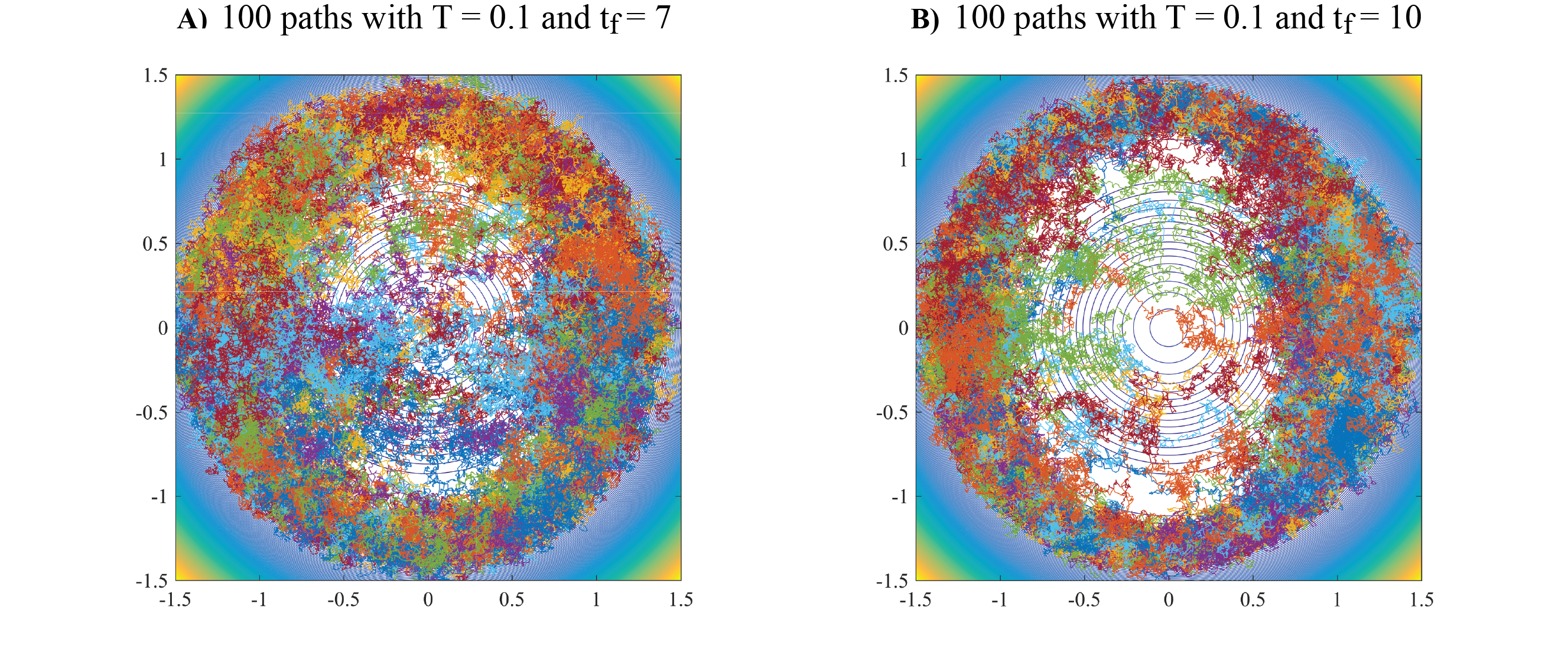
Figure 3: Langevin bridge trajectories on the Mexican hat potential. (A) 100 converged trajectories, all starting at $(-1,0)$ and ending at $(1,0)$, and generated at temperature $T=0.1$ with a duration $t_{f}=7$ . Note that with this short transition time, many trajectories go through the barrier region. (B) Same as in (A), but with $t_{f}$ now set to 10. Most of the trajectories now follow the circle of minima; those trajectories are nearly equally divided into two groups, those that follow the upper side of the circle (44), and those that follow the lower side (47) (see text for details).

.

The potential of the Mexican hat is given by

$$U(x,y)=\frac{1}{4}(x^{2}+y^{2}-1)^{2}$$ (27)

and has therefore a circle of minima for $x^{2}+y^{2}=1$ with $U=0$ and a maximum at $(0,0)$ with energy $U=1/4$. Again we solve equations (23), using 50 points for the $u$ integral. Given the small barrier of this potential $\Delta U=1/4$, we go to low temperature. On Fig.3A, we plot 100 trajectories, generated at temperature $T=0.1$, starting at $(-1,0)$ and all ending at $(1,0)$. The total time is $t_{f}=7$ and the time step is $dt=10^{-4}$. The quality criterion (24) gives $R=0.345$. The trajectories divide into three dominant groups, those that take a northern route (30), those that take a southern route (40) along the circle of minima, and those that go directly through the energy barrier (30). The distribution into those three groups was decided based on the mean value $Y_{mean}$ for the $y$ coordinates along the trajectories. If we take a longer duration, the fraction of trajectories that go through the central barrier decreases. For example, for $t_{f}=10$, there are only 9 of those trajectories , as seen on Fig. 3B. The quality criterion is then $R=0.266$.

4 Conclusions

In summary, we show here a novel method to generate ab initio transition path trajectories using a formalism called Conditioned Langevin dynamics. The most crucial parameter of the theory is the total length of the simulation, which must be carefully chosen so as to allow short waiting times around both the initial and final states. We define a quality criterion R that can be calculated a posteriori to see if the approximation made to solve the underlying PDE is justified or not. Here we have tested the method on simple one- or two-dimensional potentials, but our aim is to use it in more complicated situations, such as conformational transitions in proteins.

Proteins are small biopolymers (up to a few hundred amino-acids) that do not stay in one of their two states (e.g. native or denatured, open or closed, apo or holo in the allosteric picture), but rather make unfrequent stochastic transitions between them. They are usually represented in a coarse-grained manner using one or two beads per amino-acid. The picture which emerges is that of the system staying for a long time in one of the minima and then making stochastically rapid transitions to the other minimum. It follows that for most of the time, the system performs harmonic oscillations in one of the wells, which can be described by normal mode analysis. Rarely, there is a very short but interesting physical phenomenon, where the system makes a fast transition between minima. This picture has been confirmed by single molecule experiments, where the waiting time in one state can be measured, although the time for crossing is so short that it cannot be resolved ⁴⁷. This scenario has also been confirmed recently by very long millisecond molecular dynamics simulations which for the first time show spontaneous thermal folding-unfolding events ⁴⁸.

It is possible to model this behavior using a an energy function that is based on a simplified Elastic Network Model that is a mixture of two Elastic Networks centered around each of the two states of the macromolecule ^{8, 49}. We will present the results of the Conditioned Langevin Equation applied to this situation in a forthcoming paper.

5 Acknowledgements

MD acknowledges financial support from the Agence Nationale de la Recherche (ANR) through the program Bip-Bip.

References

- Eyring 1935 Eyring, H. The activated complex and the absolute rate of chemical reactions. Chem. Rev. 1935, 17, 65–77
- Wigner 1938 Wigner, E. The transition state method. Trans. Faraday Soc. 1938, 34, 29–41
- E and Vanden-Eijnden 2010 E, W.; Vanden-Eijnden, E. Transition-path theory and path-finding algorithms for the study of rare events. Annu Rev Phys Chem 2010, 61, 391–420
- E and Vanden-Eijnden 2006 E, W.; Vanden-Eijnden, E. Towards a theory of transition paths. J. Stat. Phys. 2006, 123, 503––23
- Vanden-Eijnden 2014 Vanden-Eijnden, E. Transition path theory. Adv. Exp. Med. Biol. 2014, 797, 91–100
- Kim et al. 2002 Kim, M.; Jernigan, R.; Chirikjian, G. Efficient generation of feasible pathways for protein conformational transitions. Biophys. J. 2002, 83, 1620–1630
- Weiss and Levitt 2009 Weiss, D. R.; Levitt, M. Can morphing methods predict intermediate structures? J. Mol. Biol. 2009, 385, 665–674
- Maragakis and Karplus 2005 Maragakis, P.; Karplus, M. Large amplitude conformational change in proteins explored with a plastic network model: adenylate kinase. J. Mol. Biol. 2005, 352, 807–822
- Zheng et al. 2007 Zheng, W.; Brooks, B.; Hummer, G. Protein conformational transitions explored by mixed elastic network models. Proteins: Struct. Func. Bioinfo. 2007, 69, 43–57
- Tekpinar and Zheng 2010 Tekpinar, M.; Zheng, W. Predicting order of conformational changes during protein conformational transitions using an interpolated elastic network model. Proteins: Struct. Func. Bioinfo. 2010, 78, 2469–2481
- Pinski and Stuart 2010 Pinski, F.; Stuart, A. Transition paths in molecules: gradient descent in pathspace. Journal of Chemical Physics 2010, 132, 184104
- Jonsson et al. 1998 Jonsson, H.; Mills, G.; Jacobsen, K. W. In Classical and Quantum Dynamics in Condensed Phase Simulations; Berne, B. J., Ciccotti, G., Coker, D. F., Eds.; World Scientific: Singapore, 1998; Chapter 16, pp 385–404
- Henkelman et al. 2000 Henkelman, G.; Uberuaga, B.; Jonsson, H. A climbing image nudged elastic band method for finding saddle points and minimum energy paths. J. Chem. Phys. 2000, 113, 9901–9904
- Sheppard et al. 2008 Sheppard, D.; Terrell, R.; Henkelman, G. Optimization methods for finding minimum energy paths. J. Chem. Phys. 2008, 128, 134106
- E et al. 2002 E, W.; Ren, W.; Vanden-Eijnden, E. String method for the study of rare events. Phys. Rev. B 2002, 66, 052301
- Ren et al. 2005 Ren, W.; Vanden-Eijnden, E.; Maragakis, P.; E, W. Transition pathways in complex systems: Application of the finite-temperature string method to the alanine dipeptide. J. Chem. Phys. 2005, 123, 134109
- E et al. 2007 E, W.; Ren, W.; Vanden-Eijnden, E. Simplified and improved string method for computing the minimum energy paths in barrier-crossing events. J. Chem. Phys. 2007, 126, 164103
- Vanden-Eijnden and Venturoli 2009 Vanden-Eijnden, E.; Venturoli, M. Revisiting the finite temperature string method for the calculation of reaction tubes and free energies. J. Chem. Phys. 2009, 130, 194103
- Ren and Vanden-Eijnden 2013 Ren, W.; Vanden-Eijnden, E. A climbing string method for saddle point search. J. Chem. Phys. 2013, 138, 134105
- Maragliano et al. 2014 Maragliano, L.; Roux, B.; Vanden-Eijnden, E. Comparison between Mean Forces and Swarms-of-Trajectories String Methods. J. Chem. Theory Comput. 2014, 10, 524–533
- Maragliano et al. 2006 Maragliano, L.; Fischer, A.; Vanden-Eijnden, E.; Ciccotti, G. String method in collective variables: minimum free energy paths and isocommittor surfaces. J. Chem. Phys. 2006, 125, 24106
- Pan et al. 2008 Pan, A.; Sezer, D.; Roux, B. Finding transition pathways using the string method with swarms of trajectories. J. Phys. Chem. B. 2008, 112, 3432–3440
- Matsunaga et al. 2012 Matsunaga, Y.; Fujisaki, H.; Terada, T.; Furuta, T.; Moritsugu, K.; Kidera, A. Minimum free energy path of ligand-induced transition in adenylate kinase. PLoS Comput. Biol. 2012, 8, e1002555
- Branduardi and Faraldo-Gomez 2013 Branduardi, D.; Faraldo-Gomez, J. D. String method for calculation of minimum free-energy paths in Cartesian space in freely-tumbling systems. J. Chem. Theory Comput. 2013, 9, 4140–4154
- Olender and Elber 1996 Olender, R.; Elber, R. Calculation of classical trajectories with a very large time step: formalism and numerical examples. J. Chem. Phys. 1996, 105, 9299––9315
- Eastman et al. 2001 Eastman, P.; Gronbech-Jensen, N.; Doniach, S. Simulation of protein folding by reaction path annealing. J. Chem. Phys. 2001, 114, 3823
- Franklin et al. 2007 Franklin, J.; Koehl, P.; Doniach, S.; Delarue, M. MinActionPath: maximum likelihood trajectory for large-scale structural transitions in a coarse grained locally harmonic energy landscape. Nucl. Acids. Res. 2007, 35, W477–W482
- Faccioli et al. 2006 Faccioli, P.; Sega, M.; Pederiva, F.; Orland, H. Dominant pathways in protein folding. Phys. Rev. Lett. 2006, 97, 108101
- Vanden-Eijnden and Heymann 2008 Vanden-Eijnden, E.; Heymann, M. The geometric minimum action method for computing minimum energy paths. J. Chem. Phys. 2008, 128, 061103
- Zhou et al. 2008 Zhou, X.; Ren, W.; E, W. Adaptive minimum action method for the study of rare events. J. Chem. Phys. 2008, 128, 104111
- Chandrasekaran et al. 2016 Chandrasekaran, S.; Dhas, J.; Dokholyan, N.; Carter Jr, C. A modified PATH algorithm rapidly generates transition states comparable to those found by other well established algorithms. Struct. Dyn. 2016, 3, 012101
- Pratt 1986 Pratt, L. A statistical method for identifying transition states in high dimensional problems. J. Chem. Phys. 1986, 85, 5045––48
- Bolhuis et al. 2002 Bolhuis, P.; Dellago, C.; Geissler, P. L.; Chandler, D. Transition path sampling: throwing ropes over rough mountain passes, in the dark. Annu. Rev. Phys. Chem. 2002, 53, 291–318
- Chodera et al. 2007 Chodera, J.; Singhal, N.; Pande, V.; Dill, K.; Swope, W. Automatic discovery of metastable states for the construction of Markov models of macromolecular conformational dynamics. J. Chem. Phys. 2007, 126, 155101
- Bowman et al. 2009 Bowman, G.; Beauchamp, K.; Boxer, G.; Pande, V. Progress and challenges in the automated construction of Markov state models for full protein systems. J. Chem. Phys. 2009, 124101
- Pande et al. 2010 Pande, V.; Beauchamp, K.; Bowman, G. Everything you wanted to know about Markov State Models but were afraid to ask. Methods 2010, 52, 99–105
- Orland 2011 Orland, H. Generating transition paths by Langevin bridges. J. Chem. Phys. 2011, 134, 174114
- Kampen 1992 Kampen, N. V. Stochastic Processes in Physics and Chemistry; North–Holland: Amsterdam, The Netherlands, 1992
- Zwanzig 2001 Zwanzig, R. Nonequilibrium Statistical Mechanics; Oxford University Press: Oxford, United Kingdom, 2001
- Doob 1957 Doob, J. Conditional Brownian motion and the boundary limits of harmonic functions. Bull. Soc. Math. France 1957, 85, 431–458
- Fitzsimmons et al. 1992 Fitzsimmons, P.; Pitman, J.; Yor, M. Seminar on Stochastic Processes, 1992; Birkhaeuser: Boston, MA, USA, 1992
- Majumdar and Orland 2015 Majumdar, S.; Orland, H. Effective Langevin equations for constrained stochastic processes. J. Stat. Mech. Theor. Exp. 2015, 2015, P06039
- Jensen 1906 Jensen, J. Sur les fonctions convexes et les inégalités entre les valeurs moyennes. Acta Math. 1906, 30, 175–193
- Gopich and Szabo 2006 Gopich, I.; Szabo, A. Theory of the statistics of kinetic transitions with application to single-molecule enzyme catalysis. J. Chem. Phys. 2006, 124, 154712
- Kim and Netz 2015 Kim, W.; Netz, R. The mean shape of transition and first-passage paths. J. Chem. Phys. 2015, 143, 224108
- 46 Carlon, E.; Orland, H. submitted
- Chung et al. 2012 Chung, H.; McHale, K.; Louis, J.; Eaton, W. Single–molecule fluorescence experiments determine protein folding transition path times. Science 2012, 335, 981–984
- Lindorff-Larsen et al. 2011 Lindorff-Larsen, K.; Piana, S.; Dror, R.; Shaw, D. How Fast-Folding Proteins Fold. Science 2011, 334, 517–520
- Das et al. 2014 Das, A.; Gur, M.; Cheng, M. H.; Jo, S.; Bahar, I.; Roux, B. Exploring the Conformational Transitions of Biomolecular Systems Using a Simple Two-State Anisotropic Network Model. PLoS Comput. Biol. 2014, 10, e1003521