On Limiting Behavior of Stationary Measures for Stochastic Evolution Systems with Small Noise Intensity

Abstract

The limiting behavior of stochastic evolution processes with small noise intensity $\epsilon$ is investigated in distribution-based approach. Let $\mu^{\epsilon}$ be stationary measure for stochastic process $X^{\epsilon}$ with small $\epsilon$ and $X^{0}$ be a semiflow on a Polish space. Assume that $\{\mu^{\epsilon}:0<\epsilon\leq\epsilon_{0}\}$ is tight. Then all their limits in weak sense are $X^{0}-$invariant and their supports are contained in Birkhoff center of $X^{0}$. Applications are made to various stochastic evolution systems, including stochastic ordinary differential equations, stochastic partial differential equations, stochastic functional differential equations driven by Brownian motion or Lévy process.

T1This work was supported by the National Natural Science Foundation of China (NSFC)(Nos. 11371252, 11271356, 11371041, 11431014, 11401557), Research and Innovation Project of Shanghai Education Committee (No. 14zz120), Key Laboratory of Random Complex Structures and Data Science, Academy of Mathematics and Systems Science, CAS, and the Fundamental Research Funds for the Central Universities (No. WK0010000048).

, , and

t1Corresponding author

1 Introduction

Mumford [42] addressed that

“Stochastic differential equations are more fundamental and relevant to modeling the world than deterministic equations $\cdots$. A major step in making the equation more relevant is to add a small stochastic term. Even if the size of the stochastic term goes to 0, its asymptotic effects need not. It seems fair to say that all differential equations are better models of the world when a stochastic term is added and that their classical analysis is useful only if it is stable in an appropriate sense to such perturbations”. This shows that it is important to check the asymptotic stability of stochastic systems with small noise. For this purpose, a basic method is to study the stationary measures and their limit measures. The latters are called zero-noise limits by Young [49] and Cowieson and Young [11], where they proved SRB measures can be realized as zero-noise limits. Huang, Ji, Liu and Yi [27, 28] have investigated stochastic ordinary differential equations with small white noise where the drift vector field is dissipative. They have shown that limiting measures are invariant for the flow generated by the drift vector field and their supports are in its global attractor. For non-degenerate noise, Freidlin and Wentzell [18] estimated the concentration of limiting measure for stationary measures via the large-deviation technique and proved that the stationary measure value $\mu^{\epsilon}(P)$ tends to zero for any subset $P$ not intersecting with any attractor for the drift vector field, which implies that any limiting measure will support on the global attractor of the drift vector field; Li and Yi [35, 36] have presented more precise estimation for stationary measures near the global attractor or outside of the global attractor via the Fokker-Planck equation and the level set method developed in [28], which are applied by them to study systematic measures of biological network including degeneracy, complexity, and robustness. Hwang [31] proved limiting probability measure of Gibbs measures for gradient system with additive noise concentrates on the minimal energy states. Huang, Ji, Liu and Yi [30] have explored the stochastic stability of invariant sets and measures for gradient systems with noises.

This paper is intended to establish the close connection between deterministic dynamical systems and their stochastic perturbations by considering the limiting behavior of stationary measures for stochastic evolution systems with small random perturbations. These stochastic evolution systems $X^{\epsilon}(t,x)$ may be solutions of various stochastic differential equations driven by white or Lévy noise with the intensity $\epsilon$. The corresponding solution of deterministic equations is denoted by $X^{0}(t,x)$. Let $\mu^{\epsilon}$ be the stationary probability measure of $X^{\epsilon}(t,x)$. We prove that all their limits of stationary measures $\mu^{\epsilon}$ of $X^{\epsilon}$ are $X^{0}-$invariant and their supports are contained in the Birkhoff center of $X^{0}$ as $\epsilon$ tends to zero (see Theorem 2.1). For various stochastic differential equations with small noise intensity, we prove the probability convergence property and provide the existence of stationary measures and their tightness and applications to all corresponding stochastic systems (see sections 3-5). Usually, a global attractor for finite dimensional system has positive Lebesgue measure if it is not a globally stable equilibrium, however, the Birkhoff center always has zero Lebesgue measure for dissipative system. Compared to the existing results, which mostly focus on SODEs with non-degenerate noise, ours gives much more precise positions for limiting measures to support. We note that our result is the best if we don’t put any restriction to types of noise because we can construct a diffusion term such that a sequence of stationary measures weakly converges to a given invariant measure of the drift vector field (see Proposition 3.2 and Remark 9). As far as we know, among all existing examples (see, for example, [18, 27, 31]), the limiting measures support at stable orbits, such as, stable equilibrium or closed orbits. A natural question arises : when a dissipative drift vector field has no stable motion in its global attractor, where does any limiting measure support? Utilizing our result, we construct Bernoulli’s lemniscate with non-degenerate noise such that stationary measures weakly converge to a delta measure at a saddle of the drift vector field, however, the global attractor in this case is the closed domain surrounded by the lemniscate of Bernoulli (see Example 3). In May-Leonard system perturbed by a one dimensional white noise (see Example 4), we have proved that the limiting measures will support at the three saddles when the deterministic May-Leonard system admits a heteroclinic cycle. Also, from this example, the limiting measures can be distinguished by different initial values because of the various kinds of asymptotic behavior for deterministic equations. In a word, limiting measures always support at “most relatively stable positions”.

This article is organized as follows. In section 2, we present the framework to study the limiting measures of stationary measures for stochastic evolution processes and their supports. From sections 3–5, we prove the probability convergence, the existence of stationary measures and their tightness for various stochastic differential equations. Specially, in section 3, we deal with all these problems of stochastic ordinary differential equations (SODEs). In section 4, we investigate stochastic reaction-diffusion equations, stochastic $2D$ Navier-Stokes equations and stochastic Burgers type equations driven by Brownian motions or Lévy process. In sections 5, we consider a class of stochastic functional differential equations (SFDEs). Section 6 collects the basic properties on invariant measures of deterministic flow.

Here and throughout of this article, we will use the same symbol $|\cdot|$ to denote Euclidean norm of a vector or the operator norm of a matrix. Sometimes we will write $X^{\epsilon}(t,x)$, $X^{0}(t,x)$ as $X^{\epsilon}_{t}(x)$, $X^{0}_{t}(x)$, respectively, unless noted otherwise.

2 General framework to study limiting measures

In this section, we will give general criterion on studying limiting measures of stationary measures for stochastic evolution processes and describe their concentration.

Let $(\Omega,\mathcal{F},\mathbb{P})$ be a probability space, $(M,\rho)$ be a Polish space and $\mathcal{B}(M)$ be the Borel $\sigma-$algebra on $M$. Assume that $\Phi_{t}(x):=X^{0}_{t}(x)$ is a deterministic semi-dynamical system (semiflow) on $(M,\rho)$ and for $0<\epsilon\ll 1$, $X^{\epsilon}_{t}(x)$ is a noise driven process on $(M,\rho)$ with noise intensity $\epsilon$.

Throughout this article we assume that $\Phi:\mathbb{R}_{+}\times M\longrightarrow M$ is a mapping with the following properties

(i) $\Phi_{\cdot}(x)$ is continuous, for all $x\in M$,

(ii) $\Phi_{t}(\cdot)$ is Borel measurable, for all $t\in\mathbb{R}_{+}$,

(iii) $\Phi_{0}={\rm id}$, $\Phi_{t}\circ\Phi_{s}(x)=\Phi_{t+s}(x)$, for all $t,s\in\mathbb{R}_{+}$, $x\in M$. Here $\circ$ denotes composition of mappings.

Let $\{X^{\epsilon}_{t}(x),t\geq 0\}$ be a family of processes with initial value $x$ on state space $M$, $\epsilon\in(0,1]$. The probability transition function is defined as

$$P^{\epsilon}_{t}(x,A):=\mathbb{P}(X^{\epsilon}_{t}(x)\in A),t\geq 0,x\in M,A\in\mathcal{B}(M).$$

A probability measure $\mu^{\epsilon}$ on $\mathcal{B}(M)$ is called stationary (or invariant) with respect to $\{P^{\epsilon}_{t}\}_{t\geq 0}$ if

$$P^{\epsilon}_{t}\mu^{\epsilon}=\mu^{\epsilon}\ \textrm{for\ any}\>\>t\geq 0.$$

Let $\mathscr{I}^{\epsilon}$ denote the set of all stationary measures of the process $\{X^{\epsilon}_{t}\}_{t\geq 0}.$

For our purpose, a necessary condition is $X^{\epsilon}_{T}(x)\xlongrightarrow{\mathbb{P}}X^{0}_{T}(x)$ as $\epsilon\rightarrow 0$. For a technical reason, we impose the following Hypothesis.

Hypothesis (Probability Convergence): For any given compact set $K\subset M$, $T>0$ and $\delta>0$,

$$\lim_{\epsilon\to 0}\sup_{x\in K}\mathbb{P}\{\displaystyle\rho\big{(}X^{\epsilon}(T,x),\Phi(T,x)\big{)}\geq\delta\}=0.$$ (2.1)

Theorem 2.1.

Assume hypothesis (2.1) holds. If $\mu^{\epsilon_{i}}\in\mathscr{I}^{\epsilon_{i}}$, and $\mu^{\epsilon_{i}}\overset{w}{\rightarrow}\mu$ as $\epsilon_{i}\rightarrow 0$, then $\mu$ is an invariant measure of $\Phi$, i.e. $\mu\circ\Phi_{t}^{-1}=\mu$ for every $t\geq 0$. Moreover, this invariant probability measure $\mu$ is concentrated on $B(\Phi)$, where $B(\Phi):=\overline{\{x\in M:x\in\omega(x)\}}$ denotes the Birkhoff center of $\Phi$ (see the definition in Appendix).

Proof.

Let $\mu^{\epsilon_{i}}\overset{w}{\rightarrow}\mu$ as $\epsilon_{i}\rightarrow 0$. It suffices to prove that for any nonzero $g\in C_{b}(M)$ and $T>0$,

$$\int g(x)\mu\circ\Phi_{T}^{-1}(dx)=\int g(x)\mu(dx),$$

or equivalently,

$$\int g\big{(}\Phi(T,x)\big{)}\mu(dx)=\int g(x)\mu(dx).$$

Since $\{\mu^{\epsilon_{i}}\}$ is relatively compact, it is tight. For every $\eta>0$, there exists a compact set $K\subset M$ such that $\displaystyle\inf_{\epsilon_{i}}\mu^{\epsilon_{i}}(K)\geq 1-\frac{\eta}{\|g\|}$.

$$|\int g(x)\mu^{\epsilon_{i}}\circ\Phi(T,\cdot)^{-1}(dx)-\int g(x)\mu^{\epsilon_{i}}(dx)|$$

$$= |\int\mathbb{E}g\big{(}\Phi(T,x)\big{)}\mu^{\epsilon_{i}}(dx)-\int\mathbb{E}g\big{(}X^{\epsilon_{i}}(T,x)\big{)}\mu^{\epsilon_{i}}(dx)|$$

$$\leq \int\mathbb{E}|g\big{(}\Phi(T,x)\big{)}-g\big{(}X^{\epsilon_{i}}(T,x)\big{)}|\mu^{\epsilon_{i}}(dx)$$

$$\leq \int\mathbb{E}|I_{K}(x)[g(\Phi(T,x))-g(X^{\epsilon_{i}}(T,x))]|\mu^{\epsilon_{i}}(dx)+2\eta.$$

$\widetilde{K}:=\Phi(T\times K)\subset M$ is a compact set since $\Phi(T,x)$ is continuous on $x$. We claim that there exists $\delta>0$ such that $\forall y,z\in M$ with $z\in\widetilde{K}$ and $\rho(y,z)<\delta$, one has

$$|g(y)-g(z)|<\eta.$$

If not, then there exist $\eta_{0}>0$ and $y_{n}\in M$ and $z_{n}\in\widetilde{K}$ with $\rho(y_{n},z_{n})<\frac{1}{n}$ such that $|g(y_{n})-g(z_{n})|\geq\eta_{0}$, $n=1,2,\cdots$. The compactness of $\widetilde{K}$ and $\{z_{n}\}\subset\widetilde{K}$ imply that, without loss of generality, $z_{n}\rightarrow z_{0}\in\widetilde{K}$ as $n\rightarrow\infty$. Therefore, it follows from $\rho(y_{n},z_{n})<\frac{1}{n}$ that $y_{n}\rightarrow z_{0}$. By the continuity of $g$, letting $n\rightarrow\infty$, we have

$$0=|g(z_{0})-g(z_{0})|\geq\eta_{0},$$

a contradiction.

Hence one can derive that

$$\int\mathbb{E}|I_{K}(x)[g\big{(}\Phi(T,x)\big{)}-g\big{(}X^{\epsilon_{i}}(T,x)\big{)}]|\mu^{\epsilon_{i}}(dx)$$

$$= \int_{K}\mathbb{E}|I_{\{\rho(\Phi(T,x),X^{\epsilon_{i}}(T,x))\geq\delta\}}(\omega)[g\big{(}\Phi(T,x)\big{)}-g\big{(}X^{\epsilon_{i}}(T,x)\big{)}]|\mu^{\epsilon_{i}}(dx)$$

$$+\int_{K}\mathbb{E}|I_{\{\rho(\Phi(T,x),X^{\epsilon_{i}}(T,x))<\delta\}}(\omega)[g\big{(}\Phi(T,x)\big{)}-g\big{(}X^{\epsilon_{i}}(T,x)\big{)}]|\mu^{\epsilon_{i}}(dx)$$

$$\leq 2\|g\|\displaystyle\sup_{x\in K}\mathbb{P}\Big{(}\displaystyle\ \rho\big{(}X^{\epsilon_{i}}(T,x),\Phi(T,x)\big{)}\geq\delta\Big{)}+\eta.$$

Therefore, by the hypothesis (2.1), one can show that

$$\displaystyle\limsup_{\epsilon_{i}\rightarrow 0}|\int g(x)\mu^{\epsilon_{i}}\circ\Phi(T,\cdot)^{-1}(dx)-\int g(x)\mu^{\epsilon_{i}}(dx)|$$

$$\leq 2\|g\|\displaystyle\lim_{\epsilon_{i}\rightarrow 0}\displaystyle\sup_{x\in K}\mathbb{P}\big{\{}\displaystyle\ \rho\big{(}X^{\epsilon_{i}}(T,x),\Phi(T,x)\big{)}\geq\delta\big{\}}+\eta+2\eta=3\eta.$$

Since $\eta>0$ is arbitrary and $\mu^{\epsilon_{i}}\xlongrightarrow{w}\mu$, hence $\int g(x)\mu\circ\Phi(T,\cdot)^{-1}(dx)=\int g(x)\mu(dx)$. This shows that $\mu$ is an invariant probability measure of the semiflow $\Phi$.

It remains to prove that $\mu(B(\Phi))=1$. Indeed, the result of this fact relies on the following well-known lemma, the Poincaré recurrence theorem.   ∎

Lemma 2.1.

The support of semiflow $\Phi$-invariant probability measure $\mu$ is contained in $B(\Phi)$. Consequently this implies that $\mu(B(\Phi))=1$.

The above result is a slightly variant version of the Poincaré recurrence theorem (see e.g., Mañé [38, Theorem 2.3, p.29]) to obtain the concentration of invariant measures. For readers’ convenience, we also give a self-contained proof of Lemma 2.1 which is postponed to Appendix.

Remark 1.

Observing the proof of Theorem 2.1, we only need to prove the probability convergence property for a compact set $K$ satisfying the definition of tightness. This remark will be used in SPDEs of section 4.

In order to apply Theorem 2.1 to various stochastic differential equations, the probability convergence (2.1) and the existence of stationary measures for $X^{\epsilon}_{t}(x)$ and their tightness are needed to be proved. In the rest of this paper, we will check them for various stochastic evolution systems.

3 ODEs driven by Lévy noise

Let $(\Omega,\mathcal{F},\mathbb{P})$ be a probability space equipped with a filtration $\{\mathcal{F}_{t},t\geq 0\}$ satisfying the usual conditions, $W=\{W_{t},t\geq 0\}$ a $k$-dimensional Wiener process and $N$ a Poisson random measure on $\mathbb{R}_{+}\times(\mathbb{R}^{l}\backslash\{O\})$ with the $\sigma$-finite intensity measure $\nu$ on $\mathbb{R}^{l}\backslash\{O\}$, and denote its associated compensator as $\tilde{N}(dt,dy)=N(dt,dy)-\nu(dy)dt$. Denote by $(L_{2}(\mathbb{R}^{k},\mathbb{R}^{m}),\|\cdot\|_{2})$ the Hilbert space of all Hilbert-Schmidt operators from $\mathbb{R}^{k}$ to $\mathbb{R}^{m}$. Actually, $L_{2}(\mathbb{R}^{k},\mathbb{R}^{m})$ is $m\times k$ matrices set.

Consider the following SODEs driven by a Lévy process

$$\begin{split}dX^{\epsilon,x}(t)=&b(X^{\epsilon,x}(t))dt+\epsilon\sigma(X^{\epsilon,x}(t))dW_{t}\\ &+\epsilon\int_{|y|_{\mathbb{R}^{l}}<c}F(X^{\epsilon,x}(t-),y)\tilde{N}(dt,dy)\end{split}$$ (3.1)

with initial condition $X^{\epsilon,x}(0)=x\in\mathbb{R}^{m}$ and $\epsilon,c>0$. The mappings $b:\mathbb{R}^{m}\rightarrow\mathbb{R}^{m}$ and $\sigma:\mathbb{R}^{m}\rightarrow L_{2}(\mathbb{R}^{k},\mathbb{R}^{m})$ are $\mathcal{B}(\mathbb{R}^{m})$ measurable functions, $F:\mathbb{R}^{m}\times\mathbb{R}^{l}\rightarrow\mathbb{R}^{m}$ is $\mathcal{B}(\mathbb{R}^{m})\otimes\mathcal{B}(\mathbb{R}^{l})$ measurable function.

$b$, $\sigma$ and $F$ are called to satisfy local Lipschitz condition, respectively, if for every integer $n\geq 1$, there is a positive constant $L_{1}(n)$ such that for all $x,y\in\mathbb{R}^{m}$ with $|x|\leq n$ and $|y|\leq n$,

$$|b(x)-b(y)|^{2}\leq L_{1}(n)|x-y|^{2},$$ (3.2)

$$\|\sigma(x)-\sigma(y)\|_{2}^{2}\leq L_{1}(n)|x-y|^{2},$$ (3.3)

$$\int_{{}_{\|z\|_{\mathbb{R}^{l}}<c}}|F(x,z)-F(y,z)|^{2}\nu(dz)\leq L_{1}(n)|x-y|^{2},$$ (3.4)

respectively. In addition, we say that $F$ satisfies local growth condition, if for every integer $n\geq 1$, there is a positive constant $L_{2}(n)$ such that for all $|x|\leq n$,

$$\int_{{}_{\|z\|_{\mathbb{R}^{l}}<c}}|F(x,z)|^{2}\nu(dz)\leq L_{2}(n)(1+|x|^{2}).$$ (3.5)

If $L_{i}(n)$, $i=1,2$ are independent of $n$, we say that the coefficient functions admit global Lipschitz and linear growth conditions.

For a $C^{2}$ scalar function $V$, and $\epsilon\geq 0$, we define

$$\mathcal{L}^{\epsilon}V(x):= \langle\nabla V(x),b(x)\rangle+\frac{\epsilon^{2}}{2}\displaystyle\sum_{i,j=1}^{m}a_{ij}(x)\frac{\partial^{2}V(x)}{\partial x_{i}\partial x_{j}}$$

$$+\int_{|y|_{\mathbb{R}^{l}}<c}\big{(}V(x+\epsilon F(x,y))-V(x)-\langle\nabla V(x),\epsilon F(x,y)\rangle\big{)}\nu(dy),$$

where $A(x)=(a_{ij}(x)):=\sigma(x)\sigma^{T}(x)$ is the diffusion matrix. Let $\mathcal{S}^{\epsilon}$ denote the set of all stationary measures of (3.1) for a given $\epsilon$. The following is the main result of this section.

Theorem 3.1 (Support on Limiting Measures).

Let $b(x)$, $\sigma(x)$ and $F(x,y)$ in (3.1) be locally Lipschitz continuous and locally linear growth, and $F(x,y)$ locally bounded with respect to $(x,y)$. Suppose that there exists a nonnegative function $V(x)\in C^{2}(\mathbb{R}^{m})$ such that

$$\inf_{|x|>R}V(x)\rightarrow+\infty,\quad\textrm{as}\ R\rightarrow\infty,\ {\rm and}$$ (3.6)

$$\sup_{|x|>R}\mathcal{L}^{\epsilon}V(x)\leq-A_{R}\rightarrow-\infty\>\textrm{as}\>R\rightarrow\infty.$$ (3.7)

If $\mu^{\epsilon_{i}}_{x_{i}}\in\mathcal{S}^{\epsilon_{i}},$ and $\mu^{\epsilon_{i}}_{x_{i}}\overset{w}{\rightarrow}\mu$ as $\epsilon_{i}\rightarrow 0$, then $\mu$ is an invariant measure of $X^{0}(t)$, which supports on the Birkhoff center $B(X^{0})$.

The proof of the Theorem 3.1 follows from subsections 3.1 and 3.2.

3.1 The criterion for probability convergence

By standard arguments, we have

Lemma 3.1.

Suppose that the coefficient functions $b,\sigma$ and $F$ admit global Lipschitz and linear growth conditions with positive constant $L$. Then the system (3.1) admits a unique strong solution $X^{\epsilon,x}=\{X^{\epsilon,x}(t):t\geq 0\}$, which is adapted and has càdlàg sample paths. Moreover, for every fixed $T>0$, there is a constant $D_{L,T}$ such that for each $x\in\mathbb{R}^{m}$,

$$\sup_{\epsilon\in(0,1]}\ \sup_{t\in[0,T]}\mathbb{E}|X^{\epsilon,x}(t)|^{2}\leq D_{L,T}(1+|x|^{2}).$$ (3.8)

Denote by $X^{0,x}(t)$ the solution for (3.1) as $\epsilon=0$. Then we have

Proposition 3.1.

Suppose that the coefficient functions $b,\sigma$ and $F$ admit global Lipschitz and linear growth conditions with positive constant $L$. Then there exists a constant $D^{*}_{L,T}$ such that for every $\epsilon\in(0,1]$

$$\mathbb{E}[\displaystyle\sup_{0\leq t\leq T}|X^{\epsilon,x}(t)-X^{0,x}(t)|^{2}]\leq D^{*}_{L,T}\epsilon^{2}(1+|x|^{2})$$

for all $x\in\mathbb{R}^{m}$.

Theorem 3.2.

Let $b$, $\sigma$ and $F$ be locally Lipschitz continuous and locally linear growth. If there exist a function $V\in C^{2}(\mathbb{R}^{m},\mathbb{R}_{+})$, $\epsilon_{0}>0$ and a constant $c^{*}<+\infty$, such that (3.6) and

$$\mathcal{L}^{\epsilon}V(x)\leq c^{*}V(x),\quad\forall\epsilon\in[0,\epsilon_{0}]$$ (3.9)

hold. Then there exists a global unique solution $X^{\epsilon,x}(t)$ to (3.1) for all $x\in\mathbb{R}^{m}$ and all $\epsilon\in[0,\epsilon_{0}]$. Moreover the hypothesis (2.1) holds, that is, for any given compact set $K\subset\mathbb{R}^{m}$, $T>0$ and $\delta>0$,

$$\lim_{\epsilon\to 0}\sup_{x\in K}\mathbb{P}\{|X^{\epsilon,x}(T)-X^{0,x}(T)|\geq\delta\}=0.$$

Proof.

For the global existence and uniqueness of solution to (3.1) we refer to a similar proof in Khasminskii [34, Theorem 1.1.3 and Theorem 3.3.5], for instance. Without loss of generality, we assume $c^{*}>0$. Let $\tau_{n}^{\epsilon,x}=\inf\{t:|X^{\epsilon,x}(t)|>n\}$ and $\tau_{n}^{0,x}=\inf\{t:|X^{0,x}(t)|>n\}$. It is easy to see that $\tau_{n}^{\epsilon,x}$ and $\tau_{n}^{0,x}$ nondecreasingly tend to infinity as $n\rightarrow\infty$.

For each $n\in\mathbb{N}^{*}$, let $S^{n}(r)$ be a nonincreasing $C^{\infty}$ function with values in $[0,1]$ such that

$$S^{n}(r)=\begin{cases}1&\textrm{if}\ r\in[0,n],\\ \frac{n+\frac{1}{2}}{r}&\textrm{if}\ r\in[n+1,+\infty).\end{cases}$$

Construct functions

$$b_{n}(x)=b\big{(}xS^{n}(|x|)\big{)},$$ (3.10)

$\sigma_{n}(x)$ and $F_{n}(x,y)$ similarly. Then $b_{n}(x)$, $\sigma_{n}(x)$ and $F_{n}(x,y)$ clearly satisfy global Lipschitz and linear growth conditions. Let $X_{n}^{\epsilon,x}(t)$ be the solution associated with functions $b_{n}(x)$, $\sigma_{n}(x)$ and $F_{n}(x,y)$. It is easy to see that $X^{\epsilon,x}(t)=X_{n}^{\epsilon,x}(t)$ for $t\leq\tau_{n}^{\epsilon,x}$. Repeating the proof in Khasminskii [34, Theorem 3.5, p.76], we know that

$$\mathbb{P}(\tau_{n}^{\epsilon,x}\leq T)\leq\frac{\exp(c^{*}T)V(x)}{\inf_{|y|>n}V(y)},$$

which implies that $\mathbb{P}(\tau_{n}^{\epsilon,x}\leq T)\rightarrow 0$ as $n\rightarrow\infty$ uniformly for $x\in K$. This shows that $\forall\eta>0$, $\exists N_{0}\in\mathbb{N}^{*}$, such that $\forall n\geq N_{0}$, we have $\displaystyle\sup_{x\in K}\mathbb{P}(\tau_{n}^{\epsilon,x}\leq T)<\eta$. The compactness of $K$ and continuity for solution $X^{0,x}(t)$ with respect to initial point ensure that there exists $N_{1}\in\mathbb{N}^{*}$, such that for all $n\geq N_{1}$,

$$\inf_{x\in K}\tau_{n}^{0,x}>T.$$

Now choosing $n\geq N_{0}\vee N_{1}$, we have

$$\displaystyle\sup_{x\in K}\mathbb{P}\{|X^{\epsilon,x}(T)-X^{0,x}(T)|\geq\delta\}$$

$$\leq \displaystyle\sup_{x\in K}\mathbb{P}\{|X^{\epsilon,x}(T)-X^{0,x}(T)|\geq\delta,T<\tau_{n}^{\epsilon,x}\wedge\tau_{n}^{0,x}\}$$

$$+\displaystyle\sup_{x\in K}\mathbb{P}(\tau_{n}^{\epsilon,x}\wedge\tau_{n}^{0,x}\leq T)$$

$$= \displaystyle\sup_{x\in K}\mathbb{P}\{|X_{n}^{\epsilon,x}(T)-X_{n}^{0,x}(T)|\geq\delta,T<\tau_{n}^{\epsilon,x}\wedge\tau_{n}^{0,x}\}$$

$$+\displaystyle\sup_{x\in K}\mathbb{P}(\tau_{n}^{\epsilon,x}\leq T)$$

$$\leq \frac{1}{\delta^{2}}\displaystyle\sup_{x\in K}\mathbb{E}|X_{n}^{\epsilon,x}(T)-X_{n}^{0,x}(T)|^{2}+\eta$$

$$\leq \displaystyle\sup_{x\in K}\frac{D^{*}_{L_{n},T}(1+|x|^{2})}{\delta^{2}}\epsilon^{2}+\eta$$

$$\leq 2\eta,\quad\forall\epsilon\in(0,\epsilon_{0}]$$

for some constant $\epsilon_{0}>0$. The proof is complete. ∎

3.2 The criteria on the existence of stationary measures and their tightness

Following the arguments as Khasminskii in [33, 34], we obtain the criterion on the tightness of a family of stationary measures for (3.1).

Theorem 3.3 (Tightness Criterion).

Suppose that $b(x)$, $\sigma(x)$ and $F(x,y)$ in (3.1) are locally Lipschitz continuous and locally linear growth, and $F(x,y)$ is locally bounded with respect to $(x,y)$, and that there exists a scalar function $V(x)\in C^{2}(\mathbb{R}^{m},\mathbb{R}_{+})$ such that (3.6) and (3.7) hold. Then for any $x\in\mathbb{R}^{m}$, there exists at least a stationary measure $\mu^{\epsilon}_{x}$ for every $\epsilon$, and the set $\mathcal{S}:=\bigcup\{\mathcal{S}^{\epsilon}:0<\epsilon\leq\epsilon_{0}\}$ of stationary measures is tight.

Proof.

For any fixed $x\in\mathbb{R}^{m}$, it follows from Theorem 3.2 that the solution $X^{\epsilon}(t,x)$ is globally defined on $[0,+\infty)$. For any $n\in\mathbb{N}^{*}$, we define stopping time $\tau_{n}^{\epsilon}=\inf\{t:|X^{\epsilon}(t,x)|>n\}$. Then Itô’s formula and Doob’s optional sampling theorem (see [1, 32]) imply that

$$\mathbb{E}V(X^{\epsilon}(t\wedge\tau_{n}^{\epsilon},x))-V(x)=\mathbb{E}\int_{0}^{t\wedge\tau_{n}^{\epsilon}}\mathcal{L}^{\epsilon}V(X^{\epsilon}(s,x))ds.$$

Since $V(x)\in C^{2}(\mathbb{R}^{m})$ and $F(x,y)$ is locally bounded, applying Taylor expansion and (3.5), we obtain

$$\sup_{\epsilon\in[0,\epsilon_{0}]}\int_{|y|_{\mathbb{R}^{l}}<c}\big{(}V(x+\epsilon F(x,y))-V(x)-\langle\nabla V(x),\epsilon F(x,y)\rangle\big{)}\nu(dy)<\infty.$$

By $V(x)\in C^{2}(\mathbb{R}^{m})$ again and (3.7), $C:=\displaystyle\sup_{\epsilon\in[0,\epsilon_{0}]}\sup_{x\in\mathbb{R}^{m}}\mathcal{L}^{\epsilon}V(x)<\infty$. Hence we have

$$\mathcal{L}^{\epsilon}V(X^{\epsilon}(s,x))\leq-I_{\{|X^{\epsilon}(s,x)|>R\}}A_{R}+C,$$

it is easy to get

$$A_{R}\mathbb{E}\int_{0}^{t\wedge\tau_{n}^{\epsilon}}I_{\{|X^{\epsilon}(s,x)|>R\}}ds\leq V(x)+Ct,$$

where we have used the condition (3.7). Since $t\wedge\tau_{n}^{\epsilon}\rightarrow t$ a.s. as $n\rightarrow\infty$, letting $n\rightarrow\infty$ and then changing the order of integration in the last inequality, we have for $t>0$,

$$\frac{1}{t}\int_{0}^{t}P^{\epsilon}(s,x,U_{R}^{c})ds\leq\frac{1}{A_{R}}\big{(}\frac{V(x)}{t}+C\big{)},$$ (3.11)

where $U_{R}^{c}=\{x\in\mathbb{R}^{m}:|x|>R\}$. This implies that

$$\lim_{R\rightarrow\infty}\liminf_{t\rightarrow\infty}\frac{1}{t}\int_{0}^{t}P^{\epsilon}(s,x,U_{R}^{c})ds=0.$$

Applying Khasminskii [34, Theorem 3.1, p.66], there exists at least a stationary measure $\mu_{x}^{\epsilon}$, which is produced by Krylov-Bogoliubov procedure, that is, $\mu_{x}^{\epsilon}$ is a weak limit of a subsequence of probability measures on $\mathbb{R}^{m}$ defined by

$$P^{\epsilon,t}(x,B)=\frac{1}{t}\int_{0}^{t}P^{\epsilon}(s,x,B)ds.$$

Denote by $\mathcal{S}^{\epsilon}_{x}$ the set of all their weak limits of probability measures $\{P^{\epsilon,t}(x,\cdot):t>0,\}$ and $\mathcal{S}^{\epsilon}:=\bigcup\{\mathcal{S}^{\epsilon}_{x}:x\in\mathbb{R}^{m}\}$ for $\epsilon\in(0,\epsilon_{0}]$. Pick any $\mu_{x}^{\epsilon}\in\mathcal{S}$. Then there are $\epsilon\in(0,\epsilon_{0}]$, $x\in\mathbb{R}^{m}$ and $t_{n}\rightarrow\infty$ such that $P^{\epsilon,t_{n}}(x,\cdot)\overset{w}{\rightarrow}\mu_{x}^{\epsilon}(\cdot)$ as $n\rightarrow\infty$, by the Portmanteau Theorem and (3.11), we obtain

$$\mu^{\epsilon}_{x}(U_{R}^{c})\leq\displaystyle\liminf_{n\rightarrow\infty}P^{\epsilon,t_{n}}(x,U_{R}^{c})\leq\frac{C}{A_{R}}.$$

Since $\lim_{R\rightarrow\infty}\frac{C}{A_{R}}=0$ uniformly in $\epsilon\in(0,\epsilon_{0}]$ by assumptions, the set $\mathcal{S}$ of stationary measures is tight. This completes the proof. ∎

Remark 2.

From our proof, the conclusions still hold if $C\leq 0$ and there is a constant $\gamma>0$ such that $A_{R}\geq\gamma>0$ for $R$ sufficiently large.

Remark 3.

Huang, Ji, Li and Yi [28] gave the estimate of stationary measures in the essential domain of a Lyapunov-like function in case $F\equiv 0$, which provides the criterion for the tightness of stationary measures.

Our results allow the nonlinear terms in (3.1) to be polynomial growth, which is stated as the following corollary.

Corollary 3.1.

Suppose that $b(x)$, $\sigma(x)$ and $F(x,y)$ in (3.1) are locally Lipschitz continuous and locally linear growth, and that $F(x,y)$ is locally bounded with respect to $(x,y)$. If there are positive constants $c_{1},c_{2}$ and $q\geq 2$ such that for $|x|$ sufficiently large, one has

$$\langle b(x),x\rangle\leq-c_{1}|x|^{q},$$

$$\frac{1}{2}\|\sigma(x)\|^{2}_{2}+\int_{|y|_{\mathbb{R}^{l}}<c}|F(x,y))|^{2}\nu(dy)\leq c_{2}|x|^{q},$$

then the conclusions of Theorems 3.2 and 3.3 hold.

Proof.

Define $V:\mathbb{R}^{m}\rightarrow\mathbb{R}_{+}$ by

$$V(x):=\frac{1}{2}\sum_{i=1}^{m}{(x^{i})}^{2}.$$

Then

$$\mathcal{L}^{\epsilon}V(x)= \langle b(x),x\rangle+\frac{\epsilon^{2}}{2}\|\sigma(x)\|^{2}_{2}+\epsilon^{2}\int_{|y|_{\mathbb{R}^{l}}<c}|F(x,y))|^{2}\nu(dy)$$

$$\leq-(c_{1}-\epsilon^{2}c_{2})|x|^{q}$$

$$\leq-\frac{c_{1}}{2}|x|^{q}$$

for $|x|$ sufficiently large and $\epsilon$ sufficiently small. It is easy to see that (3.6) and (3.7) and all other conditions in Theorems 3.2 and 3.3 hold. The proof is complete. ∎

It is easy to see that Theorem 3.1 follows immediately from Theorems 3.2, 3.3 and 2.1.

3.3 On the uniqueness and ergodicity of stationary measure

In this subsection, we will provide a result for the uniqueness and ergodicity of stationary measure for $\{P_{t}^{\epsilon}\}_{t\geq 0}$. To achieve this goal, we will give the sufficient conditions for $\{P_{t}^{\epsilon}\}_{t\geq 0}$ to be irreducible and strong Feller.

Lemma 3.2.

Suppose the assumptions of Lemma 3.1 are satisfied. If the non-degeneracy

$$\sup_{x\in\mathbb{R}^{m}}|\sigma^{T}(x)\big{(}\sigma(x)\sigma^{T}(x)\big{)}^{-1}|:=\widetilde{K}<\infty\ \ \ \text{holds},$$ (3.12)

then the semigroup $P_{t}$ of solution for equations (3.1) is irreducible.

Furthermore, if the following conditions

${\rm a)}$ $b,\sigma\in C^{1}_{b}(\mathbb{R}^{m})$,

${\rm b)}$ there exists a nonnegative function $\tilde{c}\in L^{2}(\mathbb{R}^{l},\mathcal{B}(\mathbb{R}^{l}),\nu)$ such that

$$|F(x,y)|\leq\tilde{c}(y),\ \ \ (x,y)\in\mathbb{R}^{m}\times\mathbb{R}^{l},$$

${\rm c)}$ there exists a constant $C>0$ such that

$$\int_{|y|_{\mathbb{R}^{l}}<c}\|D_{x}F(0,y)\|_{2}^{2}\nu(dy)\leq C,\ and$$

$$\int_{|y|_{\mathbb{R}^{l}}<c}\|D_{x}F(x_{1},y)-D_{x}F(x_{2},y)\|_{2}^{2}\nu(dy)\leq C|x_{1}-x_{2}|^{2},\ x_{1},x_{2}\in\mathbb{R}^{m},$$

then the semigroup $P_{t}$ of solution for equations (3.1) is strong Feller.

Proof.

For the diffusion case, i.e. $F\equiv 0$, it is well known that the semigroup $P_{t}$ of solution for equation (3.1) is strong Feller and irreducible, see, for example, [50]. We will prove the jump diffusion case. In the below, we denote by $X(t)$ the solution for equation (3.1) and $X^{d}(t)$ for the the diffusion case.

(1) Irreducible:

Step 1. Suppose $\nu(\{|y|_{\mathbb{R}^{l}}<c\})<\infty.$

Let $\{\tau_{i}\}_{i\geq 1}$ be the interarrive times of the Poisson random measure $N$. Then $\{y_{\tau_{i}}\}_{i\geq 1}$ is a point process associated with the Poisson random measure $N$ which satisfies

(i) $\{y_{\tau_{i}}\}\subset U:=\{y:|y|_{\mathbb{R}^{l}}<c\},$

(ii) $\{(\tau_{i},y_{\tau_{i}}),i\geq 1\}$ is independent and for measurable set $\widetilde{O}\subset U(\subset{\mathbb{R}^{l}}),t>0,$

$$\mathbb{P}(\tau_{i}>t,y_{\tau_{i}}\in\widetilde{O})=e^{-t\nu(U)}\nu(\widetilde{O}).$$

On $[0,\tau_{1}),X(t)=X^{d}(t),$ and $X_{\tau_{1}}=X_{\tau_{1}-}+F(X_{\tau_{1}},y_{\tau_{1}}).$ Since $\{(\tau_{i},y_{\tau_{i}}),i\geq 1\}$ is independent with the solution $X^{d}(t)$, as proved in [13] and [14], we have the relationship for $x\in\mathbb{R}^{m},t>0,\Gamma\in\mathcal{B}(\mathbb{R}^{m})$,

$$P_{t}(x,\Gamma)= e^{-t\nu(U)}P^{0}_{t}(x,\Gamma)$$

$$+\int_{\mathbb{R}^{m}}\int^{t}_{0}\int_{U}e^{-s\nu(U)}P_{t-s}(z+F(z,y),\Gamma)\nu(dy)dsP_{t}^{0}(x,dz),$$ (3.13)

where $P^{0}_{t}$ is the semigroup of solution for equation (3.1) with $F\equiv 0$, which is irreducible. Therefore, we have that $P_{t}$ is irreducible.

Step 2. Suppose $\nu(\{|y|_{\mathbb{R}^{l}}<c\})=\infty.$

The irreducibility of $X(t)$ can be proved by using the arguments in [15].

(2) Strong Feller property:

Denote by $X(t,x)$ the solution of (3.1) ($\epsilon=1$) with initial value $x$.

For any $\phi\in C^{1}(\mathbb{R}^{m})$, $t\geq 0$, and $h\in\mathbb{R}^{m}$,

$$D_{x}{\mathbb{E}}\phi(X(t,x))h={\mathbb{E}}[D_{x}\phi(X(t,x))\eta^{h}_{t}],$$

where $\eta^{h}_{t}=D_{x}\big{(}X(t,x)\big{)}h$ is the solution of the equation

$$d\eta^{h}_{t}= D_{x}b(X(t,x))\eta^{h}_{t}dt+D_{x}\sigma(X(t,x))\eta^{h}_{t}dW_{t}$$

$$+\int_{|y|_{\mathbb{R}^{l}}<c}D_{x}F\big{(}X(t-,x),y\big{)}\eta^{h}_{t}\tilde{N}(dt,dy),\>\>\eta^{h}_{0}=h.$$ (3.14)

From a)–c) and (3.12), by the standard method, we know that there exists some constant $C_{T}>0$, independent of $h$ such that

$${\mathbb{E}}|\eta^{h}_{t}|^{2}\leq C_{T}|h|^{2},\quad\textrm{for\ all}\>\>\>t\in[0,T].$$ (3.15)

For $\phi\in C^{1}(\mathbb{R}^{m})$, we can prove that $V(t,x)=\mathbb{E}\phi(X(t,x))$ is a solution of the equation

$$\left\{\begin{aligned} \frac{dV(t,x)}{dt}=&{\cal L}V(t,x)\\ V(0,x)=&\phi(x).\end{aligned}\right.$$

(see [19, Theorem 3.1, p.89]). Using the Itô formula on $V(t-s,x)$ with respect to $s\in[0,t]$ and $x\in\mathbb{R}^{m}$ of $X(t,x)$

$$\begin{split}&\phi(X(t,x))\\ =&V(t,x)+\int^{t}_{0}\left[\frac{\partial}{\partial s}V(t-s,X(s,x))+{\cal L}V\big{(}t-s,X(s,x)\big{)}\right]ds\\ &+\int^{t}_{0}D_{x}V(t-s,X(s,x))\sigma(X(s,x))dW_{s}\\ &+\int^{t}_{0}\int_{U}\big{[}V\big{(}t-s,X(s-,x)+F(X(s-,x),y)\big{)}\\ &-V(t-s,X(s-,x))\big{]}\tilde{N}(ds,dy)\\ =&V(t,x)+\int^{t}_{0}D_{x}V(t-s,X(s,x))\sigma(X(s,x))dW_{s}\\ &+\int^{t}_{0}\int_{U}\big{[}V(t-s,X(s-,x)+F(X(s-,x),y))\\ &-V(t-s,X(s-,x))\big{]}\tilde{N}(ds,dy).\end{split}$$ (3.16)

Multiplying both sides of (3.16) by

$$\int^{t}_{0}\langle\sigma^{T}(X(s,x))\big{(}\sigma(X(s,x))\sigma^{T}(X(s,x))\big{)}^{-1}\eta^{h}_{s},dW_{s}\rangle_{\mathbb{R}^{k}}$$

and taking expectation, we get the following Bismut-Elworthy-Li formula for (3.1) (see Lemma 7.13 in Da Prato and Zabczyk [12]). Indeed,

$$\mathbb{E}\big{[}\phi(X(t,x))\int^{t}_{0}\langle\sigma^{T}(X(s,x))\big{(}\sigma(X(s,x))\sigma^{T}(X(s,x))\big{)}^{-1}\eta^{h}_{s},dW_{s}\rangle_{\mathbb{R}^{k}}\big{]}$$

$$= \mathbb{E}\int^{t}_{0}\langle\{D_{x}V(t-s,X(s,x))\sigma(X(s,x))\}^{T},\sigma^{T}(X(s,x))\big{(}\sigma(X(s,x))\sigma^{T}(X(s,x))\big{)}^{-1}\eta^{h}_{s}\rangle_{\mathbb{R}^{k}}ds$$

$$= \mathbb{E}\int^{t}_{0}\langle\big{(}D_{x}V(t-s,X(s,x))\big{)}^{T},\sigma(X(s,x))\sigma^{T}(X(s,x))\big{(}\sigma(X(s,x))\sigma^{T}(X(s,x))\big{)}^{-1}\eta^{h}_{s}\rangle_{\mathbb{R}^{m}}ds$$

$$= \mathbb{E}\int^{t}_{0}D_{x}V(t-s,X(s,x))\eta^{h}_{s}ds$$

$$= \mathbb{E}\int^{t}_{0}D_{x}P_{t-s}\big{(}\phi(X(s,x))\big{)}hds$$

$$= \int^{t}_{0}D_{x}\mathbb{E}P_{t-s}\big{(}\phi(X(s,x))\big{)}hds$$

$$= tD_{x}\mathbb{E}\phi(X(t,x))h.$$

This implies,

$${\small\begin{split}&D_{x}\mathbb{E}\phi(X(t,x))h\\ =&\frac{1}{t}\mathbb{E}\Big{[}\phi(X(t,x))\int^{t}_{0}\langle\sigma^{T}(X(s,x))\big{(}\sigma(X(s,x))\sigma^{T}(X(s,x))\big{)}^{-1}\eta^{h}_{s},dW_{s}\rangle_{\mathbb{R}^{k}}\Big{]}.\end{split}}$$ (3.17)

For any $\phi\in C_{b}^{1}(\mathbb{R}^{m})$, from (3.12), (3.15) and (3.17), it follows

$$|D_{x}\mathbb{E}\phi(X(t,x))h|^{2}\leq \frac{\|\phi\|^{2}}{t^{2}}\mathbb{E}\Big{|}\int^{t}_{0}\langle\sigma^{T}(X(s,x))\big{(}\sigma(X(s,x))\sigma^{T}(X(s,x))\big{)}^{-1}\eta^{h}_{s},dW_{s}\rangle_{\mathbb{R}^{k}}\Big{|}^{2}$$

$$\leq \frac{\|\phi\|^{2}}{t^{2}}\mathbb{E}\int^{t}_{0}\Big{|}\sigma^{T}(X(s,x))\big{(}\sigma(X(s,x))\sigma^{T}(X(s,x))\big{)}^{-1}\eta^{h}_{s}\Big{|}^{2}ds$$

$$\leq \frac{\|\phi\|^{2}}{t}\widetilde{K}C_{T}|h|^{2}.$$

Then there exists a positive constant $\widetilde{C}_{T}$, we get

$$|D_{x}\mathbb{E}\phi(X(t,x))|\leq\frac{\|\phi\|}{\sqrt{t}}\widetilde{C}_{T}.$$

Therefore, we have

$$|P_{t}\phi(x)-P_{t}\phi(y)|\leq\frac{\widetilde{C}_{T}}{\sqrt{t}}\|\phi\||x-y|,\quad\textrm{for\ all}\>\>\>t\in(0,T].$$

By [12, Lemma 7.15], $P_{t}$ has strong Feller property. ∎

Remark 4.

The uniformly elliptic property of diffusion matrix $\sigma\sigma^{T}$, i.e., there is a constant $\lambda>0$ such that $\xi^{T}\sigma(x)(\sigma(x))^{T}\xi\geq\lambda|\xi|^{2}$ for all $x\in\mathbb{R}^{m}$ and $\xi\in\mathbb{R}^{m}$, which implies (3.12). Indeed, the boundedness of $\widetilde{\sigma}=\sigma^{T}(\sigma\sigma^{T})^{-1}$ follows from the fact that

$$|\widetilde{\sigma}\xi|^{2}=\xi^{T}(\widetilde{\sigma})^{T}\widetilde{\sigma}\xi=\xi^{T}(\sigma\sigma^{T})^{-1}\xi\leq\lambda^{-1}|\xi|^{2},\quad\forall\xi\in\mathbb{R}^{m}.$$

Theorem 3.4.

Suppose the assumptions of Theorem 3.2 are satisfied. If the non-degeneracy

$$|\sigma^{T}(x)\big{(}\sigma(x)\sigma^{T}(x)\big{)}^{-1}|<\infty\ \ \ \text{holds},$$ (3.18)

then the semigroup $P_{t}$ is irreducible.

Furthermore, if

${\rm a)}$ $b,\sigma\in C^{1}(\mathbb{R}^{m})$,

${\rm b)}$ for any $n>1$, there exists a nonnegative function $c_{n}\in L^{2}(\mathbb{R}^{l},\mathcal{B}(\mathbb{R}^{l}),\nu)$ such that

$$\sup_{|x|\leq n}|F(x,y)|\leq c_{n}(y),\ \ \ y\in\mathbb{R}^{l},$$

${\rm c)}$ there exist positive constants $C$ and $C_{r}$ for any $r>0$ such that

$$\int_{|y|_{\mathbb{R}^{l}}<c}\|D_{x}F(0,y)\|_{2}^{2}\nu(dy)\leq C,$$

$$\int_{|y|_{\mathbb{R}^{l}}<c}\|D_{x}F(x_{1},y)-D_{x}F(x_{2},y)\|_{2}^{2}\nu(dy)\leq C_{r}|x_{1}-x_{2}|^{2},\ |x_{1}|\vee|x_{2}|\leq r,$$

then the semigroup $P_{t}$ has the strong Feller property.

Proof.

It can be readily checked that for each $n\geq 1$ the coefficients $b_{n},\sigma_{n}$ and $F_{n}$ as in the proof of Theorem 3.2 satisfy the assumptions of Lemma 3.2. Therefore the transition semigroup $P_{t}^{n}$ corresponding to $X_{n}(t)$ enjoys strong Feller property and irreducibility.

Thus, for any $t>0$ and $f\in\mathcal{B}_{b}(\mathbb{R}^{m})$

$$|\mathbb{E}f(X^{x}(t))-\mathbb{E}f(X^{x_{0}}(t))|$$

$$= |\mathbb{E}\big{(}f(X^{x}(t));t<\tau_{n}^{x}\big{)}+\mathbb{E}\big{(}f(X^{x}(t));t\geq\tau_{n}^{x}\big{)}$$

$$-\mathbb{E}\big{(}f(X^{x_{0}}(t));t<\tau_{n}^{x_{0}}\big{)}-\mathbb{E}\big{(}f(X^{x_{0}}(t));t\geq\tau_{n}^{x_{0}}\big{)}|$$

$$= |\mathbb{E}f(X_{n}^{x}(t))-\mathbb{E}\big{(}f(X_{n}^{x}(t));t\geq\tau_{n}^{x}\big{)}+\mathbb{E}\big{(}f(X^{x}(t));t\geq\tau_{n}^{x}\big{)}$$

$$-\mathbb{E}f(X_{n}^{x_{0}}(t))-\mathbb{E}\big{(}f(X^{x_{0}}(t));t\geq\tau_{n}^{x_{0}}\big{)}-\mathbb{E}\big{(}f(X^{x_{0}}(t));t\geq\tau_{n}^{x_{0}}\big{)}|$$

$$\leq |\mathbb{E}f(X_{n}^{x}(t))-\mathbb{E}f(X_{n}^{x_{0}}(t))|$$

$$+|\mathbb{E}\big{(}f(X_{n}^{x}(t));t\geq\tau_{n}^{x}\big{)}|+|\mathbb{E}\big{(}f(X^{x}(t));t\geq\tau_{n}^{x}\big{)}|$$

$$+|\mathbb{E}\big{(}f(X^{x_{0}}(t));t\geq\tau_{n}^{x_{0}}\big{)}|+|\mathbb{E}\big{(}f(X^{x_{0}}(t));t\geq\tau_{n}^{x_{0}}\big{)}|$$

$$\leq |\mathbb{E}f(X_{n}^{x}(t))-\mathbb{E}f(X_{n}^{x_{0}}(t))|+2\|f\|\mathbb{P}(\tau_{n}^{x}\leq t)+2\|f\|\mathbb{P}(\tau_{n}^{x_{0}}\leq t).$$

Since $\mathbb{P}(\tau_{n}^{x}\leq T)\rightarrow 0$ as $n\rightarrow\infty$ uniformly for $x$ in compact of $\mathbb{R}^{m}$. Thus $\forall\eta>0$, there is a sufficient large $n\in\mathbb{N}^{*}$ such that

$$\mathbb{P}(\tau_{n}^{x}\leq T)\leq\eta$$

for all $x\in B_{\frac{1}{2}}(x_{0})$. Noting that $P^{n}_{t}$ is strong Feller, this implies

$$\lim_{x\rightarrow x_{0}}|\mathbb{E}f(X_{n}^{x}(t))-\mathbb{E}f(X_{n}^{x_{0}}(t))|=0.$$

Consequently,

$$\lim_{x\rightarrow x_{0}}|\mathbb{E}f(X^{x}(t))-\mathbb{E}f(X^{x_{0}}(t))|\leq 4\eta.$$

Since $\eta$ is arbitrary, the strong Feller property of $P_{t}$ holds.

Now, we prove that the semigroup $P_{t}$ is irreducible. In fact, for any open ball $B_{\delta}(z)\subset\mathbb{R}^{m}$, choosing $n\in\mathbb{N}^{*}$ sufficiently large such that $\overline{B_{\delta}(z)}\subset B_{n}(0)$. Then for each $t>0$ and $x\in\mathbb{R}^{m}$, we have

$$\mathbb{P}(X^{x}(t)\in B_{\delta}(z))$$

$$= \mathbb{P}(X^{x}(t)\in B_{\delta}(z),t<\tau_{n}^{x})+\mathbb{P}(X^{x}(t)\in B_{\delta}(z),t\geq\tau_{n}^{x})$$

$$\geq \mathbb{P}(X^{x}(t)\in B_{\delta}(z),t<\tau_{n}^{x})$$

$$= \mathbb{P}(X^{x}(t\wedge\tau_{n}^{x})\in B_{\delta}(z),t<\tau_{n}^{x})$$

$$= \mathbb{P}(X^{x}(t\wedge\tau_{n}^{x})\in B_{\delta}(z))-\mathbb{P}(X^{x}(t\wedge\tau_{n}^{x})\in B_{\delta}(z),t\geq\tau_{n}^{x})$$

$$= \mathbb{P}(X_{n}^{x}(t)\in B_{\delta}(z))-\mathbb{P}(X^{x}(\tau_{n}^{x})\in B_{\delta}(z)).$$

Since $|X^{x}(\tau_{n}^{x})|\geq n$, $\mathbb{P}(X^{x}(\tau_{n}^{x})\in B_{\delta}(z))=0$. Therefore the irreducibility of $P_{t}$ follows from the fact that $P^{n}_{t}$ is irreducible. ∎

Corollary 3.2.

Suppose all the assumptions of Theorems 3.3 and 3.4 are satisfied. Then there exists an $\epsilon_{0}$ such that for $\epsilon\in(0,\epsilon_{0}]$, (3.1) has a unique stationary measure $\mu^{\epsilon}$ and $\{\mu^{\epsilon}:0<\epsilon\leq\epsilon_{0}\}$ is tight. If $\mu^{\epsilon_{i}}\overset{w}{\rightarrow}\mu$ as $\epsilon_{i}\rightarrow 0$, then $\mu$ is an invariant measure of $X^{0}(t)$, which supports on the Birkhoff center $B(X^{0})$.

3.4 Examples

Example 1 (Monotone Cyclic Feedback Systems with Noise).

A typical monotone cyclic feedback system is given by the $N+1$ equations

$$\dot{x}^{i}(t)=-b_{i}{x}^{i}(t)+f^{i}({x}^{i+1}(t)),\ 0\leq i\leq N$$ (3.19)

where each $b_{i}$ is positive, $N\geq 0$, the indices are taken mod $N+1$ and each $f^{i}$ enjoys the monotonicity property

$$\frac{df^{i}(s)}{ds}\neq 0,\ \textrm{ for\ all}\ s\in\mathbb{R},\ 0\leq i\leq N.$$ (3.20)

After a sequence of normalizing transformations fully described in Mallet-Paret and Sell [39], we may assume that

$$\frac{df^{i}(s)}{ds}>0,\ \delta\frac{df^{N}(s)}{ds}>0,\ \textrm{ for\ all}\ s\in\mathbb{R},\ 0\leq i\leq N-1$$ (3.21)

where $\delta\in\{-1,1\}$. Monotone cyclic feedback systems (3.19), (3.21) arise in versions of the classical Goodwin model of enzyme synthesis and in the theory of neural networks. In application, the functions $f^{i},i=0,1,\cdots,N$, are often assumed to have sigmoidal shapes. Hence, we always assume that $f^{i},i=0,1,\cdots,N$, are bounded and continuously differentiable with bounded derivatives. Then Mallet-Paret and Smith [40] proved the following Poincaré-Bendixson Theorem.

Theorem 3.5 (The Poincaré-Bendixson Theorem).

Consider the system (3.19) with each $f^{i}$ satisfying the above assumptions. Let $x(t)$ be a solution of (3.19) on $[0,\infty)$. Let $\omega(x)$ denote the $\omega$-limit set of this solution in the phase space $\mathbb{R}^{N+1}$. Then either

${\rm(a)}$ $\omega(x)$ is a single non-constant periodic orbit; or else

${\rm(b)}$ for solutions with $u(t)\in\omega(x)$ for all $t\in\mathbb{R}$, we have that

$$\alpha(u)\cup\omega(u)\subset\mathcal{E},$$

where $\alpha(u)$ and $\omega(u)$ denote the $\alpha$- and $\omega$-limit sets, respectively, of this solution, and where $\mathcal{E}\subset\mathbb{R}^{N+1}$ denotes the set of equilibrium points of (3.19).

Now we consider the system driven by a Lévy process

$$\begin{split}d{x}^{i}(t)=&\big{[}-b_{i}{x}^{i}(t)+f^{i}({x}^{i+1}(t))\big{]}dt\\ &+\epsilon\sum_{j=1}^{k}\sigma_{ij}(x(t))dW_{j}(t)+\epsilon\int_{|y|_{\mathbb{R}^{l}}<c}F^{i}(x(t-),y)\tilde{N}(dt,dy),\ \end{split}$$ (3.22)

for $0\leq i\leq N$, where $(N+1)\times k-$dispersion matrix $\sigma(x):=(\sigma_{ij}(x))$ and $F$ have global Lipschitz continuous and linear growth properties.

Define $V:\mathbb{R}^{N+1}\rightarrow\mathbb{R}_{+}$ by

$$V(x):=\frac{1}{2}\sum_{i=0}^{N}{(x^{i})}^{2}.$$

Then

$$\mathcal{L}^{\epsilon}V(x)= -\displaystyle\sum_{i=0}^{N}b_{i}{(x^{i})}^{2}+\displaystyle\sum_{i=0}^{N}x^{i}f^{i}({x}^{i+1})+\frac{\epsilon^{2}}{2}\displaystyle\sum_{i=0}^{N}a_{ii}(x)$$

$$+\int_{|y|_{\mathbb{R}^{l}}<c}\big{(}V(x+\epsilon F(x,y))-V(x)-\langle\nabla V(x),\epsilon F(x,y)\rangle_{\mathbb{R}^{N+1},\mathbb{R}^{N+1}}\big{)}\nu(dy).$$

It follows from the assumptions that all $f^{i},i=0,1,\cdots,N$, are bounded and the dispersion matrix $\sigma(x)$ and $F$ have linear growth that there is a positive constant $\widetilde{L}$ such that

$$\mathcal{L}^{\epsilon}V(x)\leq-b\displaystyle\sum_{i=0}^{N}{(x^{i})}^{2}+\widetilde{L}\big{(}|x|+\epsilon^{2}(|x|^{2}+1)\big{)}$$

where $b=\displaystyle\min_{0\leq i\leq N}b_{i}$. This shows that there are $\epsilon_{0}>0$ and $R>0$ such that as $\epsilon\in(0,\epsilon_{0}]$ one enjoys

$$\mathcal{L}^{\epsilon}V(x)\leq-\frac{b}{2}\displaystyle\sum_{i=0}^{N}{(x^{i})}^{2},\ \textrm{ for}\ |x|>R.$$

By Theorem 3.3, the set of all stationary measures for (3.19) ($0<\epsilon\leq\epsilon_{0}$) is tight.

From the Poincaré-Bendixson Theorem, we know that the Birkhoff center $B(\Phi)=\mathcal{E}\cup\mathcal{P}$, where $\Phi$ is the flow generated by (3.19) and $\mathcal{P}$ denotes the set of nontrivial periodic orbits.

Applying Theorem 3.1, we conclude that

Theorem 3.6.

Let $\mu=\displaystyle\lim_{\epsilon_{i}\rightarrow 0}\mu^{\epsilon_{i}}$ be a weak limit point of $\{\mu^{\epsilon_{i}}\}$. Then $\mu$ is an invariant measure of the flow $\Phi$ and the ${\rm supp}(\mu)$ is contained in $\mathcal{E}\cup\mathcal{P}$.

Remark 5.

Theorem 3.6 is still valid for those systems if the Poincaré-Bendixson Theorem holds for the unperturbed systems, for example, planar systems and Morse-Smale higher dimensional systems, perturbed by white noise or Lévy process.

Example 1 is complete. $\qquad\qquad\qquad\qquad\qquad\qquad\qquad\qquad\qquad\qquad\quad\Box$

We give an example to show our result can be used to system for drift term and diffusion term to have polynomial growth.

Example 2.

Consider the system

$$\left\{\begin{aligned} dx&=[x-y-x(x^{2}+y^{2})]dt+\epsilon(x^{2}+y^{2})dW_{t}^{1},\\ dy&=[x+y-y(x^{2}+y^{2})]dt+\epsilon(x^{2}+y^{2})dW_{t}^{2}.\end{aligned}\right.$$ (3.23)

Let $V(x,y)=x^{2}+y^{2}$. Then for $0<\epsilon<\frac{1}{\sqrt{2}}$,

$$\mathcal{L}^{\epsilon}V(x,y)=2(x^{2}+y^{2})\big{(}1-(x^{2}+y^{2})\big{)}+2\epsilon^{2}(x^{2}+y^{2})^{2}\leq-\frac{1}{2}(x^{2}+y^{2})^{2}$$

for $x^{2}+y^{2}$ sufficiently large. This shows that all conditions of Theorem 3.1 hold. It is easy to see that the Birkhoff center for corresponding deterministic system in (3.23) with $\epsilon=0$ is $\{O,\mathbf{S}^{1}\}$ where $\mathbf{S}^{1}$ denotes the unit cycle. Employing Theorem 3.1, we have that ${\rm supp}(\mu)\subset\{O,\mathbf{S}^{1}\}$ for any stationary measures $\{\mu^{\epsilon_{i}}\}$ of (3.23) such that $\mu=\displaystyle\lim_{\epsilon_{i}\rightarrow 0}\mu^{\epsilon_{i}}$ in the sense of a weak limit.

In particular, $O(0,0)$ is a solution of (3.23), which implies that $\mu^{\epsilon}=\delta_{O}$ is a stationary measure of (3.23) and concentrates at the origin. If we replace $x^{2}+y^{2}$ in the diffusion terms by $x^{2}+y^{2}-1$, then $\mathbf{S}^{1}$ is invariant for (3.23) in this case. Therefore, the Haar measure on $\mathbf{S}^{1}$ is a stationary measure for any $\epsilon$.

Which invariant measure for deterministic system $\dot{x}=b(x)$ can be limiting measure for a sequence of stationary measures for (3.1)? Such a problem strongly depends on the type of noise, which is shown as follows.

Suppose that $X^{0,x_{0}}(t)$ is a bounded solution of $\dot{x}=b(x)$. Denote by $\mathcal{I}_{x_{0}}$ the set of invariant measures generated by the family of probability measures

$$P^{0,t}(x_{0},B)=\frac{1}{t}\int_{0}^{t}\delta_{X^{0,x_{0}}(s)}(B)ds$$

via Krylov-Bogoliubov procedure. Let $r>0$ such that $X^{0,x_{0}}(t)\in B_{r}(O)$ for all $t\geq 0$. We can construct a $C^{\infty}$ diffusion term $\sigma$ satisfying $\sigma=0$ on $B_{r}(O)$ and $\sigma={\rm constant\ matrix}M$ on $(B_{r+1}(O))^{c}$. Consider SODEs

$$dX^{\epsilon,x}(t)=b(X^{\epsilon,x}(t))dt+\epsilon\sigma(X^{\epsilon,x}(t))dW_{t}.$$ (3.24)

Then we have

Proposition 3.2.

Suppose that $b$ is globally Lipschitz continuous. Then $X^{\epsilon,x_{0}}(t)=X^{0,x_{0}}(t)$ for all $t\geq 0$ and $\mathcal{S}^{\epsilon}_{x_{0}}\equiv\mathcal{I}_{x_{0}}$ for all $\epsilon$. In particular, for any $\mu\in\mathcal{I}_{x_{0}}$, $\mu_{x_{0}}^{\epsilon}\equiv\mu\overset{w}{\rightarrow}\mu$ as $\epsilon\rightarrow 0$.

This proposition illustrates that under mild regular condition on drift term, for any invariant measure $\mu$ of $\dot{x}=b(x)$, there exists a diffusion term $\sigma$ with small noise intensity $\epsilon$ such that there is a sequence of stationary measures for (3.24) converging to $\mu$ weakly as $\epsilon\rightarrow\infty$.

Example 2 is complete. $\qquad\qquad\qquad\qquad\qquad\qquad\qquad\qquad\qquad\qquad\quad\Box$

We have observed from examples that the limiting measures of stationary measures will support in stable orbits of the deterministic system decided by drift term. However, the following two examples show that the limit measure can support at saddles for deterministic system. In summary, limiting measures always support at “most relatively stable positions”.

Example 3 (The Lemniscate of Bernoulli with Noise).

Let $I(x,y)=(x^{2}+y^{2})^{2}-4(x^{2}-y^{2})$. Define

$$V(I):=\frac{I^{2}}{2(1+I^{2})^{\frac{3}{4}}}\ \textrm{and}\ H(I):=\frac{I}{(1+I^{2})^{\frac{3}{8}}}.$$

Consider the vector field

$$b(x,y):=-[\nabla V(I)+(\frac{\partial H(I)}{\partial y},-\frac{\partial H(I)}{\partial x})^{T}]:=-[\nabla V(I)+\Theta(x,y)],$$ (3.25)

where $\nabla V(I)=\frac{dV(I)}{dI}(\frac{\partial I}{\partial x},\frac{\partial I}{\partial y})^{T}$, $\Theta(x,y)=\frac{dH(I)}{dI}(\frac{\partial I}{\partial y},-\frac{\partial I}{\partial x})^{T}$.

By calculation,

$$\frac{\partial I}{\partial x}=4x(x^{2}+y^{2})-8x\ ,\ \frac{\partial I}{\partial y}=4y(x^{2}+y^{2})+8y.$$

Consider the unperturbed system of ordinary differential equations

$$\left\{\begin{aligned} \frac{dx}{dt}&=-f(I)\big{(}4x(x^{2}+y^{2})-8x\big{)}-g(I)\big{(}4y(x^{2}+y^{2})+8y\big{)},\\ \frac{dy}{dt}&=-f(I)\big{(}4y(x^{2}+y^{2})+8y\big{)}-g(I)\big{(}-4x(x^{2}+y^{2})+8x\big{)}.\end{aligned}\right.$$ (3.26)

Here $f(I)=\frac{dV(I)}{dI}=\frac{I(I^{2}+4)}{4(1+I^{2})^{\frac{7}{4}}}$ and $g(I)=\frac{dH(I)}{dI}=\frac{I^{2}+4}{4(1+I^{2})^{\frac{11}{8}}}$.

We will summarize the global behavior of (3.26) in the following proposition.

Proposition 3.3.

The system (3.26) has a global Lipschitz constant and the equilibria $O(0,0)$, $P^{+}(\sqrt{2},0)$ and $P^{-}(-\sqrt{2},0)$. $V(I)$ is its Lyapunov function. When the initial point $p$ locates outside of the Bernoulli Lemniscate:

$$L:\ \ (x^{2}+y^{2})^{2}=4(x^{2}-y^{2}),$$ (3.27)

its $\omega$-limit set $\omega(p)=L$, which is a red curve in Figure 1; when the initial point $p\neq P^{-}$ (resp. $p\neq P^{+}$ ) locates left (resp. right) inside of the Bernoulli Lemniscate, its $\omega$-limit set the left (resp. right) branch of $L$. However, the Birkhoff center $B(\Phi)$ for this solution flow $\Phi$ is $\{O,P^{+},P^{-}\}$.

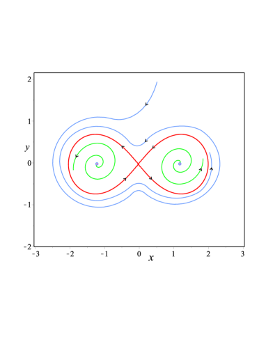
Figure 1: The phase portrait of (3.26) with $b(x,y)=-\nabla V(x,y)-\Theta(x,y)$.

Proof.

It is easy to see that

$$\lim_{|(x,y)|\rightarrow\infty}V(I(x,y))=\infty.$$ (3.28)

Since $\nabla V(I)$ and $\Theta(x,y)$ are orthogonal, the derivative of the function $V(I(x,y))$ along a solution is

$$\dot{V}=-|\nabla V(I)|^{2}.$$ (3.29)

(3.28) and (3.29) imply that all positive trajectories for (3.26) are bounded. The LaSalle invariance principle deduces that for any $p\in\mathbb{R}^{2}$,

$$\omega(p)\subset\{(x,y):\nabla V(I)=0\}=L\cup\{P^{+},P^{-}\}.$$

In particular, the equilibria for (3.26) is contained in $L\cup\{P^{+},P^{-}\}.$ It is easy to calculate that there uniquely exists an equilibrium on $L$, which is the origin $O$, and that the other equilibria are $P^{+}$ and $P^{-}$. It is not hard to get that

$$\begin{array}[]{cc}Db(0,0)=\left(\begin{array}[]{cc}0&-8\\ -8&0\\ \end{array}\right),&Db(\sqrt{2},0)=Db(-\sqrt{2},0)=16\left(\begin{array}[]{cc}\frac{20}{17^{\frac{7}{4}}}&-\frac{5}{17^{\frac{11}{8}}}\\[5.0pt] \frac{5}{17^{\frac{11}{8}}}&\frac{20}{17^{\frac{7}{4}}}\\ \end{array}\right).\\ \end{array}$$

This implies that $(0,0)$ is a saddle point and $(\pm\sqrt{2},0)$ are unstable focus. Combining the LaSalle invariance principle and the Poincaré-Bendixson Theorem, we can obtain the $\omega$-limit set of each trajectory for (3.26), as shown in Figure 1.

By estimation, we can obtain the following inequalities:

$$|\frac{\partial b_{i}(x,y)}{\partial x}|,\ |\frac{\partial b_{i}(x,y)}{\partial y}|\leq 130\sqrt[4]{8},\ r\geq 4,\ i=1,2,$$

where $r=\sqrt{x^{2}+y^{2}}$. Therefore, $b(x,y)$ is a globally Lipschitz function. This completes the proof. ∎

Now we consider perturbed system of (3.26) driven by Brownian motion:

$$\left\{\begin{aligned} dx&=b_{1}(x,y)dt+\epsilon[\sigma_{11}(x,y)dW_{t}^{1}+\sigma_{12}(x,y)dW_{t}^{2}],\\ dy&=b_{2}(x,y)dt+\epsilon[\sigma_{21}(x,y)dW_{t}^{1}+\sigma_{22}(x,y)dW_{t}^{2}],\end{aligned}\right.$$ (3.30)

where $\sigma_{ij}(i,j\in\{1,2\})$ satisfies global Lipschitz condition, which implies that there exist nonnegative constants $C_{1}$, $C_{2}$ such that

$$|a_{ij}(x,y)|\leq C_{1}|(x,y)|^{2}+C_{2}\leq C_{1}r^{2}+C_{2},\>\>\textrm{for}\>\>i,j=1,2,$$

where $a_{ij}(x,y)=\displaystyle\sum_{k=1}^{2}\sigma_{ik}(x,y)\sigma_{jk}(x,y)$.

Theorem 3.7.

Suppose that $\sigma_{ij}(i,j\in\{1,2\})$ satisfies global Lipschtiz condition,

(i) if $C_{1}=0$, then for any $\epsilon$, the system (3.30) admits at least one stationary measure $\mu^{\epsilon}$;

(ii) if $C_{1}>0$, then the system (3.30) possesses at least one stationary measure $\mu^{\epsilon}$ for $0<\epsilon<\frac{1}{8\sqrt{26C_{1}}}$.

If, in addition, the diffusion matrix $a(x,y)$ is positively definite everywhere, then for a given $\epsilon$ as above, the stationary measure $\mu^{\epsilon}$ is unique, and $\mu^{\epsilon}\overset{w}{\rightarrow}\delta_{O}(\cdot)$ as $\epsilon\rightarrow 0$, where $\delta_{O}(\cdot)$ denotes the Dirac measure at the saddle $O$.

Proof.

In fact, from the above inequalities one can see that for $r>4$,

$$|\frac{\partial^{2}V}{\partial x^{2}}|,|\frac{\partial^{2}V}{\partial y^{2}}|,|\frac{\partial^{2}V}{\partial y\partial x}|\leq 104\sqrt{2},\ |\nabla V(x,y)|^{2}\geq\frac{r^{2}}{4\sqrt{2}},$$

and

$$\mathcal{L}^{\epsilon}V(x,y)\leq-[\frac{1}{4\sqrt{2}}-208\sqrt{2}C_{1}\epsilon^{2}]r^{2}+208\sqrt{2}C_{2}\epsilon^{2}\rightarrow-\infty\ {\rm as}\ r\rightarrow\infty.$$

Applying the Khasminskii Theorem 3.3, we conclude that there is at least one stationary measure for (3.30) if $0<\epsilon<\frac{1}{8\sqrt{26C_{1}}}$ with $C_{1}>0$ or all $\sigma_{ij}(x,y)$ are bounded on the plane, and that this stationary measure is unique if $a(x,y)$ is positively definite everywhere.

In (i) and (ii), from the Tightness Criterion it follows that the set of stationary measures $\{\mu^{\epsilon}:\epsilon\in(0,\epsilon_{0}]\}$ is tight. Thus the Prohorov theorem implies that any sequence $\{\mu^{\epsilon_{i}}\}$ of stationary measures with $\epsilon_{i}\rightarrow 0$ contains a weak convergent subsequence. Let $\mu$ be any weak limit measure. Then Theorem 2.1 deduces that ${\rm supp}(\mu)\subset B(\Phi)$. However, in view of Proposition 3.3, $B(\Phi)=\{O,P^{+},P^{-}\}$, which implies that ${\rm supp}(\mu)\subset\{O,P^{+},P^{-}\}$.

Finally, we show that $\mu(\{P^{+},P^{-}\})=0$. Since matrix $Db(P^{+})$ has all eigenvalues with positive real parts. Thus there exists a positive definite matrix $B$ satisfying

$$\big{(}Db(P^{+})\big{)}^{T}B+B\big{(}Db(P^{+})\big{)}=I$$

Let $\tilde{V}^{+}(z)=(z-P^{+})^{T}B(z-P^{+})$, where $z=(x,y)$. It is easy to see that there exists a neighborhood $\mathcal{U}:=B_{\delta}(P^{+})$ of $P^{+}$ such that $\langle\nabla\tilde{V}^{+},b\rangle>0$ on $\mathcal{U}\setminus\{P^{+}\}$ (e.g. see [26]). We denote $\rho_{M}:=\displaystyle\sup_{(x,y)\in\mathcal{U}}\tilde{V}^{+}(x,y)$ (called essential upper bound of $\tilde{V}^{+}$). Then

$$\begin{split}\mathcal{L}^{\epsilon}\tilde{V}^{+}(x,y)=&\langle b(x,y),\nabla\tilde{V}^{+}(x,y)\rangle\\ &+\frac{\epsilon^{2}}{2}[a_{11}(x,y)\frac{\partial^{2}V}{\partial x^{2}}+2a_{12}(x,y)\frac{\partial^{2}V}{\partial y\partial x}+a_{22}(x,y)\frac{\partial^{2}V}{\partial y^{2}}]\\ \geq&\frac{\epsilon^{2}}{2}[a_{11}(x,y)b_{11}+2a_{12}(x,y)b_{12}+a_{22}(x,y)b_{22}]\\ \geq&\widetilde{m}\epsilon^{2}=:\gamma>0,\quad\forall(x,y)\in\mathcal{U}.\end{split}$$ (3.31)

We used here the fact that $B$ is positively definite and $A(x,y)$ is positively definite on $\bar{B}_{\delta}(P^{+})$. It follows from (3.31) that $\tilde{V}^{+}$ is an anti-Lyapunov function with respect to (3.30) in $B_{\delta}(P^{+})$ with anti-Lyapunov constant $\widetilde{m}\epsilon^{2}$ and essential lower bound $\rho_{m}=0$ (e.g. see [29, Definition 2.2]). It is obviously

$$\nabla\tilde{V}^{+}(x,y)= \big{(}2b_{11}(x-\sqrt{2})+2b_{12}y,2b_{12}(x-\sqrt{2})+2b_{22}y\big{)}$$

$$\neq 0,\quad\forall(x,y)\in\big{(}\tilde{V}^{+}\big{)}^{-1}(\rho)\>\>\>\textrm{for}\>a.e.\>\rho\in[0,\rho_{M}),$$ (3.32)

where $\big{(}\tilde{V}^{+}\big{)}^{-1}(\rho)=\{(x,y)\in\mathcal{U}:\tilde{V}^{+}(x,y)=\rho\}$. Note that

$$\begin{split}&\frac{\epsilon^{2}}{2}[a_{11}(x,y)(\frac{\partial\tilde{V}^{+}}{\partial x})^{2}+2a_{12}(x,y)\frac{\partial\tilde{V}^{+}}{\partial x}\frac{\partial\tilde{V}^{+}}{\partial y}+a_{22}(x,y)(\frac{\partial\tilde{V}^{+}}{\partial y})^{2}]\\ \leq&\frac{\epsilon^{2}}{2}\|A(x,y)\||\big{(}\frac{\partial\tilde{V}^{+}}{\partial x}(x,y),\frac{\partial\tilde{V}^{+}}{\partial y}(x,y)\big{)}|^{2}\\ \leq&\displaystyle\sup_{(x,y)\in B_{\delta}(P^{+})}\|A(x,y)\|\widetilde{M}_{0}|\tilde{V}^{+}(x,y)|\epsilon^{2}\\ =:&\widetilde{M}\rho\epsilon^{2}=:H(\rho),\quad(x,y)\in\big{(}\tilde{V}^{+}\big{)}^{-1}(\rho)\>\>\>\textrm{for}\>\>\rho\in[0,\rho_{M}).\end{split}$$ (3.33)

Without loss of generality, we may assume $\mu^{\epsilon}(\mathcal{U})>0$ for each $\epsilon>0$. It is easy to verify that $\tilde{\mu}^{\epsilon}(\cdot)=\frac{\mu^{\epsilon}|_{\mathcal{U}}(\cdot)}{\mu^{\epsilon}(\mathcal{U})}$ is a stationary measure in $\mathcal{U}$, by a regularity result on stationary measure in [6], we have known that $\tilde{\mu}^{\epsilon}$ admits a positive density function $\tilde{u}\in W^{1,p}_{loc}(\mathcal{U})$. Let $\Omega_{\rho}=\{(x,y)\in\mathcal{U}:\tilde{V}^{+}(x,y)<\rho\}$, $\Omega^{*}_{\rho}=\Omega_{\rho}\cup\big{(}\tilde{V}^{+}\big{)}^{-1}(\rho)$ for each $\rho\in[0,\rho_{M})$. The regularity implies that $\tilde{\mu}^{\epsilon}(\Omega^{*}_{\rho_{m}})=\tilde{\mu}^{\epsilon}(\{P^{+}\})=0$. Measure estimate theorem in Huang-Ji-Liu-Yi [27, Theorem B a)] asserts that for any $\rho_{0}\in(0,\rho_{M})$,

$$\begin{split}\tilde{\mu}^{\epsilon}(\Omega_{\rho})=\tilde{\mu}^{\epsilon}(\Omega_{\rho}\setminus\Omega^{*}_{\rho_{m}})\geq&\tilde{\mu}^{\epsilon}(\Omega_{\rho_{0}}\setminus\Omega^{*}_{\rho_{m}})e^{\gamma\int_{\rho_{0}}^{\rho}\frac{1}{H(t)}dt}\\ =&\tilde{\mu}^{\epsilon}(\Omega_{\rho_{0}})e^{\widetilde{m}\epsilon^{2}\int_{\rho_{0}}^{\rho}\frac{1}{\widetilde{M}\epsilon^{2}t}dt}\\ =&\tilde{\mu}^{\epsilon}(\Omega_{\rho_{0}})e^{\frac{\widetilde{m}}{\widetilde{M}}\int_{\rho_{0}}^{\rho}\frac{1}{t}dt},\quad\rho\in(\rho_{0},\rho_{M}),\end{split}$$

This is,

$$\mu^{\epsilon}(\Omega_{\rho_{0}})\leq\mu^{\epsilon}(\Omega_{\rho})e^{-\frac{\widetilde{m}}{\widetilde{M}}\int_{\rho_{0}}^{\rho}\frac{1}{t}dt}\leq e^{-\frac{\widetilde{m}}{\widetilde{M}}\int_{\rho_{0}}^{\rho}\frac{1}{t}dt},\quad\rho\in(\rho_{0},\rho_{M}).$$

Since $\mu^{\epsilon}\xlongrightarrow{w}\mu$ as $\epsilon\rightarrow 0$, and $\Omega_{\rho_{0}}$ is an open set, we have

$$\mu(\Omega_{\rho_{0}})\leq e^{-\frac{\widetilde{m}}{\widetilde{M}}\int_{\rho_{0}}^{\rho}\frac{1}{t}dt}.$$

Finally, letting $\rho_{0}\rightarrow 0$, we obtain $\mu(\{P^{+}\})=0$. Analogously, we can verify that $\mu(\{P^{-}\})=0$. We conclude that $\mu=\delta_{O}(\cdot)$, that is, $\mu^{\epsilon}\overset{w}{\rightarrow}\delta_{O}(\cdot)$ as $\epsilon\rightarrow 0$. ∎

Remark 6.

From the above arguments, we have obtained that if the system ${\rm(\ref{unds})}$ is driven by Brownian motion and the diffusion matrix is positively definite everywhere, then any limiting measure is $\delta_{O}$. However, if we get rid of nondegenerate condition for the diffusion matrix , then it is possible for limiting measure to be either $\delta_{P^{+}}$ or $\delta_{P^{-}}$ from Proposition 3.2. The problem is whether or not such result still holds if it is driven by Lévy process, we can only get that the limiting measure is supported in $\{O,P^{+},P^{-}\}$.

Example 3 is complete. $\qquad\qquad\qquad\qquad\qquad\qquad\qquad\qquad\qquad\qquad\quad\Box$

Example 4 (May-Leonard System with a Noise Perturbation).

Consider the May-Leonard system with a white noise perturbation:

$$\left\{\begin{array}[]{l}dy_{1}=y_{1}(1-y_{1}-\beta y_{2}-\gamma y_{3})dt+\epsilon y_{1}\circ dW_{t},\\ dy_{2}=y_{2}(1-y_{2}-\beta y_{3}-\gamma y_{1})dt+\epsilon y_{2}\circ dW_{t},\\ dy_{3}=y_{3}(1-y_{3}-\beta y_{1}-\gamma y_{2})dt+\epsilon y_{3}\circ dW_{t},\\ \end{array}\right.$$ (3.34)

where $\circ$ denotes the Stratonovich stochastic integral, $\beta,\ \gamma>0$ and $\epsilon$ denotes noise intensity.

Recalling from [8], we have the following Stochastic Decomposition Formula:

$$\Phi^{\epsilon}(t,\omega,y)=g^{\epsilon}(t,\omega,g_{0})\Phi^{0}(\int_{0}^{t}g^{\epsilon}(s,\omega,g_{0})ds,\frac{y}{g_{0}}),$$ (3.35)

where $\Phi^{\epsilon},\ \Phi^{0}$ are the solutions of (3.34) and the corresponding deterministic system without noise, respectively, and $g^{\epsilon}$ is the solution of stochastic Logistic equation

$$dg=g(1-g)dt+\epsilon g\circ dW_{t}.$$ (3.36)

In order to obtain the stationary properties for (3.34) in detail, we need the asymptotic properties for deterministic flow $\Phi^{0}$. It is well-known from Hirsch [24] that the flow $\Phi^{0}$ admits an invariant surface $\Sigma$ (called carrying simplex), homeomorphic to the closed unit simplex $\Delta^{2}=\{y\in\mathbb{R}^{3}_{+}:\sum_{i}y_{i}=1\}$ by radial projection, such that every trajectory in $\mathbb{R}^{3}_{+}\setminus\{O\}$ is asymptotic to one in $\Sigma$. So we will draw phase portraits on $\Sigma$ (see Table LABEL:biao0).

It is easy to see that $\Phi^{0}$ always possesses equilibria: the origin $O(0,0,0)$, three axial equilibria $R_{1}(1,0,0),\ R_{2}(0,1,0),\ R_{3}(0,0,1)$ and the unique positive equilibrium $P=\frac{1}{1+\beta+\gamma}(1,1,1)$. $\Phi^{0}$ has planar equilibria: $R_{12}=\frac{1}{1-\beta\gamma}(1-\beta,1-\gamma,0)$, $R_{23}=\frac{1}{1-\beta\gamma}(0,1-\beta,1-\gamma)$, $R_{31}=\frac{1}{1-\beta\gamma}(1-\gamma,0,1-\beta)$ if and only if $(1-\beta)(1-\beta\gamma)>0$, $(1-\gamma)(1-\beta\gamma)>0$. The classification for the flow $\Phi^{0}$ on the carrying simplex $\Sigma$ is summarized in Table LABEL:biao0.

Table 1: The classification for the flow $\Phi^{0}$ on $\Sigma$

Parameter conditions	Equilibria	Phase Portrait
a: $0<\beta,\gamma<1$	$O,R_{1},R_{2},R_{3},R_{12},R_{13},R_{23},P$
b: (i) $\beta+\gamma<2$ (ii) $\beta\geq 1,\gamma<1$ or  $\gamma\geq 1,\beta<1$	$O,R_{1},R_{2},R_{3},P$
c: (i) $\beta+\gamma=2$ (ii)  $\beta,\gamma\neq 1$	$O,R_{1},R_{2},R_{3},P$
d: (i)  $\beta+\gamma>2$ (ii)  $\gamma>1,\beta\leq 1$ or  $\gamma\leq 1,\beta>1$	$O,R_{1},R_{2},R_{3},P$
e: $\beta,\gamma>1$	$O,R_{1},R_{2},R_{3},R_{12},R_{13},R_{23},P$
f: $\beta=\gamma=1$	$\forall x\in\Sigma\cup\{O\}$

Table 1: (continued)

Set by $\omega(z)$ the $\omega-$limit set for the trajectory $\Phi^{0}(t,z)$. Then it follows from Table LABEL:biao0 that any $\omega(z)$ is either an equilibrium, or a closed orbit, or heterclinic cycle. Define

$$\mathcal{A}(\omega(z)):=\{y\in\mathbb{R}^{3}_{+}:\lim_{t\to\infty}\mathrm{dist}(\Phi^{0}(t,y),\omega(z))=0\}$$

to be the attracting domain for $\omega(z)$, and let $\mathcal{A}_{\Sigma}(\omega(z))$ denote the attracting domain for $\omega(z)$ on $\Sigma$, which can be derived from Table LABEL:biao0 for each case. It follows from [9, Proposition 4.13] that any pair of points on $L(y):=\{\lambda y:\lambda>0\}$ have the same $\omega-$limit set. We can obtain the attracting domain for $\omega(z)$ as follows

$$\mathcal{A}(\omega(z))=\bigcup\{L(y):y\in\mathcal{A}_{\Sigma}(\omega(z))\}.$$ (3.37)

Together with Table LABEL:biao0 and (3.37), we can obtain the attracting domains for an equilibrium, a closed orbit, or the heterclinic cycle, respectively.

Using the Stochastic Decomposition Formula (3.35), we have shown that Probability Convergence (2.1) holds, that is, $\Phi^{\epsilon}$ converges to $\Phi^{0}$ as $\epsilon\rightarrow 0$ in probability (see [8, Proposition 1]) and that for any $y\neq O$, the probability measures

$$P_{T}(\cdot,y):=\frac{1}{T}\int_{0}^{T}P(t,y,\cdot)dt,\ \ T>0$$ (3.38)

is tight, and has at least a limiting measure $\nu_{y}^{\epsilon}$ in weak sense, which is a stationary measure for (3.34) (see [8, Theorem 8]). Now denote by

$$\mathcal{M}_{S}(\epsilon_{0}):=\{\nu_{y}^{\epsilon}:{\rm for\ all}\ 0<\epsilon\leq\epsilon_{0},\ y\in\mathbb{R}^{3}_{+}\}$$

all the stationary measures obtained in a manner just stated, which is tight (see [8, Proposition 2]) and produced by all solutions from $\Sigma\cup\{O\}$ (see [8, Theorem 12]).

It is not difficult to see that stochastic Logistic equation (3.36) has a unique nontrivial stationary solution $u^{\epsilon}(\theta_{t}\omega)$ where $\theta_{t}$ is the metric dynamical system generated by Brownian motion. It follows from the Stochastic Decomposition Formula that $u^{\epsilon}(\theta_{t}\omega)Q$ is a stationary solution of (3.34) for any equilibrium $Q\in\mathcal{E}$ (see [8, Theorem 5]), whose distribution measure, denoted by $\mu^{\epsilon}_{Q}$, defines an ergodic stationary measure for (3.34) (see [8, Theorem 7]). In addition, for each $y\in\mathcal{A}(Q)$, $P(t,y,\cdot){\rightarrow}\mu^{\epsilon}_{Q}$ weakly as $t\rightarrow\infty$, and

$$\lim_{t\rightarrow\infty}P(t,y,A)=\mu^{\epsilon}_{Q}(A),\ {\rm for\ any}\ A\in\mathcal{B}(\mathbb{R}_{+}^{3}).$$ (3.39)

This shows

$$\mathcal{M}_{S}(\epsilon_{0})=\{\mu^{\epsilon}_{Q}:Q\in\mathcal{E},0<\epsilon\leq\epsilon_{0}\}$$

in the cases a, b, e, f of Table LABEL:biao0.

In the case c of Table LABEL:biao0, the carrying simplex is full of periodic orbits $\Gamma(h)\ (0<h\leq\frac{1}{27})$:

$$\left\{\begin{array}[]{l}y_{1}+y_{2}+y_{3}=1,\\ \vskip 6.0pt plus 2.0pt minus 2.0pt\cr y_{1}y_{2}y_{3}=h,\\ \end{array}\right.$$

whose attracting domain is the invariant cone surface $\Lambda(h):$

$$\ \frac{y_{1}y_{2}y_{3}}{(y_{1}+y_{2}+y_{3})^{3}}=h,\ 0<h\leq\frac{1}{27}.$$

Then there exists a unique ergodic nontrivial stationary measure $\nu_{h}^{\epsilon}$ supporting on the cone surface $\Lambda(h)$ (see [8, Theorem 20]). Hence,

$$\mathcal{M}_{S}(\epsilon_{0})=\{\nu_{h}^{\epsilon}:0<h\leq\frac{1}{27},0<\epsilon\leq\epsilon_{0}\}\bigcup\{\mu_{Q}^{\epsilon}:Q\in\mathcal{E},0<\epsilon\leq\epsilon_{0}\}.$$

The above discusses illustrate a uniform characteristic: the time average measure (3.38) of transition probability function for each solution weakly converges to an ergodic stationary measure for (3.34) on the attracting domain of the $\omega$-limit set of the orbit for $\Phi^{0}$ through the same initial point. But case d is quite different. If $y\in{\rm Int}\mathbb{R}_{+}^{3}\backslash\overline{L(P)}$, the corresponding time average measure (3.38) of transition probability function has infinite weak limit points, which are not ergodic (see [8, Theorem 23 and Appendix B]).

Applying Theorem 2.1, we conclude that

Theorem 3.8.

1. For any equilibrium $Q\in\mathcal{E}$, $\mu^{\epsilon}_{Q}(\cdot)\stackrel{{\scriptstyle w}}{{\rightarrow}}\delta_{Q}(\cdot)$ as $\epsilon\rightarrow 0$, which is valid to the cases a, b, e, f.

2. For the case c, $\nu_{h}^{\epsilon}$ converges weakly to the Haar measure on the closed orbit $\Gamma(h)$ as $\epsilon\rightarrow 0,0<h\leq\frac{1}{27}.$

3. For the case d, if $\mu^{i}:=\nu_{y}^{\epsilon^{i}}\in\mathcal{M}_{S}(\epsilon_{0}),\ i=1,2,\cdots,$ satisfying $\epsilon^{i}\rightarrow 0$ and $\mu^{i}\stackrel{{\scriptstyle w}}{{\rightarrow}}\mu$ as $i\rightarrow\infty$, then $\mu(\{R_{1},R_{2},R_{3}\})=1.$

Remark 7.

The Birkhoff center in Example ${\rm(\ref{unds})}$ consists of the origin (saddle) and strongly unstable foci $\{P^{+},P^{-}\}$. Relatively, the orgin $O$ is more stable than $\{P^{+},P^{-}\}$. So all limiting measures support at the origin in the case that the diffusion matrix is nondegenerate. The Birkhoff center for the flow $\Phi^{0}$ on $\Sigma$ is composed of $P$ (which is strongly repelling on $\Sigma$) and three saddles $\{R_{1},R_{2},R_{3}\}$, which are relatively more stable than $P$ and supported by all limiting measures determined by those solutions with initial points on $\Sigma$. Nevertheless, if the drift system is Morse-Smale and the diffusion matrix is positively definite everywhere, then we conjecture that all limiting measures will support at either stable equilibrium or stable periodic orbit.

Example 4 is complete. $\qquad\qquad\qquad\qquad\qquad\qquad\qquad\qquad\qquad\qquad\quad\Box$

4 Applications to SPDEs

Although our main result can be applied to many SPDEs, we prefer to apply it to stochastic reaction-diffusion equations, stochastic $2D$ Navier-Stokes equations and stochastic Burgers type equations driven by Brownian motions or Lévy process.

4.1 Stochastic reaction diffusion equation with a polynomial nonlinearity

Let $\Lambda\subset\mathbb{R}^{n}$ be a bounded domain with smooth boundary $\partial\Lambda$ and let $g$ be a polynomial of odd degree with negative leading coefficient

$$g(u)=\displaystyle\sum_{i=0}^{2k-1}a_{i}u^{i},\quad a_{2k-1}<0.$$ (4.1)

Consider the following initial boundary value problem:

$$\left\{\begin{array}[]{l}\frac{\partial u}{\partial t}=\Delta u+g(u),\ x\in\Lambda,\ t>0,\\ u(x,t)=0,\ x\in\partial\Lambda,\ t\geq 0,\\ u(x,0)=\varphi\in L^{2}(\Lambda).\end{array}\right.$$ (4.2)

Then by Temam [47, p.84 Theorem III.1.1], equation (4.2) has a unique solution $u(x,t;\varphi)\in L^{2}(\Lambda)$. Therefore we can define a semigroup $T(t)$ on $L^{2}(\Lambda)$: $T(t):\varphi\in L^{2}(\Lambda)\mapsto u(t;\varphi)\in H^{1}_{0}(\Lambda)$. Thanks to [47, p.88 Theorem III.1.2], equation (4.2) has a global attractor $\mathcal{A}_{L^{2}(\Lambda)}$ which is bounded in $H^{1}_{0}(\Lambda)$, compact and connected in $L^{2}(\Lambda)$. We have that for any $\varphi\in H^{1}_{0}(\Lambda)$, $\{u(x,t;\varphi)\}_{t\geq 0}$ is bounded in $H_{0}^{1}(\Lambda)$. Furthermore, since $-\Delta$ has compact resolvent, trajectory $\{u(x,t;\varphi)\}_{t\geq 0}$ has a compact closure. And let

$$V(\varphi)=\int_{\Lambda}\big{(}\frac{1}{2}|\nabla\varphi|^{2}-G(\varphi)\big{)}dx,\ G(u)=\int_{0}^{u}g(\xi)d\xi,\quad\varphi\in H_{0}^{1}(\Lambda),$$

then

$$\frac{d}{dt}V(u(x,t;\varphi)) =\frac{d}{dt}\int_{\Lambda}\big{(}\frac{1}{2}|\nabla u|^{2}-G(u)\big{)}dx$$

$$=\int_{\Lambda}\big{(}\frac{1}{2}2\nabla u\cdot\nabla\frac{\partial u}{\partial t}-g(u)\frac{\partial u}{\partial t}\big{)}dx$$

$$=-\int_{\Lambda}\big{(}(\Delta u+g(u))\frac{\partial u}{\partial t}\big{)}dx$$

$$=-\int_{\Lambda}\big{(}\frac{\partial u}{\partial t}\big{)}^{2}dx\leq 0$$

where we have used the Green formula and boundary condition in the third equality. Finally, by LaSalle’s invariance principle, the $\omega$-limit set $\omega(\varphi)$ is contained in the equilibrium set of $T(t)$ for any $\varphi\in H_{0}^{1}(\Lambda)$, this is, $u(x,t;\varphi)=\varphi$ satisfies the following boundary value problem

$$\left\{\begin{array}[]{l}\Delta\varphi+g(\varphi)=0,\ x\in\Lambda,\\ \varphi(x)=0,\ x\in\partial\Lambda.\end{array}\right.$$

This implies that all solutions for (4.2) are convergent to the equilibrium points.

Proposition 4.1.

The Birkhoff center for ${\rm(\ref{nonpoly})}$ is the equilibrium set $\mathcal{E}$.

Now let us consider the noise perturbation system of reaction diffusion equation, such as (4.2).

Consider the following stochastic reaction diffusion equation in $\Lambda$ with Dirichlet boundary conditions:

$$\left\{\begin{aligned} &dX(t,x)=\nu\Delta X(t,x)dt+g(x,X(t,x))dt+\epsilon\sigma(x,X(t,x))dW(t),\\ &X(t,x)=0,\ x\in\partial\Lambda,\ t>0,\\ &X(0)=h\in L^{2}(\Lambda).\end{aligned}\right.$$ (4.3)

Here $\nu>0$, $g:\Lambda\times\mathbb{R}\rightarrow\mathbb{R}$ and $\sigma:\Lambda\times\mathbb{R}\rightarrow l^{2}$ are two measurable functions. $W(t)=(W_{k}(t))_{k\in\mathbb{N}}$ is a sequence of independent one dimensional standard Brownian motions on some filtered probability space $(\Omega,\mathcal{F},\{\mathcal{F}_{t}\}_{t\geq 0},\mathbb{P})$.

For $p\geq 1$, let $L^{p}(\Lambda)$ be the usual $L^{p}$-space over $\Lambda$ with the standard norm $\|\cdot\|_{p}$. For $m\in\mathbb{N}$, let $\mathbb{H}^{m}_{0}(\Lambda)$ be the usual $m$-order Sobolev space over $\Lambda$ with Dirichlet boundary conditions, and its norm is denoted by $\|\cdot\|_{2,m}$. Denote $\mathbb{H}^{-m}(\Lambda)$ be the dual space of $\mathbb{H}^{m}_{0}(\Lambda)$. Notice that the following Poincaré inequality holds: for some $\lambda_{\Lambda}>0$,

$$\lambda_{\Lambda}\|u\|^{2}_{2}\leq\|\nabla u\|^{2}_{2},\ \ u\in\mathbb{H}^{1}_{0}(\Lambda).$$

Let $V:=\mathbb{H}^{1}_{0}(\Lambda)$ and denote by $\|u\|_{V}:=\|\nabla u\|_{2}$.

Now we identify the Hilbert space $H:=L^{2}(\Lambda)$ with itself by the Riesz representation, and set for $q\geq 2$,

$$V_{q}:=\mathbb{H}^{1}_{0}(\Lambda)\cap L^{q}(\Lambda),\ \ \ \ \ V^{*}_{q}=\mathbb{H}^{-1}(\Lambda)+L^{q^{*}}(\Lambda),$$

where $q^{*}:=q/(q-1)$. For any $u\in V_{q}$ and $w=w_{1}+w_{2}\in\mathbb{H}^{-1}(\Lambda)+L^{q^{*}}(\Lambda)$, we have

$$\langle u,w\rangle_{V_{q},V^{*}_{q}}=\langle u,w_{1}\rangle_{\mathbb{H}^{1}_{0},\mathbb{H}^{-1}}+\langle u,w_{2}\rangle_{L^{q}(\Lambda),L^{q^{*}}(\Lambda)}.$$

In what follows, we consider the evolution triple

$$V_{q}\subset H\subset V^{*}_{q}.$$

Assume that

• There exist $q\geq 2$, $c_{i}>0,i=1,2,3,4$ and $h_{1}\in L^{1}(\Lambda)$, $h_{2}\in L^{q^{*}}(\Lambda)$ such that for all $u,u^{\prime}\in\mathbb{R}$ and $x\in\Lambda$,

  $$(u-u^{\prime})(g(x,u)-g(x,u^{\prime}))\leq c_{1}|u-u^{\prime}|^{2},$$

  $$ug(x,u)\leq-c_{2}|u|^{q}+c_{3}|u|^{2}+h_{1}(x),$$

  $$|g(x,u)|\leq c_{4}|u|^{q-1}+h_{2}(x),$$

  and the mapping $u\mapsto g(x,u)$ is continuous.

• There exist $c_{5},c_{6}>0$ and $h_{3}\in L^{1}(\Lambda)$ such that for all $u,u^{\prime}\in\mathbb{R}$ and $x\in\Lambda$,

  $$\|\sigma(x,u)-\sigma(x,u^{\prime})\|^{2}_{l^{2}}\leq c_{5}|u-u^{\prime}|^{2},$$

  and

  $$\|\sigma(x,u)\|^{2}_{l^{2}}\leq c_{6}|u|^{2}+h_{3}(x),$$

where $l^{2}$ be the Hilbert space of all square summable sequences of real numbers. By Theorem 3.2 in [37] or Theorem 3.6 in [51], under (C1)-(C2), for any $p\geq 1$ and $h\in L^{2p}(\Omega,\mathcal{F}_{0},\mathbb{P};L^{2}(\Lambda))$, there exists a unique $L^{2}(\Lambda)$-valued $\mathcal{F}_{t}$-adapted process $X^{\epsilon,h}$ with

$$X^{\epsilon,h}\in C_{loc}([0,\infty),L^{2}(\Lambda))\cap L^{2}_{loc}([0,\infty),V)\cap L^{q}_{loc}([0,\infty),L^{q}(\Lambda)),\ \ \mathbb{P}\text{-a.s.}$$

and equation (4.3) holds in $V^{*}_{q}$. Moreover, we can obtain

Lemma 4.1.

Assume (C1)-(C2) hold, and $q>2$ or $q=2,\nu+\frac{c_{2}-c_{3}}{\lambda_{\Lambda}}>0$. Then there exists $\epsilon_{0}>0$ such that for any $\epsilon\in(0,\epsilon_{0}]$,

$$\mathbb{E}\big{(}\sup_{t\in[0,T]}\|X^{\epsilon,h}(t)\|^{2}_{2}\big{)}+\mathbb{E}\big{(}\int_{0}^{T}\|X^{\epsilon,h}(t)\|^{2}_{V}dt\big{)}\leq C\big{(}\mathbb{E}(\|h\|^{2}_{2})+T\big{)}.$$ (4.4)

Remark 8.

By Fubini’s Theorem and (4.4), we have

$$\int_{0}^{T}\mathbb{E}\Big{(}\|X^{\epsilon,h}(t)\|^{2}_{V}\Big{)}dt<\infty.$$

This implies that there exists $\mathcal{T}_{0}\in\mathcal{B}([0,T])$ with zero Lebesgue measure such that

$$\mathbb{E}\Big{(}\|X^{\epsilon,h}(t)\|^{2}_{V}\Big{)}<\infty,\ \ \ t\in[0,T]\setminus\mathcal{T}_{0}.$$

Hence for any $t\in[0,T]\setminus\mathcal{T}_{0}$, there exists $\Omega_{t}\in\mathcal{F}$ with $\mathbb{P}(\Omega_{t})=1$ such that

$$X^{\epsilon,h}(t,\omega)\in V,\ \ \omega\in\Omega_{t}.$$

Proof.

Denote by $(L_{2}(l^{2},H),\|\cdot\|_{l^{2},H})$ the Hilbert space of all Hilbert-Schmidt operators for $l^{2}$ to $H$.

By Itô’s formula,

$$\|X^{\epsilon,h}(t)\|^{2}_{2}+2\nu\int_{0}^{t}\|X^{\epsilon,h}(s)\|^{2}_{V}ds\$$

$$= \|h\|^{2}_{2}+2\int_{0}^{t}\langle X^{\epsilon,h}(s),g(x,X^{\epsilon,h}(s))\rangle_{H,H}ds$$

$$+2\epsilon\int_{0}^{t}\langle X^{\epsilon,h}(s),\sigma(x,X^{\epsilon,h}(s))dW(s)\rangle_{H,H}$$

$$+\epsilon^{2}\int_{0}^{t}\|\sigma(x,X^{\epsilon,h}(s))\|^{2}_{l^{2},H}ds$$

$$:= I^{\epsilon}_{1}+I^{\epsilon}_{2}(t)+I^{\epsilon}_{3}(t)+I^{\epsilon}_{4}(t).$$

For $I^{\epsilon}_{3}$, by (C2),

$$\begin{split}&\mathbb{E}\Big{(}\sup_{t\in[0,T]}|I^{\epsilon}_{3}(t)|\Big{)}\\ \leq&2\epsilon\mathbb{E}\Big{(}\int_{0}^{T}\|X^{\epsilon,h}(t)\|^{2}_{2}\|\sigma(x,X^{\epsilon,h}(t))\|^{2}_{l^{2},H}dt\Big{)}^{1/2}\\ \leq&2\epsilon\mathbb{E}\Big{(}\sup_{t\in[0,T]}\|X^{\epsilon,h}(t)\|^{2}_{2}\Big{)}+2\epsilon\mathbb{E}\Big{(}\int_{0}^{T}\|\sigma(x,X^{\epsilon,h}(t))\|^{2}_{l^{2},H}dt\Big{)}\\ \leq&2\epsilon\mathbb{E}\Big{(}\sup_{t\in[0,T]}\|X^{\epsilon,h}(t)\|^{2}_{2}\Big{)}+2\epsilon c_{6}\mathbb{E}\Big{(}\int_{0}^{T}\|X^{\epsilon,h}(t)\|^{2}_{2}dt\Big{)}+2\epsilon T\|h_{3}\|_{1}\\ \leq&2\epsilon\mathbb{E}\Big{(}\sup_{t\in[0,T]}\|X^{\epsilon,h}(t)\|^{2}_{2}\Big{)}+\frac{2\epsilon c_{6}}{\lambda_{\Lambda}}\mathbb{E}\Big{(}\int_{0}^{T}\|X^{\epsilon,h}(t)\|^{2}_{V}dt\Big{)}+2\epsilon T\|h_{3}\|_{1}.\end{split}$$ (4.5)

For $I^{\epsilon}_{4}$, applying (C2) again, we have

$$\mathbb{E}\Big{(}I^{\epsilon}_{4}(T)\Big{)}\leq\frac{\epsilon^{2}c_{6}}{\lambda_{{\Lambda}}}\mathbb{E}\Big{(}\int_{0}^{T}\|X^{\epsilon,h}(s)\|^{2}_{V}ds\Big{)}+\epsilon^{2}T\|h_{3}\|_{1}.$$ (4.6)

$I^{\epsilon}_{2}$ will be estimated according to two cases.

• The case $q>2$ or $q=2,c_{2}-c_{3}\geq 0$.

  By (C1), it is easy to see that there exist $\kappa\geq 0$ and $\tilde{h}_{1}\in L^{1}(\Lambda)$ such that

  $$ug(x,u)\leq-\kappa|u|^{q}+\tilde{h}_{1}(x).$$

  Hence

  $$I^{\epsilon}_{2}(t)\leq 2\|\tilde{h}_{1}\|^{1}_{1}t.$$ (4.7)

• The case $q=2,c_{2}-c_{3}<0,\nu+\frac{c_{2}-c_{3}}{\lambda_{\Lambda}}>0$.

  By (C1),

  $$\begin{split}I^{\epsilon}_{2}(t)\leq&2(c_{3}-c_{2})\int_{0}^{t}\|X^{\epsilon,h}(s)\|^{2}_{2}ds+2t\|h_{1}\|_{1}\\ \leq&\frac{2(c_{3}-c_{2})}{\lambda_{\Lambda}}\int_{0}^{t}\|X^{\epsilon,h}(s)\|^{2}_{V}ds+2t\|h_{1}\|_{1}.\end{split}$$ (4.8)

Combing (4.7), (4.8), (4.5) and (4.6), we conclude that there exist $\epsilon_{0},\eta_{1},\eta_{2}>0$ such that for $0<\epsilon\leq\epsilon_{0}$,

$$\frac{1}{2}\mathbb{E}\Big{(}\sup_{t\in[0,T]}\|X^{\epsilon,h}(t)\|^{2}_{2}\Big{)}+\eta_{1}\mathbb{E}\Big{(}\int_{0}^{T}\|X^{\epsilon,h}(t)\|^{2}_{V}dt\Big{)}\leq\mathbb{E}(\|h\|^{2}_{2})+\eta_{2}T.$$

This completes the proof. ∎

Denote by $X^{0,h}$ the solution for (4.3) when $\epsilon=0$. Applying the results in Lemma 4.1 and Itô’s formula to $\|X^{\epsilon,h}(t)-X^{0,h}(t)\|^{2}_{2}$, we can obtain

Theorem 4.1.

If the assumptions of Lemma 4.1 hold, then

• For any $\widetilde{M}>0$, $\delta>0$ and $t\geq 0$,

  $$\lim_{\epsilon\rightarrow 0}\sup_{\|h\|^{2}_{V}\leq\widetilde{M}}\mathbb{P}\Big{(}\|X^{\epsilon,h}_{t}-X^{0,h}_{t}\|^{2}_{2}\geq\delta\Big{)}=0.$$

• There exists at least one stationary measure $\mu^{\epsilon,h}$ for $X^{\epsilon,h}$.

• For $\epsilon\in(0,\epsilon_{0}]$, denote by $\{\mu^{\epsilon}_{i_{\epsilon}},\ i_{\epsilon}\in I_{\epsilon}\}$ all stationary measures for the semigroup $\{P^{\epsilon}_{t}\}_{t\geq 0}$. Then $\{\mu^{\epsilon}_{i_{\epsilon}},\ i_{\epsilon}\in I_{\epsilon},\epsilon\in(0,\epsilon_{0}]\}$ is tight.

Proof.

Repeating the proof of Lemma 4.1, we can get that there is a positive constant $C$ such that

$$\sup_{t\in[0,T]}\|X^{0,h}(t)\|^{2}_{2}+\int_{0}^{T}\|X^{0,h}(t)\|^{2}_{V}dt\leq C(\|h\|^{2}_{2}+T),$$ (4.9)

where $C$ can be chosen to be the same as (4.4).

Define the stopping time $\tau_{N}=\inf\{s\in[0,T],\,\|X^{\epsilon,h}_{s}\|^{2}_{2}\geq N\}\wedge T$. Applying Itô’s formula to $\|X^{\epsilon,h}(t)-X^{0,h}(t)\|^{2}_{2}$, we have

$$\begin{split}&\|X^{\epsilon,h}(t\wedge\tau_{N})-X^{0,h}(t\wedge\tau_{N})\|^{2}_{2}\\ &+2\nu\int_{0}^{t\wedge\tau_{N}}\|X^{\epsilon,h}(s)-X^{0,h}(s)\|^{2}_{V}ds\\ =&2\int_{0}^{t\wedge\tau_{N}}\langle X^{\epsilon,h}(s)-X^{0,h}(s),g(x,X^{\epsilon,h}(s))-g(x,X^{0,h}(s))\rangle_{H,H}ds\\ &+2\epsilon\int_{0}^{t\wedge\tau_{N}}\langle X^{\epsilon,h}(s)-X^{0,h}(s),\sigma(x,X^{\epsilon,h}(s))\rangle_{H,H}dW(s)\\ &+\epsilon^{2}\int_{0}^{t\wedge\tau_{N}}\|\sigma(x,X^{\epsilon,h}(s))\|^{2}_{l^{2},H}ds.\end{split}$$ (4.10)

By the definition of $\tau_{N}$ and (4.9), we know that

$$\Big{\{}2\epsilon\int_{0}^{t\wedge\tau_{N}}\langle X^{\epsilon,h}(s)-X^{0,h}(s),\sigma(x,X^{\epsilon,h}(s))\rangle_{H,H}dW(s)\Big{\}}_{t\in[0,T]}$$

is a martingale. Taking expectation of (4.10) and by the Assumption (C1), (4.6) and (4.4), we have

$$\mathbb{E}\|X^{\epsilon,h}(t\wedge\tau_{N})-X^{0,h}(t\wedge\tau_{N})\|^{2}_{2}+2\nu\mathbb{E}\int_{0}^{t\wedge\tau_{N}}\|X^{\epsilon,h}(s)-X^{0,h}(s)\|^{2}_{V}ds$$

$$\leq 2c_{1}\mathbb{E}\int_{0}^{t\wedge\tau_{N}}\|X^{\epsilon,h}(s)-X^{0,h}(s)\|^{2}_{2}ds+\epsilon^{2}\mathbb{E}\int_{0}^{t\wedge\tau_{N}}\|\sigma(x,X^{\epsilon,h}(s))\|^{2}_{l^{2},H}ds$$

$$\leq 2c_{1}\int_{0}^{t}\mathbb{E}\|X^{\epsilon,h}(s\wedge\tau_{N})-X^{0,h}(s\wedge\tau_{N})\|^{2}_{2}ds+\epsilon^{2}\mathbb{E}\int_{0}^{T}\|\sigma(x,X^{\epsilon,h}(s))\|^{2}_{l^{2},H}ds$$

$$\leq 2c_{1}\int_{0}^{t}\mathbb{E}\|X^{\epsilon,h}(s\wedge\tau_{N})-X^{0,h}(s\wedge\tau_{N})\|^{2}_{2}ds+\frac{\epsilon^{2}c_{6}}{\lambda_{{\Lambda}}}\mathbb{E}\Big{(}\int_{0}^{T}\|X^{\epsilon,h}(s)\|^{2}_{V}ds\Big{)}+\epsilon^{2}T\|h_{3}\|_{1}$$

$$\leq 2c_{1}\int_{0}^{t}\mathbb{E}\|X^{\epsilon,h}(s\wedge\tau_{N})-X^{0,h}(s\wedge\tau_{N})\|^{2}_{2}ds+\frac{\epsilon^{2}c_{6}C}{\lambda_{{\Lambda}}}\Big{(}\mathbb{E}(\|h\|^{2}_{2}+T\Big{)}+\epsilon^{2}T\|h_{3}\|_{1}.$$

By Gronwall’s lemma, for any $t\in[0,T]$ and integer $N$,

$$\mathbb{E}\|X^{\epsilon,h}(t\wedge\tau_{N})-X^{0,h}(t\wedge\tau_{N})\|^{2}_{2}$$

$$\leq \epsilon^{2}\Big{(}\frac{c_{6}C}{\lambda_{{\Lambda}}}\big{(}\mathbb{E}(\|h\|^{2}_{2}+T\big{)}+T\|h_{3}\|_{1}\Big{)}\cdot e^{2c_{1}T}.$$

Letting $N\rightarrow\infty$ and using the Fatou lemma, we get that for any $t\in[0,T]$,

$$\mathbb{E}\|X^{\epsilon,h}(t)-X^{0,h}(t)\|^{2}_{2}$$

$$\leq \epsilon^{2}\Big{(}\frac{c_{6}C}{\lambda_{{\Lambda}}}\big{(}\mathbb{E}(\|h\|^{2}_{2}+T\big{)}+T\|h_{3}\|_{1}\Big{)}\cdot e^{2c_{1}T}.$$

Hence, for any $t\in[0,T]$,

$$\lim_{\epsilon\rightarrow 0}\sup_{\|h\|^{2}_{V}\leq\widetilde{M}}\mathbb{P}\Big{(}\|X^{\epsilon,h}_{t}-X^{0,h}_{t}\|^{2}_{2}\geq\delta\Big{)}$$

$$\leq \lim_{\epsilon\rightarrow 0}\frac{\epsilon^{2}}{\delta}\Big{(}\frac{c_{6}C}{\lambda_{{\Lambda}}}\big{(}\widetilde{M}+T\big{)}+T\|h_{3}\|_{1}\Big{)}\cdot e^{2c_{1}T}=0.$$

We have obtained (1).

(2) Utilizing Lemma 4.1, we deduce that for any $L>0$,

$$\begin{split}&\limsup_{t\rightarrow\infty}\frac{1}{t}\int_{0}^{t}\mathbb{P}\Big{(}\|X^{\epsilon,h}_{s}\|_{V}\geq L\Big{)}ds\\ \leq&\frac{1}{L^{2}}\limsup_{t\rightarrow\infty}\frac{1}{t}\int_{0}^{t}\mathbb{E}\Big{(}\|X^{\epsilon,h}_{s}\|^{2}_{V}\Big{)}ds\\ \leq&\frac{C}{L^{2}}.\end{split}$$ (4.11)

Notice that the embedding $V\subset H$ is compact. Then there exists at least one stationary measure $\mu^{\epsilon,h}$ for $X^{\epsilon,h}$ by the Prohorov theorem.

(3) For $\epsilon\in(0,\epsilon_{0}]$, choose $\mu^{\epsilon}\in\{\mu^{\epsilon}_{i_{\epsilon}},\ i_{\epsilon}\in I_{\epsilon}\}$, by the definition of stationary measure, we have

$$\mu^{\epsilon}(\|h\|_{V}\geq L)=\int_{H}\mathbb{P}\Big{(}\|X^{\epsilon,h}_{s}\|_{V}\geq L\Big{)}\mu^{\epsilon}(dh),\ \ \ \ \forall s\geq 0,$$

hence, by Fubini’s theorem, Fatou’s lemma and (4.11)

$$\mu^{\epsilon}(\|h\|_{V}\geq L)\leq \limsup_{t\rightarrow\infty}\frac{1}{t}\int_{0}^{t}\int_{H}\mathbb{P}\Big{(}\|X^{\epsilon,h}_{s}\|_{V}\geq L\Big{)}\mu^{\epsilon}(dh)ds$$

$$\leq \int_{H}\limsup_{t\rightarrow\infty}\frac{1}{t}\int_{0}^{t}\mathbb{P}\Big{(}\|X^{\epsilon,h}_{s}\|_{V}\geq L\Big{)}ds\mu^{\epsilon}(dh)$$

$$\leq \frac{C}{L^{2}}.$$

It follows from the fact that $\{h\in V:\|h\|_{V}\leq L\}$ is compact in $H$ that $\{\mu^{\epsilon}_{i_{\epsilon}},\ i_{\epsilon}\in I_{\epsilon},\epsilon\in(0,\epsilon_{0}]\}$ is tight. ∎

Using the Young inequality, we can get that the polynomial $g$ in (4.1) satisfies condition (C1). This fact, together with Theorem 4.1 and Theorem 2.1, implies the main result in this subsection.

Theorem 4.2.

Assume that $\nu=1$, $g$ is given in (4.1) and $\sigma$ satisfies condition (C2), then any limiting measures of stationary measures for (4.3) are supported in the set of equilibrium points $\mathcal{E}$.

Specially, we consider one dimensional cubic reaction-diffusion equation:

$$\left\{\begin{array}[]{l}\frac{\partial u}{\partial t}=\frac{\partial^{2}u}{\partial x^{2}}+\lambda^{2}u(1-u^{2}),\ 0<x<1,\ t>0,\\ u(0,t)=u(1,t)=0,\\ \end{array}\right.$$ (4.12)

where $\lambda$ is a positive parameter.

Proposition 4.2.

[22, Theorem 4.3.12] If $\lambda\in(n\pi,(n+1)\pi]$ where $n$ is an integer, then there are $2n+1$ equilibrium points $\phi_{0}=0,\phi_{j}^{+},\phi_{j}^{-},j=1,2,...,n$ of (4.12), the points $\phi_{j}^{\pm}$ are hyperbolic with dim$W^{u}(\phi_{j}^{\pm})=j-1,j=1,2,...,n.$ If $\lambda\in(n\pi,(n+1)\pi)$, then $\phi_{0}=0$ is hyperbolic, dim$W^{u}(0)=n,$ and the attractor $A_{\lambda}$ is given

$$A_{\lambda}=W^{u}(0)\bigcup\Big{(}\bigcup_{j=1}^{n}W^{u}(\phi_{j}^{\pm})\Big{)}.$$

Here $W^{u}(\phi)$ denotes the unstable manifold for the equilibrium $\phi$. Hence the Birkhoff center for the semiflow $\Phi$ is given by

$$B(\Phi)=\{0\}\bigcup\{\phi_{j}^{+},\phi_{j}^{-}:j=1,2,...,n\}.$$

Now we consider the perturbed equation driven by Brownian motion:

$$\left\{\begin{array}[]{rl}dX(t,x)=&\Delta X(t,x)dt+\lambda X(t,x)\big{(}1-(X(t,x))^{2}\big{)}dt\\ &+\epsilon\sigma(x,X(t,x))dW(t),\\ X(t,0)=&X(t,1)=0,\ t>0,\\ X(0)=&h\in L^{2}([0,1]).\end{array}\right.$$ (4.13)

It is easy to see that the cubic polynomial $g(u)=u(1-u^{2})$ satisfies that condition (C1). Together with Theorem 4.1, Proposition 4.2 and Theorem 2.1, we have

Theorem 4.3.

Assume that $\sigma$ in (4.13) satisfies condition (C2) and $\lambda\in(n\pi,(n+1)\pi]$. If $\mu$ is any weak limit point of $\{\mu^{\epsilon_{i}}\}$ as $\epsilon_{i}\rightarrow 0$, then $\mu$ is supported in the set of equilibrium points

$$\{0\}\bigcup\{\phi_{j}^{+},\phi_{j}^{-}:j=1,2,...,n\}.$$

Remark 9.

Let $\lambda\in(n\pi,(n+1)\pi]$ and $\phi$, for example, $\phi_{j}^{+}$, be an equilibrium of (4.12). Then denote by

$$m_{j}={\rm min}\{\phi_{j}^{+}(x):x\in[0,1]\}\ {\rm and}\ M_{j}={\rm max}\{\phi_{j}^{+}(x):x\in[0,1]\}$$

the minimal and maximal values of $\phi_{j}^{+}$, respectively. As constructed in Proposition 3.2, one can construct diffusion term $\sigma$ such that $\sigma(u)=0$ on $[m_{j},M_{j}]$ and (C2) is satisfied. Thus, (4.13) has a sequence of stationary measures whose weak limit supports at $\phi_{j}^{+}$. This shows that the result of Theorem 4.3 is the best as a general of result.

4.2 Stochastic 2D Navier-Stokes equation driven by Lévy noise

Let $D$ be an open bounded domain with smooth boundary $\partial D$ in $\mathbb{R}^{2}$. Denote by $u$ and $p$ the velocity and the pressure fields, respectively. The Navier-Stokes equation is given as follows:

$$\left\{\begin{array}[]{l}\partial_{t}u-\nu\Delta u+(u\cdot\nabla)u+\nabla p=h\ \ \ \text{ in }\ \ \ D\times[0,T],\\ \nabla\cdot u=0\ \ \ \text{in}\ \ \ D\times[0,T],\\ \end{array}\right.$$ (4.14)

with the conditions

$$\left\{\begin{array}[]{l}u(\cdot,t)=0\ \ \ \ \ \text{in}\ \ \ \partial D\times[0,T];\\ u(0)=x\in L^{2}(D),\end{array}\right.$$ (4.15)

where $\nu>0$ is the viscosity, $h$ stands for the external force acting on the fluid.

Define

$$V=\Big{\{}v\in W^{1,2}_{0}(D,\mathbb{R}^{2}):\ \nabla\cdot v=0\ a.e.\ in\ D\Big{\}},\ \ \ \ \ \ \|v\|_{V}:=\Big{(}\int_{D}\big{(}|\nabla v_{1}|^{2}+|\nabla v_{2}|^{2}\big{)}dx\Big{)}^{1/2},$$

and let $H$ be the closure of $V$ in the following norm

$$\|v\|_{H}:=\Big{(}\int_{D}|v|^{2}dx\Big{)}^{1/2}.$$

By the Poincaré inequality, we have the Gelfand triples: $V\subset H\cong H^{*}\subset V^{*}$.

Define the Stokes operator $A$ in $H$ by

$$Au=P_{H}\Delta u,\ \forall u\in D(A)=W^{2,2}(D,\mathbb{R}^{2})\cap V,$$

where the linear operator $P_{H}$ (Helmhotz-Hodge projection) is the projection operator from $L^{2}(D,\mathbb{R}^{2})$ into $H$. Since $V$ coincides with $D(A^{1/2})$, we can endow $V$ with the norm $\|u\|_{V}=\|A^{1/2}u\|_{H}$. Because $A$ is a positive selfadjoint operator with compact resolvent, there is a complete orthonormal system $\{e_{1},e_{2},\cdots\}$ of eigenvectors of $A$ in $V$, with corresponding eigenvalues $0<\lambda_{1}\leq\lambda_{2}\leq\cdots\rightarrow\infty$ ($Ae_{i}=\lambda_{i}e_{i}$), and

$$\|u\|_{V}^{2}\geq\lambda_{1}\|u\|_{H}^{2},\ \ \ \ u\in V.$$

It is well known that the Navier-Stokes equation can be reformulated as follows:

$$u^{\prime}=\nu Au+F(u)+h_{0}(u),\ \ \ u(0)=u_{0}\in H,$$ (4.16)

and

$$F:\mathcal{D}_{F}\subset H\times V\rightarrow H,\ \ \ \ F(u,v)=-P_{H}[(u\cdot\nabla)v],\ \ \ \ F(u)=F(u,u),\ \ h_{0}=P_{H}h.$$

One can show that the following mappings

$$A:V\rightarrow V^{*},\ \ \ \ \ F:V\times V\rightarrow V^{*}$$

are well defined, and

$$\langle F(u,v),w\rangle_{V^{*},V}=-\langle F(u,w),v\rangle_{V^{*},V},\ \ \ \ \ \langle F(u,v),v\rangle_{V^{*},V}=0,\ \ \ u,v,w\in V.$$

Assumption 1: For the mapping $h_{0}:V\rightarrow V^{*}$ there exists $\vartheta_{0}\in(0,\nu)$ such that

$$\|h_{0}(v)-h_{0}(w)\|_{V^{*}}\leq\vartheta_{0}\|v-w\|_{V},\ \ \ \ \ v,w\in V.$$

Define

$$\mathcal{A}(v)=\nu Av+F(v)+h_{0}(v).$$

Since $A$ is linear, $F$ is bilinear and the Assumption 1 holds, we can easily get that

(H1) The map $s\mapsto\langle\mathcal{A}(v_{1}+sv_{2}),v\rangle_{V^{*},V}$ is continuous on $\mathbb{R}$ for all $v,v_{1},v_{2}\in V$.

As estimated in [43, Lemma 2.3] or [7, p.293], we have that for any $\eta>0$,

$$\langle F(u)-F(v),u-v\rangle_{V^{*},V}\leq 2\|u-v\|_{V}^{3/2}\|u-v\|^{1/2}_{H}\|v\|_{L^{4}(D,\mathbb{R}^{2})}$$

$$\leq \eta\|u-v\|^{2}_{V}+\frac{27}{16\eta^{3}}\|v\|^{4}_{L^{4}(D,\mathbb{R}^{2})}\|u-v\|^{2}_{H},\ \ \ \ u,v\in V.$$

Take $\eta=\frac{\nu-\vartheta_{0}}{2}$. Then

$$2\langle\mathcal{A}(u)-\mathcal{A}(v),u-v\rangle_{V^{*},V}$$

$$\leq -2\nu\|u-v\|^{2}_{V}+2\eta\|u-v\|^{2}_{V}+\frac{27}{8\eta^{3}}\|v\|^{4}_{L^{4}(D,\mathbb{R}^{2})}\|u-v\|^{2}_{H}$$

$$+2\|h_{0}(u)-h_{0}(v)\|_{V^{*}}\|u-v\|_{V}$$

$$\leq -(\nu-\vartheta_{0})\|u-v\|^{2}_{V}+\frac{27}{(\nu-\vartheta_{0})^{3}}\|v\|^{4}_{L^{4}(D,\mathbb{R}^{2})}\|u-v\|^{2}_{H}.$$

Thus we get that (H2)  $2\langle\mathcal{A}(u)-\mathcal{A}(v),u-v\rangle_{V^{*},V}\leq\frac{27}{(\nu-\vartheta_{0})^{3}}\|v\|^{4}_{L^{4}(D,\mathbb{R}^{2})}\|u-v\|^{2}_{H}$ for all $u,v\in V$. Similarly, we can prove that (H3)   $2\langle\mathcal{A}(v),v\rangle_{V^{*},V}+(\nu-\vartheta_{0})\|v\|^{2}_{V}\leq(\nu-\vartheta_{0})^{-1}\|h_{0}(0)\|^{2}_{V^{*}}$ for all $v\in V.$

It follows from (2.91) in [7, p.291] that for all $u,v\in V$,

$$|\langle F(v),u\rangle_{V^{*},V}|\leq 2\|v\|_{L^{4}(D,\mathbb{R}^{2})}\|u\|_{V}.$$

An easy calculation deduces that

$$\|\mathcal{A}(v)\|_{V^{*}}\leq\nu\|v\|_{V}+2\|v\|_{L^{4}(D,\mathbb{R}^{2})}+\vartheta_{0}\|v\|_{V}+\|h_{0}(0)\|_{V^{*}}$$

Applying [43, Lemma 2.1], we have

$$\|v\|^{4}_{L^{4}(D,\mathbb{R}^{2})}\leq 2\|v\|^{2}_{H}\|v\|^{2}_{V},\ \ v\in V.$$ (4.17)

Therefore, we obtain that there exists a positive constant $C$ such that (H4) $\|\mathcal{A}(v)\|^{2}_{V^{*}}\leq C(1+\|v\|^{2}_{V})(1+\|v\|^{2}_{H}),\ \ v\in V.$

Now we present an attractor result for the deterministic system (4.16).

Proposition 4.3.

If the Assumption 1 holds, then the deterministic system (4.16) generates a dynamical system $\{\Phi(t)\}_{t\geq 0}$ which possesses a connected global attractor $\mathcal{A}_{H}$. Besides, $\Phi(t)|_{\mathcal{A}_{H}}$ is a group.

The proof is contained in [47, Theorem IV.8.2 and Theorem III.2.2] or [22, Theorem 4.4.5].

Consider the stochastic 2D Navier-Stokes equation driven by Lévy noise:

$$\begin{split}dX_{t}^{\epsilon,h}=&\big{(}\nu AX_{t}^{\epsilon,h}+F(X_{t}^{\epsilon,h})+h_{0}(X_{t}^{\epsilon,h})\big{)}dt\\ &+\epsilon B(X_{t}^{\epsilon,h})dW_{t}+\epsilon\int_{Z}f(X_{t-}^{\epsilon,h},z)\tilde{N}(dt,dz),\end{split}$$ (4.18)

with a deterministic initial value $X_{0}^{\epsilon,h}=h\in H$.

Here $\{W_{t}\}_{t\geq 0}$ is a $U$-valued cylindrical Wiener process on the probability space $(\Omega,\mathcal{F},\{\mathcal{F}_{t}\}_{t\geq 0},\mathbb{P})$ with $U$ a separable Hilbert space, $(Z,\mathcal{Z})$ a locally compact Polish space, and $\nu$ a $\sigma$-finite measure on $Z$. Set $N$ being a Poisson random measure on $[0,\infty)\times Z$ with the $\sigma$-finite intensity measure $\lambda\otimes\nu$, where $\lambda$ is the Lebesgue measure on $[0,\infty)$. $\widetilde{N}([0,t]\times O)=N([0,t]\times O)-t\nu(O)$, $O\in\mathcal{Z}$ with $\nu(O)<\infty$, is the compensated Poisson random measure. Denote by $(L_{2}(U,H),\|\cdot\|_{2})$ the Hilbert space of all Hilbert-Schmidt operators from $U$ to $H$.

Assumption 2: Suppose that $B:V\rightarrow L_{2}(U,H)$, $f:V\times Z\rightarrow H$ satisfy the following conditions: there is a positive constant $L$ such that for any $v,w\in V$,

$$\|B(v)-B(w)\|^{2}_{2}+\int_{Z}\|f(v,z)-f(w,z)\|^{2}_{H}\nu(dz) \leq L\|v-w\|^{2}_{H},$$

$$\int_{Z}\|f(v,z)\|^{2}_{H}\nu(dz) \leq L(1+\|v\|^{2}_{H}),$$

$$\int_{Z}\|f(v,z)\|^{4}_{H}\nu(dz) \leq L(1+\|v\|^{4}_{H}).$$

This implies that

$$\|B(v)\|^{2}_{2}+\int_{Z}\|f(v,z)\|^{2}_{H}\nu(dz)\leq F+C\|v\|^{2}_{H}\leq K(1+\|v\|^{2}_{H}),$$ (4.19)

where $F,C$ depends on $L$ and $\|B(0)\|_{2}$ and $K:=$ max$\{(\nu-\vartheta_{0})^{-1}\|h_{0}(0)\|^{2}_{V^{*}},F,C\}$.

Together with the Assumptions 1 and 2 with (H1)-(H4), all hypotheses in [7] are satisfied. So we have

Proposition 4.4.

([7, Theorem 1.2]) Suppose that the Assumptions 1 and 2 hold. Then

(i) for any $h\in L^{4}(\Omega,\mathcal{F}_{0},\mathbb{P};H)$, $T>0,$ Eq. (4.18) has a unique solution $\{X^{\epsilon,h}_{t}\}_{t\in[0,T]}$,

(ii) there exists a constant $C_{T}$ independent of $\epsilon$ and $h$ such that, for $\epsilon\in(0,1]$,

$$\sup_{t\in[0,T]}\mathbb{E}\|X^{\epsilon,h}_{t}\|^{4}_{H}+\mathbb{E}\int_{0}^{T}\|X^{\epsilon,h}_{t}\|^{2}_{H}\|X^{\epsilon,h}_{t}\|^{2}_{V}dt\leq C_{T}(\mathbb{E}\|h\|^{4}_{H}+T),$$ (4.20)

and

$$\mathbb{E}\int_{0}^{T}\|X^{\epsilon,h}_{t}\|^{2}_{V}dt<\infty.$$ (4.21)

Lemma 4.2.

There exist $\eta>0$ and $\epsilon_{\eta}>0$ such that for any $h\in H$,

$$\sup_{s\in[0,T]}\mathbb{E}\|X^{\epsilon,h}_{s}\|^{2}_{H}+\eta\mathbb{E}\int_{0}^{T}\|X^{\epsilon,h}_{s}\|^{2}_{V}ds\leq\|h\|^{2}_{H}+(1+\epsilon_{\eta}^{2})KT,\ \ \ \forall\epsilon\in(0,\epsilon_{\eta}].$$

In particular,

$$\sup_{s\in[0,T]}\|X^{0,h}_{s}\|^{2}_{H}+\eta\int_{0}^{T}\|X^{0,h}_{s}\|^{2}_{V}ds\leq\|h\|^{2}_{H}+2KT.$$ (4.22)

Remark 10.

As in Remark 8, there exists $\mathcal{T}_{0}\in\mathcal{B}([0,T])$ with zero Lebesgue measure and for any $t\in[0,T]\setminus\mathcal{T}_{0}$, there exists $\Omega_{t}\in\mathcal{F}$ with $\mathbb{P}(\Omega_{t})=1$ such that

$$X^{\epsilon,h}(t,\omega)\in V,\ \ \omega\in\Omega_{t}.$$

Proof.

Using a similar argument as (4.18) in [7], we have

$$\begin{split}&\|X^{\epsilon,h}_{t}\|^{2}_{H}\\ =&\|h\|^{2}_{H}+2\int_{0}^{t}\langle\mathcal{A}(\bar{X}^{\epsilon,h}_{s}),\bar{X}^{\epsilon,h}_{s}\rangle_{V^{*},V}ds\\ &+2\epsilon\int_{0}^{t}\langle B(\bar{X}^{\epsilon,h}_{s})dW_{s},\bar{X}^{\epsilon,h}_{s}\rangle_{H,H}\\ &+2\epsilon\int_{0}^{t}\int_{Z}\langle f(\bar{X}^{\epsilon,h}_{s},z),\bar{X}^{\epsilon,h}_{s}\rangle_{H,H}\widetilde{N}(ds,dz)\\ &+\epsilon^{2}\int_{0}^{t}\|B(\bar{X}^{\epsilon,h}_{s})\|^{2}_{2}ds+\epsilon^{2}\int_{0}^{t}\int_{Z}\|f(\bar{X}^{\epsilon,h}_{s},z)\|^{2}_{H}N(ds,dz),\end{split}$$ (4.23)

where $\bar{X}^{\epsilon,h}$ is any $V$-valued progressively measurable $dt\times\mathbb{P}$ version of $X^{\epsilon,h}$.

Set $\sigma_{N}=\inf\{s\geq 0:\ \|X_{s}^{\epsilon,h}\|_{H}\geq N\}\bigwedge T$. By (4.20) and (4.21),

$$L_{N}(t)=2\epsilon\int_{0}^{t\wedge\sigma_{N}}\langle B(\bar{X}^{\epsilon,h}_{s})dW_{s},\bar{X}^{\epsilon,h}_{s}\rangle_{H,H}+2\epsilon\int_{0}^{t\wedge\sigma_{N}}\int_{Z}\langle f(\bar{X}^{\epsilon,h}_{s},z),\bar{X}^{\epsilon,h}_{s}\rangle_{H,H}\widetilde{N}(ds,dz)$$

is a square integrable martingale. Combining (H3) and (4.19), we obtain

$$\mathbb{E}\|X^{\epsilon,h}_{t\wedge\sigma_{N}}\|^{2}_{H}\leq\|h\|^{2}_{H}+\mathbb{E}\Big{(}\int_{0}^{t\wedge\sigma_{N}}\big{(}K-(\nu-\vartheta_{0})\|\bar{X}^{\epsilon,h}_{s}\|^{2}_{V}\big{)}ds\Big{)}+\epsilon^{2}\mathbb{E}\Big{(}\int_{0}^{t\wedge\sigma_{N}}K(1+\|\bar{X}^{\epsilon,h}_{s}\|^{2}_{H})ds\Big{)}.$$

Recall that

$$\|v\|^{2}_{V}\geq\lambda_{1}\|v\|^{2}_{H},\ \ \forall v\in V,$$

we obtain

$$\mathbb{E}\|X^{\epsilon,h}_{t\wedge\sigma_{N}}\|^{2}_{H}+(\nu-\vartheta_{0}-\frac{K\epsilon^{2}}{\lambda_{1}})\mathbb{E}\int_{0}^{t\wedge\sigma_{N}}\|\bar{X}^{\epsilon,h}_{s}\|^{2}_{V}ds\leq\|h\|^{2}_{H}+(1+\epsilon^{2})Kt.$$

Choose $\eta>0$ and $\epsilon_{\eta}>0$ such that

$$(\nu-\vartheta_{0}-\frac{K\epsilon^{2}}{\lambda_{1}})\geq\eta,\ \ \ \forall\epsilon\in(0,\epsilon_{\eta}].$$

Let $N\rightarrow\infty$. Then

$$\mathbb{E}\|X^{\epsilon,h}_{t}\|^{2}_{H}+\eta\mathbb{E}\int_{0}^{t}\|\bar{X}^{\epsilon,h}_{s}\|^{2}_{V}ds\leq\|h\|^{2}_{H}+(1+\epsilon_{\eta}^{2})Kt,\ \ \ \forall\epsilon\in(0,\epsilon_{\eta}],$$

which implies that

$$\sup_{s\in[0,t]}\mathbb{E}\|X^{\epsilon,h}_{s}\|^{2}_{H}+\eta\mathbb{E}\int_{0}^{t}\|\bar{X}^{\epsilon,h}_{s}\|^{\alpha}_{V}ds\leq\|h\|^{2}_{H}+(1+\epsilon_{\eta}^{2})Kt,\ \ \ \forall\epsilon\in(0,\epsilon_{\eta}].$$

This completes the proof. ∎

Theorem 4.4.

Suppose the Assumptions 1 and 2 hold. Then

• For any $\widetilde{M}>0$, $\delta>0$ and $T\geq 0$,

  $$\lim_{\epsilon\rightarrow 0}\sup_{\|h\|^{2}_{V}\leq\widetilde{M}}\mathbb{P}\Big{(}\|X^{\epsilon,h}_{T}-X^{0,h}_{T}\|^{2}_{H}\geq\delta\Big{)}=0.$$

• There exists at least one stationary measure $\mu^{\epsilon,h}$ for $X^{\epsilon,h}$.

• For $\epsilon\in(0,\epsilon_{\eta}]$, denote by $\{\mu^{\epsilon}_{i_{\epsilon}},\ i_{\epsilon}\in I_{\epsilon}\}$ all stationary measures for the semigroup $\{P^{\epsilon}_{t}\}_{t\geq 0}$. Then $\{\mu^{\epsilon}_{i_{\epsilon}},\ i_{\epsilon}\in I_{\epsilon},\epsilon\in(0,\epsilon_{\eta}]\}$ is tight.

Proof.

(1) Set $\sigma_{N}:=\inf\{s\geq 0:\ \|X_{s}^{\epsilon,h}\|_{H}\geq N\}\bigwedge T$ and $\rho(v):=\frac{27}{(\nu-\vartheta_{0})^{3}}\|v\|^{4}_{L^{4}(D,\mathbb{R}^{2})}$. By Itô’s formula, we have

$$\exp\Big{(}-\int_{0}^{t\wedge\sigma_{N}}\rho(X_{s}^{0,h})ds\Big{)}\|X^{\epsilon,h}_{t\wedge\sigma_{N}}-X_{t\wedge\sigma_{N}}^{0,h}\|^{2}_{H}$$

$$= \int_{0}^{t\wedge\sigma_{N}}\exp\Big{(}-\int_{0}^{s}\rho(X_{r}^{0,h})dr\Big{)}\Big{(}2\langle\mathcal{A}(\bar{X}^{\epsilon,h}_{s})-\mathcal{A}(X^{0,h}_{s}),\bar{X}^{\epsilon,h}_{s}-X^{0,h}_{s}\rangle_{V^{*},V}$$

$$-\rho(X_{s}^{0,h})\|\bar{X}^{\epsilon,h}_{s}-X_{s}^{0,h}\|^{2}_{H}\Big{)}ds$$

$$+2\epsilon\int_{0}^{t\wedge\sigma_{N}}\exp\Big{(}-\int_{0}^{s}\rho(X_{r}^{0,h})dr\Big{)}\langle B(\bar{X}^{\epsilon,h}_{s})dW_{s},\bar{X}^{\epsilon,h}_{s}-X^{0,h}_{s}\rangle_{H,H}$$

$$+\epsilon^{2}\int_{0}^{t\wedge\sigma_{N}}\exp\Big{(}-\int_{0}^{s}\rho(X_{r}^{0,h})dr\Big{)}\|B(\bar{X}^{\epsilon,h}_{s})\|^{2}_{2}ds$$

$$+2\epsilon\int_{0}^{t\wedge\sigma_{N}}\int_{Z}\exp\Big{(}-\int_{0}^{s}\rho(X_{r}^{0,h})dr\Big{)}\langle f(\bar{X}^{\epsilon,h}_{s},z),\bar{X}^{\epsilon,h}_{s}-X^{0,h}_{s}\rangle_{H,H}\tilde{N}(ds,dz)$$

$$+\epsilon^{2}\int_{0}^{t\wedge\sigma_{N}}\int_{Z}\exp\Big{(}-\int_{0}^{s}\rho(X_{r}^{0,h})dr\Big{)}\|f(\bar{X}^{\epsilon,h}_{s},z)\|^{2}_{H}N(ds,dz),$$

where $\bar{X}^{\epsilon,x}$ is any $V$-valued progressively measurable $dt\times\mathbb{P}$ version of $X^{\epsilon,x}$.

From (4.20), (4.21) and Lemma 4.2, we know that

$$L_{N}(t)= 2\epsilon\int_{0}^{t\wedge\sigma_{N}}\exp\Big{(}-\int_{0}^{s}\rho(X_{r}^{0,h})dr\Big{)}\langle B(\bar{X}^{\epsilon,h}_{s})dW_{s},\bar{X}^{\epsilon,h}_{s}-X^{0,h}_{s}\rangle_{H,H}$$

$$+2\epsilon\int_{0}^{t\wedge\sigma_{N}}\int_{Z}\exp\Big{(}-\int_{0}^{s}\rho(X_{r}^{0,h})dr\Big{)}\langle f(\bar{X}^{\epsilon,h}_{s},z),\bar{X}^{\epsilon,h}_{s}-X^{0,h}_{s}\rangle_{H,H}\tilde{N}(ds,dz)$$

is a square integrable martingale. Therefore from (H2), (4.19) and Lemma 4.2,

$$\mathbb{E}\Big{(}\exp\Big{(}-\int_{0}^{t\wedge\sigma_{N}}\rho(X_{s}^{0,h})ds\Big{)}\|X^{\epsilon,h}_{t\wedge\sigma_{N}}-X_{t\wedge\sigma_{N}}^{0,h}\|^{2}_{H}\Big{)}$$

$$\leq \epsilon^{2}\mathbb{E}\int_{0}^{t\wedge\sigma_{N}}\|B(\bar{X}^{\epsilon,h}_{s})\|^{2}_{2}ds+\epsilon^{2}\mathbb{E}\int_{0}^{t\wedge\sigma_{N}}\int_{Z}\|f(\bar{X}^{\epsilon,h}_{s},z)\|^{2}_{H}\nu(dz)ds$$

$$\leq \epsilon^{2}\mathbb{E}\int_{0}^{t}K(1+\|\bar{X}^{\epsilon,h}_{s}\|^{2}_{H})ds$$

$$\leq K\epsilon^{2}t\Big{(}1+\sup_{s\in[0,t]}\mathbb{E}\|X_{s}^{\epsilon,h}\|^{2}_{H}ds\Big{)}$$

$$\leq \epsilon^{2}KT\Big{(}1+\|h\|^{2}_{H}+(1+\epsilon_{\eta}^{2})KT\Big{)},$$

which implies that

$$\mathbb{E}\Big{(}\exp\Big{(}-\int_{0}^{t}\rho(X_{s}^{0,h})ds\Big{)}\|X^{\epsilon,h}_{t\wedge\sigma_{N}}-X_{t\wedge\sigma_{N}}^{0,h}\|^{2}_{H}\Big{)}\leq\epsilon^{2}KT\Big{(}1+\|h\|^{2}_{H}+(1+\epsilon_{\eta}^{2})KT\Big{)}.$$

By (4.17) and Lemma 4.2,

$$\int_{0}^{t}\rho(X_{s}^{0,h})ds\leq \frac{54}{(\nu-\vartheta_{0})^{3}}\int_{0}^{t}\|X^{0,h}_{s}\|^{2}_{H}\|X^{0,h}_{s}\|^{2}_{V}ds$$

$$\leq \frac{54}{(\nu-\vartheta_{0})^{3}}C_{\eta}(\|h\|^{2}_{H}+2KT)^{2},$$

where $\eta$ comes from Lemma 4.2, we obtain

$$\mathbb{E}\Big{(}\|X^{\epsilon,h}_{t\wedge\sigma_{N}}-X_{t\wedge\sigma_{N}}^{0,h}\|^{2}_{H}\Big{)}$$

$$\leq \epsilon^{2}KT\exp\Big{(}\frac{54}{(\nu-\vartheta_{0})^{3}}C_{\eta}(\|h\|^{2}_{H}+2KT)^{2}\Big{)}\Big{(}1+\|h\|^{2}_{H}+(1+\epsilon_{\eta}^{2})KT\Big{)}.$$

Leting $N\rightarrow\infty$, we have

$$\mathbb{E}\Big{(}\|X^{\epsilon,h}_{t}-X_{t}^{0,h}\|^{2}_{H}\Big{)}$$

$$\leq \epsilon^{2}KT\exp\Big{(}\frac{54}{(\nu-\vartheta_{0})^{3}}C_{\eta}(\|h\|^{2}_{H}+2KT)^{2}\Big{)}\Big{(}1+\|h\|^{2}_{H}+(1+\epsilon_{\eta}^{2})KT\Big{)},$$

which implies the first part of this theorem by Chebyshev’s inequality.

Notice that the embedding $V\subset H$ is compact. Then the proofs for (2) and (3) are exactly the same as those in Theorem 4.1, so we omit it.  ∎

Theorem 4.5.

Assume that (4.18) satisfies the Assumptions 1 and 2. Let $\{\mu^{\epsilon_{i}}\}$ be a sequence of stationary measures for (4.18) such that $\mu^{\epsilon_{i}}\overset{w}{\rightarrow}\mu$ as $\epsilon_{i}\rightarrow 0$. Then $\mu$ is an invariant measure of $\Phi$ and its support is contained in the Birkhoff center for $\Phi(t)|_{\mathcal{A}_{H}}$.

Proof.

It follows directly from Theorems 4.4 and 2.1.   ∎

4.3 Stochastic Burgers type equations

Consider the classic Burgers equation (see [12, p.257-258])

$$\left\{\begin{array}[]{l}\frac{\partial u}{\partial t}=\frac{\partial^{2}u}{\partial x^{2}}+\lambda u\frac{\partial u}{\partial x},\ 0<x<1,\ t>0,\\ u(0,t)=u(1,t)=0,\\ u(x,0)=\varphi(x).\end{array}\right.$$ (4.24)

The solution generates a strongly monotone flow in a suitable function space $V=W^{1,2}_{0}(0,1)$ (see [23], or [45, 20]). It is easy to compute that the trivial solution is the unique stationary solution for (4.24). Set $H=L^{2}([0,1])$ and $A$ denote the Laplace operator. Since $V$ coincides with $D(A^{1/2})$, we endow $V$ with the norm $\|u\|_{V}=\|A^{1/2}u\|_{H}$, which is equivalent with the usual norm in the Sobolev space $V$. Also we can prove that $\|u^{\varphi}(t)\|^{2}_{V}$ is bounded on $[0,\infty)$ for every initial value $\varphi\in V$.

In fact, if $u(0)=\varphi\in V$, then there exists a unique solution $u^{\varphi}\in C([0,\infty),V)\cap L^{2}([0,\infty),D(A))$ of (4.24). This fact can be obtained by a fixed-point theorem, and the proof is omitted. We have

$$\|u^{\varphi}(t)\|^{2}_{H}+2\int_{0}^{t}\|u^{\varphi}(s)\|^{2}_{V}ds=\|\varphi\|^{2}_{H},$$ (4.25)

where we have used fact that $\langle u\frac{\partial u}{\partial x},u\rangle_{H,H}=0$.

Since $|\langle u\frac{\partial u}{\partial x},Au\rangle_{H,H}|\leq c\|u\|^{2}_{V}\|u\|_{D(A)}$ ([46] or Lemma 2.2 in [16]), we have

$$\|u^{\varphi}(t)\|^{2}_{V}+2\int_{0}^{t}\|u^{\varphi}(s)\|^{2}_{D(A)}ds$$

$$= \|\varphi\|^{2}_{V}-2\lambda\int_{0}^{t}\langle u^{\varphi}(s)\frac{\partial u^{\varphi}(s)}{\partial x},Au^{\varphi}(s)\rangle_{H,H}ds$$

$$\leq \|\varphi\|^{2}_{V}+2c|\lambda|\int_{0}^{t}\|u^{\varphi}(s)\|^{2}_{V}\|u^{\varphi}(s)\|_{D(A)}ds$$

$$\leq \|\varphi\|^{2}_{V}+\int_{0}^{t}\|u^{\varphi}(s)\|^{2}_{D(A)}ds+(\lambda c)^{2}\int_{0}^{t}\|u^{\varphi}(s)\|^{4}_{V}ds,$$

hence

$$\|u^{\varphi}(t)\|^{2}_{V}+\int_{0}^{t}\|u^{\varphi}(s)\|^{2}_{D(A)}ds\leq\|\varphi\|^{2}_{V}+(\lambda c)^{2}\int_{0}^{t}\|u^{\varphi}(s)\|^{2}_{V}\cdot\|u^{\varphi}(s)\|^{2}_{V}ds,$$

by Gronwall’s inequality and (4.25),

$$\|u^{\varphi}(t)\|^{2}_{V}+\int_{0}^{t}\|u^{\varphi}(s)\|^{2}_{D(A)}ds\leq\|\varphi\|^{2}_{V}e^{(\lambda c)^{2}\int_{0}^{t}\|u^{\varphi}(s)\|^{2}_{V}ds}\leq\|\varphi\|^{2}_{V}e^{\frac{1}{2}(\lambda c)^{2}\|\varphi\|^{2}_{H}}.$$

This implies that $\{u^{\varphi}(t)\}_{t\geq 0}$ is bounded in $V$. Then applying the theory on monotone dynamical systems (see [23]), we conclude that all solutions for (4.24) are convergent to the trivial solution. Therefore, the Birkhoff center for (4.24) is $\{0\}$.

Consider one dimensional stochastic Burgers equation driven by Lévy noise:

$$\begin{split}dX_{t}^{\epsilon,h}=&\big{(}\Delta X_{t}^{\epsilon,h}+X_{t}^{\epsilon,h}\cdot\nabla X_{t}^{\epsilon,h}\big{)}dt\\ &+\epsilon B(X_{t}^{\epsilon,h})dW_{t}+\epsilon\int_{Z}f(X_{t-}^{\epsilon,h},z)\tilde{N}(dt,dz),\end{split}$$ (4.26)

with deterministic initial value $X_{0}^{\epsilon,h}=h$.

Theorem 4.6.

Suppose (4.26) satisfies the Assumption 2 in subsection 4.2 and $h\in H$. Then the results of Theorem 4.4 hold. Moreover any limiting measures for its stationary measures are the Dirac measure $\delta_{0}$.

Proof.

The Itô formula deduces that

$$\begin{split}&\|X^{\epsilon,h}_{t}\|^{2}_{H}+2\int_{0}^{t}\|X^{\epsilon,h}_{s}\|^{2}_{V}ds\\ =&\|h\|^{2}_{H}+2\epsilon\int_{0}^{t}\langle B(X^{\epsilon,h}_{s})dW_{s},X^{\epsilon,h}_{s}\rangle_{H,H}\\ &+2\epsilon\int_{0}^{t}\int_{Z}\langle f(X^{\epsilon,h}_{s-},z),X^{\epsilon,h}_{s-}\rangle_{H,H}\widetilde{N}(ds,dz)\\ &+\epsilon^{2}\int_{0}^{t}\|B(X^{\epsilon,h}_{s})\|^{2}_{2}ds+\epsilon^{2}\int_{0}^{t}\int_{Z}\|f(X^{\epsilon,h}_{s-},z)\|^{2}_{H}N(ds,dz).\end{split}$$ (4.27)

By the same argument of Lemma 4.2, there exist $\eta>0$, $\epsilon_{\eta}>0$ and $F>0$ such that

$$\begin{split}&\sup_{s\in[0,T]}\mathbb{E}\|X^{\epsilon,h}_{s}\|^{2}_{H}+\eta\mathbb{E}\int_{0}^{T}\|X^{\epsilon,h}_{s}\|^{2}_{V}ds\\ \leq&\|h\|^{2}_{H}+(1+\epsilon_{\eta}^{2})FT,\ \forall\epsilon\in(0,\epsilon_{\eta}].\end{split}$$ (4.28)

Define $\mathcal{A}:V\rightarrow V^{*}$ by

$$\mathcal{A}(v):=v_{xx}+vv_{x}.$$

According to [7, Lemma 2.1(2)], for any $u,v\in V$, there is a positive constant $C$ such that

$$2\langle\mathcal{A}(u)-\mathcal{A}(v),u-v\rangle_{V^{*},V}\leq-\|u-v\|^{2}_{V}+C(1+\|v\|^{2}_{V})\|u-v\|^{2}_{H}.$$ (4.29)

Combining(4.28) and (4.29), similar to the proof of Theorem 4.4, we can obtain the probability convergence, existence of stationary measures and their tightness. Thus the last conclusion follows immediately from Theorem 2.1. ∎

5 FDEs driven by white noise

Consider the $m$-dimensional stochastic functional differential equations (SFDEs)

$$\begin{array}[]{l}dX^{\epsilon,\phi}(t)=b(X_{t}^{\epsilon,\phi})dt+\epsilon\sigma(X_{t}^{\epsilon,\phi})dW(t),\\ X_{0}^{\epsilon,\phi}=\phi\in\mathcal{C}:=C([-\tau,0],\mathbb{R}^{m}),\end{array}$$ (5.1)

where $W=\{W_{t}=(W_{t}^{1},\cdots,W_{t}^{k}),t\geq 0\}$ is a $k$-dimensional Wiener process, $b(\cdot):\mathcal{C}\rightarrow\mathbb{R}^{m}$ and $\sigma(\cdot):\mathcal{C}\rightarrow\mathbb{R}^{m\times r}$ satisfy global Lipschitz condition and linear growth condition, that is, there exists a positive constant $L$ such that $\forall\phi,\psi\in\mathcal{C}$,

(a) $|b(\phi)-b(\psi)|+\|\sigma(\phi)-\sigma(\psi)\|_{2}\leq L\|\phi-\psi\|$,

(b) $|b(\phi)|^{2}+\|\sigma(\phi)\|_{2}^{2}\leq L^{2}(1+\|\phi\|^{2})$.

Here $\mathcal{C}$ denotes the set of continuous functions $\phi(s)$ from $[-\tau,0]$ into $\mathbb{R}^{m}$ with the uniform norm $\|\phi\|=\displaystyle\sup_{-\tau\leq s\leq 0}|\phi(s)|$.

It is known that the Hypotheses (a) and (b) are sufficient to ensure the global existence and uniqueness of a strong solution to (5.1). Let $X^{\epsilon,\phi}(t)$ denote the solution to (5.1) with initial data $X^{\epsilon,\phi}_{0}=\phi$. Then the segment process of $X^{\epsilon,\phi}(t)$ is given by

$$X^{\epsilon,\phi}_{t}(\theta)=X^{\epsilon,\phi}(t+\theta),\>\theta\in[-\tau,0].$$

That is, $\{X^{\epsilon,\phi}_{t}\}_{t\geq 0}$ is a process on $\mathcal{C}$. Furthermore, the segment process $\{X^{\epsilon,\phi}_{t}\}_{t\geq 0}$ to (5.1) is immediately a Feller process on the path space $\mathcal{C}$ (see, e.g. Mohammed [44, Theorem III 3.1, p.67-68]), where the associated Markov semigroup

$$P_{t}^{\epsilon}g(\phi)=\mathbb{E}g(X^{\epsilon,\phi}_{t}),\quad t\geq 0,\>\phi\in\mathcal{C},\>g\in\mathcal{B}_{b}(\mathcal{C}).$$ (5.2)

Consider the corresponding $m$-dimensional deterministic functional differential equations (FDEs)

$$dX^{\phi}(t)=b(X_{t}^{\phi})dt,\>\>X_{0}^{\phi}=\phi\in\mathcal{C}.$$ (5.3)

Under Hypothesis (a), it is easy to see that (5.3) generates a semiflow $\Phi_{t}(\phi)=\Phi^{\phi}_{t}$, $t\geq 0$ on $\mathcal{C}$.

The following result reveals a close connection between (5.1) and (5.3).

Lemma 5.1.

Suppose (a) and (b) hold. Let $K\subset\mathcal{C}$ be a compact ${\rm(}bounded{\rm)}$ set and $T>0$. Then for sufficiently small $\epsilon>0$

$$\sup_{\phi\in K}\mathbb{E}\big{[}\displaystyle\sup_{0\leq t\leq T}\|X^{\epsilon,\phi}_{t}-\Phi_{t}(\phi)\|^{2}\big{]}\leq C\epsilon^{2},$$

where $C=C(K,L,T)$ is a positive constant, depending only on $K$, $L$ and $T$.

The proof is easy, so we omit it.

The following probability convergence can be obtained by Chebyshev’s inequality.

Corollary 5.1.

Let $K\subset\mathcal{C}$ be a compact set. Then for any $T>0$ and $\delta>0$, we have

$$\lim_{\epsilon\rightarrow 0}\sup_{\phi\in K}\mathbb{P}\big{\{}\displaystyle\sup_{0\leq t\leq T}\|X^{\epsilon,\phi}_{t}-\Phi_{t}(\phi)\|\geq\delta\big{\}}=0.$$

In order to apply Theorem 2.1, we need to present a criterion on the existence of stationary measures for (5.1) and their tightness. For this purpose, from now on, we focus on the following stochastic functional differential equations

$$dX^{\epsilon}(t)=[-BX^{\epsilon}(t)+Ag(X^{\epsilon}_{t})]dt+\epsilon\sigma(X^{\epsilon}_{t})dW(t)$$ (5.4)

with initial data $X^{\epsilon}_{0}=\phi\in\mathcal{C}$, where $B=(b_{ij})_{m\times m}$, $A=(a_{ij})_{m\times m}$ are two matrices, $\sigma(\phi)=(\sigma_{ij}(\phi))_{m\times k}$ is an $m\times k$ matrix valued function defined on $\mathcal{C}$, and $g:\mathcal{C}\rightarrow\mathcal{C}$ is a measurable function. We will suppose the following assumptions on $g$ and $\sigma$:

${\rm(A_{1})}$ There exists a positive constant $\widetilde{L}$ such that for all $\phi,\psi\in\mathcal{C}$

$$|g(\phi)-g(\psi)|\leq\widetilde{L}\|\phi-\psi\|.$$

${\rm(A_{2})}$ There exists a positive constant $L$ such that for all $\phi,\psi\in\mathcal{C}$

$$\|\sigma(\phi)-\sigma(\psi)\|_{2}\leq L\|\phi-\psi\|.$$

To show the existence of a stationary measure, it is sufficient to prove the tightness of the segments by using the Arzelà-Ascoli tightness characterization and the Krylov-Bogoliubov theorem.

Using the idea presented in [17, Proposition 2.1], we have

Theorem 5.1.

Assume ${\rm(A_{1})}$, ${\rm(A_{2})}$ and

$$\langle x,Bx\rangle\geq b|x|^{2}\>\>\textrm{for\>any}\>\>x\in\mathbb{R}^{m}.$$ (5.5)

If $b$ satisfies the following:

$$b>\frac{\gamma^{2}e^{6\tau}\big{(}16\widetilde{L}^{3}|A|^{3}\big{)}^{2}}{(1-\kappa e^{-3\tau})^{2}},$$ (5.6)

where $\kappa\in(1,e^{3\tau})$ is arbitary, and $\gamma=\gamma(\kappa)=9[\frac{2\sqrt{\kappa}-1}{(\sqrt{\kappa}-1)^{2}}+1]$. Then there exists $\epsilon_{0}>0$ such that

$$\sup_{0<\epsilon\leq\epsilon_{0}}\sup_{t\geq 0}\mathbb{E}\big{[}\|X^{\epsilon,\phi}_{t}\|^{6}\big{]}\leq 2e^{3\tau}\big{(}\|\phi\|^{6}+\widetilde{M}\big{)},$$ (5.7)

where $\widetilde{M}$ is a constant independent of $\epsilon\in(0,\epsilon_{0}]$. Furthermore, for each $\phi\in\mathcal{C}$, there exists at least a stationary measure $\mu^{\epsilon,\phi}$ for (5.4) corresponding to the segment process $\{X^{\epsilon,\phi}_{t}\}_{t\geq 0}$.

Proof.

Fixing $\epsilon$, to simplify notation, we let $X(t)=X^{\epsilon,\phi}(t)$ and set $Z(t)=|X(t)|^{2}$, $t\geq 0$. By the Itô formula, (5.5), ${\rm(A_{1})}$ and ${\rm(A_{2})}$, we have

$$dZ(t)\leq -2bZ(t)dt+2|A||X(t)||g(X_{t})|dt+2\epsilon^{2}(L^{2}\|X_{t}\|^{2}+\|\sigma(0)\|_{2}^{2})dt$$

$$+2\epsilon\langle X(t),\sigma(X_{t})dW(t)\rangle$$

$$\leq -2bZ(t)dt+2|A||X(t)|(\widetilde{L}\|X_{t}\|+|g(0)|)dt+2\epsilon^{2}(L^{2}\|X_{t}\|^{2}+\|\sigma(0)\|_{2}^{2})dt$$

$$+2\epsilon\langle X(t),\sigma(X_{t})dW(t)\rangle$$

$$\leq -2bZ(t)dt+2|A|(\widetilde{L}\|X_{t}\|^{2}+\widetilde{L}\|X_{t}\|^{2}+\frac{|g(0)|^{2}}{\widetilde{L}})dt+2\epsilon^{2}(L^{2}\|X_{t}\|^{2}+\|\sigma(0)\|_{2}^{2})dt$$

$$+2\epsilon\langle X(t),\sigma(X_{t})dW(t)\rangle$$

$$= :-2bZ(t)dt+C\|X_{t}\|^{2}dt+Ddt+2\epsilon\langle X(t),\sigma(X_{t})dW(t)\rangle,\quad t\geq 0$$

where $C=C(\epsilon)=4\widetilde{L}|A|+2\epsilon^{2}L^{2}$, and $D=D(\epsilon)=\frac{2|A||g(0)|^{2}}{\widetilde{L}}+2\epsilon^{2}\|\sigma(0)\|_{2}^{2}$. Then the stochastic variation of constants formula yields that

$$Z(t) \leq e^{-2bt}Z(0)+\int_{0}^{t}e^{-2b(t-s)}(C\|X_{s}\|^{2}+D)ds$$

$$+2\epsilon\int_{0}^{t}e^{-2b(t-s)}\langle X(s),\sigma(X_{s})dW(s)\rangle$$

$$\leq e^{-2bt}Z(0)+\frac{C}{2b}\displaystyle\sup_{0\leq s\leq t}\|X_{s}\|^{2}+\frac{D}{2b}$$

$$+2\epsilon\int_{0}^{t}e^{-2b(t-s)}\langle X(s),\sigma(X_{s})dW(s)\rangle,\ \forall t\geq 0.$$

Hence, for $0\leq t\leq\tau$ we obtain that

$$\displaystyle\sup_{0\leq t\leq\tau}e^{t}Z(t)\leq Z(0)+\frac{C}{2b}e^{\tau}\displaystyle\sup_{0\leq s\leq\tau}\|X_{s}\|^{2}+\frac{D}{2b}e^{\tau}$$

$$+2\epsilon e^{\tau}\displaystyle\sup_{0\leq t\leq\tau}|\int_{0}^{t}e^{-2b(t-s)}\langle X(s),\sigma(X_{s})dW(s)\rangle|,$$

where we have used the fact that $b>\frac{1}{2}$. It is easy to see that for any $\kappa\in(1,e^{3\tau})$, there exists $\gamma=\gamma(\kappa)>1$ such that

$$(x_{1}+x_{2}+x_{3}+x_{4})^{3}\leq\kappa x^{3}_{1}+\gamma(x^{3}_{2}+x^{3}_{3}+x^{3}_{4})\>\>\textrm{for\>all}\>x_{1},x_{2},x_{3},x_{4}\geq 0.$$ (5.8)

Combining the above inequality (5.8) and taking expectations, we obtain that

$$\begin{split}&\mathbb{E}\big{[}\displaystyle\sup_{0\leq t\leq\tau}e^{3t}|Z(t)|^{3}\big{]}\\ \leq&\kappa\mathbb{E}\big{[}|Z(0)|^{3}\big{]}+\gamma\Big{(}\frac{C^{3}}{8b^{3}}e^{3\tau}\mathbb{E}\big{[}\displaystyle\sup_{0\leq s\leq\tau}\|X_{s}\|^{6}\big{]}+\frac{D^{3}}{8b^{3}}e^{3\tau}\\ &+8\epsilon^{3}e^{3\tau}\mathbb{E}\big{[}\displaystyle\sup_{0\leq t\leq\tau}|\int_{0}^{t}e^{-2b(t-s)}\langle X(s),\sigma(X_{s})dW(s)\rangle|^{3}\big{]}\Big{)}.\end{split}$$ (5.9)

From Lévy’s celebrated martingale characterization of Brownian motion (see [32, Theorem 3.16, p.157]), we know that there exists a one-dimensional Brownian motion $B$ with respect to the same filtration such that

$$\langle X(s),\sigma(X_{s})dW(s)\rangle=\beta(s,\omega)dB(s),$$

where

$$\beta(s,\omega)=\Big{(}\displaystyle\sum_{j=1}^{k}\big{(}\displaystyle\sum_{i=1}^{m}X_{i}(s)\sigma_{ij}(X_{s})\big{)}^{2}\Big{)}^{\frac{1}{2}}.$$

By the technical result [17, Lemma 2.2] and $(A_{2})$, we get that

$$\mathbb{E}\big{[}\displaystyle\sup_{0\leq t\leq\tau}|\int_{0}^{t}e^{-2b(t-s)}\langle X(s),\sigma(X_{s})dW(s)\rangle|^{3}\big{]}$$

$$\leq 2\tau a_{3,2b}\big{[}\big{(}2L^{3}+\|\sigma(0)\|_{2}^{3}\big{)}\mathbb{E}\|X_{\tau}\|^{6}+L^{3}\mathbb{E}\|X_{0}\|^{6}+\|\sigma(0)\|_{2}^{3}\big{]},$$

where

$$\begin{split}a_{3,2b}&=C_{3}\Big{(}\frac{3-1}{6b}\Big{)}^{3\alpha-1}\Gamma\Big{(}\frac{3\alpha-1}{3-1}\Big{)}^{3-1}\Big{[}\Big{(}\frac{1}{4b}\Big{)}^{1-2\alpha}\Gamma\Big{(}1-2\alpha\Big{)}\Big{]}^{\frac{3}{2}}\\ &:=\Lambda\Big{(}\alpha\Big{)}\Big{(}\frac{1}{b}\Big{)}^{\frac{1}{2}}.\end{split}$$ (5.10)

where $C_{3}=\Big{(}\frac{81}{8}\Big{)}^{\frac{3}{2}}$ is the universal positive constant in the Burkholder-Davis-Gundy inequality (see [41, Theorem 7.3, p.40]) and $\Gamma(s)=\int_{0}^{+\infty}t^{s-1}e^{-t}$ is a Gamma function and $\alpha\in(\frac{1}{3},\frac{1}{2})$.

Continuing on from line (5.9) and using above inequality, we have

$${\small\begin{split}&\mathbb{E}\big{[}\displaystyle\sup_{0\leq t\leq\tau}e^{3t}|Z(t)|^{3}\big{]}\\ \leq&\kappa\mathbb{E}|Z(0)|^{3}+\gamma\frac{C^{3}}{8b^{3}}e^{3\tau}\mathbb{E}\big{[}\|X_{0}\|^{6}+\|X_{\tau}\|^{6}\big{]}+\gamma\frac{D^{3}}{8b^{3}}e^{3\tau}\\ &+\gamma 8\epsilon^{3}e^{3\tau}2\tau a_{3,2b}\big{[}(2L^{3}+\|\sigma(0)\|_{2}^{3})\mathbb{E}\|X_{\tau}\|^{6}+L^{3}\mathbb{E}\|X_{0}\|^{6}+\|\sigma(0)\|_{2}^{3}\big{]}\\ \leq&\gamma\frac{D^{3}}{8b^{3}}e^{3\tau}+16\epsilon^{3}\tau\gamma a_{3,2b}e^{3\tau}\|\sigma(0)\|_{2}^{3}\\ &+\kappa\mathbb{E}|Z(0)|^{3}+\big{(}\gamma\frac{C^{3}}{8b^{3}}e^{3\tau}+16\epsilon^{3}\tau\gamma a_{3,2b}e^{3\tau}L^{3}\big{)}\mathbb{E}\|X_{0}\|^{6}\\ &+\big{[}\gamma\frac{C^{3}}{8b^{3}}e^{3\tau}+16\epsilon^{3}\tau\gamma a_{3,2b}e^{3\tau}\big{(}2L^{3}+\|\sigma(0)\|_{2}^{3}\big{)}\big{]}\mathbb{E}\|X_{\tau}\|^{6}.\end{split}}$$ (5.11)

Define a Lyapunov function $V:C([-\tau,0],\mathbb{R})\rightarrow\mathbb{R}_{+}$ by

$$V(\zeta)=\displaystyle\sup_{-\tau\leq s\leq 0}e^{3s}|\zeta(s)|^{3}.$$

Let $\psi(s)=|\phi(s)|^{2}$, $s\in[-\tau,0]$. Therefore, (5.11) along with the fact that $\mathbb{E}|Z(0)|^{3}\leq\mathbb{E}V(\psi)$, $\mathbb{E}\|X_{0}\|^{6}\leq e^{3\tau}\mathbb{E}V(\psi)$, $\mathbb{E}\big{[}\displaystyle\sup_{0\leq s\leq\tau}e^{3s}|Z(s)|^{3}\big{]}=e^{3\tau}\mathbb{E}V(Z_{\tau})$ and $\mathbb{E}\|X_{\tau}\|^{6}\leq e^{3\tau}\mathbb{E}V(Z_{\tau})$ imply that

$$\begin{split}&\big{\{}1-\gamma e^{3\tau}[\frac{C^{3}}{8b^{3}}+16\epsilon^{3}\tau a_{3,2b}(2L^{3}+\|\sigma(0)\|_{2}^{3})]\big{\}}\mathbb{E}V(Z_{\tau})\\ \leq&\big{[}\kappa e^{-3\tau}+\gamma e^{3\tau}(\frac{C^{3}}{8b^{3}}+16\epsilon^{3}\tau a_{3,2b}L^{3})\big{]}\mathbb{E}V(\psi)\\ &+\gamma(\frac{D^{3}}{8b^{3}}+16\epsilon^{3}\tau a_{3,2b}\|\sigma(0)\|_{2}^{3}).\end{split}$$ (5.12)

We assume that

$$\left\{\begin{aligned} &1-\gamma e^{3\tau}[\frac{C^{3}}{8b^{3}}+16\epsilon^{3}\tau a_{3,2b}(2L^{3}+\|\sigma(0)\|_{2}^{3})]>0\\ &\delta=\delta(\epsilon):=\frac{\kappa e^{-3\tau}+\gamma e^{3\tau}(\frac{C^{3}}{8b^{3}}+16\epsilon^{3}\tau a_{3,2b}L^{3})}{1-\gamma e^{3\tau}[\frac{C^{3}}{8b^{3}}+16\epsilon^{3}\tau a_{3,2b}(2L^{3}+\|\sigma(0)\|_{2}^{3})]}<1,\end{aligned}\right.$$

which is equivalence to

$$\left\{\begin{aligned} &\frac{C^{3}}{8b^{3}}+16\epsilon^{3}\tau(2L^{3}+\|\sigma(0)\|_{2}^{3})a_{3,2b}<\frac{1}{\gamma e^{3\tau}}\\ &\frac{C^{3}}{4b^{3}}+16\epsilon^{3}\tau(3L^{3}+\|\sigma(0)\|_{2}^{3})a_{3,2b}<\frac{1-\kappa e^{-3\tau}}{\gamma e^{3\tau}}.\end{aligned}\right.$$ (5.13)

By (5.10) and the fact that $b>1$, it suffices to show that

$$\left\{\begin{aligned} &b>\gamma^{2}e^{6\tau}[\frac{C^{3}}{8}+16\epsilon^{3}\tau(2L^{3}+\|\sigma(0)\|_{2}^{3})\Lambda]^{2}\\ &b>\frac{\gamma^{2}e^{6\tau}[\frac{C^{3}}{4}+16\epsilon^{3}\tau(3L^{3}+\|\sigma(0)\|_{2}^{3})\Lambda]^{2}}{(1-\kappa e^{-3\tau})^{2}}.\end{aligned}\right.$$ (5.14)

This shows that we can find $\epsilon_{0}>0$ such that for each $\epsilon\leq\epsilon_{0}$, (5.14) holds as long as (5.6) is satisfied. Let $\rho:=\frac{\gamma(\frac{D^{3}}{8b^{3}}+16\epsilon^{3}\tau a_{3,2b}\|\sigma(0)\|_{2}^{3})}{1-\gamma e^{3\tau}[\frac{C^{3}}{8b^{3}}+16\epsilon^{3}\tau a_{3,2b}(2L^{3}+\|\sigma(0)\|_{2}^{3})]}$. Then for every $\epsilon\leq\epsilon_{0}$

$$\frac{\rho}{1-\delta}=\frac{\gamma(\frac{D^{3}}{8b^{3}}+16\epsilon^{3}\tau a_{3,2b}\|\sigma(0)\|_{2}^{3})}{1-\kappa e^{-3\tau}-\gamma e^{3\tau}[\frac{C^{3}}{4b^{3}}+16\epsilon^{3}\tau a_{3,2b}(3L^{3}+\|\sigma(0)\|_{2}^{3})]}\leq\frac{\rho(\epsilon_{0})}{1-\delta(\epsilon_{0})}.$$

If (5.14) holds, then from (5.13) we have

$$\mathbb{E}V(Z_{\tau})\leq\delta\mathbb{E}V(\psi)+\rho.$$ (5.15)

Iterating (5.15), we get that

$$\mathbb{E}V(Z_{k\tau})\leq\delta^{k}\mathbb{E}V(\psi)+\rho(\frac{1}{1-\delta})\leq\mathbb{E}V(\psi)+\frac{\rho}{1-\delta}\ \ \textrm{for all }\ k\in\mathbb{N}^{*}.$$ (5.16)

This implies that

$$\sup_{k\in\mathbb{N}^{*}}\mathbb{E}\|Z_{k\tau}\|^{3}\leq e^{3\tau}(\mathbb{E}V(\psi)+\frac{\rho}{1-\delta}).$$

Note that for $t\in[k\tau,(k+1)\tau]$, $\|Z_{t}\|^{3}\leq\|Z_{k\tau}\|^{3}+\|Z_{(k+1)\tau}\|^{3}$, $\forall k\in\mathbb{N}$. In term of the original process $X$, we conclude that for all $0<\epsilon\leq\epsilon_{0}$,

$$\sup_{t\geq 0}\mathbb{E}\|X_{t}^{\epsilon,\phi}\|^{6}\leq 2e^{3\tau}\left(\mathbb{E}V(\psi)+\frac{\rho}{1-\delta}\right)\leq 2e^{3\tau}\left(\|\phi\|^{6}+\frac{\rho(\epsilon_{0})}{1-\delta(\epsilon_{0})}\right).$$

By adopting the Arzelà-Ascoli tightness characterization, we can show that the law $\{P^{\epsilon}_{t}(\phi,\cdot)\}_{t\geq 0}$ of segment process $\{X^{\epsilon,\phi}_{t}\}_{t\geq 0}$ is tight in $(\mathcal{C},\mathcal{B}(\mathcal{C}))$ (see, [17, Theorem 2.3]), which implies that $\{Q_{t}(\cdot):=\frac{1}{t}\int_{0}^{t}P^{\epsilon}_{s}(\phi,\cdot)ds\}_{t\geq 0}$ is tight in $(\mathcal{C},\mathcal{B}(\mathcal{C}))$. Then applying Krylov-Bogoliubov theorem, we can conclude that $\{Q_{t}(\cdot)\}_{t\geq 0}$ has at least a weak convergence limit $\mu^{\epsilon,\phi}$ which is stationary for the segment process $\{X^{\epsilon,\phi}_{t}\}_{t\geq 0}$. We omit the details and refer the readers to the proof of [17, Theorem 2.3, 3.2] and [12, Theorem 3.1.1 p.21]. ∎

For each $0<\epsilon\leq\epsilon_{0}$, the following assumption is a sufficient condition to guarantee the uniqueness of a stationary measure.

${\rm(A_{3})}$ The diffusion matrix $\sigma\sigma^{T}$ is uniformly elliptic in $\mathcal{C}$, i.e., there is a constant $\lambda>0$ such that $x^{T}\sigma(\phi)(\sigma(\phi))^{T}x\geq\lambda|x|^{2}$ for all $\phi\in\mathcal{C}$ and $x\in\mathbb{R}^{m}$.

The next result is implicitly proved in [21, Theorem 3.1].

Lemma 5.2.

Under the assumptions ${\rm(A_{1})}$, ${\rm(A_{2})}$ and ${\rm(A_{3})}$, there exists a unique stationary measure for (5.4), that is, $\mu^{\epsilon,\phi}\equiv\mu^{\epsilon}$ is independent of $\phi$ for each $0<\epsilon\leq\epsilon_{0}$.

Remark 11.

If $\sigma$ satisfies ${\rm(A_{2})}$ and ${\rm(A_{3})}$, then $\sigma$ admits a continuous bounded right inverse, i.e., there exists a continuous function $\widetilde{\sigma}:\mathcal{C}\rightarrow\mathbb{R}^{k\times m}$ such that for all $\phi\in\mathcal{C}$, $\sigma(\phi)\widetilde{\sigma}(\phi)=I_{m}$, and $\displaystyle\sup_{\phi\in\mathcal{C}}|\widetilde{\sigma}(\phi)|<\infty$. Actually, it is easy to see that $\widetilde{\sigma}=\sigma^{T}(\sigma\sigma^{T})^{-1}$.

Let $\bar{B}_{R}(0):=\{\phi\in\mathcal{C}:\|\phi\|\leq R\}$ for a given $R>0$. The following result gives the tightness for the family of stationary measures $\{\mu^{\epsilon,\phi}\}_{0<\epsilon\leq\epsilon_{0},\phi\in\bar{B}_{R}(0)}$.

Theorem 5.2.

Suppose the assumptions of Theorem 5.1 hold. Then the set of stationary measures $\{\mu^{\epsilon,\phi}\}_{0<\epsilon\leq\epsilon_{0},\phi\in\bar{B}_{R}(0)}$ is tight. If we additionally assume that ${\rm(A_{3})}$ holds, then the set of stationary measures $\{\mu^{\epsilon}\}_{0<\epsilon\leq\epsilon_{0}}$ is tight.

Proof.

Fix $R>0$. For given $0<\epsilon\leq\epsilon_{0}$ and $\phi\in\bar{B}_{R}(0)$, from the proof of Theorem 5.1, we know that there exists a sequence $\{T_{n}\}\rightarrow+\infty$, depending on $\epsilon$ and $\phi$, such that

$$\frac{1}{T_{n}}\int_{0}^{T_{n}}\mathbb{P}(X^{\epsilon,\phi}_{s}\in\cdot)ds\xlongrightarrow{w}\mu^{\epsilon,\phi}(\cdot),\ \text{as}\ n\rightarrow\infty.$$ (5.17)

Then

$$\mu^{\epsilon,\phi}\{\varphi\in\mathcal{C}:|\varphi(0)|>\lambda\}$$

$$\leq \displaystyle\liminf_{n\rightarrow\infty}\frac{1}{T_{n}}\int_{0}^{T_{n}}\mathbb{P}(|X^{\epsilon,\phi}_{s}(0)|>\lambda)ds$$

$$= \displaystyle\liminf_{n\rightarrow\infty}\frac{1}{T_{n}}\int_{0}^{T_{n}}\mathbb{P}(|X^{\epsilon,\phi}(s)|>\lambda)ds$$

$$\leq \frac{\displaystyle\sup_{0<\epsilon\leq\epsilon_{0}}\sup_{t\geq 0}\mathbb{E}|X^{\epsilon,\phi}(t)|^{6}}{\lambda^{6}}$$

$$\leq \frac{2e^{3\tau}\big{(}R^{6}+\widetilde{M}\big{)}}{\lambda^{6}}\longrightarrow 0\ \textrm{uniformly in}\ 0<\epsilon\leq\epsilon_{0}\ \textrm{and}\ \phi\in\bar{B}_{R}(0)\ \textrm{as}\ \lambda\rightarrow\infty.$$

Here we have used the fact that $\{\varphi\in\mathcal{C}:|\varphi(0)|>\lambda\}$ is an open set, (5.17) and Portmanteau Theorem ([5, Theorem 2.1, p.16 ]) to obtain the first inequality, the Chebyshev’s inequality to the second inequality, and (5.7) to the last inequality. This means that

$$\lim_{\lambda\rightarrow\infty}\sup_{0<\epsilon\leq\epsilon_{0},\phi\in\bar{B}_{R}(0)}\mu^{\epsilon,\phi}\{\varphi\in\mathcal{C}:|\varphi(0)|>\lambda\}=0.$$ (5.18)

For every $\gamma>0$, by a similar argument as used in the above first inequality, we have

$$\mu^{\epsilon,\phi}\{\varphi\in\mathcal{C}:\displaystyle\sup_{-\tau\leq u\leq v\leq 0\atop v-u\leq\delta}|\varphi(v)-\varphi(u)|>\gamma\}$$

$$\leq \displaystyle\liminf_{n\rightarrow\infty}\frac{1}{T_{n}}\int_{0}^{T_{n}}\mathbb{P}(\displaystyle\sup_{-\tau\leq u\leq v\leq 0\atop v-u\leq\delta}|X^{\epsilon,\phi}_{t}(v)-X^{\epsilon,\phi}_{t}(u)|>\gamma)dt$$

$$= \displaystyle\liminf_{n\rightarrow\infty}\frac{1}{T_{n}}\int_{0}^{T_{n}}\mathbb{P}(\displaystyle\sup_{-\tau\leq u\leq v\leq 0\atop v-u\leq\delta}|X^{\epsilon,\phi}(t+v)-X^{\epsilon,\phi}(t+u)|>\gamma)dt$$

$$\leq \displaystyle\sup_{t\geq\tau}\mathbb{P}(\sup_{-\tau\leq u\leq v\leq 0\atop v-u\leq\delta}|X^{\epsilon,\phi}(t+v)-X^{\epsilon,\phi}(t+u)|>\gamma)$$

$$= \displaystyle\sup_{t\geq 0}\mathbb{P}(\sup_{t\leq u\leq v\leq t+\tau\atop v-u\leq\delta}|X^{\epsilon,\phi}(v)-X^{\epsilon,\phi}(u)|>\gamma)$$

$$\leq \displaystyle\sup_{t\geq 0}\mathbb{P}(\sup_{t\leq u\leq v\leq t+\tau\atop v-u\leq\delta}\int_{u}^{v}|b(X^{\epsilon,\phi}_{s})|ds>\frac{\gamma}{2})$$

$$+\displaystyle\sup_{t\geq 0}\mathbb{P}(\epsilon\sup_{t\leq u\leq v\leq t+\tau\atop v-u\leq\delta}|\int_{u}^{v}\sigma(X^{\epsilon,\phi}_{s})dW(s)|>\frac{\gamma}{2}).$$

Here $b(\phi):=-B\phi(0)+Ag(\phi)$, which maps bounded sets in $\mathcal{C}$ into bounded sets in $\mathbb{R}^{m}$. From this fact and (5.7), it is easy to yield that

$$\lim_{\delta\rightarrow 0}\sup_{0<\epsilon\leq\epsilon_{0},\phi\in\bar{B}_{R}(0)}\sup_{t\geq 0}\mathbb{P}(\sup_{t\leq u\leq v\leq t+\tau\atop v-u\leq\delta}\int_{u}^{v}|b(X^{\epsilon,\phi}_{s})|ds>\frac{\gamma}{2})=0.$$

Let $J^{\epsilon}(v):=\epsilon\int_{0}^{v}\sigma(X^{\epsilon,\phi}_{s})dW(s)$, $v\geq 0$. The continuity of $\sigma$ implies that $\{J^{\epsilon}(v),v\geq 0\}$ is a continuous $m$-dimensional local martingale. Then by Burkholder-Davis-Gundy inequality, Hölder inequality, ${\rm(A_{2})}$, $C_{r}$-inequality and Fubini’s theorem, we have for any $t>s\geq 0$

$$\mathbb{E}|J^{\epsilon}(t)-J^{\epsilon}(s)|^{6}= \mathbb{E}|\epsilon\int_{s}^{t}\sigma(X^{\epsilon,\phi}_{r})dW(r)|^{6}$$

$$\leq \widetilde{C}_{6}\Big{(}2e^{3\tau}\big{(}R^{6}+\widetilde{M}\big{)}+1\Big{)}|t-s|^{3},$$

where $\widetilde{C}_{6}=2^{5}\epsilon^{6}_{0}C_{6}(L^{6}+\|\sigma(0)\|_{2}^{6})$ is a constant independent of $\epsilon$. This means that there exists some positive constant $c$ such that

$$\sup_{0<\epsilon\leq\epsilon_{0},\phi\in\bar{B}_{R}(0)}\sup_{t\geq 0}\mathbb{E}|J^{\epsilon}_{t}(v)-J^{\epsilon}_{t}(u)|^{6}\leq c|v-u|^{3}\ \text{for all}\ u,v\in[0,\tau].$$

From the Kolmogorov’s tightness argument (see, Karatzas and Shreve [32, Problem 4.11, p.64]), we can deduce that

$$\lim_{\delta\rightarrow 0}\sup_{0<\epsilon\leq\epsilon_{0},\phi\in\bar{B}_{R}(0)}\sup_{t\geq 0}\mathbb{P}\Big{(}\displaystyle\sup_{t\leq u\leq v\leq t+\tau\atop v-u\leq\delta}|J^{\epsilon}(v)-J^{\epsilon}(u)|>\frac{\gamma}{2}\Big{)}=0.$$

In other words,

$$\lim_{\delta\rightarrow 0}\sup_{0<\epsilon\leq\epsilon_{0},\phi\in\bar{B}_{R}(0)}\sup_{t\geq 0}\mathbb{P}\Big{(}\epsilon\displaystyle\sup_{t\leq u\leq v\leq t+\tau\atop v-u\leq\delta}|\int_{u}^{v}\sigma(X^{\epsilon,\phi}_{s})dW(s)|>\frac{\gamma}{2}\Big{)}=0.$$

Therefore we obtain that

$$\lim_{\delta\rightarrow 0}\sup_{0<\epsilon\leq\epsilon_{0},\phi\in\bar{B}_{R}(0)}\mu^{\epsilon,\phi}\{\varphi\in\mathcal{C}:\displaystyle\sup_{-\tau\leq u\leq v\leq 0\atop v-u\leq\delta}|\varphi(v)-\varphi(u)|>\gamma\}=0.$$ (5.19)

Consequently, the conclusion follows immediately from (5.18) and (5.19). ∎

Example 5 (Hopfield Neural Network Models with Noise).

We consider the stochastic delayed Hopfield equations

$$dX^{\epsilon}(t)=[-BX^{\epsilon}(t)+Ag(X^{\epsilon}(t-\tau))]dt+\epsilon\sigma(X_{t}^{\epsilon})dW(t)$$ (5.20)

where $B={\rm diag}(b_{1},\cdots,b_{m})$, $A=(a_{ij})_{m\times m}$, $g(x)=(g_{1}(x_{1}),\cdots,g_{m}(x_{m}))^{T}$, and $\sigma(\phi)=(\sigma_{ij}(\phi))_{m\times m}$ is an $m\times m$ matrix defined on $\mathcal{C}$.

Hopfield-type neutral networks have many applications to parallel computation and signal processing involving the solution of optimization problems. It is often required that the network should have a unique stationary solution that is globally attractive. For this purpose, we present the following.

Theorem 5.3.

Assume ${\rm(A_{1})}-{\rm(A_{3})}$, and

$${\rm(A_{4})}\ \text{There exists some constant}\ \widehat{M}>0\ \text{such that}\ |g(x)|\leq\widehat{M}\ \text{ for all}\ \ x\in\mathbb{R}^{m}.$$

If $b$ satisfies condition (5.6), where $b=\displaystyle\min_{1\leq i\leq m}b_{i}$, then for each $\epsilon\in(0,\epsilon_{0}]$, the system ${\rm(\ref{HopSFDEs})}$ has a unique invariant measure $\mu^{\epsilon}$ for the segment process {$X^{\epsilon}_{t}\}_{t\geq 0}$. Furthermore, $\mu^{\epsilon}$ weakly converges to $\delta_{p}$ as $\epsilon\rightarrow 0$, where $p$ is a globally asymptotically stable equilibrium for differential equations (5.20) with $\epsilon=0$.

Proof.

Let $\widetilde{b}(\phi)=-B\phi(0)+Ag(\phi(-\tau))$, $\phi\in\mathcal{C}$. It is easy to see that $\widetilde{b}$ is globally Lipschitz continuous in $\mathcal{C}$. The existence and uniqueness of invariant measure, the tightness of the set $\{\mu^{\epsilon},0<\epsilon\leq\epsilon_{0}\}$ follow from Theorem 5.2 and Theorem 5.2, respectively. The probability convergence condition holds by Corollary 5.1. Combining with assumption ${\rm(A_{4})}$, we get that the unperturbed system has a unique equilibrium $p$ which is globally asymptotically stable (see [48, Theorem 2.4]), where we have used the fact that the operator norm is less than the trace norm. The final assertion follows from Theorem 2.1. ∎

6 Appendix: Poincaré recurrence theorem for continuous dynamical system/semiflow

In this section we give a full proof of the Poincaré recurrence theorem for a semiflow (or flow) on the separable metric space $(M,\rho)$. The original idea is borrowed from Mañé [38] and Hirsch [25].

Throughout this section we assume that $\Phi:\mathbb{R}_{+}\times M\longrightarrow M$ is a mapping with the following properties

(i) $\Phi_{\cdot}(x)$ is continuous, for all $x\in M$,

(ii) $\Phi_{t}(\cdot)$ is Borel measurable, for all $t\in\mathbb{R}_{+}$,

(iii) $\Phi_{0}={\rm id}$, $\Phi_{t}\circ\Phi_{s}(x)=\Phi_{t+s}(x)$, for all $t,s\in\mathbb{R}_{+}$. Here $\circ$ denotes composition of mappings.

Let $x\in M$. Then the $\omega$-limit set of $x$ is defined by

$\omega(x)=\{y\in M:\textrm{for~{}every~{}neighborhood}~{}U~{}\textrm{of}~{}y,~{}\textrm{and~{}for~{}every}~{}k\in\mathbb{N},~{}\textrm{there~{}exists}~{}s\geq k~{}\textrm{such~{}that}~{}\Phi_{s}(x)\in U\}$.

We note that $\Phi_{\cdot}(x)$ is continuous, thus

$\omega(x)=\{y\in M:\textrm{for~{}every~{}neighborhood}~{}U~{}\textrm{of}~{}y,\textrm{and~{}for~{}every}~{}k\in\mathbb{N},~{}\textrm{there~{}exists}~{}~{}s\geq k~{}\textrm{and}~{}s\in\mathbb{Q}~{}\textrm{such~{}that}~{}\Phi_{s}(x)\in U\}$.

Using the semigroup properties of $\Phi$, it is easy to see that $\omega(x)=\omega(\Phi_{t}(x))$ for every $t\in\mathbb{R}_{+}$.

Let $(M,\mathcal{B}(M),\mu)$ be a probability space and $\mu$ be a $\Phi$-invariant probability measure, i.e., $\mu\circ\Phi_{t}^{-1}=\mu$ for all $t\in\mathbb{R}_{+}$, where $\mathcal{B}(M)$ is the $\sigma$-algebra of Borel sets in $M$.

The proof of the following Poincaré recurrence theorem follows the line of argument for the discrete time measurable mapping case (see, e.g., Mañé [38, p.28-29]).

Theorem 6.1.

Let $M$ be a separable metric space and $\mu$ be $\Phi$-invariant. Then $\mu(B(\Phi))=1$, where $B(\Phi)=\overline{\{x\in M:x\in\omega(x)\}}$ denotes the Birkhoff center of $\Phi$.

Proof.

For given $t\in\mathbb{R}_{+}$. Let $A$ be an open set in $M$ and

$$A_{0}=\{x\in A:\forall k\in\mathbb{N},\>\exists s\geq k\>\textrm{and}\>s\in\mathbb{Q}\>\textrm{such\>that}\>\Phi_{s}\circ\Phi_{t}(x)\in A\}.$$

We claim that $A_{0}\in\mathcal{B}(M)$ and $\mu(A)=\mu(A_{0})$. In fact, for every $k\in\mathbb{N}$, let $C_{k}=\{x\in A:\Phi_{s}\circ\Phi_{t}(x)\not\in A,\>\forall s\geq k\>\textrm{and}\>s\in\mathbb{Q}\}$. It is easy to see that $A_{0}=A\setminus\displaystyle\bigcup_{k=1}^{\infty}C_{k}$. Let $x\in A_{0}$ if and only if $x\in A$ and $\forall k\in\mathbb{N}$, $\exists s\geq k$ and $s\in\mathbb{Q}$ such that $\Phi_{s}\circ\Phi_{t}(x)\in A$ if and only if $x\in A$ and $x\not\in\displaystyle\bigcup_{k=1}^{\infty}C_{k}$. Note that $C_{k}=A\setminus\displaystyle\bigcup_{s\geq k,s\in\mathbb{Q}}(\Phi_{s}\circ\Phi_{t})^{-1}(A)$ which shows that $C_{k}\in\mathcal{B}(M)$ and implies that

$$C_{k}\subset\displaystyle\bigcup_{s\geq 0}\Phi_{s}^{-1}(A)\setminus\displaystyle\bigcup_{s\geq k,s\in\mathbb{Q}}\Phi_{s+t}^{-1}(A)=\displaystyle\bigcup_{s\geq 0,s\in\mathbb{Q}}\Phi_{s}^{-1}(A)\setminus\displaystyle\bigcup_{s\geq k,s\in\mathbb{Q}}\Phi_{s+t}^{-1}(A),$$ (6.1)

where we have used the fact that $\Phi_{\cdot}(x)$ is continuous and $A$ is an open set. From (6.1) we have that

$$\begin{array}[]{rl}\mu(C_{k})&\leq\mu(\displaystyle\bigcup_{s\geq 0,s\in\mathbb{Q}}\Phi_{s}^{-1}(A))-\mu(\displaystyle\bigcup_{s\geq k,s\in\mathbb{Q}}\Phi_{s+t}^{-1}(A))\\ &\leq\mu(\displaystyle\bigcup_{s\geq 0,s\in\mathbb{Q}}\Phi_{s}^{-1}(A))-\mu\circ\Phi_{t}^{-1}(\displaystyle\bigcup_{s\geq k,s\in\mathbb{Q}}\Phi_{s}^{-1}(A))\\ &=\mu(\displaystyle\bigcup_{s\geq 0,s\in\mathbb{Q}}\Phi_{s}^{-1}(A))-\mu\circ\Phi_{k}^{-1}(\displaystyle\bigcup_{s\geq 0,s\in\mathbb{Q}}\Phi_{s}^{-1}(A))\\ &=0.\end{array}$$

Therefore we get that $A_{0}\in\mathcal{B}(M)$ and $\mu(A_{0})\geq\mu(A)-\displaystyle\sum_{k=1}^{\infty}\mu(C_{k})=\mu(A)$. This completes the proof of the claim.

Since, furthermore, $M$ is a separable metric space, we can find the countable basis $\{U_{n}\}_{n\in\mathbb{N}}$ of $M$ such that $\displaystyle\lim_{n\rightarrow\infty}{\rm diam}(U_{n})=0$ and $\displaystyle\bigcup_{n=k}^{\infty}U_{n}=M$ for every $k\in\mathbb{N}$. Let $\widehat{U}_{n}=\{x\in U_{n}:\forall k\in\mathbb{N},\exists s\geq k\>\textrm{and}\>s\in\mathbb{Q}\>\textrm{such\>that}\>\Phi_{s}\circ\Phi_{t}(x)\in U_{n}\}$ for every $n\in\mathbb{N}$. From the above claim, we have $\widehat{U}_{n}\in\mathcal{B}(M)$ and $\mu(U_{n}\setminus\widehat{U}_{n})=0$. Let $\widehat{M}=\displaystyle\limsup_{n\rightarrow\infty}\widehat{U}_{n}=\displaystyle\bigcap_{k=0}^{\infty}\bigcup_{n=k}^{\infty}\widehat{U}_{n}$, then we have

$$\begin{array}[]{rl}\mu(M\setminus\widehat{M})&=\mu(\displaystyle\bigcup_{k=0}^{\infty}(M\setminus\bigcup_{n=k}^{\infty}\widehat{U}_{n}))\\ &=\mu(\displaystyle\bigcup_{k=0}^{\infty}(\bigcup_{n=k}^{\infty}U_{n}\setminus\bigcup_{n=k}^{\infty}\widehat{U}_{n}))\\ &\leq\mu(\displaystyle\bigcup_{k=0}^{\infty}\bigcup_{n=k}^{\infty}(U_{n}\setminus\widehat{U}_{n}))\\ &=0.\end{array}$$

This means that $\mu(\widehat{M})=1$. Due to this fact it is sufficient to prove that $\widehat{M}\subset\{x\in M:x\in\omega(x)\}$ which we now prove. Let $x\in\widehat{M}$. For any $r>0$, since $\displaystyle\lim_{n\rightarrow\infty}{\rm diam}(U_{n})=0$, $\exists N\in\mathbb{N}$ such that $\forall n\geq N$ ${\rm diam}(U_{n})<\frac{r}{3}$. Note that $x\in\displaystyle\bigcup_{n=N}^{\infty}\widehat{U}_{n}$. Hence there exists $n\geq N$ such that $x\in\widehat{U}_{n}\subset U_{n}$, it follows that $U_{n}\subset B(x,r)$. This implies that $\forall k\in\mathbb{N}$, $\exists s\geq k$ and $s\in\mathbb{Q}$ such that $\Phi_{s}\circ\Phi_{t}(x)\in U_{n}\subset B(x,r)$, i.e., $x\in\omega(\Phi_{t}(x))=\omega(x)$. ∎

This theorem immediately implies the following assertion.

Remark 12.

Let ${\rm supp}(\mu)$ denote the support of $\mu$, where $\mu$ is $\Phi$-invariant. Then ${\rm supp}(\mu)\subset B(\Phi)$.

If we additionally assume that $\Phi_{t}(\cdot)$ is continuous for every $t\in\mathbb{R}_{+}$, this is, $\Phi$ is a semiflow. (If we can replace $\mathbb{R}_{+}$ by $\mathbb{R}$, then $\Phi$ defines a flow.) Then we can prove the following assertion.

Proposition 6.1.

${\rm supp}(\mu)$ is forward invariant. If, in addition, ${\rm supp}(\mu)$ is a compact set and $\Phi_{t}(\cdot):M\rightarrow M$ is an injective mapping (or homeomorphism), then ${\rm supp}(\mu)$ is invariant.

Proof.

Let $H:={\rm supp}(\mu)$. The continuity of $\Phi_{t}(\cdot)$ implies that $\Phi_{t}^{-1}(H)$ is a closed set. By the invariance of $\mu$, $\mu(\Phi_{t}^{-1}(H))=\mu(H)=1$. This implies that $H\subset\Phi_{t}^{-1}(H)$. Therefore $\Phi_{t}(H)\subset H$.

The injectivity of $\Phi_{t}$ implies that $\Phi_{t}^{-1}(\Phi_{t}(H))=H$. Thus

$$1=\mu(H)=\mu(\Phi_{t}^{-1}(\Phi_{t}(H)))=\mu(\Phi_{t}(H)).$$

Note that $\Phi_{t}(H)$ is a closed set (more precisely, a compact set) from the fact that $H$ is a compact set and $\Phi_{t}(\cdot)$ is continuous. Therefore we have $H\subset\Phi_{t}(H)$. ∎

Following we assume that $H:={\rm supp}(\mu)$ is a closed invariant set. Let $\Phi|_{H}$ denote the restricted semiflow. Then by the Poincaré recurrence theorem, we obviously have

Corollary 6.1.

$H=B(\Phi|_{H})$. This means that every point of $H$ is recurrent for $\Phi|_{H}$.

Proof.

The fact that $H\subset B(\Phi|_{H})\subset H$ follows directly from the Poincaré recurrence theorem and the definition of the support of invariant measure $\mu$. ∎

If, in addition, $H$ is a compact set. We refer to Hirsch [25] for additional properties of the support of $\mu$ in the case of $\mu$ is ergodic. Recall that $\Phi$-invariant probability measure $\mu$ is said to be ergodic if for any $A\in\mathcal{B}(M)$ with the property $\Phi_{t}(A)=A$ for all $t\in\mathbb{R}_{+}$, we have either $\mu(A)=0$ or $\mu(A)=1$.

A subset $A\subset M$ is an attractor if $A$ is compact and invariant $(\Phi_{t}(A)=A)$ and contained in an open set $N\subset M$ such that

$$\lim_{t\rightarrow\infty}{\rm dist}(\Phi_{t}(x),A)=0\>\>\textrm{uniformly\>in}\>x\in N.$$

Furthermore, if there is an attractor that contains all $\omega$-limit points, then we call $\Phi$ is dissipative.

A nonempty compact invariant set $A\subset M$ is called attractor-free if the restricted flow $\Phi|_{A}$ has no attractor other than $A$ itself. By a result of Conley [10] $A$ is attractor-free this is the equivalent to $A$ is connected and every point of $A$ is chain recurrent for $\Phi|_{A}$. The definition of chain recurrent set we refer the reader to [2] since this notion will not be used here. Meanwhile, a detailed discussion about this relation we refer to Benaïm [3, p.23].

Furthermore, for this compact invariant set $H:={\rm supp}(\mu)$, the following result is proved in Benaïm and Hirsch [4], Hirsch [25], respectively.

Proposition 6.2.

Each component of $H$ is attractor-free. In addition, if $\mu$ is ergodic, then $H$ itself is attractor-free.

If $\Phi$ is a strongly monotone semiflow in an ordered Banach space $M$, let $A$ denote attractor-free, then by more detailed structural analysis of $A$, Hirsch [25] points out that either $A$ is unordered, or else $A$ is contained in totally ordered, compact arc of equilibria.

References

• [1] Applebaum, D. (2009). Lévy Processes and Stochastic Calculus. Cambridge University Press, Cambridge. \MR2512800
• [2] Benaïm, M. (1998). Recursive algorithms, urn processes and chaining number of chain recurrent sets. Ergodic Theory and Dynamical Systems 18 53–87. \MR1609499
• [3] Benaïm, M. (1999). Dynamics of stochastic approximation algorithms, in Séminaire de probabilités XXXIII. Springer 1–68. \MR1767993
• [4] Benaïm, M. and Hirsch, M. W. (1999). Stochastic approximation algorithms with constant step size whose average is cooperative. Annals of Applied Probability 216–241. \MR1682576
• [5] Billingsley, P. (1999). Convergence of Probability Measures. John Wiley & Sons, New York. \MR1700749
• [6] Bogachev, V. I., Krylov, N. V. and Röckner, M. (2001). On regularity of transition probabilities and invariant measures of singular diffusions under minimal conditions. Communications in Partial Differential Equations 26 2037–2080. \MR1876411
• [7] Breźniak, Z., Liu, W. and Zhu, J. (2014). Strong solutions for SPDE with locally monotone coefficients driven by Lévy noise. Nonlinear Analysis: Real World Applications 17 283–310. \MR3158475
• [8] Chen, L. F., Dong, Z., Jiang, J. F., Niu, L. and Zhai, J. L. (2016). The decomposition formula and stationary measures for stochastic Lotka–Volterra systems with applications to turbulent convection, submitted. arXiv:1603.00340v1.
• [9] Chen, X. J., Jiang, J. F. and Niu, L. (2015). On Lotka–Volterra equations with identical minimal intrinsic growth rate. SIAM Journal on Applied Dynamical Systems 14 1558–1599. \MR3391975
• [10] Conley, C. C. (1978). Isolated Invariant Sets and the Morse Index. American Mathematical Society, Providence. \MR0511133
• [11] Cowieson, W.  and Young, L.-S. (2005). SRB measures as zero-noise limits. Ergodic Theory and Dynamical Systems 25 1115–1138. \MR2158399
• [12] Prato, G. Da and Zabczyk, J. (1996). Ergodicity for Infinite Dimensional Systems, vol. 229. Cambridge University Press, Cambridge. \MR1417491
• [13] Dong, Z. (2008). On the uniqueness of invariant measure of the Burgers equation driven by Lévy processes. Journal of Theoretical Probability 21 322–335. \MR2391247
• [14] Dong, Z. and Xie, Y. C. (2009). Global solutions of stochastic 2D Navier-Stokes equations with Lévy noise. Science in China Series A: Mathematics 52 1497–1524. \MR2520590
• [15] Dong, Z. and Xie, Y. C. (2011). Ergodicity of stochastic 2D Navier–Stokes equation with Lévy noise. Journal of Differential Equations 251 196–222. \MR2793269
• [16] Dong, Z. and Xu, T. G. (2007). One-dimensional stochastic Burgers equation driven by Lévy processes. Journal of Functional Analysis 243 631–678. \MR2289699
• [17] Es-Sarhir, A., van Gaans, O.  and Scheutzow, M. (2010). Invariant measures for stochastic functional differential equations with superlinear drift term. Differential and Integral Equations 23 189–200. \MR2588808
• [18] Freidlin, M. I. and Wentzell, A. D. (1998). Random Perturbations of Dynamical Systems. Springer, New York. \MR1652127
• [19] Garroni, M. G. and Menaldi, J. L. (1992). Green Functions for Scond Order Parabolic Integro-Differential Problems, vol. 275. Chapman & Hall/CRC.
• [20] Haddock, J. R., Nkashama, M. N., and Wu, J. (1992). Asymptotic constancy for pseudo monotone dynamical systems on function spaces. Journal of Differential Equations 100 292–311.
• [21] Hairer, M., Mattingly, J. C. and Scheutzow, M. (2011). Asymptotic coupling and a general form of Harris’ theorem with applications to stochastic delay equations. Probability Theory and Related Fields 149 223–259. \MR2773030
• [22] Hale, J. K. (2010). Asymptotic Behavior of Dissipative Systems, no. 25. American Mathematical Society.
• [23] Hirsch, M. W. (1988). Stability and convergence in strongly monotone dynamical systems. J. Reine Angew. Math. 383 1–53. \MR0921986
• [24] Hirsch, M. W. (1988). Systems of differential equations which are competitive or cooperative: III. Competing species. Nonlinearity 1 51–71. \MR0928948
• [25] Hirsch, M. W. (1999). Chain transitive sets for smooth strongly monotone dynamical systems. Dynamics of Continuous, Discrete and Impulsive Systems 5 529–543. \MR1678276
• [26] Hsu, S.-B. (2006). Ordinary Differential Equations with Applications. World scientific. \MR2206621
• [27] Huang, W., Ji, M., Liu, Z., and Yi, Y. (2015). Concentration and limit behaviors of stationary measures. Submitted.
• [28] Huang, W., Ji, M., Liu, Z., and Yi, Y. (2015). Integral identity and measure estimates for stationary Fokker-Planck equations. The Annals of Probability 43 1712–1730. \MR3353813
• [29] Huang, W., Ji, M., Liu, Z., and Yi, Y. (2015). Steady states of Fokker-Planck equations: II. Non-existence. Journal of Dynamics and Differential Equations 27 743–762. \MR3435130
• [30] Huang, W., Ji, M., Liu, Z., and Yi, Y. (2016). Stochastic stability of measures in gradient systems. Physica D: Nonlinear Phenomena 314 9–17. \MR3424013
• [31] Hwang, C.-R. (1980). Laplace’s method revisited: weak convergence of probability measures. The Annals of Probability 8 1177–1182. \MR0602391
• [32] Karatzas, I. and Shreve, S. (1991). Brownian Motion and Stochastic Calculus, vol. 113. Springer, New York. \MR1121940
• [33] Khasminskii, R. Z. (1960). Ergodic properties of recurrent diffusion processes and stabilization of the solution to the Cauchy problem for parabolic equations. Theory of Probability & Its Applications 5 179–196.
• [34] Khasminskii, R. Z. (2012). Stochastic Stability of Differential Equations. Springer, New York. \MR2894052
• [35] Li, Y.  and Yi, Y.  (2016). Systematic measures of biological networks I: Invariant measures and Entropy. Communications on Pure and Applied Mathematics 69 1777–1811. \MR3530363
• [36] Li, Y.  and Yi, Y.  (2016). Systematic measures of biological networks II: Degeneracy, Complexity, and Robustness. Communications on Pure and Applied Mathematics 69 1952–1983. \MR3541855
• [37] Li, Y. L., Xie, Y. C. and Zhang, X. C. (2015). Large deviation principle for stochastic heat equation with memory. Discrete and Continuous Dynamical System 35 5221–5237. \MR3392670
• [38] Mañé, R. (1987). Ergodic Theory and Differentiable Dynamics, vol. 8. Springer-Verlag, Berlin. \MR0889254
• [39] Mallet-Paret, J. and Sell, G. R. (1996). Systems of differential delay equations: Floquet multipliers and discrete Lyapunov functions. Journal of Differential Equations 125 385–440. \MR1378762
• [40] Mallet-Paret, J. and Smith, H. L. (1990). The Poincaré-Bendixson theorem for monotone cyclic feedback systems. Journal of Dynamics and Differential Equations 2 367–421. \MR1073471
• [41] Mao, X. R. (2008). Stochastic Differential Equations and Applications. Horwood Publishing Limited, Chichester. \MR2380366
• [42] Mauford, D.  (2000). The Dawning of the age of stochasticity. Mathematics: Frontiers and Perspectives, in Amer. Math. Soc.. Providence, RI. \MR1754778
• [43] Menaldi, J.-L. and Sritharan, S. S. (2002). Stochastic 2-D Navier-Stokes equation. Applied Mathematics and Optimization 46 31–54. \MR1922695
• [44] Mohammed, S. E.A. (1984). Stochastic Functional Differential Equations. Pitman Advanced Publishing Program, Melbourne. \MR0754561
• [45] Poláčik, P. (1989). Convergence in smooth strongly monotone flows defined by semilinear parabolic equations. Journal of Differential Equations 79 89–110. \MR0997611
• [46] Temam, R. (1995). Navier-Stokes Equations and Nonlinear Functional Analysis, vol. 66. SIAM. \MR1318914
• [47] Temam, R. (2012). Infinite-Dimensional Dynamical Systems in Mechanics and Physics, vol. 68. Springer Science & Business Media.
• [48] Van Den Driessche, P. and Zou, X. F. (1998). Global attractivity in delayed Hopfield neural network models. SIAM Journal on Applied Mathematics 58 1878–1890. \MR1638696
• [49] Young, L.-S. (2002). What are SRB measures, and which dynamical systems have them?. Journal of Statistical Physics 108 733–754. \MR1933431
• [50] Zhang, X. C. (2009). Exponential ergodicity of non-Lipschitz stochastic differential equations. Proceedings of the American Mathematical Society 137 329–337. \MR2439457
• [51] Zhang, X. C. (2009). On stochastic evolution equations with non-Lipschitz coefficients. Stochastics and Dynamics 9 549–595. \MR2589037