Perturbative solution to the Lane-Emden equation: An eigenvalue approach

Abstract

Under suitable scaling, the structure of self-gravitating polytropes is described by the standard Lane-Emden equation (LEE), which is characterised by the polytropic index $n$. Here we use the known exact solutions of the LEE at $n=0$ and $1$ to solve the equation perturbatively. We first introduce a scaled LEE (SLEE) where polytropes with different polytropic indices all share a common scaled radius. The SLEE is then solved perturbatively as an eigenvalue problem. Analytical approximants of the polytrope function, the radius and the mass of polytropes as a function of $n$ are derived. The approximant of the polytrope function is well-defined and uniformly accurate from the origin down to the surface of a polytrope. The percentage errors of the radius and the mass are bounded by $8.1\times 10^{-7}$ per cent and $8.5\times 10^{-5}$ per cent, respectively, for $n\in[0,1]$. Even for $n\in[1,5)$, both percentage errors are still less than $2$ per cent.

1 Introduction

The structure and the dynamics of stars and collisionless galaxies (or clusters) are often mimicked by polytropes characterised by a polytropic index $n$ (see, e.g., Chandrasekhar, 1958; Cox, 1980; Binney & Tremaine, 2011). For example, stars with a vanishing polytropic index are incompressible, whereas stars with $n\geq 3$ are unstable against radial oscillations. In general, the stiffness of a polytropic star decreases with an increase in the polytropic index. On the other hand, the spatial extent of a polytropic galaxy (or cluster) is infinite for $n\geq 5$, and in the isothermal sphere model of galaxies the $n\rightarrow\infty$ limit of polytropes is indeed considered. The physics of a self-gravitating polytrope in the Newtonian limit is governed by the famous Lane-Emden equation (LEE) (see, e.g., Cox, 1980, Section 3.3), which is non-linear in the so-called polytrope function, i.e., the solution of the LEE (see Section 2 for the exact form of the LEE and the definition of the polytrope function). Physically speaking, the polytrope function $\theta$ itself is related to the gravitational potential and $\theta^{n}$ directly measures the mass density of a polytrope.

In addition to its application in astrophysics as mentioned above, the LEE is also interesting in its own right (see, e.g., Ramos, 2008, and references therein). Except for some special values of the polytropic index, namely $n=0,1$ and $5$, the LEE does not have any known analytical solutions which are expressible in terms of elementary functions. Series solutions for the LEE have been sought and the recursion relation of such a series was derived (Seidov & Kuzakhmedov, 1977). However, the series solution to the LEE about the center of a polytrope diverges before reaching the surface of the polytrope if $n>1.9121$ (Hunter, 2001). On the other hand, even for $0<n<1.9121$, the convergence rate of a formal series solution of the LEE could be slow and is in general dependent on both $n$ and the position variable. In order to remedy the problem of divergence or the slow convergence of the series solution, methods of Padé resummation and variable transformation have been employed to extend the interval of validity and accelerate the convergence of the series (Pascual, 1977; Iacono & De Felice, 2015; Ramos, 2008). For example, in order to extend the radius of convergence of the series solution, Roxburgh & Stockman (1999) used the polytropic mass as the independent variable, in place of the radial distance, to extend the interval of convergence down to the surface of polytropes but thousands of terms are needed in order to achieve satisfactory accuracy near the stellar surface.

Instead of pursuing exact analytical solutions of the LEE, a lot of approximation schemes have also been proposed. Some interpolated from exact analytical solutions and/or numerical results. Given the analytically closed form solutions to the LEE at $n=0,1$ and $5$, Buchdahl (1978) proposed a rational function containing three free parameters to match the analytical solution at these special values of $n$. Following Buchdahl, Iacono & De Felice (2015) derived an analytical approximant of the radius but using numerical data resulting from Runge-Kutta integrations. Liu (1996) solved the LEE approximately in various parameter and spatial regimes and combined these solutions together with some empirical fitting constants to yield accurate approximate solutions of the equation.

The LEE is a nonlinear differential equation except for $n=0$ and $1$. To generate analytical approximate solutions to the LEE, Bender et al. (1989) applied the delta expansion method (DEM), which was proposed to solve a wide range of non-linear problems through expanding the non-linear term in a power series of its exponent, and succeeded in expanding the polytrope function into a power series of $n-1$ about the exact solution at $n=1$. As LEE admits a closed form solution at $n=0$ as well, Seidov (2004) considered the DEM about the incompressible limit where $n=0$, which leads to the expansion of the polytrope function into powers of $n$. However, both of these two attempts encountered a common problem, namely the expansion of the perturbed polytrope function becomes singular at the surface of the unperturbed polytrope where the unperturbed polytrope function vanishes. As a result, the perturbed polytrope function might become complex-valued near the surface of the perturbed polytrope.

The goal of the present paper is to deduce analytical approximations of various physical quantities of polytropes, including the polytrope function, the radius and the mass, as a function of the polytropic index. In particular, we adopt the DEM proposed by Bender et al. (1989) and Seidov (2004) to handle the nonlinear nature of the LEE. In order to remedy the singular behaviour of the polytrope function outside the unperturbed polytrope, we propose to scale the radius of polytropes in such a way that both the perturbed and unperturbed polytropes share a common radius of $\pi$ in the new length scale. Hence, the perturbation solution of the polytrope function is analytic inside the entire perturbed polytrope. As a result, our method, referred to as the scaled delta expansion method (SDEM) in the present paper, is able to yield accurate approximants of the polytrope function, the radius and the mass of a polytrope. To our knowledge, it is the first successful perturbation attempt that properly takes into account of the branch point singularity on the surface of a polytrope, which is essential in analytical evaluation of various physical quantities, such as the radius, the mass, the moment of inertia, the tidal deformability, to name a few. In the present paper, we restrict our attention to finite polytropes (i.e., polytropes of finite radius), where the polytropic index ranges from $0$ inclusively to $5$ exclusively.

Applying the SDEM in tandem with the Padé approximation method (see, e.g., Baker & Graves-Morris, 1996), we derive analytical global approximants of the radius and the mass of polytropes as a function of the polytropic index $n$, which respectively have the maximum percentage errors of $8.1\times 10^{-7}$ per cent and $8.5\times 10^{-5}$ per cent for $n$ in $[0,1]$. In general, for $n$ lying in $[0,5)$, where polytropes are of finite spatial extents, the said errors are still less than $1$ per cent and $2$ per cent, respectively.

The organization of this article is outlined below. In Section 2, we derive the LEE from the assumptions of hydrostatic equilibrium and the polytropic equation of state, with emphasis on the relationship between the freedom of the choice of the density scale and the scale invariance symmetry of the LEE. Next, in Section 3, we review the applications of the DEM, as proposed by Bender et al. (1989) and Seidov (2004), to the LEE. In Section 4, we introduce the SDEM. We exploit the scale invariance symmetry of the LEE to define a length scale depending on the polytropic index, such that we take into account of the moving singularity due to the first zero of the solution (i.e., the polytrope function) of the LEE by a variable scale. As such, the size of polytropes in the transformed length scale remains the same throughout the course of perturbation analysis. Using the SDEM, we find analytical approximations of the polytrope function and the radius of polytropes as a function of the polytropic index, and compare our numerical results with other existing approximations. In Section 5, we further apply the SDEM to derive analytical approximations of the mass of a polytrope as a function of the polytropic index $n$ about each perturbation center of the SDEM. In Section 6 we interpolate the local approximants developed about different perturbation centers through the Padé approximation method to yield uniform approximants of the radius, the mass and the polytrope function of polytropes with high accuracy for $0\leq n<5$. We then conclude our paper in Section 7. In Appendix A, for ease of reference, we provide the results of some previous attempts of approximating the solution to the LEE by series expansion, interpolation and fittings. In Appendix B, we list some useful formulae derived here in a self-contained manner, so that astrophysicists interested in the solution of the LEE could apply them readily.

2 The Lane-Emden Equation

The LEE is conventionally expressed as:

$$\mathcal{L}_{x}\theta(x)+[\theta(x)]^{n}=0,$$ (1)

where the solution $\theta(x)$ is called the polytrope function and the operator $\mathcal{L}_{s}$ is defined as:

$$\mathcal{L}_{s}\equiv\frac{1}{s^{2}}\frac{d}{ds}\left(s^{2}\frac{d}{ds}\right)~{}.$$ (2)

Physically speaking, the LEE directly follows from the Poisson equation of Newtonian gravity, and the equilibrium condition of a self-gravitating polytropic star (or a collisionless galaxy/cluster):

$$\frac{1}{r^{2}}\frac{d}{dr}\left[\frac{r^{2}}{\rho(r)}\frac{dP(r)}{dr}\right]=-4\pi G\rho(r),$$ (3)

where $\rho(r)$ and $P(r)$ are respectively the mass density and the pressure at a radius $r$, $G$ is the constant of universal gravitation. For a specific polytropic equation of state:

$$P(r)=K\rho(r)^{1+1/n},$$ (4)

where $K>0$ and the polytropic index $n\geq 0$ are given parameters, one can introduce an arbitrary density scale $\rho_{0}>0$ and an associated length scale $a$:

$$a=\sqrt{\frac{K(n+1)}{4\pi G}}\rho_{0}^{(1-n)/(2n)},$$ (5)

to define a dimensionless radius $x=r/a$ and the polytrope function $\theta(x)$:

$$[\theta(x)]^{n}\equiv\frac{\rho(r)}{\rho_{0}}.$$ (6)

It is then straightforward to show that the polytrope function $\theta(x)$ satisfies the LEE (1). Physically speaking, $[\theta(x)]^{n}$ is a measure of the density distribution. Besides, it is readily shown that $\theta(x)$ is, up to an additive constant, proportional to the gravitational potential.

It is worthwhile to note that the freedom of the choice of the density scale $\rho_{0}$, hereafter referred to as the scale invariance symmetry of the LEE, also leads to the freedom of the initial condition for $\theta(x)$ and the length scale $a$. We shall see that such a symmetry motivates the SDEM in Section 4. On the other hand, it is customary to choose the following initial conditions of the LEE:

$$\hat{\theta}(0)=1,\quad\frac{d\hat{\theta}}{dx}(0)=0.$$ (7)

Hereafter we use $\hat{\theta}(x)$ to indicate normalised polytrope functions satisfying the above initial conditions. While the first condition $\hat{\theta}(0)=1$ is equivalent to the assumption that $\rho_{0}$ equals the central density $\rho_{c}=\rho(r=0)$, the second one is indeed a direct consequence of the boundedness of $\rho_{c}$. It should be noted that, in general, we may choose any $\theta(0)>0$.

It is well known that the LEE admits closed form solutions for $n=0,1$ and $5$ as follows:

$$n=0,\quad\hat{\theta}(x)=1-\frac{1}{6}x^{2},\quad\hat{\xi}=\sqrt{6},$$ (8)

$$n=1,\quad\hat{\theta}(x)=\frac{\sin(x)}{x},\quad\hat{\xi}=\pi,$$ (9)

$$n=5,\quad\hat{\theta}(x)=\frac{1}{\sqrt{1+\frac{x^{2}}{3}}},\quad\hat{\xi}=\infty,$$ (10)

where $\hat{\xi}$ is the first zero of the normalised polytrope function $\hat{\theta}(x)$, and $\hat{\xi}=\infty$ means the solution does not vanish on the positive real line. These solutions could be easily verified by direct substitution (see, e.g., Seidov, 2004, equations (3) - (5)) and used as the starting point of perturbation analysis as well as good check of numerical calculations.

In general, the first zero of $\theta(x)$, $\xi$, depends on the density scale $\rho_{0}$. $\xi$ is of physical interest because it is related to the physical radius $R$ of a polytropic star by:

$$R=a\xi=\sqrt{\frac{K(n+1)}{4\pi G}}\rho_{c}^{(1-n)/(2n)}\left[\theta(0)^{(n-1)/2}\xi\right].\\$$ (11)

As the first zero of a polytrope function $\xi$ is the dimensionless counterpart of the physical radius of a polytrope, we will use the terms first zero and radius interchangeably if no ambiguity arises. By the same token, the first zero of a normalised polytrope function will be referred to as the normalised first zero and the normalised radius interchangeably. We will emphasise $R$ as the physical radius. We see that the consequence of the scale invariance of the LEE extends to all physical quantities of polytropes. Any physical quantities of a polytrope are uniquely determined by its central density $\rho_{c}$, the parameter $K$ and the polytropic index $n$, and do not depend on our particular choice of $\theta(0)$. Therefore, the combination $\theta(0)^{(n-1)/2}\xi$ appearing in equation (11) must remain the same regardless of our choice of the initial condition $\theta(0)$. In other words, $\theta(0)^{(n-1)/2}\xi$ is a scale-invariant combination signifying the physical radius of a polytropic star (or galaxy/cluster). In this regard, the normalised polytrope function $\hat{\theta}(x)$ and its associated radius $\hat{\xi}$ are not particularly superior to other solutions to the LEE. In the following discussion, we shall make use of such a symmetry to remedy the singularity problem encountered in the DEM considered by Bender et al. (1989) and Seidov (2004).

3 Delta expansion method

Since closed form solutions to the LEE are only known for $n=0,1$ and $5$, many articles have been devoted to the analytical approximations of the LEE at values of $n$ other than $0,1$ and $5$. In particular, the physical radius of a polytrope is given by the first zero of the associated polytrope function as shown in equation (11). It is of physical interest to determine the first zero as a function of the polytropic index $n$. A lot of studies on analytical approximants of the LEE have been performed using various techniques, including series expansion methods (see, e.g., Seidov & Kuzakhmedov, 1977; Hunter, 2001; Pascual, 1977; Iacono & De Felice, 2015), perturbation methods (see, e.g., Bender et al., 1989; Seidov, 2004), and empirical interpolation schemes (see, e.g., Liu, 1996). Here, we review in depth the DEM of the LEE (Bender et al., 1989; Seidov, 2004), because it is one of the foundations of the SDEM, which we are going to propose in Section 4. For ease of reference, a brief summary of the results obtained in other previous studies on the LEE is also provided in Appendix A.

Bender et al. (1989) first introduced the DEM to solve a wide range of non-linear problems by considering the exponent of a non-linear term as the perturbation parameter. As a result, the non-linear term is expanded into a power series of the exponent. In particular, Bender et al. (1989) applied the DEM to the LEE by expanding $[\hat{\theta}(x)]^{n}$ in equation (1) into a power series of $n-1$ about the exact solution at $n=1$. As LEE admits closed form solutions at $n=0$ as well, Seidov (2004) considered the DEM about $n=0$ and the $[\hat{\theta}(x)]^{n}$ term is expressed in terms of a power series in $n$. With such an expansion, Chatziioannou et al. (2014) studied the relationship among the multipole moments of compact stars in the Newtonian regime.

For illustration, we outline the application of the DEM to the LEE about the incompressible limit where $n=0$ (Seidov, 2004). Under the assumption that the polytropic index $n$ is small, the normalised polytrope function $\hat{\theta}(x)=\hat{\theta}_{\text{S}}(x)$ and the non-linear term $[\hat{\theta}_{S}(x)]^{n}$ are expanded into their respective power series in $n$ as follows:

$$\hat{\theta}_{\text{S}}(x)=\hat{\theta}_{\text{S}}^{(0)}(x)+n\hat{\theta}_{\text{S}}^{(1)}(x)+n^{2}\hat{\theta}_{\text{S}}^{(2)}(x)+O[n^{3}],$$ (12)

$$\hat{\theta}_{\text{S}}^{n}=1+n\ln\hat{\theta}_{\text{S}}^{(0)}+n^{2}\left(\frac{\hat{\theta}_{\text{S}}^{(1)}}{\hat{\theta}_{\text{S}}^{(0)}}+\frac{1}{2}\ln^{2}\hat{\theta}_{\text{S}}^{(0)}\right)+O[n^{3}].$$ (13)

As a result, the LEE is reduced to a system of coupled differential equations. The remainder of the problem is to solve these equations to find $\hat{\theta}_{\text{S}}^{(0)}$, $\hat{\theta}_{\text{S}}^{(1)}$ and $\hat{\theta}_{\text{S}}^{(2)}$ recursively. Up to the second order, the system of differential equations reads:

$${\cal L}_{x}\hat{\theta}_{\text{S}}^{(0)}=-1,$$ (14)

$${\cal L}_{x}\hat{\theta}_{\text{S}}^{(1)}=-\ln\hat{\theta}_{\text{S}}^{(0)},$$ (15)

$${\cal L}_{x}\hat{\theta}_{\text{S}}^{(2)}=-\frac{\hat{\theta}_{\text{S}}^{(1)}}{\hat{\theta}_{\text{S}}^{(0)}}-\frac{1}{2}\ln^{2}\hat{\theta}_{\text{S}}^{(0)},$$ (16)

which are subject to the initial conditions:

$$\begin{split}\hat{\theta}_{\text{S}}^{(i)}(0)=\delta_{0i},\quad\frac{d\hat{\theta}_{\text{S}}^{(i)}}{dx}(0)=0,\end{split}$$ (17)

for $i=0,1,2,\ldots$.

Seidov (2004) gave the perturbation solution to the polytrope function, $\hat{\theta}_{\text{S}}(x)$ about $n=0$ up to the first order in $n$:

$$\hat{\theta}_{\text{S}}(x)= 1-\frac{x^{2}}{6}+n\bigg{[}\frac{5x^{2}}{18}-4+\left(3-\frac{2\sqrt{6}}{x}-\frac{x^{2}}{6}\right)\ln\left(1-\frac{x}{\sqrt{6}}\right)$$

$$+\left(3+\frac{2\sqrt{6}}{x}-\frac{x^{2}}{6}\right)\ln\left(1+\frac{x}{\sqrt{6}}\right)\bigg{]}+O[n^{2}],$$ (18)

and the normalised radius, $\hat{\xi}_{\text{S}}(n)$, as a function of $n$ up to the second order in $n$:

$$\hat{\xi}_{\text{S}}(n) =\sqrt{6}+n\frac{\sqrt{6}}{6}\bigg{(}-7+12\ln 2\bigg{)}+n^{2}\frac{\sqrt{6}}{72}\bigg{(}1379-84\pi^{2}$$

$$\quad-888\ln 2+144\ln^{2}2\bigg{)}+O[n^{3}]$$

$$\approx\sqrt{6}+0.537975784794n+0.123283090086n^{2}+O[n^{3}].$$ (19)

The algebraic details could be found in his work (Seidov, 2004). Notice that the logarithmic term $\ln(1-{x}/\sqrt{6})$ in the expression of $\hat{\theta}_{\text{S}}(x)$ becomes complex when $x>\sqrt{6}$. However, as shown in equation (19), the interval of physical interest of $x\in[0,\hat{\xi}_{\text{S}}(n)]$ extends beyond $\sqrt{6}$ for $n>0$. To get a real solution of $\hat{\xi}_{\text{S}}(n)$ by method of analytic continuation, in the following we will take the real part of the expansion in equation (19) for $x>\sqrt{6}$.

By the same token, Bender et al. (1989) derived the perturbation solution to the polytrope function, $\hat{\theta}_{\text{B}}(x)$, about $n=1$ to the first order in $n-1$,

$$\hat{\theta}_{\text{B}}(x)= \frac{\sin x}{x}+(n-1)\bigg{[}\frac{\cos x}{2x}\int_{0}^{x}\ln\sin tdt+\frac{3}{4}\cos x$$

$$-\frac{\sin x}{2x}\ln\frac{\sin x}{x}+\frac{1}{4x}\sin x-\frac{1}{2}\cos x\ln x$$

$$-\frac{\cos x}{4x}\text{Si}(2x)-\frac{\sin x}{4x}\text{Cin}(x)\bigg{]}+O[(n-1)^{2}],$$ (20)

where $\text{Si}(x)$ and $\text{Cin}(x)$ are integrals of sine and cosine defined respectively by (see, e.g., Olver et al., 2010):

$$\text{Si}(x)=\int_{0}^{x}\frac{\sin t}{t}dt,$$ (21)

$$\text{Cin}(x)=\int_{0}^{x}\frac{1-\cos t}{t}dt,$$ (22)

and the normalised radius $\hat{\xi}_{\text{B}}(n)$ as a function of $n$ up to the second order in $n-1$:

$$\hat{\xi}_{\text{B}}(n) =\pi+\left(\frac{1}{2}\pi\ln 2-\frac{3\pi}{4}+\frac{1}{2}\pi\ln\pi+\frac{\text{Si}(2\pi)}{4}\right)(n-1)$$

$$\quad+0.24222(n-1)^{2}+O[(n-1)^{3}]$$

$$\approx\pi+0.885273956(n-1)+0.24222(n-1)^{2}+O[(n-1)^{3}].$$ (23)

Similar to the case of $\hat{\theta}_{\text{S}}(x)$, owing to the presence of the terms involving $\ln\sin x$, $\hat{\theta}_{\text{B}}(x)$ is complex-valued for $x>\pi$, while the physical interval of interest extends beyond $\pi$ for $n>1$. In such a case, we still take the real part of the approximant by means of analytic continuation in the present paper.

4 Scaled Delta Expansion Method

In Sections 2 and 3, we have introduced the scale invariance symmetry of the LEE and reviewed previous attempts to solve the LEE perturbatively by the DEM. In this section, we incorporate the idea of scale invariance into the DEM, in order to arrive at uniform approximants of the polytrope function and the radius with an $n$-dependent scale transformation. We derive in detail the perturbation schemes about $n=0$ and $n=1$, respectively. By the end of the section, we compare the numerical results obtained from SDEM and DEM, and see that SDEM is able to yield more accurate results through resummation of the perturbation series obtained previously by Bender et al. (1989) and Seidov (2004).

4.1 Scaled LEE

As clearly shown in the LEE (1), the equation becomes singular at the zeros of the polytrope function owing to the presence of the term $[\theta(x)]^{n}$ except for cases with $n$ being an integer. Therefore, in order to establish an accurate perturbation scheme valid in the entire physical domain where $\theta(x)\geq 0$, it is essential to capture the location of the $n$-dependent singular point associated with the radius of the polytrope function. As could be seen from the exact solutions at $n=0$ and $n=1$, the normalised radius $\hat{\xi}$ of moves from $\sqrt{6}$ to $\pi$ as $n$ increases from $0$ to $1$. As a matter of fact, $\hat{\xi}$ as well as the the physical domain of the LEE increase monotonically as a function of $n$ for $0\leq n<5$. However, previous perturbative analyses by Bender et al. (1989) and Seidov (2004) have omitted the $n$-dependency of $\hat{\xi}$ during the evaluation of the polytrope function $\hat{\theta}$. They expanded the normalised polytrope function about the exact known result at $n=0$ (or $n=1$), but such an expansion becomes invalid when $x$ crosses the singular point of the unperturbed polytrope where $x>\sqrt{6}$ (or $x>\pi$). As a result, in both equations (18) and (20), the approximants of $\hat{\theta}(x)$ obtained by DEM, are ill-defined in real for $x>\sqrt{6}$ and $x>\pi$, respectively. Here, we properly take this issue into account via an $n$-dependent scale transformation.

First of all, in order to keep the physical interval of definition unchanged throughout the course of perturbation, we define an alternative length scale $z$ in the light of the scale invariance symmetry shown in equation (11):

$$x=S(n)^{(n-1)/2}z,$$ (24)

where the scale factor $S(n)$ is determined by requiring the the radius to be $z=\pi$ in the new scale we introduce. As a result, a new differential equation is generated:

$$\mathcal{L}_{z}\left[S(n)\Theta(z)\right]+\left[S(n)\Theta(z)\right]^{n}=0,$$ (25)

where $\Theta(z)\equiv\theta(S(n)^{(n-1)/2}z)$ is coined here as the scaled polytrope function. Equation (25), hereafter referred to as the scaled LEE (SLEE), is identical to the conventional LEE (1) except for an extra scale factor $S(n)$. Therefore, we obtain another polytrope function $\theta(z)=S\Theta(z)$ satisfying the LEE under an unconventional initial condition $\theta(0)=S$. Such a scale transformation property of LEE, which is equivalent to adoption of another density scale $\rho_{0}$ by equation (11), is commonly referred to as homology invariance in mathematical texts (Horedt, 2004; Sharaf & Alaqal, 2012), and is summarised in the following theorem:

Theorem 4.1

Let $n$ be the polytropic index, and $\theta(x)$ a solution to the LEE of polytropic index $n$. For any positive real number $S$, $S\theta(S^{(n-1)/2}x)$ is also a solution to the LEE of the same polytropic index $n$.

Our original target is to solve for the normalised polytrope function $\hat{\theta}(x)$ and the associated radius $\hat{\xi}$ of the LEE (1). Accordingly, we look for the solution of the scaled LEE (25) with the following requirements, namely, (1) $\Theta(z=0)=1$; (2) $\Theta^{\prime}(z=0)=0$ and (3) $\Theta(z=\pi)=0$. As the SLEE (25) is a second order ordinary differential equation, these three requirements in general cannot be satisfied simultaneously. Therefore, we have to look for a suitable value of the scale factor $S$ for each value of $n$. In other words, we have to solve the following eigenvalue problem:

$$\frac{1}{z^{2}}\frac{d}{dz}\bigg{(}z^{2}\frac{d\Theta}{dz}\bigg{)}=-S(n)^{n-1}\Theta^{n},$$ (26)

where $\Theta(z)$ and $S(n)$ are considered as the eigenfunction and the eigenvalue respectively, subject to the three requirements mentioned above. Once $\Theta(z)$ and $S(n)$ are found, we can invoke Theorem 4.1 to yield the solutions of $\hat{\theta}(x)$ and $\hat{\xi}(n)$:

$$\hat{\theta}(x)=\Theta(S^{(1-n)/2}x)=\Theta(\pi x/\hat{\xi}(n)),$$ (27)

$$\hat{\xi}(n)=\pi S(n)^{(n-1)/2}.$$ (28)

Before delving into the details of the solution of the SLEE (26), we would like to digress slightly and draw the attention of the readers to the similarity among the method of harmonic balance (HB) (see, e.g., Nayfeh & Mook, 1995; Marinca & Herisanu, 2012), the method of multiple scale analysis (MSA) (see, e.g., Bender & Orszag, 1978) and the SDEM developed here. In the methods of HB and MSA, which were devised to study non-linear oscillations, it is customary to define an alternative time scale, so that the period of oscillation is fixed, say, at $2\pi$ in the new time scale regardless of the strength of the nonlinear coupling, and the time scale transformation is determined by demanding the absence of secular terms (i.e., terms resonantly coupled with the unperturbed state). In the present case, we define an auxiliary length scale, in a way that the radius is fixed at $z=\pi$ regardless of the polytropic index $n$, which in turn determines the scale factor $S$. In both methods of HB and MSA, the introduction of the auxiliary time scale is able to capture the frequency shift due to the non-linear coupling, while eliminating the possible secular terms. In our SDEM for the LEE, we shall see that the length scale transformation reveals the $n$-dependence of the radius, at which a branch point singularity of the polytrope function occurs, and thereby getting rid of complex-valued solutions.

4.2 SDEM about $n=0$

We have successfully transformed the solution of the LEE (1) from an initial value problem, where the initial conditions shown in equation (7) are imposed, into an eigenvalue problem subject to the three boundary conditions aforementioned. These three conditions in principle allow us to determine the scaled polytrope function $\Theta(z)$ and the scale factor $S(n)$ uniquely. However, there is no closed form solution to this eigenvalue problem except for $n=0$ and $1$. In the following, we employ the DEM proposed by Bender et al. (1989) to expand the non-linear term in the SLEE (26) about the two known analytical solutions with $n=0$ and $1$. In contrast to the DEM calculations outlined in Section 3, we have to consider the $n$-dependency of the scale factor $S(n)$ and the additional boundary condition $\Theta(z=\pi)=0$.

First of all, we consider the expansion about the incompressible limit at $n=0$. We expand $\Theta(z)$ and the scale factor $S(n)$ in the SLEE (i.e., equation (25) or (26)) in series in $n$,

$$\Theta(z)=\Theta_{0}^{(0)}(z)+n\Theta_{0}^{(1)}(z)+n^{2}\Theta_{0}^{(2)}(z)+n^{3}\Theta_{0}^{(3)}(z)+O[n^{4}],$$ (29)

$$S(n)=S_{0}^{(0)}+nS_{0}^{(1)}+n^{2}S_{0}^{(2)}+n^{3}S_{0}^{(3)}+O[n^{4}],$$ (30)

where the subscript $0$ and the superscript $i$ in parenthesis of $\Theta_{0}^{(i)}(z)$ and $S_{0}^{(i)}$ ($i=0,1,2,\ldots$) respectively denote the unperturbed value of $n$ and the order of perturbation, and then solve the resultant equations order by order in $n$. The equations resulting from the leading three orders read:

$$S_{0}^{(0)}\mathcal{L}_{z}\Theta_{0}^{(0)}(z)=-1,$$ (31)

$$S_{0}^{(0)}\mathcal{L}_{z}\Theta_{0}^{(1)}(z)=-S_{0}^{(1)}\mathcal{L}_{z}\Theta_{0}^{(0)}(z)-\ln\Theta_{0}^{(0)}(z)-\ln S_{0}^{(0)},$$ (32)

$$S_{0}^{(0)}\mathcal{L}_{z}\Theta_{0}^{(2)}(z)$$

$$= -\frac{1}{2}\ln^{2}S_{0}^{(0)}-\ln S_{0}^{(0)}\ln\Theta_{0}^{(0)}(z)-\frac{1}{2}\ln^{2}\Theta_{0}^{(0)}(z)$$

$$-\frac{S_{0}^{(1)}}{S_{0}^{(0)}}-\frac{\Theta_{0}^{(1)}(z)}{\Theta_{0}^{(0)}(z)}-S_{0}^{(1)}\mathcal{L}_{z}\Theta_{0}^{(1)}(z)-S_{0}^{(2)}\mathcal{L}_{z}\Theta_{0}^{(0)}(z),$$ (33)

which are subject to the following three boundary conditions:

$$\Theta_{0}^{(i)}(z=0)=\delta_{0i};\quad\frac{d\Theta_{0}^{(i)}}{dz}|_{z=0}=0;\quad{\rm and}\quad\Theta_{0}^{(i)}(z=\pi)=0$$ (34)

for $i=0,1,2,\ldots$.

In general, we find that in each order of the perturbation equations listed above the following inhomogeneous equation arises:

$$\frac{1}{z^{2}}\frac{d}{dz}\bigg{(}z^{2}\frac{dy}{dz}\bigg{)}=f(z),$$ (35)

where $y(z)$ is the function to be determined, and $f(z)$ is a given inhomogeneous term. Using method of variation of parameters and the two independent solutions to the associated homogeneous equation, namely $1$ and $1/z$, we obtain the general solution to $y(z)$:

$$y(z)=\int^{z}_{0}(t-\frac{t^{2}}{z})f(t)dt+C,$$ (36)

where $C$ is an integration constant. In particular, if $C=0$, then the initial conditions $y(0)=0$ and $y^{\prime}(0)=0$ are satisfied, as long as the inhomogeneous term $f(z)$ is analytic at $z=0$.

From the perturbation equations, the boundary conditions in equation (34) and the general solution (36) to these perturbation equations, we obtain the solutions for $S_{0}^{(i)}$ and $\Theta_{0}^{(i)}(z)$ for $i=0,1,2$:

$$S_{0}^{(0)}=\frac{\pi^{2}}{6},$$ (37)

$$\Theta_{0}^{(0)}(z)=1-\frac{z^{2}}{\pi^{2}},$$ (38)

$$S_{0}^{(1)}=\frac{7\pi^{2}}{18}-\frac{2\pi^{2}}{3}\ln 2+\frac{\pi^{2}}{6}\ln\frac{\pi^{2}}{6}\approx 0.0961380293559132,$$ (39)

$$\Theta_{0}^{(1)}(z)= -4+\frac{4z^{2}}{\pi^{2}}\left(1-\ln 2\right)+\left(3-\frac{2\pi}{z}-\frac{z^{2}}{\pi^{2}}\right)\ln\left(1-\frac{z}{\pi}\right)$$

$$+\left(3+\frac{2\pi}{z}-\frac{z^{2}}{\pi^{2}}\right)\ln\left(1+\frac{z}{\pi}\right),$$ (40)

$$S_{0}^{(2)} =-\frac{287\pi^{2}}{54}+\frac{7\pi^{4}}{18}+\frac{10}{9}\pi^{2}\ln 2+\frac{4}{3}\pi^{2}\ln^{2}2+\frac{5}{9}\pi^{2}\ln\frac{\pi^{2}}{6}$$

$$\quad+\frac{1}{12}\pi^{2}\ln^{2}\frac{\pi^{2}}{6}-\frac{2}{3}\pi^{2}\ln 2\ln\frac{\pi^{2}}{6}$$

$$\approx 0.01271356406241326,$$ (41)

$$\Theta_{0}^{(2)}(z)= 40+\frac{7\pi^{2}}{3}+8\ln 2-14\ln^{2}2$$

$$+\left(\frac{7\pi^{2}}{3}-40+32\ln 2-8\ln^{2}2\right)\frac{z^{2}}{\pi^{2}}$$

$$+\left[-23+\frac{20\pi}{z}+\frac{3z^{2}}{\pi^{2}}+\big{(}14-\frac{10\pi}{z}-\frac{4z^{2}}{\pi^{2}}\big{)}\ln 2\right]$$

$$\quad\times\ln\left(1-\frac{z}{\pi}\right)+\left(\frac{3}{2}-\frac{\pi}{z}-\frac{z^{2}}{2\pi^{2}}\right)\ln^{2}\left(1-\frac{z}{\pi}\right)$$

$$+\left[-23-\frac{20\pi}{z}+\frac{3z^{2}}{\pi^{2}}+\big{(}14+\frac{10\pi}{z}-\frac{4z^{2}}{\pi^{2}}\big{)}\ln 2\right]$$

$$\quad\times\ln\left(1+\frac{z}{\pi}\right)+\left(\frac{3}{2}+\frac{\pi}{z}-\frac{z^{2}}{2\pi^{2}}\right)\ln^{2}\left(1+\frac{z}{\pi}\right)$$

$$+\left(1-\frac{z^{2}}{\pi^{2}}\right)\ln\left(1-\frac{z}{\pi}\right)\ln\left(1+\frac{z}{\pi}\right)$$

$$+\left(\frac{14\pi}{z}-14\right)\text{Li}_{2}\left(\frac{\pi-z}{2\pi}\right)$$

$$+\left(-\frac{14\pi}{z}-14\right)\text{Li}_{2}\left(\frac{\pi+z}{2\pi}\right).$$ (42)

Here $\text{Li}_{2}(z)$, called the dilogarithm (or polylogarithm of order $2$), is defined by (see, e.g., Olver et al., 2010; Lewin, 1991):

$$\text{Li}_{2}(z)=\int_{0}^{z}\frac{-\ln(1-t)}{t}dt,$$ (43)

and for $|z|<1$ it is also given by:

$$\text{Li}_{2}(z)=\sum^{\infty}_{k=1}\frac{z^{k}}{k^{2}}.$$ (44)

In particular, the following formulae for the dilogarithm function are useful in the evaluation of $S_{0}^{(2)}$ (see, e.g., Olver et al., 2010; Lewin, 1991):

$$\text{Li}_{2}(\frac{1}{2})=\frac{\pi^{2}}{12}-\frac{\ln^{2}2}{2},$$ (45)

$$\text{Li}_{2}(1)=\zeta(2)=\frac{\pi^{2}}{6},$$ (46)

where $\zeta(s)$ is the Riemann zeta function defined by the infinite series:

$$\zeta(s)=\sum_{k=0}^{\infty}\frac{1}{k^{s}}.$$ (47)

Two remarks are in order. First, from $\Theta_{0}^{(1)}(z)\leq 0$ for all $z\in[0,\pi]$, we see that the density decreases with increasing polytropic index $n$, when scaled to a common radius. Also, from equation (28) and that $S_{0}^{(0)}\ln S_{0}^{(0)}-S_{0}^{(1)}\approx 0.7225>0$, we conclude that the normalised radius $\hat{\xi}$ increases with the polytropic index $n$. It agrees with our experience that the larger the polytropic index $n$, the more extended the density distribution, and the larger is the physical radius.

We have also evaluated the third order correction $S_{0}^{(3)}$ in a similar fashion:

$$S_{0}^{(3)}= \frac{18113}{324}\pi^{2}-\frac{46}{27}\pi^{4}-\bigg{(}\frac{212}{27}\pi^{2}+\frac{14}{9}\pi^{4}\bigg{)}\ln 2$$

$$-\frac{68}{9}\pi^{2}\ln^{2}2-\frac{16}{9}\pi^{2}\ln^{3}2-\frac{47}{3}\pi^{2}\zeta(3)+\bigg{(}-\frac{257}{54}\pi^{2}$$

$$+\frac{7}{18}\pi^{4}+\frac{4}{9}\pi^{2}\ln 2+\frac{4}{3}\pi^{2}\ln^{2}2\bigg{)}\ln\frac{\pi^{2}}{6}$$

$$+\bigg{(}\frac{13}{36}\pi^{2}-\frac{1}{3}\pi^{2}\ln 2\bigg{)}\ln^{2}\frac{\pi^{2}}{6}+\frac{1}{36}\pi^{2}\ln^{3}\frac{\pi^{2}}{6}$$

$$\approx 0.002686585492882264.$$ (48)

We do not record the third order correction of the polytrope function $\Theta_{0}^{(3)}(z)$ here, for its enormous algebraic complexity and limited usefulness.

4.3 SDEM about $n=1$

The perturbation scheme for the case $n=1$ is similar to that in the case $n=0$. The starting point is still the simultaneous expansion of both $\Theta(z)$ and $S(n)$ in power series of $n-1$:

$$\Theta(z)=\Theta_{1}^{(0)}(z)+(n-1)\Theta_{1}^{(1)}(z)+(n-1)^{2}\Theta_{1}^{(2)}(z)+O[(n-1)^{3}],$$ (49)

$$S(n)=S_{1}^{(0)}+(n-1)S_{1}^{(1)}+(n-1)^{2}S_{1}^{(2)}+O[(n-1)^{3}],$$ (50)

where the subscript 1 of $\Theta_{1}^{(i)}(z)$ and $S_{1}^{(i)}$ ($i=0,1,2,\ldots$) indicates the unperturbed value of $n$. When these expansions are inserted into the SLEE (25), coupled perturbation equations can be obtained order by order, with the leading three differential equations given explicitly as follows:

$${\cal L}_{z}\Theta_{1}^{(0)}+\Theta_{1}^{(0)}=0,$$ (51)

$${\cal L}_{z}\Theta_{1}^{(1)}+\Theta_{1}^{(1)}=-\Theta_{1}^{(0)}\ln S_{1}^{(0)}-\Theta_{1}^{(0)}\ln\Theta_{1}^{(0)},$$ (52)

$${\cal L}_{z}\Theta_{1}^{(2)}+\Theta_{1}^{(2)}$$

$$= -\frac{1}{2}\Theta_{1}^{(0)}\ln^{2}S_{1}^{(0)}-\Theta_{1}^{(0)}\ln S_{1}^{(0)}\ln\Theta_{1}^{(0)}-\frac{1}{2}\Theta_{1}^{(0)}\ln^{2}\Theta_{1}^{(0)}$$

$$-\frac{S_{1}^{(1)}\Theta_{1}^{(0)}}{S_{1}^{(0)}}-\Theta_{1}^{(1)}\ln S_{1}^{(0)}-\Theta_{1}^{(1)}-\Theta_{1}^{(1)}\ln\Theta_{1}^{(0)},$$ (53)

under the boundary conditions:

$$\Theta_{1}^{(i)}(z=0)=\delta_{0i};\quad\frac{d\Theta_{1}^{(i)}}{dz}|_{z=0}=0;\quad{\rm and}\quad\Theta_{1}^{(i)}(z=\pi)=0$$ (54)

for $i=0,1,2,\ldots$.

Once again we see that these perturbation equations are reducible to a common form:

$$\frac{d^{2}y}{dz^{2}}+\frac{2}{z}\frac{dy}{dz}+y=f(z),$$ (55)

which can be identified as the zeroth order spherical Bessel equation in the absence of the inhomogeneous term $f(z)$. It is well known that the two independent solutions to the associated homogeneous equation are $\sin z/z$ and $\cos z/z$. By variation of parameters, the general solution to $y(z)$ is given by:

$$y(z)=\frac{\sin z}{z}\int^{z}_{0}tf(t)\cos tdt-\frac{\cos z}{z}\int^{z}_{0}tf(t)\sin tdt+C,$$ (56)

where $C$ is an integration constant. In particular, the initial conditions $y(0)=0$ and $y^{\prime}(0)=0$ are readily satisfied if $C=0$ on condition that the inhomogeneous term $f(z)$ is analytic at $z=0$.

Although the perturbation equations for the cases $n=0$ and $n=1$ are obtained from the same principle, there is a crucial difference between these two sets of equations. In the former case, the expansion coefficients $S_{0}^{(0)},\ldots,S_{0}^{(i)}$ explicitly appear in the governing equation of $\Theta_{0}^{(i)}$ for $i=0,1,2,\dots$. In contrast, in the latter case, the governing equation of $\Theta_{1}^{(i)}$ depends on the expansion coefficients $S_{1}^{(0)},\ldots,S_{1}^{(i-1)}$ explicitly and does not involve $S_{1}^{(i)}$. As a result, the zeroth order perturbation differential equation, (51), is independent of $S_{1}^{(0)}$ and is indeed the zeroth order spherical Bessel equation with the following solution:

$$\Theta_{1}^{(0)}(z)=\frac{\sin z}{z},$$ (57)

where the boundary conditions in equation (54) have already been imposed.

We note that in equation (56), at the boundary $z=\pi$, $\sin z/z$ vanishes and only the $\cos z/z$ term contributes. Hence, upon identifying the inhomogeneous term on the right hand side in equation (52), the value of $S_{1}^{(0)}$ can be found by equating the second integral in equation (56) to zero:

$$S_{1}^{(0)}=2\pi\exp\bigg{[}\frac{\text{Si}(2\pi)}{2\pi}-\frac{3}{2}\bigg{]}.$$ (58)

Using equations (57) and (58) as the input to the first-order perturbation equation (52), we determine $\Theta_{1}^{(1)}(z)$:

$$\Theta_{1}^{(1)}(z) =\frac{\sin z}{z}\bigg{[}1-\frac{\ln(2\pi)}{2}-\frac{\text{Si}(2\pi)}{4\pi}-\frac{\text{Cin}(2z)}{4}$$

$$+\frac{\ln z}{2}-\frac{1}{2}\ln(\sin z)\bigg{]}+\frac{\cos z}{z}\bigg{[}\frac{1}{2}z\ln(2\pi)$$

$$-\frac{1}{2}z\ln z+\frac{z\text{Si}(2\pi)}{4\pi}-\frac{\text{Si}(2z)}{4}+\frac{1}{2}\int_{0}^{z}\ln\sin tdt\bigg{]}.$$ (59)

Once again we observe that $\Theta_{1}^{(1)}(z)\leq 0$ for all $z\in[0,\pi]$, which implies that the density of the polytrope at a fixed scaled variable $z$ decreases monotonically with increasing $n$ at $n=1$. Moreover, from equation (28) and that $\ln S_{1}^{(0)}\approx 0.5636>0$ , we can see that the normalised radius $\hat{\xi}$ increases with increasing $n$ as well. It again confirms our intuition that polytropic density tail lengthens with increasing polytropic index $n$.

On the other hand, analytical solution to $\Theta_{1}^{(2)}(z)$ and $S_{1}^{(1)}$ would involve cumbersome integrals of the special functions Si and Cin. Instead, we determine $S_{1}^{(1)}$ by numerically integrating the second integral in equation (56) from $0$ to $\pi$ and then equating it to zero. The solution is given by:

$$S_{1}^{(1)}\approx 0.13168015025423085.$$ (60)

4.4 Numerical results

Using $\Theta(z)$ and $S(n)$ obtained perturbatively as outlined above, we can find the normalised polytrope function $\hat{\theta}(x)$ and the normalised radius of the standard LEE, $\hat{\xi}$, from equations (27) and (28). Hence, the physical radius $R$ of a polytrope can be obtained from equation (11) by noting that $\theta(0)^{(n-1)/2}\xi=\hat{\xi}$ and is given by:

$$R=\sqrt{\frac{K(n+1)}{4\pi G}}\rho_{c}^{(1-n)/(2n)}\hat{\xi}.\\$$ (61)

In the following we show the accuracy of the numerical results of the SDEM and compare them with those obtained from the DEM by Seidov (2004) and Bender et al. (1989).

In general, we can truncate the SDEM perturbation series for the normalised radius $\hat{\xi}_{p}$ (see equation (28)), where $p=0$ or $1$ respectively signifies expansion about $p=0$ or $1$, at the $j$-th order ($j=0,1,2,\ldots$) in $n-p$ and denote such a partial sum as:

$$[\hat{\xi}_{p}]_{j}(n)=\pi[S_{0}^{(0)}+(n-p)S_{0}^{(1)}+\ldots+(n-p)^{j}S_{0}^{(j)}]^{(n-1)/2}.$$ (62)

In the present paper explicit expressions for $S_{0}^{(0)}$, $S_{0}^{(1)}$, $S_{0}^{(2)}$, $S_{0}^{(3)}$, $S_{1}^{(0)}$, and $S_{1}^{(1)}$ have been derived in equations (37), (39), (41), (48), (58) and (60), respectively.

Furthermore, we insert $[\hat{\xi}_{p}(n)]_{j}$ into equation (27) to evaluate the $k$-th order ($k=0,1,2,\ldots$) partial sum of the polytrope function $\hat{\theta}_{p}(x)$:

$$[\hat{\theta}_{p}]_{j}^{k}(x)=\Theta_{p}^{(0)}(z_{j})+(n-p)\Theta_{p}^{(1)}(z_{j})+\ldots+(n-p)^{k}\Theta_{p}^{(k)}(z_{j}),$$ (63)

with $z_{j}=\pi x/[\hat{\xi}_{p}]_{j}(n)$. In this paper we have explicitly determined $\Theta_{0}^{(0)}(z)$, $\Theta_{0}^{(1)}(z)$, $\Theta_{0}^{(2)}(z)$, $\Theta_{1}^{(0)}(z)$ and $\Theta_{1}^{(1)}(z)$ as given by equations (38), (40), (42), (57) and (59) respectively.

We gauge the accuracy and the convergence of the partial sums given in equations (62) and (63) against the numerically exact solution. As an overview, it could be observed that the accuracy of the SDEM approximants improves uniformly order by order throughout the entire physical interval extending from the centre to the surface of a polytrope. Also, the SDEM approximants are more accurate than the DEM counterpart, which implies the introduction of the scale transformation entails an effective series resummation.

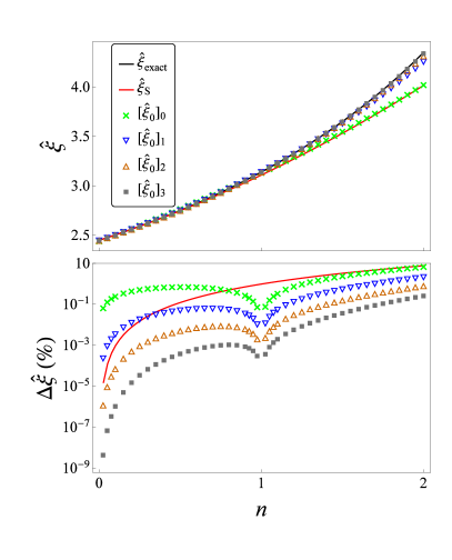
Figure 1: In the upper panel, the value of the normalised radius $\hat{\xi}$ is plotted as a function of the polytropic index $n$ for the numerically exact solution $\hat{\xi}_{\text{exact}}$ (black line), the SDEM approximants about $n=0$, $[\hat{\xi}_{0}]_{j}$ in equation (62) for $j=0$ (green cross), $j=1$ (blue triangle), $j=2$ (orange triangle) and $j=3$ (grey square), and the second order DEM approximation about $n=0$, $\hat{\xi}_{\text{S}}$ (see equation (19), red line). The associated error plot is shown in the lower panel, where $\Delta\hat{\xi}=|\hat{\xi}-\hat{\xi}_{\text{exact}}|/\hat{\xi}_{\text{exact}}\times 100\%$ represents the percentage error of the approximant.

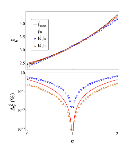
Figure 2: In the upper panel, the value of the normalised radius $\hat{\xi}$ is plotted as a function of the polytropic index $n$ for the numerically exact solution $\hat{\xi}_{\text{exact}}$ (black line), the SDEM approximants about $n=1$, $[\hat{\xi}_{1}]_{j}$ in equation (62) for $j=0$ (blue triangle) and $j=1$ (orange triangle), and the second order DEM approximation about $n=1$, $\hat{\xi}_{\text{B}}$ (see equation (23), red line). The associated error plot is shown in the lower panel, where $\Delta\hat{\xi}=|\hat{\xi}-\hat{\xi}_{\text{exact}}|/\hat{\xi}_{\text{exact}}\times 100\%$ represents the percentage error of the approximant.

In the upper panel of Figure 1, we have plotted the normalised radius $\hat{\xi}(x)$ against the polytropic index $n$. In particular, we compare the numerically exact value of the normalised radius, $\hat{\xi}_{\text{exact}}$, with the leading four perturbative approximations $[\hat{\xi}_{0}]_{j}$ ($j=0,1,2,3$) obtained from the SDEM about the incompressible limit $n=0$. As could be seen from the lower panel of Figure 1, where the percentage error $\Delta\hat{\xi}\equiv|\hat{\xi}-\hat{\xi}_{\text{exact}}|/\hat{\xi}_{\text{exact}}\times 100\%$ is shown as a function of $n$ for different approximants, the accuracy of the SDEM approximants $[\hat{\xi}_{0}]_{j}$ improves by two orders of magnitude over the interval $n\in[0,2]$ for each unit increment in the perturbation order $j$. It suggests that the proposed SDEM is able to offer rapid and uniform convergence. Moreover, the dips of the SDEM approximants at $n=0$ and $n=1$ in this error plot correspond to the fact that the SDEM approximants are exact at these two points. It is interesting to note that the SDEM approximant developed about $n=0$ is also exact at $n=1$. Such an unexpected result can be understood from equation (62), which guarantees that $[\hat{\xi}_{0}]_{j}$ is equal to $\pi$, which is the exact value at $n=1$, irrespective of the value of the scale factor $S$. In fact, this is the reason why we have chosen the normalisation factor in such a way that the first zero occurs at $z=\pi$ in the new length scale in equation (28). It is also worth noting that the second order SDEM approximant $[\hat{\xi}_{0}]_{2}$ is more accurate than its DEM counterpart $\hat{\xi}_{\text{S}}$ obtained by Seidov (2004) (see equation (19)) throughout the entire interval for $n$ in $[0,2]$. The underlying reason for the high accuracy achievable in the SDEM is the introduction of the scale factor $S(n)$, which leads to an effective resummation of the series obtained from the DEM.

Similarly, in Figure 2, we contrast $\hat{\xi}_{\text{exact}}$ with the leading two perturbative approximations $[\hat{\xi}_{1}]_{j}$ ($j=0,1$) obtained from the SDEM about $n=1$. As the approximants are exact at $n=1$, there are dips in the error plot (the lower panel of Figure 2) at $n=1$. Also, the first order SDEM approximant $[\hat{\xi}_{1}]_{1}$ outperforms the second order DEM counterpart $\hat{\xi}_{\text{B}}$ (see equation (23)) obtained by Bender et al. (1989) throughout the entire interval for $n$ in $[0,2]$. This once again confirms the power of the scale factor $S(n)$.

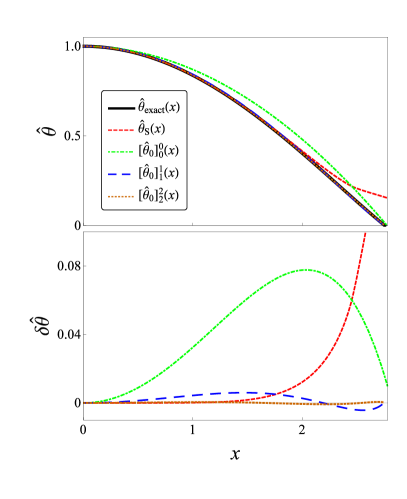
Figure 3: In the upper panel, for the case of $n=0.5$, we show the numerically exact polytrope function $\hat{\theta}_{\text{exact}}(x)$ (black line), the corresponding diagonal SDEM approximants $[\hat{\theta}_{0}]_{j}^{j}(x)$ about $n=0$ (see (63)) for $j=0$ (green dot-dashed), $j=1$ (blue long dashed) and $j=2$ (orange dotted), and the first order DEM result about $n=0$, $\hat{\theta}_{\text{S}}(x)$ (see equation (18), red dashed). As $\hat{\theta}_{\text{S}}(x)$ is ill-defined in real for $x>\sqrt{6}$, we take its real part in the plot. In the lower panel, the associated deviation from the numerically exact solution, $\delta\hat{\theta}(x)\equiv\hat{\theta}(x)-\hat{\theta}_{\text{exact}}(x)$ is shown under the same legend.

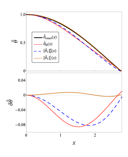
Figure 4: In the upper panel, for the case of $n=0.5$, we show the numerically exact polytrope function $\hat{\theta}_{\text{exact}}(x)$ (black line), the corresponding diagonal SDEM approximants $[\hat{\theta}_{0}]_{j}^{j}(x)$ about $n=1$ (see (63)) for $j=0$ (blue long dashed) and $j=1$ (orange dotted), and the first order DEM result about $n=1$, $\hat{\theta}_{\text{B}}(x)$ (see equation (20), red dashed). In the lower panel, the associated deviation from the numerically exact solution, $\delta\hat{\theta}(x)\equiv\hat{\theta}(x)-\hat{\theta}_{\text{exact}}(x)$ is shown under the same legend.

Next, in Figure 3 we study the accuracy of the normalised polytrope function $\hat{\theta}(x)$ obtained from the SDEM and the DEM approximants expanded about the incompressible limit where $n=0$ for a typical case of $n=0.5$. In the upper panel, the numerically exact polytrope function $\hat{\theta}_{\text{exact}}(x)$, the leading three diagonal SDEM approximants $[\hat{\theta}_{0}]_{j}^{j}(x)$ about $n=0$ (see equation (63)) for $j=0,1,2$, and the first order DEM result about $n=0$, $\hat{\theta}_{\text{S}}(x)$ (see equation (18)) are shown. Besides, in the lower panel the associated deviation from the numerically exact solution, $\delta\hat{\theta}(x)\equiv\hat{\theta}(x)-\hat{\theta}_{\text{exact}}(x)$ is also shown. We observe that the diagonal SDEM approximants $[\hat{\theta}_{0}]_{j}^{j}(x)$ in general carry bounded error within the entire polytrope. In particular, the accuracy improves order by order, and the deviation of the second order diagonal SDEM approximant $[\hat{\theta}_{0}]_{2}^{2}$ from the exact solution is less than 0.01 in the whole range. On the other hand, the approximant $\hat{\theta}_{\text{S}}(x)$ obtained from the DEM is also accurate for small $x$, but the accuracy declines rapidly when $x$ approaches $\sqrt{6}$. In fact, $\hat{\theta}_{\text{S}}(x)$ becomes complex-valued for $x$ greater than $\sqrt{6}$, the normalised radius of an incompressible polytrope, and as a consequence we have to take its real part in the plot.

We perform a similar analysis in Figure 4 by contrasting $\hat{\theta}_{\text{exact}}(x)$ with the diagonal SDEM and the DEM approximants expanded about $n=1$ for the case $n=0.5$. We see that the accuracies of the zeroth order diagonal SDEM approximant $[\hat{\theta}_{1}]_{0}^{0}$ and the first order DEM approximant $\hat{\theta}_{\text{B}}(x)$ (see equation (20)) are comparable. On the other hand, the first order diagonal SDEM approximant $[\hat{\theta}_{1}]_{1}^{1}$ carries a small error (less than 0.01) throughout the entire polytrope and is overall much better than $\hat{\theta}_{\text{B}}(x)$.

In contrast to the case studied in Figure 3, $\hat{\theta}_{\text{B}}(x)$ shown in Figure 4 is still well behaved near the surface of the polytrope. Such a qualitative difference can be understood as follows. In the case considered in Figure 4, the polytropic index is 0.5, which is less than the perturbation centre $n=1$. As mentioned above, $\hat{\xi}$ increase with increasing polytropic index. The radius of the polytrope (with $n=0.5$) considered in Figure 4 is thus less than that of the unperturbed one (with $n=1$). As a result, $\hat{\theta}_{\text{B}}(x)$ remains real in the entire polytrope. If, instead, a polytrope with a polytropic index greater than unity is considered, $\hat{\theta}_{\text{B}}(x)$ still becomes complex valued near the surface of the polytrope where $x$ is larger than $\pi$, the normalised radius of a polytrope with $n=1$, as in the case discussed in Figure 3.

It is worthwhile to note that the major distinction between our present work and the DEM calculations by Bender et al. (1989) and Seidov (2004) is the introduction of the simultaneous scale transformations shown in equations (27) and (28). Through such a scale transformation we have essentially performed a resummation of the original series obtained by the DEM, directly leading to the high accuracy of the SDEM. In fact, it can be shown that the results derived by the DEM can be recovered through (i) expanding the SDEM results in powers of $n-1$ (or $n$), respectively; and (ii) truncating the resulting series at suitable orders.

5 Mass of polytropes

Here we set to determine the local approximation of the mass of a polytrope, $M$, as a function of the polytropic index $n$ by SDEM analyses about $n=0$ or $n=1$. Furthermore, in Section 6, we will use these local approximations to determine a global approximate expression for $M$ that is valid and accurate throughout the entire interval $n\in[0,5]$.

The mass of a polytrope is given by:

$$M=\left[\frac{(n+1)K}{4\pi G}\right]^{3/2}\rho_{c}^{(3-n)/(2n)}m(n),$$ (64)

where the dimensionless mass function $m(n)$ and the second moment of $\Theta^{n}$, $\mu(n)$, are respectively defined by:

$$m(n)=\frac{4}{\pi^{2}}\hat{\xi}^{3}\mu(n),$$ (65)

$$\mu(n)=\int_{0}^{\pi}[\Theta(z)]^{n}z^{2}dz.$$ (66)

As both $\hat{\xi}$ and $\Theta(z)$ have been obtained perturbatively through the SDEM in the previous section, $m(n)$ can be found accordingly. Besides, it is interesting to note from equation (64) that the mass $M$ increases (decreases) with an increment in $\rho_{c}$ for $n<3$ ($n>3$). As the mass $M$ should be an increasing function of the central density $\rho_{c}$ for stable stars with a given equation of state, a polytropic star is thus stable (unstable) if the polytropic index is less (greater) than 3, which is in agreement with the standard result obtained from stability analysis (see, e.g., Shapiro & Teukolsky, 1983).

Using the SDEM results at $n=0$ or $1$, we form the local approximant of the dimensionless mass $m(n)$, which is denoted by $[m_{p}]^{k}_{j}(n)$ (with $p=0$ or $1$ signifying the perturbation centre):

$$[m_{p}]^{k}_{j}(n) =\frac{4}{\pi^{2}}\left\{[\hat{\xi}_{p}]_{j}(n)\right\}^{3}[\mu_{p}]_{k}(n),$$ (67)

where the approximant of the normalised radius, $[\hat{\xi}_{p}]_{j}(n)$, is defined in the previous section, and $[\mu_{p}]_{k}$ is similarly defined:

$$[\mu_{p}]_{k}(n) =\mu_{p}^{(0)}+\ldots+(n-p)^{k}\mu_{p}^{(k)},$$ (68)

and the subscript $j$ (superscript $k$) of the notation $[m_{p}]^{k}_{j}(n)$ denotes the perturbation order of the normalized radius $\hat{\xi}(n)$ ($\mu(n)$).

We first consider the case at $p=0$. We note here that in general $\mu_{0}^{(i)}$ is completely specified by $\Theta_{0}^{(0)},\Theta_{0}^{(1)},\ldots,\Theta_{0}^{(i-1)}$. Similarly, we expand the dimensionless density term $[\Theta(z)^{n}]$ in powers of $n$:

$$\Theta^{n}= 1+n\ln\Theta_{0}^{(0)}+n^{2}\left(\frac{1}{2}\ln^{2}\Theta_{0}^{(0)}+\frac{\Theta_{0}^{(1)}}{\Theta_{0}^{(0)}}\right)+n^{3}\bigg{(}\frac{1}{6}\ln^{3}\Theta_{0}^{(0)}$$

$$+\frac{\Theta_{0}^{(1)}\ln\Theta_{0}^{(0)}}{\Theta_{0}^{(0)}}-\frac{\Theta_{0}^{(1)}{}^{2}}{2\Theta_{0}^{(0)}{}^{2}}+\frac{\Theta_{0}^{(2)}}{\Theta_{0}^{(0)}}\bigg{)}+O[n^{4}].$$ (69)

By integrating order by order in $n$, it follows directly from the expressions of $\Theta_{0}^{(0)}$, $\Theta_{0}^{(1)}$ and $\Theta_{0}^{(2)}$ obtained in Section 4, we determine:

$$\mu_{0}^{(0)} =\frac{\pi^{3}}{3}\approx 10.3354255601,$$ (70)

$$\mu_{0}^{(1)} =\frac{\pi^{3}}{9}\left(-4+3\ln 2\right)\approx-13.2331926532,$$ (71)

$$\mu_{0}^{(2)} =\frac{\pi^{3}}{54}\left(-21\pi^{2}+200+12\ln 2+36\ln^{2}2\right)$$

$$\approx 10.5377600301,$$ (72)

$$\mu_{0}^{(3)} =\frac{\pi^{3}}{81}\bigg{(}-3464+75\pi^{2}-210\ln 2-63\pi^{2}\ln 2$$

$$\quad+180\ln^{2}2+36\ln^{3}2+2646\zeta(3)\bigg{)}$$

$$\approx-8.12140718515.$$ (73)

From the SDEM calculations at $n=0$, we observe that the approximant $[\mu_{0}]_{k}(n)$ appears to form a slowly converging alternating series with a small radius of convergence in $n$. To accelerate the convergence of the series, we apply the Padé resummation technique to rewrite the approximant $[\mu_{0}]_{k}(n)$ as a rational function, while respecting the series expansion of the original series. In our case, we employ a $[2,1]$ Padé approximant, $[\mu_{0}]_{[2,1]}(n)$, given explicitly by:

$$[\mu_{0}]_{[2,1]}(n)= \frac{1}{\left(\mu_{0}^{(2)}+n\mu_{0}^{(3)}\right)}\bigg{\{}\mu_{0}^{(0)}\mu_{0}^{(2)}+n\bigg{(}\mu_{0}^{(1)}\mu_{0}^{(2)}$$

$$-\mu_{0}^{(0)}\mu_{0}^{(3)}\bigg{)}+n^{2}\left[(\mu_{0}^{(2)})^{2}-\mu_{0}^{(1)}\mu_{0}^{(3)}\right]\bigg{\}},$$ (74)

to match $[\mu_{0}]_{3}(n)$ up to the third order (see, e.g., Baker & Graves-Morris, 1996, for the construction and the notation of Padé approximants), in the hope that the alternating behaviour is mimicked by the linear term in the denominator.

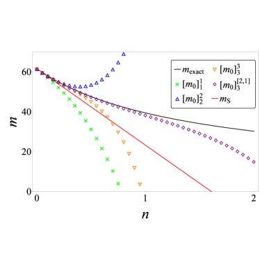
Figure 5: The value of the mass $m$ is plotted as a function of the polytropic index $n$ for the numerically exact solution (black line); the diagonal SDEM approximants about $n=0$, $[m_{0}]_{j}^{j}$ in equation (67) for $j=1$ (green cross), $j=2$ (blue triangle), and $j=3$ (orange triangle); the $[2,1]$ Padé approximant, $[m_{0}]^{[2,1]}_{3}(n)$ in equation (75) (purple rhombus); and the first order DEM result about $n=0$ (see equation (76), red line).

In Figure 5, we compare the accuracy of several local approximants of $m$ about $n=0$, including $[m_{0}]^{1}_{1}$, $[m_{0}]^{2}_{2}$, $[m_{0}]^{3}_{3}$, and the Padé approximant:

$$[m_{0}]^{[2,1]}_{3}(n)= \frac{4}{\pi^{2}}\left\{[\hat{\xi}_{0}]_{3}(n)\right\}^{3}[\mu_{0}]_{[2,1]}(n),$$ (75)

where the third order approximant of the normalized radius, $[\hat{\xi}_{0}]_{3}(n)$, is adopted specifically for illustration purpose. Numerical results reveal that, except for the Padé approximant $[m_{0}]^{[2,1]}_{3}(n)$, the other approximants are only accurate near the perturbation center $n=0$ and have a narrow interval of validity. The errors build up rapidly when $n$ is close to unity. In contrast, the $[2,1]$ Padé approximant $[m_{0}]^{[2,1]}_{3}(n)$ closely resembles the numerical solution over an extended interval from $n=0$ to $n\approx 1.5$. It confirms the necessity of an appropriate series resummation.

We also show in Figure 5 the approximant of the mass derived from the DEM (Seidov, 2004), which is given by:

$$m_{\text{S}}(n)=8\sqrt{6}\pi+\frac{4\sqrt{6}\pi}{3}(-37+48\ln 2)n+O[n^{2}].$$ (76)

The performance of $m_{\text{S}}(n)$ is quite close to that of other direct SDEM expansions such as $[m_{0}]^{1}_{1}$, $[m_{0}]^{2}_{2}$, $[m_{0}]^{3}_{3}$. It is accurate only within a narrow range extending from $n=0$ to $n\approx 0.5$. Once again it pinpoints the importance of the application of the Padé approximation in order to enlarge the domain of validity of the approximant of the mass.

Here we put forward an argument to support the necessity of introducing the Padé approximant to resum the expansion of $\mu(n)$. We notice that, to the leading order, the second moment integral $\mu(n)$ is given by:

$$\mu(n)=\int_{0}^{\pi}z^{2}(1-\frac{z^{2}}{\pi^{2}})^{n}dz=\frac{\pi^{7/2}\Gamma(n+1)}{4\Gamma(n+5/2)},\quad\mbox{for}\quad n>-1,$$ (77)

where $\Gamma(z)$ is the gamma function defined by (see, e.g., Olver et al., 2010):

$$\Gamma(z)=\int_{0}^{\infty}t^{z-1}e^{-t}dt.$$ (78)

It is a well-known fact that $\Gamma(n+1)$ is a meromorphic function with simple poles at $n=-1,-2,-3,\ldots$. In the SDEM calculations about $n=0$, we have expanded the $\Theta^{n}$ term into a power series of $n$, and the $n$-series expansion has the radius of convergence $1$ due to the nearest singularity at $n=-1$. It then readily explains the narrow interval of validity of the direct expansions of $\mu(n)$ about the point $n=0$. On the other hand, numerical investigation suggests that the integral for $\mu(n)$ (see equation (66)) can be computed more accurately if $[\Theta(z)]^{n}$ there is expanded through binomial expansion instead of the SDEM. However, the resultant integrals do not have simple solutions in terms of elementary mathematical functions.

On the other hand, we can similarly apply the SDEM to expand the integral $\mu(n)$ about $n=1$ to form a power series of $n-1$ (see equation (68)), with the leading two expansion coefficients given explicitly by:

$$\mu_{1}^{(0)} =\pi,$$ (79)

$$\mu_{1}^{(1)} =\frac{\pi}{4}[\text{Cin}(2\pi)+6-4\ln(2\pi)]-\frac{1}{2}\text{Si}(2\pi)$$

$$\approx-3.68507639562.$$ (80)

However, higher order coefficients are not shown due to their cumbersome expressions. Although we could still find accurate local approximant of $m(n)$ from $\mu_{1}^{(0)}$ and $\mu_{1}^{(1)}$, its applicability is limited within a narrow region where $n\approx 1$. Instead of further expanding $\mu(n)$ about $n=1$, we shall combine all the information resulting from expansion about $n=0$ and $n=1$ in Section 6 using the two-point Padé approximation technique to enhance the accuracy and extend the interval of validity of the relevant approximant.

6 Global Approximation of Polytropes

So far we have determined the variations of the polytrope function, the scale factor and the mass up to the third order about $n=0$, as well as such variations up to the first order about $n=1$ based on the SDEM. These results constitute local approximations about $n=0$ and $n=1$. On the other hand, in addition to the exact solution of the polytrope function at $n=5$ (see equation (10)), Buchdahl (1978) obtained the following leading order approximation of $\hat{\xi}(n)$:

$$\hat{\xi}(n)=\frac{32\sqrt{3}}{\pi(5-n)}+O[1],$$ (81)

which is valid for polytropes with $n$ less than and close to 5 (see Appendix A for a brief account of Buchdahl’s argument). In this section, starting from the perturbation results as well as the analytically exact solution about $n=0,1$ and $5$, we derive globally valid, approximate expressions for the normalised radius, the the mass and the polytrope function and as a function of the polytropic index $n$. The spirit is to construct expressions that respect the local variations about $n=0$ and $n=1$, and also match the exact value or the asymptotic behaviour about $n=5$. These global approximants will be compared to other existing approximants reviewed in Section 3 and Appendix A. For ease of reference, the useful results are presented in a self-contained manner in Appendix B.

6.1 Normalised radius

As the normalised radius of a polytrope is directly proportional to $S(n)^{(n-1)/2}$ (see equation (28)), we first look for a global approximant of the scale factor $S$. A modified $[3,2]$ Padé approximant of $S(n)$ is proposed:

$$S_{\text{g}}(n)=\frac{a_{1}+a_{2}n+a_{3}n^{2}+a_{4}n^{3}}{\sqrt{5-n}\big{(}1+a_{5}n+a_{6}n^{2}\big{)}},$$ (82)

where the constants $a_{1}$, …, $a_{6}$ are determined by the SDEM results of $S(n)$ about $n=0$ and $n=1$, and the square root term in the denominator is chosen to match the leading behaviour of the radius when $n$ approaches $5$ (see equation (81) and Appendix A).

Using the perturbation coefficients $S_{0}^{(0)}$, $S_{0}^{(1)}$, $S_{0}^{(2)}$, $S_{0}^{(3)}$, $S_{1}^{(0)}$ and $S_{1}^{(1)}$, whose values are given in equations (37), (39), (41), (48), (58) and (60), respectively, we can fix the values of $a_{1},\ldots,a_{6}$:

$$\begin{split}&a_{1}\approx 3.678184391977817,\\ &a_{2}\approx-0.12127837785202653,\\ &a_{3}\approx-0.0820898766826553,\\ &a_{4}\approx 0.0030327766768460046,\\ &a_{5}\approx 0.00858273787249898,\\ &a_{6}\approx-0.018845815183087977.\end{split}$$

Moreover, we have checked that the Padé approximant in equation (82) does not diverge within the physical range $n\in[0,5)$.

When $S_{\text{g}}(n)$ is substituted into equation (28), accurate values of the normalised radius can readily be reproduced. However, to further improve the accuracy, we propose the following semi-analytical approximant of the normalised radius:

$$\hat{\xi}_{\text{g}}(n)=\frac{\pi S_{\text{g}}(n)^{(n-1)/2}}{1+a_{0}n^{8}(n-1)^{8}}.$$ (83)

Here the constant $a_{0}$ is fixed by imposing the leading bahaviour at $n=5$ in equation (81), which shows that as $n\rightarrow 5$ from the left, $\hat{\xi}(n)\rightarrow(32\sqrt{3})/[\pi(5-n)]$. While the simple pole-like divergence is taken care of in the scale factor, the constant $a_{0}\approx 1.5996644405401317\times 10^{-17}$ now accounts for the residue-like factor $32\sqrt{3}/\pi$. Besides, the high power $n^{8}(n-1)^{8}$ is added to minimize the influence of the denominator on the local approximations around $n=0$ and $n=1$.

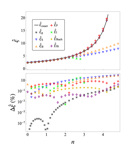
Figure 6: In the upper panel, the value of the normalised radius $\hat{\xi}$ is plotted as a function of the polytropic index $n$ for the numerically exact solution $\hat{\xi}_{\text{exact}}$ (black line), $\hat{\xi}_{\text{g}}$ in equation (83) (grey square), $\hat{\xi}_{\text{S}}$ in equation (19) (blue triangle), $\hat{\xi}_{\text{B}}$ in equation (23) (orange triangle), $\hat{\xi}_{\text{P}}$ (see Appendix A and equation (A), red plus), $\hat{\xi}_{\text{I}}$ in equation (92) (green cross), $\hat{\xi}_{\text{Buch}}$ in equation (94) (yellow star), and $\hat{\xi}_{\text{fit}}$ in equation (95) (purple rhombus). The associated percentage error plot in logarithmic scale is shown in the lower panel, with $\Delta\hat{\xi}=|\hat{\xi}-\hat{\xi}_{\text{exact}}|/\hat{\xi}_{\text{exact}}\times 100\%$.

We show the global approximant of the normalised radius, $\hat{\xi}_{\text{g}}(n)$ in equation (83), as a function of $n$ in Figure 6, where the exact numerical value of the normalised radius, $\hat{\xi}_{\text{exact}}(n)$, and other approximants reviewed in the text and Appendix A (including $\hat{\xi}_{\text{S}}(n)$, $\hat{\xi}_{\text{B}}(n)$, $\hat{\xi}_{\text{P}}(n)$ $\hat{\xi}_{\text{I}}(n)$, $\hat{\xi}_{\text{Buch}}(n)$ and $\hat{\xi}_{\text{fit}}(n)$) are shown as well. First of all, we see that the normalised radius increases with the polytropic index $n$. It agrees with our intuition that the density tail of a polytrope extends with increasing polytropic index $n$. Secondly, as for the accuracy of various approximation schemes (see the lower panel of Figure 6), we find that $\hat{\xi}_{\text{g}}(n)$ is better than other existing approximations. While the approximants derived from the DEM (Seidov, 2004; Bender et al., 1989), $\hat{\xi}_{\text{S}}(n)$ in equation (19) and $\hat{\xi}_{\text{B}}(n)$ in equation (23), are only accurate in the vicinity of their respective perturbation centers, the error of $\hat{\xi}_{\text{g}}(n)$ stays below $1$ per cent throughout the physical range $n\in[0,5)$. In fact, it is less than $8.1\times 10^{-7}$ per cent for $n\in[0,1]$. In comparison, over the same range $n\in[0,1]$, the maximum error of $\hat{\xi}_{\text{P}}(n)$ in equation (A) (Pascual, 1977), $\hat{\xi}_{\text{Buch}}(n)$ in equation (94) (Buchdahl, 1978) and $\hat{\xi}_{\text{fit}}(n)$ in equation (95) (Iacono & De Felice, 2015) reach $2.6$, $0.055$ and $0.079$ per cent, respectively. Besides, the Padé approximant $\hat{\xi}_{\text{I}}(n)$ in equation (92) (Iacono & De Felice, 2015) diverges at $n=3.050$, and is ill-defined in real beyond that point.

6.2 Mass

We construct an approximant that matches the SDEM results about $n=0$ and $n=1$, as well as the analytically exact value of the mass $m$ at $n=5$. It follows directly from (10) that:

$$m(n=5)=4\pi\int_{0}^{\infty}\frac{x^{2}}{(1+x^{2}/3)^{5/2}}dx=4\pi\sqrt{3}.$$ (84)

As shown in equation (82), $\hat{\xi}_{\rm g}$ diverges as $(5-n)^{-1}$ as $n$ approaches 5 from the left (see equations (82) and (83)). For $m$ to remain finite and non-vanishing at $n=5$, we hypothesize an approximant of the second moment integral $\mu_{\rm g}(n)$ to carry a factor of $(5-n)^{3}$ in the form:

$$\mu_{\rm g}(n)=(5-n)^{3}\frac{b_{1}+nb_{2}+n^{2}b_{3}+n^{3}b_{4}}{1+nb_{5}+n^{2}b_{6}},$$ (85)

where the real constants $b_{i}$ for $i=1,2,\ldots,6$ are to be determined by the SDEM results at $n=0$ (i.e., $\mu_{0}^{(0)}$, $\mu_{0}^{(1)}$, $\mu_{0}^{(2)}$, and $\mu_{0}^{(3)}$) and $n=1$ (i.e., $\mu_{1}^{(0)}$ and $\mu_{1}^{(1)}$). The values of these constants can be readily found from equations (70), (71), (72), (73), (79) and (80), which are given by:

$$\begin{split}&b_{1}\approx 0.08268340448079952,\\ &b_{2}\approx 0.0570923774427696,\\ &b_{3}\approx-0.0021371524111317,\\ &b_{4}\approx-0.000863277094516044,\\ &b_{5}\approx 1.370866096910041,\\ &b_{6}\approx 0.415498502167336.\end{split}$$

We check that the denominator vanishes at $n\approx-2.21$ and $n\approx-1.09$, so the Padé approximant does not diverge within the physical range $n\in[0,5]$. It echoes the leading behaviour of the mass in equation (77), that the $\Gamma(n+1)$ factor contains simple poles at $n=-1,-2,-3,\ldots$.

So far, we have imposed the SDEM results at $n=0$ and at $n=1$. To utilize the analytically exact value of $m(n=5)$, we propose an approximant in the form:

$$m_{\text{g}}(n)=4\pi S_{\text{g}}(n)^{3(n-1)/2}\mu_{\rm g}(n)+b_{0}(5-n)^{(15-3n)/4}n^{8}(n-1)^{8},$$ (86)

While the first term in the RHS of the above equation follows directly from equations (28) and (65), the second term is a correction term aimed at reproducing the exact mass at $n=5$ (see equation (84)). To this end, the real constant $b_{0}\approx-3.420867516502784\times 10^{-10}$ is chosen and the factor $(5-n)$ is raised to the power $(15-3n)/4$ so that the correction term matches the behaviour of $S_{\text{g}}^{3(n-1)/2}\mu_{\rm g}$ as $n$ approaches $5$ from the left. Besides, we have multiplied the correction term by a factor $n^{8}(n-1)^{8}$ to minimize the influence of the correction term on $m_{\text{g}}(n)$ for $n$ close to 0 or 1.

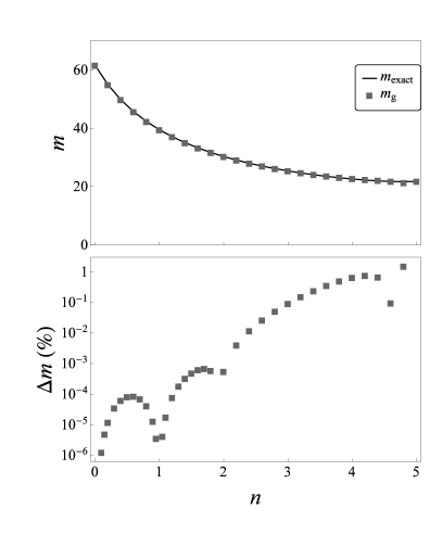
Figure 7: In the upper panel, the value of the dimensionless mass $m$ is plotted as a function of $n$ for the numerically exact solution (black line), and the global SDEM approximant $m_{\text{g}}$ in equation (86) (grey square), The associated error plot in logarithmic scale is shown in the lower panel, with $\Delta m=|m-m_{\text{exact}}|/m_{\text{exact}}\times 100\%$.

The numerical solution and the global approximant of the mass, $m_{\text{g}}(n)$, are plotted in Figure 7. We see that $m_{\text{g}}(n)$ can nicely approximate the numerical value with a maximum error of about $2\%$ in the whole range where $n\in[0,5]$. Such high degree of accuracy is achieved by incorporating the SDEM results obtained at $n=0$ and $n=1$ into a Padé approximant, together with a correction term such that $m_{\text{g}}(n)$ agrees with the analytically exact value at $n=5$. It is worthwhile to remark that such a global approximant of the mass is derived analytically from the SDEM without the help of any numerical fittings.

On the other hand, we can also see the dependence of the mass $m$ as a function of $n$ in Figure 7. While the polytropic tail lengthens with increasing polytropic index, the density decreases in the scaled frame $z$. Overall, the decrease of the density term dominates the lengthening of the polytropic tail, so that the total dimensionless mass decreases with increasing polytropic index $n$. Notice that the lengthening of the polytropic tail is less pronounced near the incompressible limit $n=0$, as could be seen in Figure 6. As a result, the mass decreases more rapidly near the incompressible limit $n=0$.

6.3 Normalised polytrope function

Based on the SDEM results at $n=0$ and $n=1$, we construct a two-point polynomial approximation for the polytrope function $\hat{\theta}_{\text{tp}}(x)$, by requiring its variations to match the local SDEM results about $n=0$ and $n=1$. The approximant is given by:

$$\hat{\theta}_{\text{tp}}(x)= \Theta_{0}^{(0)}(z_{\text{g}})+n\Theta_{0}^{(1)}(z_{\text{g}})+n^{2}\Theta_{0}^{(2)}(z_{\text{g}})+n^{3}\bigg{[}-4\Theta_{0}^{(0)}(z_{\text{g}})$$

$$-3\Theta_{0}^{(1)}(z_{\text{g}})-2\Theta_{0}^{(2)}(z_{\text{g}})+4\Theta_{1}^{(0)}(z_{\text{g}})-\Theta_{1}^{(1)}(z_{\text{g}})\bigg{]}$$

$$+n^{4}\bigg{[}3\Theta_{0}^{(0)}(z_{\text{g}})+2\Theta_{0}^{(1)}(z_{\text{g}})+\Theta_{0}^{(2)}(z_{\text{g}})$$

$$-3\Theta_{1}^{(0)}(z_{\text{g}})+\Theta_{1}^{(1)}(z_{\text{g}})\bigg{]},$$ (87)

where the scaled length scale $z_{\text{g}}=\pi x/\hat{\xi}_{\text{g}}(n)$.

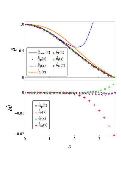
Figure 8: In the upper panel, for $n=1.5$, we plot the numerically exact polytrope function $\hat{\theta}_{\text{exact}}(x)$ (black solid line), the two-point SDEM approximant $\hat{\theta}_{\text{tp}}(x)$ in equation (6.3) (grey square), $\hat{\theta}_{\text{S}}(x)$ (Seidov, 2004) in equation (18) (blue dot-dashed), $\hat{\theta}_{\text{B}}(x)$ (Bender et al., 1989) in equation (20) (orange dotted), $\hat{\theta}_{\text{P}}(x)$ (Pascual, 1977) in equation (A) (red plus), $\hat{\theta}_{\text{I}}(x)$ (Iacono & De Felice, 2015) in equation (A) (green cross), and $\hat{\theta}_{\text{fit}}(x)$ (Iacono & De Felice, 2015) (see equation (95)) (purple rhombus) Plotted in the lower panel is the associated deviation from the exact polytrope function, $\delta\hat{\theta}=\hat{\theta}-\hat{\theta}_{\text{exact}}$ for the approximants, $\hat{\theta}_{\text{g}}(x)$, $\hat{\theta}_{\text{P}}(x)$, $\hat{\theta}_{\text{I}}(x)$, and $\hat{\theta}_{\text{fit}}(x)$.

Next, in the upper panel of Figure 8 we compare the two-point SDEM approximant of the polytrope function, $\hat{\theta}_{\text{tp}}(x)$ in equation (6.3), against other existing approximations, including the two formulae obtained from the DEM, i.e., $\hat{\theta}_{\text{S}}(x)$ in equation (18) (Seidov, 2004) and $\hat{\theta}_{\text{B}}(x)$ in equation (20) (Bender et al., 1989), and the two Padé approximants $\hat{\theta}_{\text{P}}(x)$ (see (A) and Pascual, 1977), $\hat{\theta}_{\text{I}}(x)$ and $\hat{\theta}_{\text{fit}}(x)$ (see (A) and Iacono & De Felice, 2015), for the case $n=1.5$. Several remarks about the performance of various approximants are in order. First, we note that $\hat{\theta}_{\text{tp}}(x)$ is indeed very close to the exact value $\hat{\theta}_{\text{exact}}(x)$ and their difference is smaller than 0.001 throughout the polytrope. Secondly, as mentioned previously, $\hat{\theta}_{\text{S}}(x)$ and $\hat{\theta}_{\text{B}}(x)$ are ill-defined in real for $x>\sqrt{6}$ and $x>\pi$, respectively, because they fail to capture the movement of the branch point singularity at the surface of the polytrope. We take the real part of $\hat{\theta}_{\text{S}}(x)$ and $\hat{\theta}_{\text{B}}(x)$ in this figure. Still, $\hat{\theta}_{\text{S}}(x)$ deviates significantly from the exact value near the surface of the polytrope. On the other hand, while $\hat{\theta}_{\text{B}}(x)$ can nicely approximate $\hat{\theta}_{\text{exact}}(x)$ at the centre and the surface of the polytrope, its accuracy worsens in the intermediate range.

As for case of the two analytically derived Padé approximants $\hat{\theta}_{\text{P}}(x)$ and $\hat{\theta}_{\text{I}}(x)$, which are obtained by resumming the series solution of the LEE about $x=0$, we see that they are highly accurate near $x=0$ but the error builds up all the way to the surface of the polytrope. In comparison, the two-point SDEM approximant $\hat{\theta}_{\text{tp}}(x)$ oscillates about the exact value with a tiny amplitude and is uniformly accurate throughout the entire physical region. The accuracy of the two-point SDEM approximant $\hat{\theta}_{\text{tp}}(x)$ is similar to that of the approximant $\hat{\theta}_{\text{fit}}(x)$, which are the only two approximations that are uniform throughout the physical domain of interest. A good approximation of the polytrope function near the surface is associated with an accurate determination of the radius. In the two-point SDEM analysis, the radius is accurately and analytically determined via a scale transformation, and could be systematically improved by increasing the perturbation order. The latter relies on least square fitting against numerical results, and its accuracy could be boosted by using more free parameters in the fitting.

As the normalised radius of the polytrope at $n=5$ is infinite, SDEM is not directly applicable at $n=5$. On other other hand, $\hat{\theta}_{\text{P}}(x)$ in equation (A) utilises the exact solution at $n=5$ by an ingenious variable transformation. For an analytical approximant that is accurate for all finite polytropes over the range of $n$ in $[0,5)$, we define an piecewise approximant to be

$$\hat{\theta}_{\text{g}}(x)=\begin{cases}\hat{\theta}_{\text{tp}}(x),&\text{for}\qquad 0\leq n\leq 2,\\ \hat{\theta}_{\text{P}}(x),&\text{for}\qquad 2<n<5.\end{cases}$$ (88)

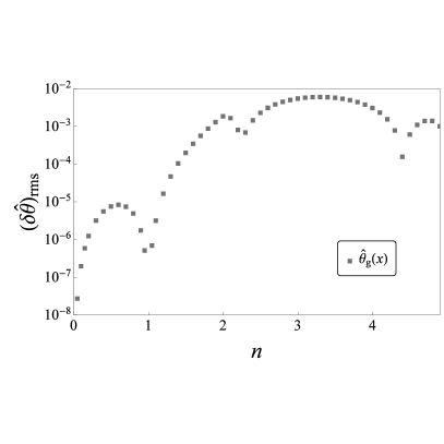
Figure 9: The root mean square error $(\delta\hat{\theta})_{\text{rms}}\equiv[\int_{0}^{\hat{\xi}}[\hat{\theta}(x)-\hat{\theta}_{\text{exact}}(x)]^{2}dx/\hat{\xi}]^{1/2}$ of the global approximant $\hat{\theta}_{\text{g}}(x)$ in equation (100) (grey square) is plotted against the polytropic index $n$.

In Figure 9, we see that the root mean square error $(\delta\hat{\theta})_{\text{rms}}\equiv[\int_{0}^{\hat{\xi}}[\hat{\theta}(x)-\hat{\theta}_{\text{exact}}(x)]^{2}dx/\hat{\xi}]^{1/2}$ of the approximant $\hat{\theta}_{\text{g}}(x)$ is less than $6.1\times 10^{-3}$ throughout the physical range of finite polytropes for $n\in[0,5)$. In particular, $(\delta\hat{\theta})_{\text{rms}}$ is within $8.4\times 10^{-6}$ between the two SDEM perturbation centres at $n=0$ and $1$. The error increases sharply from $n=1$ to $n=2$ signifying a decline of accuracy of the two-point SDEM approximant $\hat{\theta}_{\text{tp}}(x)$. Beyond $n=2$, the Padé approximant $\hat{\theta}_{\text{P}}(x)$ is more accurate than the two-point SDEM approximant $\hat{\theta}_{\text{tp}}(x)$. The Padé approximant $\hat{\theta}_{\text{P}}(x)$ is therefore used to define the global approximant of the normalised polytrope function.

7 Discussion and Conclusion

Motivated by the successful application of the DEM to the solution of the LEE (Bender et al., 1989; Seidov, 2004), we propose in the present paper the SDEM, an extension of the DEM, to remedy the inadequacy of the original scheme. The major problem with the LEE is the $\theta^{n}$ term, which in general ceases to be an analytic function at points where $\theta$ vanishes. In fact, the $\theta^{n}$ term could become complex-valued if $\theta$ is less than zero. As a consequence, the DEM is expected to break down outside the unperturbed polytrope (with $n=0$ or $1$). As the normalised radius of a polytrope is an increasing function of the polytropic index $n$, in the DEM the polytrope function of a perturbed polytrope with $n>0$ (or $n>1$) usually becomes complex near its surface. Even if the real part of such a complex function is taken, the accuracy of the resultant polytrope function could be poor (see Figures 3 and 8).

The SDEM is aimed at solving the above-mentioned problem. We exploit the scale invariance symmetry of the LEE to define an $n$-dependent scale transformation under which the scaled polytrope function $\Theta(z)$ is required to attain its first zero at the scaled coordinate $z=[S(n)]^{(1-n)/2}x=\pi$ regardless of the value of $n$. As a result, the domain of definition of the scaled LEE, where the polytrope function is real and non-negative, remains fixed throughout the perturbation scheme. In addition, the LEE is transformed from an initial value problem to an eigenvalue problem with the scale factor $S(n)$ being the eigenvalue (see equation (26)). In the present paper we have derived the perturbation corrections about $n=0$ up to the third order, and that about $n=1$ up to the first order. The local SDEM approximants are compared to the DEM results, and the former are found to be more accurate. In particular, the SDEM result is accurate within the entire polytrope and consequently the radius of a polytrope can also be determined accurately.

From the SDEM, we have derived the local as well as the global approximations to the normalised radius, the mass, and the normalised polytrope function as a function of the polytropic index $n$. The global approximant of the normalised radius, $\hat{\xi}_{\text{g}}(n)$ in equation (83), has a maximum percentage error of $8.1\times 10^{-7}$ per cent ($1$ per cent) for $n\in[0,1]$ ($n\in[0,5)$). Furthermore, the global SDEM approximant of the mass carries the maximum percentage error of $8.5\times 10^{-5}$ per cent ($2$ per cent) for $n$ in $[0,1]$ ($n\in[0,5)$). All such approximants are derived analytically without adoption of numerical fitting.

Two remarks about the scale transformation are in order. First, the choice of $\pi$ as the radius in the new scale indeed offers an additional benefit of an exact value of $\hat{\xi}(n=1)=\pi$ (see equation (28)) irrespective of the value of the scale factor $S(n)$. Therefore, as far as $\hat{\xi}$ is concerned, the SDEM expansion about $n=0$ is still able to yield the exact value at $n=1$ (see Figure 1). Secondly, the length dependence and the density dependence are separated in the SDEM calculations. For each physical quantity of a polytrope, each physical length factor is associated with a $S^{(n-1)/2}$ factor, or equivalently a $\hat{\xi}$ factor, while each density term is proportional to $\Theta(z)^{n}$.

In principle we can extend the SDEM calculations about $n=0$ and $n=1$ to high orders. The convergence property of such perturbation series is an interesting issue. On the other hand, it is also possible to apply the SDEM at other values of $n$ with no known closed form solution by numerical means. These researches are under way and relevant results will be reported elsewhere in due course.

Appendix A Other analytical approximations to the LEE

While the application of the DEM to the standard LEE has been reviewed in Section 3, here we summarize the results of some other relevant approximation schemes which have been used as the benchmarks for the accuracy of the SDEM established in the present paper.

In order to obtain a uniform approximation of the polytrope function and its normalised radius, based on the power series solution of the standard LEE and also in the light of the analytical solution of LEE at $n=5$, Pascual (1977) introduced a scaled coordinate $z_{\text{P}}$:

$$z_{\text{P}}=6\bigg{[}\bigg{(}1+\frac{x^{2}}{3}\bigg{)}^{1/2}-1\bigg{]}$$ (89)

to replace the standard independent variable $x$ of the LEE. After expressing the traditional power series solution of the LEE in a power series in $z_{\text{P}}$ and and performing a Padé resummation of such a series, Pascual (1977) obtained the Padé approximants of various orders for the polytrope function. In particular, the [2,2] Padé approximant (see, e.g., Baker & Graves-Morris, 1996) of the polytrope function is given by:

$$\hat{\theta}_{\text{P}}(x)= \bigg{[}45360(35+17n)+420\left(-630-367n+178n^{2}\right)z_{\text{P}}$$

$$+3(n-5)\left(1470-1393n+430n^{2}\right)z_{\text{P}}{}^{2}\bigg{]}\bigg{/}$$

$$\bigg{[}45360(35+17n)+420n(-61+178n)z_{\text{P}}$$

$$+5n\left(3703-919n+258n^{2}\right)z_{\text{P}}{}^{2}\bigg{]}.$$ (90)

We note that in Pascual’s original work, there is a typo in the numerator in the expression of $\hat{\theta}_{\text{P}}$. The number $-376n$ should be $-367n$ instead, and the correct expression is reproduced here. The normalised radius $\hat{\xi}_{\text{P}}$ of the standard LEE as a function of $n$ could be obtained by searching for the first zero of the numerator of $\hat{\theta}_{\text{P}}(x)$ and inverting the corresponding value of $x$, i.e., $\hat{\xi}_{\text{P}}$, from equation (89).

On the other hand, Iacono & De Felice (2015) expressed the the normalised polytrope function as a $[1,3]$ Padé approximant (see, e.g., Baker & Graves-Morris, 1996) in $x^{2}$ using the first five terms of the series solution of the LEE:

$$\hat{\theta}_{\text{I}}(x)= \bigg{(}1-\frac{x^{2}}{\hat{\xi}_{\text{I}}^{2}}\bigg{)}\bigg{/}\bigg{\{}1+x^{2}\left(\frac{1}{6}-\frac{1}{\hat{\xi}_{\text{I}}^{2}}\right)+\frac{x^{4}}{6}\left(\frac{1}{6}-\frac{n}{20}-\frac{1}{\hat{\xi}_{\text{I}}^{2}}\right)$$

$$+x^{6}\left[\frac{8n^{2}-47n+70}{15120}-\frac{10-3n}{60\hat{\xi}_{\text{I}}^{2}}\right]\bigg{\}},$$ (91)

where

$$\hat{\xi}_{\text{I}}(n)=\sqrt{\frac{6\left(12600-8460n+1440n^{2}\right)}{12600-13490n+4929n^{2}-610n^{3}}}.$$ (92)

As a result, the normalised radius of $\hat{\theta}_{\text{I}}(x)$ is simply equal to $\hat{\xi}_{\text{I}}(n)$, which is expressed as the square-root of a rational function of $n$ (see equation (92)). It could be easily determined that the denominator in equation (92) vanishes at $n\approx 3.05049$, signifying the failure of the approximant near and beyond $n\approx 3.05049$. The approximant is surprisingly accurate at $n=2$ with the approximate normalised radius $\hat{\xi}_{\text{I}}(n=2)=\sqrt{360/19}\approx 4.352857$ remarkably close to the numerical value $\hat{\xi}_{\text{exact}}\approx 4.352875$.

Other approximate expressions of $\hat{\xi}$ similar to that in equation (92) have also been found. Buchdahl (1978) found that the normalised radius $\hat{\xi}$ diverges like a simple pole from the left of $n=5$. The idea is to equate two expressions of the potential energy of polytropes, one involving the normalised polytrope function $\hat{\theta}$ and another involving macroscopic quantities the physical mass $M$, the physical radius $R$, and polytropic index $n$ only. Denote the potential energy by $U$, Buchdahl (1978) showed that:

$$U=-\frac{3GM^{2}}{(5-n)R}=\frac{GM^{2}}{a(\hat{\xi}^{2}\hat{\theta}^{\prime}(\hat{\xi}))^{2}}\int_{0}^{\hat{\xi}}x^{3}\hat{\theta}(x)\hat{\theta}^{\prime}(x)dx.$$ (93)

Substituting the analytical solution of the polytrope function at $n=5$ into equation (93), Buchdahl (1978) arrived at equation (81). By further interpolating with the analytically exact values of $\hat{\xi}$ at $n=0$ and $n=1$, Buchdahl (1978) proposed a [1,2] Padé approximant (see, e.g., Baker & Graves-Morris, 1996) in $n$ for $\hat{\xi}$:

$$\hat{\xi}_{\text{Buch}}(n)=\frac{12.2474487139(1-0.127597320123n)}{(5-n)(1-0.149738026390n)},$$ (94)

This simple formula is more accurate than the approximations derived from the series solution of the LEE for values of $n>2$, because it does not explicitly depend on the variation of the polytrope function with the polytropic index $n$, while the series solution converges slowly near the surface, and even diverges in the interior of the polytrope for $n>1.9121$ (Hunter, 2001).

Following Buchdahl (1978), Iacono & De Felice (2015) proposed a [2,2] Padé approximant (see, e.g., Baker & Graves-Morris, 1996) in $n$ for $\hat{\xi}$:

$$\hat{\xi}_{\text{fit}}(n)=\frac{12.2378-1.2249n+0.0187n^{2}}{(5-n)(1-0.1223n)}.$$ (95)

However, except for the factor $(5-n)$, the coefficients in the above expression have been determined with nonlinear least-square fitting to numerical data resulting from Runge-Kutta integrations for the range where $0\leq n<5$. Overall, the least-square fitted approximant is more accurate than that by Buchdahl (1978) for the extra free parameter in the numerator, except near the points $n=0$, $1$ and $5$ where the LEE admits a closed form solution for the analytical interpolation. Iacono & De Felice (2015) proposed to replace $\hat{\xi}_{\text{I}}$ by $\hat{\xi}_{\text{fit}}$ in equation (A) to yield an approximation, which is more accurate near the surface, at a slight compensation of accuracy near the origin, and we denote such an approximation by $\hat{\theta}_{\text{fit}}$.

Appendix B List of Useful Formulae

For ease of reference, in the following we quote the global approximate expressions of the normalised radius $\hat{\xi}$, the mass $m$, and the normalised polytrope function $\hat{\theta}(x)$.

B.1 Radius and normalised radius

For a polytrope of central density $\rho_{c}$ under the polytropic equation of state $P(r)=K[\rho(r)]^{1+1/n}$, its radius is equal to:

$$R=\sqrt{\frac{K(n+1)}{4\pi G}}\rho_{c}^{(1-n)/(2n)}\hat{\xi}(n)=a\hat{\xi}(n),\\$$ (96)

where $\hat{\xi}$ is the first zero of the the normalised polytrope function, approximately given by the global approximant:

$$\hat{\xi}_{\text{g}}(n)=\frac{\pi}{1+a_{0}n^{8}(n-1)^{8}}\bigg{[}\frac{a_{1}+a_{2}n+a_{3}n^{2}+a_{4}n^{3}}{\sqrt{5-n}\big{(}1+a_{5}n+a_{6}n^{2}\big{)}}\bigg{]}^{(n-1)/2},$$ (97)

with the constants $a_{i}$ for $i=0,1,2,\ldots,6$ determined by the proposed SDEM as follows:

$$\begin{split}&a_{0}\approx 1.5996644405401317\times 10^{-17},\\ &a_{1}\approx 3.678184391977817,\\ &a_{2}\approx-0.12127837785202653,\\ &a_{3}\approx-0.0820898766826553,\\ &a_{4}\approx 0.0030327766768460046,\\ &a_{5}\approx 0.00858273787249898,\\ &a_{6}\approx-0.018845815183087977.\end{split}$$

The error of $\hat{\xi}_{\text{g}}(n)$ is within $8.1\times 10^{-7}$ per cent near the incompressible limit for $n$ in $[0,1]$, and $1$ per cent throughout the physical range of finite polytropes where $n$ is in $[0,5)$. The details could be could in Figure 6.

B.2 Mass

The physical mass $M$ of the same polytrope is given by:

$$M=\int_{0}^{R}\rho(r)4\pi r^{2}dr=M=\left[\frac{(n+1)K}{4\pi G}\right]^{3/2}\rho_{c}^{(3-n)/(2n)}m(n),$$ (98)

where $m$ is the dimensionless mass approximately equal to $m_{\text{g}}(n)$:

$$m_{\text{g}}(n)= b_{0}(5-n)^{(15-3n)/4}n^{8}(n-1)^{8}$$

$$+4\pi\bigg{[}\frac{a_{1}+a_{2}n+a_{3}n^{2}+a_{4}n^{3}}{\sqrt{5-n}\big{(}1+a_{5}n+a_{6}n^{2}\big{)}}\bigg{]}^{3(n-1)/2}$$

$$\times(5-n)^{3}\frac{b_{1}+nb_{2}+n^{2}b_{3}+n^{3}b_{4}}{1+nb_{5}+n^{2}b_{6}},$$ (99)

where the constants $a_{i}$ for $i=0,1,2,...,6$ are given above and the constants $b_{i}$ for $i=0,1,2,...,6$ are determined by the proposed SDEM:

$$\begin{split}&b_{0}\approx-3.420867516502784\times 10^{-10},\\ &b_{1}\approx 0.08268340448079952,\\ &b_{2}\approx 0.0570923774427696,\\ &b_{3}\approx-0.0021371524111317,\\ &b_{4}\approx-0.000863277094516044,\\ &b_{5}\approx 1.370866096910041,\\ &b_{6}\approx 0.415498502167336.\end{split}$$

The error is within $8.5\times 10^{-5}$ per cent for $n$ in $[0,1]$, and $2$ per cent throughout the physical range of finite polytropes where $n$ is in $[0,5)$. The details could be could in Figure 7.

B.3 Density and normalised polytrope function

For a polytrope of central density $\rho_{c}$, the normalised polytrope function $\hat{\theta}(x)$ is related to the density profile of the polytrope $\rho(r)=\rho_{c}[\hat{\theta}(r/a)]^{n}$. Using the scaled variables $z_{\text{g}}=(\pi r)/(a\hat{\xi}_{\text{g}})$ and $z_{\text{P}}=6[(1+x^{2}/3)^{1/2}-1]$, the normalised polytrope function is approximated piecewise using $\hat{\theta}(x)\approx\hat{\theta}_{\text{g}}(x)$, where:

$$\hat{\theta}_{\text{g}}(x)=\begin{cases}\hat{\theta}_{\text{tp}}(x),&\text{for}\qquad 0\leq n\leq 2,\\ \hat{\theta}_{\text{P}}(x),&\text{for}\qquad 2<n<5,\end{cases}$$ (100)

with the functions $\hat{\theta}_{\text{P}}(x)$ and $\hat{\theta}_{\text{tp}}(x)$ given by:

$$\hat{\theta}_{\text{P}}(x)= \bigg{[}45360(35+17n)+420\left(-630-367n+178n^{2}\right)z_{\text{P}}$$

$$+3(n-5)\left(1470-1393n+430n^{2}\right)z_{\text{P}}{}^{2}\bigg{]}\bigg{/}$$

$$\bigg{[}45360(35+17n)+420n(-61+178n)z_{\text{P}}$$

$$+5n\left(3703-919n+258n^{2}\right)z_{\text{P}}{}^{2}\bigg{]},$$ (101)

$$\begin{split}\hat{\theta}_{\text{tp}}(x)=&\Theta_{0}^{(0)}(z_{\text{g}})+n\Theta_{0}^{(1)}(z_{\text{g}})+n^{2}\Theta_{0}^{(2)}(z_{\text{g}})+n^{3}\bigg{[}-4\Theta_{0}^{(0)}(z_{\text{g}})\\ &-3\Theta_{0}^{(1)}(z_{\text{g}})-2\Theta_{0}^{(2)}(z_{\text{g}})+4\Theta_{1}^{(0)}(z_{\text{g}})-\Theta_{1}^{(1)}(z_{\text{g}})\bigg{]}\\ &+n^{4}\bigg{[}3\Theta_{0}^{(0)}(z_{\text{g}})+2\Theta_{0}^{(1)}(z_{\text{g}})+\Theta_{0}^{(2)}(z_{\text{g}})\\ &-3\Theta_{1}^{(0)}(z_{\text{g}})+\Theta_{1}^{(1)}(z_{\text{g}})\bigg{]}.\end{split}$$ (102)

In the above the $\Theta$ functions are obtained perturbatively from the SDEM:

$$\Theta_{0}^{(0)}(z)=1-\frac{z^{2}}{\pi^{2}},$$ (103)

$$\Theta_{0}^{(1)}(z)= -4+\frac{4z^{2}}{\pi^{2}}\left(1-\ln 2\right)+\left(3-\frac{2\pi}{z}-\frac{z^{2}}{\pi^{2}}\right)\ln\left(1-\frac{z}{\pi}\right)$$

$$+\left(3+\frac{2\pi}{z}-\frac{z^{2}}{\pi^{2}}\right)\ln\left(1+\frac{z}{\pi}\right),$$ (104)

$$\Theta_{0}^{(2)}(z)= 40+\frac{7\pi^{2}}{3}+8\ln 2-14\ln^{2}2$$

$$+\left[\frac{7\pi^{2}}{3}-40+32\ln 2-8\ln^{2}2\right]\frac{z^{2}}{\pi^{2}}$$

$$+\left[-23+\frac{20\pi}{z}+\frac{3z^{2}}{\pi^{2}}+\big{(}14-\frac{10\pi}{z}-\frac{4z^{2}}{\pi^{2}}\big{)}\ln 2\right]$$

$$\quad\times\ln\left(1-\frac{z}{\pi}\right)+\left(\frac{3}{2}-\frac{\pi}{z}-\frac{z^{2}}{2\pi^{2}}\right)\ln^{2}\left(1-\frac{z}{\pi}\right)$$

$$+\left[-23-\frac{20\pi}{z}+\frac{3z^{2}}{\pi^{2}}+\big{(}14+\frac{10\pi}{z}-\frac{4z^{2}}{\pi^{2}}\big{)}\ln 2\right]$$

$$\quad\times\ln\left(1+\frac{z}{\pi}\right)+\left(\frac{3}{2}+\frac{\pi}{z}-\frac{z^{2}}{2\pi^{2}}\right)\ln^{2}\left(1+\frac{z}{\pi}\right)$$

$$+\left(1-\frac{z^{2}}{\pi^{2}}\right)\ln\left(1-\frac{z}{\pi}\right)\ln\left(1+\frac{z}{\pi}\right)$$

$$+\left(\frac{14\pi}{z}-14\right)\text{Li}_{2}\left(\frac{\pi-z}{2\pi}\right)$$

$$+\left(-\frac{14\pi}{z}-14\right)\text{Li}_{2}\left(\frac{\pi+z}{2\pi}\right),$$ (105)

$$\Theta_{1}^{(0)}(z)=\frac{\sin z}{z},$$ (106)

$$\Theta_{1}^{(1)}(z) =\frac{\sin z}{z}\bigg{[}1-\frac{\ln(2\pi)}{2}-\frac{\text{Si}(2\pi)}{4\pi}-\frac{\text{Cin}(2z)}{4}$$

$$+\frac{\ln z}{2}-\frac{1}{2}\ln(\sin z)\bigg{]}+\frac{\cos z}{z}\bigg{[}\frac{1}{2}z\ln(2\pi)$$

$$-\frac{1}{2}z\ln z+\frac{z\text{Si}(2\pi)}{4\pi}-\frac{\text{Si}(2z)}{4}+\frac{1}{2}\int_{0}^{z}\ln\sin tdt\bigg{]}.$$ (107)

The root mean square error of the approximant $\hat{\theta}_{\text{g}}(x)$ is within $8.4\times 10^{-6}$ for $n$ in $[0,1]$, and $6.1\times 10^{-3}$ for $n$ in $[0,5)$. For better illustrations, readers may refer to Figures 8 and 9.

References

- Baker & Graves-Morris (1996) Baker G., Graves-Morris P., 1996, Padé Approximants. Encyclopedia of Math. and Its Appl., Cambridge Univ. Press, NY
- Bender & Orszag (1978) Bender C., Orszag S., 1978, Advanced Mathematical Methods for Scientists and Engineers. McGraw-Hill, Inc.
- Bender et al. (1989) Bender C. M., Milton K. A., Pinsky S. S., Simmons Jr. L. M., 1989, J. Math. Phys., 30, 1447
- Binney & Tremaine (2011) Binney J., Tremaine S., 2011, Galactic Dynamics. Princeton Univ. Press, Princeton, NJ
- Buchdahl (1978) Buchdahl H. A., 1978, Aust J. Phys., 31, 115
- Chandrasekhar (1958) Chandrasekhar S., 1958, An introduction to the study of stellar structure. Dover Books on Astro. Series Vol. 2, Courier Corporation
- Chatziioannou et al. (2014) Chatziioannou K., Yagi K., Yunes N., 2014, Phys. Rev. D, 90, 064030
- Cox (1980) Cox J. P., 1980, Theory of Stellar Pulsation. Princeton Series in Astrophys., Princeton Univ. Press, Princeton, NJ
- Horedt (2004) Horedt G. P., ed. 2004, Polytropes - Applications in Astrophysics and Related Fields Astrophysics and Space Science Library Vol. 306. Springer, Netherlands
- Hunter (2001) Hunter C., 2001, MNRAS, 328, 839
- Iacono & De Felice (2015) Iacono R., De Felice M., 2015, Phys. Lett. A, 379, 1802
- Lewin (1991) Lewin L., 1991, Structural Properties of Polylogarithms. Math. Surveys and Monographs Vol. 37, Am. Math. Soc., Providence, RI
- Liu (1996) Liu F. K., 1996, MNRAS, 281, 1197
- Marinca & Herisanu (2012) Marinca V., Herisanu N., 2012, Nonlinear Dynamical Systems in Engineering: Some Approximate Approaches. Springer Berlin Heidelberg
- Nayfeh & Mook (1995) Nayfeh A., Mook D., 1995, Nonlinear Oscillations. Wiley, Weinheiin
- Olver et al. (2010) Olver F. W., Lozier D. W., Boisvert R. F., Clark C. W., 2010, NIST Handbook of Mathematical Functions, 1st edn. Cambridge Univ. Press, NY
- Pascual (1977) Pascual P., 1977, A&A, 60, 161
- Ramos (2008) Ramos J., 2008, Chaos, Solitons & Fractals, 38, 400
- Roxburgh & Stockman (1999) Roxburgh I. W., Stockman L. M., 1999, MNRAS, 303, 466
- Seidov (2004) Seidov Z. F., 2004, preprint, arXiv:astro-ph:0401359v1
- Seidov & Kuzakhmedov (1977) Seidov Z. F., Kuzakhmedov R. K., 1977, Soviet Ast., 21, 399
- Shapiro & Teukolsky (1983) Shapiro S. L., Teukolsky S. A., 1983, Black Holes, White Dwarfs, and Neutron Stars: The Physics of Compact Objects. Wiley, NY
- Sharaf & Alaqal (2012) Sharaf M. A., Alaqal M. A., 2012, Global J. of Sci. Frontier Res., 12, 31