Preconditioning PDE-constrained optimization with $\rm L^{1}$-sparsity and control constraints

Abstract

PDE-constrained optimization aims at finding optimal setups for partial differential equations so that relevant quantities are minimized. Including sparsity promoting terms in the formulation of such problems results in more practically relevant computed controls but adds more challenges to the numerical solution of these problems. The needed $\rm L^{1}$-terms as well as additional inclusion of box control constraints require the use of semismooth Newton methods. We propose robust preconditioners for different formulations of the Newton’s equation. With the inclusion of a line-search strategy and an inexact approach for the solution of the linear systems, the resulting semismooth Newton’s method is feasible for practical problems. Our results are underpinned by a theoretical analysis of the preconditioned matrix. Numerical experiments illustrate the robustness of the proposed scheme.

1 Introduction

Optimization is a crucial tool across the sciences, engineering, and life sciences and is thus requiring robust mathematical tools in terms of software and algorithms [23]. Additionally, over the last decade the need for sparse solutions has become apparent and the field of compressed sensing [8, 7] is a success story where mathematical tools have conquered all fields from image processing [22] to neuroscience [11].

One of the typical areas where optimization and sparsity promoting formulations are key ingredients is the optimization of functions subject to partial differential equation (PDE) constraints. In this field one seeks an optimal control such that the state of the system satisfies certain criteria, e.g. being close to a desired or observed quantity, while the control and state are connected via the underlying physics of the problem. This so-called state equation is typically a PDE of a certain type. While this is not a new problem [19, 37] the penalization of the control cost via an $\rm L^{1}$-norm requires different methodology from the classical $\rm L^{2}$-control term. Nonsmooth Newton methods [19, 17, 18, 38] have become the state-of-the-art when dealing with nonsmooth terms in PDE-constrained optimization problems as they still exhibit local superlinear convergence. In the case of a sparsity promoting $\rm L^{1}$-term within PDE-constrained optimization Stadler [34] considered the applicability and convergence of the nonsmooth Newton’s method. Herzog and co-authors have since followed up on this with more sophisticated sparsity structures [16, 14] such as directional and annular sparsity.

The core of a Newton’s scheme for a PDE constrained problem is to find a new search direction by solving a large-scale linear system in structured form, the so-called Newton’s equation. For the case of problems with a sparsity promoting term, the solution of this linear algebra phase has not yet received very much attention. In [15] Herzog and Sachs consider preconditioning for optimal control problems with box control constraints and point out that including sparsity constraints yields similar structure in the linear systems.

The aim of this work is threefold. We discuss a reduced formulation of the Newton’s equation whose size does not depend on the active components, that is components which are zero or are on the boundary of the box constraints. We theoretically and experimentally analyze two classes of preconditioners with particular emphasis on their robustness with respect to the discretized problem parameters. Finally we show how line-search and inexactness in the nonlinear iterations can be exploited to make the Newton’s method reliable and efficient.

The remainder of the paper is structured as follows. We state the main model problem based on the Poisson problem in Section 2 and discuss its properties. Section 3 introduces the semismooth Newton’s method that allows the efficient solution of the nonsmooth optimization problem. This scheme is based on the use of active sets representing the sparsity terms and the box control constraints and are reflected in the matrix representation of the generalized Jacobian matrix. We also introduce the convection-diffusion problem as a potential state equation; this results in a nonsymmetric matrix representing the discretized PDE operator. We then discuss two formulations of the saddle point system associated with the Newton step. One of them is a full-sized system of $4\times 4$ structure while the other one is in reduced $2\times 2$ form. In Section 4 the construction of efficient preconditioners is discussed and provide a thorough analysis of the preconditioners proposed for both the full and the reduced system. The bounds illustrate that the Schur-complement approximations are robust with respect to varying essential system parameters. Numerical experiments given in Section 5 illustrate the performance of the proposed iterative schemes.

Notation

The matrix $\Pi_{\mathcal{C}}$ is a diagonal (0,1) matrix with nonzero entries in the set of indices $\mathcal{C}$ and $P_{\mathcal{C}}$ is a rectangular matrix consisting of those rows of $\Pi_{\mathcal{C}}$ that belong to the indices in ${\mathcal{C}}$ ($P^{T}_{\mathcal{C}}P_{\mathcal{C}}=\Pi_{\mathcal{C}})$. Finally, given a sequence of vectors $\{x_{k}\}$, for any function $f$, we let $f_{k}=f(x_{k})$.

2 Model problems

The typical model problem in PDE-constrained optimization is usually stated as

$$\mathcal{F}(\rm y,\rm u)=\frac{1}{2}\left\|\rm y-\rm y_{d}\right\|_{L^{2}(\Omega)}^{2}+\frac{\alpha}{2}\left\|\rm u\right\|^{2}_{L^{2}(\Omega)}$$

where $\rm y$ is the state and $\rm u$ the control. The term $\rm y_{d}$ is the so-called desired state. The state $\rm y$ and $\rm u$ are then linked via a state equation such as the Poisson equation. The computed controls for this problem typically are ‘potato shaped’ and distributed in space and time. This is an unwanted feature in many applications and one commonly considers the model where we seek $(\rm y,\rm u)\in H_{0}^{1}\times L^{2}(\Omega)$ such that the function

$$\ \mathcal{F}(\rm y,\rm u) =\frac{1}{2}\|\rm y-\rm y_{d}\|^{2}_{L^{2}(\Omega)}+\frac{\alpha}{2}\|\rm u\|^{2}_{L^{2}(\Omega)}+\beta\|u\|_{L^{1}(\Omega)}$$ (1)

is minimized subject to the constraints

$$-\Delta\rm y =\rm u+\rm f\mbox{ in }\Omega$$ (2)

$$\rm y =0\mbox{ on }\Gamma$$ (3)

with additional box-constraints on the control

$$\rm a\leq\rm u\leq\rm b\mbox{ a.e. in }\Omega,$$ (4)

with $\rm y_{d},f\in L^{2}(\Omega)$, $\rm a,b\in L^{2}(\Omega)$ with $\rm a<0<b$ a.e. and $\alpha,\beta>0$. The Laplace operator in (2) could be replaced by other elliptic operators. For the case $\beta=0$ this PDE-constrained optimization problem has been studied in great detail (see [37, 19] and the reference mentioned therein). For these problems one typically writes down the first order conditions, which are then discretized, and the associated equation solved. As an alternative, one discretizes the optimization problem first and then obtain the first order conditions; the associated nonlinear system are then solved using many well-studied algorithms.

The case $\beta>0$ is much harder as the addition of the nonsmooth sparsity term makes the solution of the PDE-constrained optimization problem introduced above very different to the more standard smooth optimization problems. The use of semismooth Newton schemes [4, 17, 38] has proven to give an efficient algorithm as well as to allow for a thorough analysis of the convergence behaviour. In this paper we will not discuss the conditions needed to guarantee the differentiability of the involved operators but mostly refer to the corresponding literature. Here we state the following result identifying the optimality conditions of problem (1)-(4).

Theorem 2.1.

(see [34, Theorem 2.3]) The solution $({\rm\bar{y},\bar{u}})\in H_{0}^{1}(\Omega)\times L^{2}(\Omega)$ of the problem (1)-(4) is characterized by the existence of $({\rm\bar{p},\bar{\xi}})\in H_{0}^{1}(\Omega)\times L^{2}(\Omega)$ such that

$$\begin{array}[]{l}-\Delta\rm\bar{y}-\rm\bar{u}-\rm f=0\\ -\Delta\rm\bar{p}+\bar{y}-y_{d}=0\\ -\rm\bar{p}+\alpha\bar{u}+\bar{\xi}=0\\ \rm\bar{u}-\max(0,\bar{u}+c(\bar{\xi}-\beta))-\min(0,\rm\bar{u}+c(\bar{\xi}+\beta))\\ \quad+\max(0,\rm(\bar{u}-b)+c(\bar{\xi}-\beta))+\min(0,\rm(\bar{u}-a)+c(\bar{\xi}+\beta))=0\end{array}$$ (5)

with $c>0$.

We now consider the operator $\rm F:L^{2}(\Omega)\times L^{2}(\Omega)\rightarrow L^{2}(\Omega),$ representing the nonlinear function in (5), defined by

$$\rm F(\rm u,\xi) =\rm u-\max(0,u+c(\xi-\beta))-\min(0,u+c(\xi+\beta))$$ (6)

$$\rm\quad\quad+\max(0,(u-b)+c(\xi-\beta))+\min(0,(u-a)+c(\xi+\beta)).$$

Alternatively, one could use the gradient equation $\rm-p+\alpha u+\xi=0$ to eliminate the Lagrange multiplier $\rm\xi$ via $\rm\xi=p-\alpha u$ and further use $c=\alpha^{-1}$ obtaining the complementarity equation in the variables $\rm(u,p)$

$$\rm\alpha u-\max(0,p-\beta)-\min(0,p+\beta)+\max(0,p-\beta-\alpha b)+\min(0,p+\beta-\alpha a)=0,$$

see [17, 34].

In this work we investigate the solution of the optimality system (5): we first discretize the problem using finite elements (see [18] for a more detailed discussion) and then solve the corresponding nonlinear system in the finite dimensional space using a semismooth Newton’s method [17, 38].

3 The semismooth Newton’s method for the optimality system

Let $n$ denote the dimension of the discretized space. Let the matrix $L$ represent a discretization of the Laplacian operator (the stiffness matrix) or, more generally, be the discretization of a non-selfadjoint elliptic differential operator. Let the matrix $M$ be the FEM Gram matrix, i.e., the so-called mass matrix and let the matrix $\bar{M}$ represent the discretization of the control term within the PDE-constraint. While for the Poisson control problem this is simply the mass matrix, i.e. $\bar{M}=M$, for boundary control problems or different PDE constraints (see Section 3.1) the matrix $\bar{M}$ does not necessarily coincide with $M$. Finally, let $y,u,p,\mu,y_{d},f,a,b$ be the discrete counterparts of the functions $\rm y,u,p,\xi,y_{d},f,a,b$, respectively.

The optimality system (5) can be represented in the discretized space using the nonlinear function $\Theta:\hbox{\rm I\kern-1.99997pt\hbox{\rm R}}^{4n}\rightarrow\mathbb{R}^{4n}$ defined as

$$\Theta(x)=\begin{bmatrix}\Theta(x)^{y}\\ \Theta(x)^{u}\\ \Theta(x)^{p}\\ \Theta(x)^{\mu}\end{bmatrix}\stackrel{{\scriptstyle\rm def}}{{=}}\begin{bmatrix}My+L^{T}p-My_{d}\\ \alpha Mu-\bar{M}^{T}p+M\mu\\ Ly-\bar{M}u-f\\ MF(u,\mu)\end{bmatrix}$$ (7)

where $x=(y,u,p,\mu)\in\hbox{\rm I\kern-1.99997pt\hbox{\rm R}}^{4n}$ and the discretized complementarity function $F:\hbox{\rm I\kern-1.99997pt\hbox{\rm R}}^{2n}\rightarrow\hbox{\rm I\kern-1.99997pt\hbox{\rm R}}^{2n}$ is component-wise defined by

$$F(u,\mu) =u-\max(0,u+c(\mu-\beta))-\min(0,u+c(\mu+\beta))$$

$$\quad\quad+\max(0,(u-b)+c(\mu-\beta))+\min(0,(u-a)+c(\mu+\beta)).$$

for $c>0$.

Due to the presence of the min/max functions in the complementarity function $F$, function $\Theta$ is semismooth [18, 38]. The natural extension of the classical Newton’s method is

$$x_{k+1}=x_{k}-(\Theta^{\prime}(x_{k}))^{-1}\Theta(x_{k}),\quad\mbox{ for }k=0,1,\dots$$ (8)

where $\Theta^{\prime}(x_{k})\in\hbox{\rm I\kern-1.99997pt\hbox{\rm R}}^{4x\times 4n}$ is the generalized Jacobian of $\Theta$ at $x_{k}$ [38]. Under suitable standard assumptions, the generalized Jacobian based Newton’s method (8) converges superlinearly [38]. We employ an extension of the above method proposed in [21] and reported in Algorithm 1 that takes into account both the inexact solution of the Newton’s equation and the use of a globalization strategy based on the merit function

$$\theta(x)=\frac{1}{2}\|\Theta(x)\|_{2}^{2}.$$

At Lines 3-4 the Newton’s equation is solved with an accuracy controlled by the forcing term $\eta_{k}>0$; Lines 6-8 consist in a line-search where the sufficient decrease is measured with respect to the (nonsmooth) merit function $\theta$.

Under certain conditions on the sequence $\eta_{k}$ in (10), the method retains the superlinear local convergence of (8) and gains the convergence to a solution of the nonlinear system starting from any $x_{0}$ [21].

Algorithm 1 Global Inexact Semismooth Newton’s method [21]

1:Starting $x_{0}$ and $\tau_{0}$, parameters $\sigma\in(0,1]$, $\gamma\in(0,1)$, $\tau_{\theta}>0$.

2:while $\theta(x_{k})>\tau_{\theta}$ do

3:     Choose $\eta_{k}\in(0,1)$.

4:     Solve

$$\Theta^{\prime}(x_{k})\Delta x=-\Theta(x_{k})+r_{k},$$ (9)

5:     with

$$\|r_{k}\|_{2}\leq\eta_{k}\|\Theta(x_{k})\|_{2}.$$ (10)

6:     $\rho\leftarrow 1$;

7:     while $\theta(x_{k}+\rho\Delta x)-\theta(x_{k})>-2\sigma\gamma\rho\theta(x_{k})$ do

8:         $\rho\leftarrow\rho/2$.

9:     end while

10:     $x_{k+1}\leftarrow x_{k}+\rho\Delta x$, $k\leftarrow k+1$.

11:end while

The form of $\Theta^{\prime}(x)$ can be easily derived using an active-set approach as follows. Let us define the following sets

$${\mathcal{A}_{b}} = \{i\ |\ c(\mu_{i}-\beta)+(u_{i}-b_{i})>0\}$$

$${\mathcal{A}_{a}} = \{i\ |\ c(\mu_{i}+\beta)+(a_{i}-u_{i})<0\}$$

$${\mathcal{A}_{0}} = \{i\ |\ u_{i}+c(\mu_{i}+\beta)\geq 0\}\cup\{i\ |\ u_{i}+c(\mu_{i}-\beta)\leq 0\}$$ (11)

$${\mathcal{I}_{+}} = \{i\ |\ u_{i}+c(\mu_{i}-\beta)>0\}\cup i\ |\ c(\mu_{i}-\beta)+(u_{i}-b_{i})\leq 0\}$$ (12)

$${\mathcal{I}_{-}} = \{i\ |\ u_{i}+c(\mu_{i}+\beta)<0\}\cup\{i\ |\ c(\mu_{i}+\beta)+(u_{i}-a_{i})\geq 0\}.$$ (13)

Note that the above five sets are disjoint and if

$${\mathcal{A}}\stackrel{{\scriptstyle\rm def}}{{=}}{\mathcal{A}_{b}}\cup{\mathcal{A}_{a}}\cup{\mathcal{A}_{0}}$$

is the set of active constraints then its complementary set of inactive constraints is

$${\mathcal{I}}\stackrel{{\scriptstyle\rm def}}{{=}}{\mathcal{I}_{+}}\cup{\mathcal{I}_{-}}.$$

With these definitions at hand, the complementarity function $F$ can be expressed in compact form as

$$F(u,\mu)=\Pi_{\mathcal{A}_{0}}u+\Pi_{\mathcal{A}_{b}}(u-b)+\Pi_{\mathcal{A}_{a}}(u-a)-c(\Pi_{\mathcal{I}_{+}}(\mu-\beta)+\Pi_{\mathcal{I}_{-}}(\mu+\beta)).$$ (14)

It follows from the complementarity conditions that

• $u_{i}=0$ for $i\in{\mathcal{A}_{0}}$;

• $u_{i}=a$ for $i\in{\mathcal{A}_{a}}$ and $u_{i}=b$ for $i\in{\mathcal{A}_{b}}$;

• $\mu_{i}=-\beta$ for $i\in{\mathcal{I}_{-}}$ and $\mu_{i}=\beta$ for $i\in{\mathcal{I}_{+}}$.

From (14), the (generalized) derivative of $F$ follows, that is

$$F^{\prime}(u,\mu)=\begin{bmatrix}\Pi_{\mathcal{A}}&-c\Pi_{\mathcal{I}}\end{bmatrix},$$

together with the corresponding Jacobian matrix of $\Theta$,

$$\Theta^{\prime}(x)=\begin{bmatrix}M&0&L^{T}&0\\ 0&\alpha M&-\bar{M}^{T}&M\\ L&-\bar{M}&0&0\\ 0&\Pi_{\mathcal{A}}M&0&-c\Pi_{\mathcal{I}}M\end{bmatrix}.$$

We note that $\Theta^{\prime}(x)$ depends on the variable $x$ through the definition of the sets $\mathcal{A}$ and $\mathcal{I}$.

3.1 Other PDE constraints

It is clear that the above discussion is not limited to the Poisson problem in (2) but can also be extended to different models. We consider the convection-diffusion equation

$$-\varepsilon\triangle\rm y+w\cdot\nabla y =\rm u\textrm{ in }\Omega$$ (15)

$$\rm y(:,x) =\rm f\textrm{ on }\Gamma$$ (16)

$$\rm y(0,:) =\rm y_{0}$$ (17)

as constraint to the objective function (1). The parameter $\varepsilon$ is crucial to the convection-diffusion equation as a decrease in its value makes the equation more convection dominated. The wind $\rm w$ is predefined. Such optimization problems have been recently analyzed in [29, 13, 26, 1] and we refer to these references for the possible pitfalls regarding the discretization. We focus on a discretize-then-optimize scheme using a streamline upwind Petrov-Galerkin (SUPG) approach introduced in [6]. Note that other schemes such as discontinuous Galerkin methods [36] or local projection stabilization [26] may be more suitable discretizations for the optimal control setup as they often provide the commutation between optimize first or discretize first for the first order conditions. Nevertheless, our approach will also work for these discretizations. We employ linear finite elements with an SUPG stabilization that accounts for the convective term. The discretization of the PDE-constraint is now different as we obtain

$$Ly-\bar{M}u=f$$ (18)

with $L$ the SUPG discretization of the differential operator in (15) (see [10, 26] for more details). The matrix $\bar{M}$ now includes an extra term that takes into account the SUPG correction. Entry-wise this matrix is given as

$$(\bar{M})_{ij}=\int_{\Omega}\phi_{i}\phi_{j}+\delta\int_{\Omega}\phi_{i}\left({\rm w}\cdot\nabla\phi_{j}\right),$$

where $\{\phi_{j}\}$ are the finite element test functions and $\delta$ is a parameter coming from the use of SUPG [6, 10]. The resulting matrices are both unsymmetric and hence forward problems require the use of nonsymmetric iterative solvers. While the optimality system still remains symmetric the nonsymmetric operators have to be approximated as part of the Schur-complement approximation and require more attention than the simpler Laplacian.

3.2 Solving the Newton’s equation “exactly”

Let us assume to solve the Newton’s equation (9) “exactly”, that is to use $\eta_{k}=0$ in (10) in Algorithm 1.

Given the current iterate $x_{k}=(y_{k},u_{k},p_{k},\mu_{k})$ and the current active and inactive sets $\mathcal{A}_{k}$ and $\mathcal{I}_{k}$, a step of the semismooth Newton’s method applied to the system $\Theta(x)=0$ with $\Theta$ in (7) has the form

$$\begin{bmatrix}M&0&L^{T}&0\\ 0&\alpha M&-\bar{M}^{T}&M\\ L&-\bar{M}&0&0\\ 0&\Pi_{\mathcal{A}_{k}}M&0&-c\Pi_{\mathcal{I}_{k}}M\end{bmatrix}\begin{bmatrix}\Delta y\\ \Delta u\\ \Delta p\\ \Delta\mu\end{bmatrix}=-\begin{bmatrix}\Theta_{k}^{y}\\ \Theta_{k}^{u}\\ \Theta_{k}^{p}\\ \Theta_{k}^{\mu}\end{bmatrix}.$$ (19)

We note that the system (19) is nonsymmetric, which would require the use of nonsymmetric iterative solvers. The problem can be symmetrized, so that better understood and cheaper symmetric iterative methods than nonsymmetric ones may be used for its solution. More precisely, the system in (19) can be symmetrized by eliminating $(\mu_{k}+\Delta\mu)_{\mathcal{I}_{k}}$ from the last row and obtaining

$$\begin{bmatrix}M&0&L^{T}&0\\ 0&\alpha M&-\bar{M}^{T}&MP^{T}_{\mathcal{A}_{k}}\\ L&-\bar{M}&0&0\\ 0&P_{\mathcal{A}_{k}}M&0&\end{bmatrix}\begin{bmatrix}\Delta y\\ \Delta u\\ \Delta p\\ (\Delta\mu)_{\mathcal{A}_{k}}\end{bmatrix}=-\begin{bmatrix}\Theta_{k}^{y}\\ \Theta_{k}^{u}+\Gamma^{u}_{k}\\ \Theta_{k}^{p}\\ \Theta_{k}^{\mu}+\Gamma^{\mu}_{k}\end{bmatrix},$$ (20)

with

$$(\mu_{k+1})_{(\mathcal{I_{+}})_{k+1}}=\beta\mbox{ \ and \ }(\mu_{k+1})_{(\mathcal{I_{-}})_{k+1}}=-\beta,$$ (21)

while

$$\Gamma_{k}^{u}=M\Pi_{\mathcal{I}_{k}}(\mu_{k+1}-\mu_{k})\mbox{ \ and \ }\Gamma_{k}^{\mu}=P_{\mathcal{A}_{k}}MF(u_{k},\mu_{k}).$$

The dimension of the system (20) is $(3n+n_{\mathcal{A}_{k}})\times(3n+n_{\mathcal{A}_{k}})$ and therefore depends on the size $n_{\mathcal{A}_{k}}$ of the active set. Since we expect $n_{\mathcal{A}_{k}}$ to be large if the optimal control is very sparse, that is when $\beta$ is large, we now derive a symmetric reduced system whose dimension is independent of the active-set strategy and that shares the same properties of the system above.

First, we reduce the variable $\Delta u$

$$\Delta u=\frac{1}{\alpha}(M^{-1}\bar{M}^{T}\Delta p-P_{\mathcal{A}_{k}}^{T}(\Delta\mu)_{\mathcal{A}_{k}}-M^{-1}(\Theta_{k}^{u}+\Gamma_{k}^{u})),$$ (22)

yielding

$$\begin{bmatrix}M&L^{T}&0\\ L&-\frac{1}{\alpha}\bar{M}M^{-1}\bar{M}^{T}&\frac{1}{\alpha}\bar{M}P_{\mathcal{A}_{k}}^{T}\\ 0&\frac{1}{\alpha}P_{\mathcal{A}_{k}}\bar{M}^{T}&-\frac{1}{\alpha}P_{\mathcal{A}_{k}}MP_{\mathcal{A}_{k}}^{T}\end{bmatrix}\begin{bmatrix}\Delta y\\ \Delta p\\ (\Delta\mu)_{\mathcal{A}_{k}}\end{bmatrix}=-\begin{bmatrix}\Theta_{k}^{y}\\ \frac{1}{\alpha}\bar{M}M^{-1}(\Theta_{k}^{u}+\Gamma_{k}^{u})+\Theta_{k}^{p}\\ \Gamma_{k}^{\mu}-\frac{1}{\alpha}P_{\mathcal{A}_{k}}(\Theta_{k}^{u}+\Gamma_{k}^{u})\end{bmatrix},$$

that is still a symmetric saddle-point system. Then, since $P_{\mathcal{A}_{k}}MP_{\mathcal{A}_{k}}^{T}$ is nonsingular, we can reduce further and get

$$\begin{bmatrix}M&L^{T}\\ L&-\frac{1}{\alpha}\bar{M}M^{-1}\Pi_{\mathcal{I}_{k}}\bar{M}^{T}\end{bmatrix}\begin{bmatrix}\Delta y\\ \Delta p\end{bmatrix}=-\begin{bmatrix}\Theta_{k}^{y}\\ \Theta_{k}^{p}+\bar{M}M^{-1}\left(\Pi_{\mathcal{A}}P_{\mathcal{A}}^{T}\Theta_{k}^{\mu}-\frac{1}{\alpha}\Pi_{\mathcal{I}}(\Theta_{k}^{u}+\Gamma_{k}^{u})\right)\end{bmatrix}$$ (23)

together with

$$(\Delta\mu)_{\mathcal{A}_{k}}=P_{\mathcal{A}_{k}}M^{-1}\Pi_{\mathcal{A}_{k}}\bar{M}^{T}\Delta p-\alpha P_{\mathcal{A}_{k}}M^{-1}P_{\mathcal{A}_{k}}^{T}\left(\Theta_{k}^{\mu}+\frac{1}{\alpha}P_{\mathcal{A}_{k}}(\Theta_{k}^{u}+\Gamma_{k}^{u})\right),$$ (24)

and $\Delta u$ in (22). We note that the dimension of system (23) is now $2n\times 2n$ and that the computation of $(\Delta\mu)_{\mathcal{A}_{k}}$ and $\Delta u$ only involves the inversion of the diagonal matrix $M$. Moreover, the (2,2) matrix term does not need not be formed explicitly.

Finally, we remark that if the initial approximation is “feasible”, that is it solves the linear equations $\Theta^{y}(x_{0})=\Theta^{u}(x_{0})=\Theta^{p}(x_{0})=0$, then the residuals $\Theta_{k}^{y}=\Theta_{k}^{u}=\Theta_{k}^{p}$ remain zero for all $k>0$ and therefore the expressions (19)-(24) simplify.

In the following sections, we refer to (20) and (23) as the augmented and reduced system, respectively and denote the corresponding systems as

$$J^{aug}_{k}\Delta x^{aug}=b^{aug}_{k}\qquad\Leftrightarrow\qquad\mbox{ eq. }(\ref{eqN_4})$$

and

$$J^{red}_{k}\Delta x^{red}=b^{red}_{k}\qquad\Leftrightarrow\qquad\mbox{ eq. }(\ref{eqN_2}).$$

3.3 Solving the Newton’s equation “inexactly”

We derive suitable inexact conditions on the residual norm of the systems (20) and (23) in order to recover the local convergence properties of Algorithm 1 and, at the same time, exploit the symmetry of the linear systems.

Let us partition the residual $r_{k}=\Theta^{\prime}_{k}\Delta x+\Theta_{k}$ of the linear system (19) as $r_{k}=(r_{k}^{y},r_{k}^{u},r_{k}^{p},r_{k}^{\mu})$ and assume that $(r_{k}^{\mu})_{\mathcal{I}_{k}}=0$. This simplification allows the substitution (21).

Let $\tilde{r}_{k}=(r_{k}^{y},r_{k}^{u},r_{k}^{p},(r_{k}^{\mu})_{\mathcal{A}_{k}})$. Then, the steps (9) and (10) of Algorithm 1 correspond to solve the augmented system (20) as follows

$$J_{k}^{aug}\Delta x^{aug}=b_{k}^{aug}+\tilde{r}_{k}\mbox{ \ with \ }\|\tilde{r}_{k}\|\leq\eta_{k}\|\Theta(x_{k})\|.$$ (25)

Moreover, let $r_{k}^{red}$ be the residual in the reduced system (23). We next show that $\|r_{k}^{red}\|=\|\tilde{r}_{k}\|=\|r_{k}\|$, so that we can solve the reduced Newton’s equation inexactly by imposing the variable accuracy explicitly on the reduced residual, instead of imposing it on the original residual. More precisely, we find $\Delta x^{red}$ with residual $r_{k}^{red}$ such that

$$J_{k}^{red}\Delta x^{red}=b_{k}^{red}+r_{k}^{red}\mbox{ \ with \ }\|r_{k}^{red}\|\leq\eta_{k}\|\Theta(x_{k})\|.$$ (26)

After that, we can recover $\Delta u$ and $(\Delta\mu)_{\mathcal{A}_{k}}$ from (22) and (24), respectively.

The norm equality result is very general, as it holds for any reduced system. We thus introduce a more general notation. Let us consider the block linear system

$${\cal K}x=b\quad\Leftrightarrow\quad\begin{bmatrix}-K&G^{T}\\ G&C\end{bmatrix}\begin{bmatrix}x_{1}\\ x_{2}\end{bmatrix}=\begin{bmatrix}b_{1}\\ b_{2}\end{bmatrix},$$ (27)

with $C$ nonsingular. The Schur complement system associated with the first block is given by $(-K-G^{T}C^{-1}G)x_{1}=\hat{b}_{1}$, with $\hat{b}_{1}=b_{1}-G^{T}C^{-1}b_{2}$. The following result holds.

Proposition 1.

Let $r^{red}$ be the residual obtained by approximately solving the reduced (Schur complement) system $(-K-G^{T}C^{-1}G)x_{1}=\hat{b}_{1}$, with $\hat{b}_{1}=b_{1}-G^{T}C^{-1}b_{2}$. Then the residual $\tilde{r}={\cal K}x-b$ satisfies $\|\tilde{r}\|=\|r^{red}\|$.

Proof.

We write

$$\begin{bmatrix}-K&G^{T}\\ G&C\end{bmatrix}=\begin{bmatrix}I&G^{T}C^{-1}\\ 0&I\end{bmatrix}\begin{bmatrix}-K-G^{T}C^{-1}G&0\\ 0&C\end{bmatrix}\begin{bmatrix}I&0\\ G^{T}C^{-1}&I\end{bmatrix}=:{\cal U}{\cal D}{\cal U}^{T}.$$

Solving ${\cal K}x=b$ by reduction of the second block corresponds to using the factorization above as follows. Setting $\widehat{x}={\cal U}^{T}u$ we have

$${\cal U}{\cal D}{\cal U}^{T}x=b\,\,\Leftrightarrow\,\,{\cal D}\widehat{x}={\cal U}^{-1}b\,\,\Leftrightarrow\,\,(-K-G^{T}C^{-1}G)\widehat{x}_{1}=({\cal U}^{-1}b)_{1},C\widehat{x}_{2}=({\cal U}^{-1}b)_{2}.$$

Hence, $x_{1}=\widehat{x}_{1}$ and $x_{2}=\widehat{x}_{2}+C^{-1}Gx_{1}$. Let $\widetilde{x}_{1}$ be an approximation to $\widehat{x}_{1}$, so that $(-K-G^{T}C^{-1}G)\widetilde{x}_{1}=({\cal U}^{-1}b)_{1}+r^{red}$ for some residual vector $r^{red}$. Let $\widetilde{x}_{2}$ be defined consequently, so that $\widetilde{x}=[\widetilde{x}_{1};\widetilde{x}_{2}]$. Substituting, we obtain

$$\tilde{r}={\cal U}({\cal D}{\cal U}^{T}\widetilde{x}-{\cal U}^{-1}b)=[r^{red};0],$$

from which the result follows. ∎

This result can be applied to our 2$\times$2 reduced system after row and column permutation of the original 4$\times$4 system, so that the variables used in the reduced system appear first.

4 Iterative solution and preconditioning

We now discuss the solution of the linear systems (20) and (23) presented earlier. For the ease of the presentation, we omit in this section the subscript $k$.

While direct solvers impress with performance for two-dimensional problems and moderate sized three-dimensional one they often run out of steam when dealing with more structured or general three-dimensional problems. In this case one resorts to iterative solvers, typically Krylov subspace solvers that approximate the solution in a Krylov subspace

$$\mathcal{K}_{\ell}=\left\{{\cal P}^{-1}r_{0},{\cal P}^{-1}\mathcal{J}r_{0},\left({\cal P}^{-1}\mathcal{J}\right)^{2}r_{0},\ldots,\left({\cal P}^{-1}\mathcal{J}\right)^{l-1}r_{0}\right\}$$

where $r_{0}=b-\mathcal{J}x_{0}$ is the initial residual. The matrix ${\cal P}$ is the preconditioner that approximates $\mathcal{J}$ in some sense, and it is cheap to apply [30, 10, 3]. In the context of PDE problems ${\cal P}$ is often derived from the representation of the inner products of the underlying function spaces [20, 12, 32]. The construction of appropriate preconditioners follows the strategy to approximate the leading block of the saddle point system and correspondingly the Schur complement of this matrix. As iterative solvers is concerned, the indefiniteness of the symmetric system calls for the use of a short-term algorithm such as minres [24]. To maintain its properties, the accompanying preconditioner should be symmetric and positive definite. In case when the system matrix is nonsymmetric or the preconditioner is indefinite, many competing methods that are either based on the Arnoldi process or the nonsymmetric Lanczos method can be applied [30]. As a rule of thumb, once a good preconditioner is constructed the choice of the nonsymmetric solver becomes less important. We now discuss the construction of preconditioners in more detail.

We consider preconditioning techniques based on the active-set Schur complement approximations proposed in [28] and tailor this idea to the combination of sparsity terms and box control constraint case. Our strategy here uses a matching technique [25] that allows the parameter-robust approximation of the Schur-complement while still being practically useful. This technique was already used for state-constraints [35] not including sparsity terms and has previously shown to be successful for active set methods [28].

Taking the submatrix $\begin{bmatrix}M&0\\ 0&\alpha M\end{bmatrix}$ as the $(1,1)$ block, the active-set Schur complement of the matrix $J^{aug}$ in (20) in its factorized form is defined as

$$S = \frac{1}{\alpha}\begin{bmatrix}\alpha LM^{-1}L^{T}+\bar{M}M^{-1}\bar{M}^{T}&-\bar{M}P_{\mathcal{A}}^{T}\\ -P_{\mathcal{A}}\bar{M}^{T}&P_{\mathcal{A}}MP_{\mathcal{A}}^{T}\end{bmatrix}$$

$$= \frac{1}{\alpha}\begin{bmatrix}I&-\bar{M}\Pi_{\mathcal{A}}M^{-1}P_{\mathcal{A}}^{T}\\ 0&I\end{bmatrix}\begin{bmatrix}{\mathbb{S}}&0\\ 0&P_{\mathcal{A}}MP_{\mathcal{A}}^{T}\end{bmatrix}\begin{bmatrix}I&-\bar{M}\Pi_{\mathcal{A}}M^{-1}P_{\mathcal{A}}^{T}\\ 0&I\end{bmatrix}^{T},$$

with

$${\mathbb{S}}=\alpha LM^{-1}L^{T}+\bar{M}\,\Pi_{\mathcal{I}}\,M^{-1}\bar{M}^{T}.$$ (28)

The matrix ${\mathbb{S}}$, and thus $S$, explicitly depends on the current Newton’s iteration through the change in the active and inactive sets.

We consider the following factorized approximation of ${\mathbb{S}}$:

$$\widehat{\mathbb{S}}:=(\sqrt{\alpha}L+\bar{M}\,\Pi_{\mathcal{I}})M^{-1}(\sqrt{\alpha}L+\bar{M}\,\Pi_{\mathcal{I}})^{T}$$ (29)

which extends the approximation proposed in [28] to the case $M\neq\bar{M}$. The approximation $\widehat{\mathbb{S}}$ yields the factorized active-set Schur complement approximation

$$\widehat{S}=\frac{1}{\alpha}\begin{bmatrix}I&-\bar{M}\Pi_{\mathcal{A}}M^{-1}P_{\mathcal{A}}^{T}\\ 0&I\end{bmatrix}\begin{bmatrix}\widehat{\mathbb{S}}&0\\ 0&P_{\mathcal{A}}MP_{\mathcal{A}}^{T}\end{bmatrix}\begin{bmatrix}I&-\bar{M}\Pi_{\mathcal{A}}M^{-1}P_{\mathcal{A}}^{T}\\ 0&I\end{bmatrix}^{T}.$$ (30)

The following results are along the lines of the analysis conducted in [28] considering $\bar{M}\neq M$ and $\bar{M}$ nonsymmetric. As in [28], we assume that $M$ is diagonal so that $M$ commutes with both $\Pi_{\cal I}$ and $\Pi_{\cal A}$; for alternatives we refer the reader to the discussion in [28, Remark 4.1].

Proposition 2.

Let ${\mathbb{S}}$ and $\widehat{\mathbb{S}}$ be as defined above. Then

$$\widehat{\mathbb{S}}={\mathbb{S}}+\sqrt{\alpha}(LM^{-1}\,\Pi_{\mathcal{I}}\,\bar{M}^{T}+\bar{M}\,\Pi_{\mathcal{I}}\,M^{-1}L^{T}).$$

Proof. The result follows from

$$\widehat{\mathbb{S}} = (\sqrt{\alpha}LM^{-1}+\bar{M}\Pi_{\mathcal{I}}M^{-1})(\sqrt{\alpha}L+\bar{M}\Pi_{\mathcal{I}})^{T}$$

$$= \alpha LM^{-1}L^{T}+\bar{M}\Pi_{\mathcal{I}}M^{-1}\bar{M}^{T}+\sqrt{\alpha}LM^{-1}\Pi_{\mathcal{I}}\bar{M}^{T}+\sqrt{\alpha}\bar{M}\Pi_{\mathcal{I}}M^{-1}L^{T}$$

$$= {\mathbb{S}}+\sqrt{\alpha}(LM^{-1}\,\Pi_{\mathcal{I}}\,\bar{M}^{T}+\bar{M}\,\Pi_{\mathcal{I}}\,M^{-1}L^{T}).\qquad\end@proof$$

If $\Pi_{\cal I}=0$, that is all indices are active, then the two matrices coincide. In general,

$$I-\widehat{\mathbb{S}}^{-1}{\mathbb{S}}=\widehat{\mathbb{S}}^{-1}\sqrt{\alpha}(LM^{-1}\,\Pi_{\mathcal{I}}\,\bar{M}^{T}+\bar{M}\,\Pi_{\mathcal{I}}\,M^{-1}L^{T}),$$

and the right-hand side matrix is of low rank, with a rank that is at most twice the number of inactive indices. In other words, $\widehat{\mathbb{S}}^{-1}{\mathbb{S}}$ has at least a number of unit eigenvalues corresponding to half the number of active indeces.

In the unconstrained case ($\beta=0$ and no bound constraints) and for $\bar{M}=M$, the approximation in (29) corresponds to the approximation proposed in [25, 26].

We now derive general estimates for the inclusion interval for the eigenvalues of the pencil $({\mathbb{S}},\widehat{\mathbb{S}})$, whose extremes depend on the spectral properties of the nonsymmetric matrices $L$ and $\bar{M}$ and of $M$.

Proposition 3.

Let $\lambda$ be an eigenvalue of $\widehat{\mathbb{S}}^{-1}{\mathbb{S}}$. Then it holds

$$\frac{1}{2}\leq\lambda\leq\zeta^{2}+(1+\zeta)^{2},$$

with

$$\zeta=\|M^{\frac{1}{2}}\left(\sqrt{\alpha}L+\bar{M}\Pi_{\mathcal{I}}\right)^{-1}\sqrt{\alpha}LM^{-\frac{1}{2}}\|.$$

Moreover, if $L\bar{M}^{T}+\bar{M}L^{T}\succ 0$, then for $\alpha\to 0$, $\zeta$ is bounded by a constant independent of $\alpha$.

Proof.

Let $F\stackrel{{\scriptstyle\rm def}}{{=}}\sqrt{\alpha}M^{-\frac{1}{2}}LM^{-\frac{1}{2}}$ and $N\stackrel{{\scriptstyle\rm def}}{{=}}M^{-\frac{1}{2}}\bar{M}\Pi_{\mathcal{I}}M^{-\frac{1}{2}}$. Then we have

$$M^{-\frac{1}{2}}{\mathbb{S}}M^{-\frac{1}{2}}=FF^{T}+NN^{T}$$

and

$$M^{-\frac{1}{2}}\widehat{\mathbb{S}}M^{-\frac{1}{2}}=(F+N)(F+N)^{T}.$$

We first provide the lower bound $\lambda\geq\frac{1}{2}$. Let $W\stackrel{{\scriptstyle\rm def}}{{=}}F^{-1}N$. For $x\neq 0$ we can write

$$\lambda=\frac{x^{T}{\mathbb{S}}x}{x^{T}\widehat{\mathbb{S}}x}=\frac{z^{T}(FF^{T}+NN^{T})z}{z^{T}(F+N)(F+N)^{T}z}=\frac{y^{T}(WW^{T}+I)y}{y^{T}(W+I)(W+I)^{T}y},$$

where $z=M^{\frac{1}{2}}x$ and $y=F^{T}z$. Then $\lambda\geq\frac{1}{2}$ if and only if

$$\frac{y^{T}(WW^{T}+I)y}{y^{T}(W+I)(W+I)^{T}y}\geq\frac{1}{2}$$

which holds since $2(WW^{T}+I)-(W+I)(W+I)^{T}=(W-I)(W-I)^{T}\succ 0$.

We now prove the upper bound. From $M^{-\frac{1}{2}}{\mathbb{S}}M^{-\frac{1}{2}}x=\lambda M^{-\frac{1}{2}}\widehat{\mathbb{S}}M^{-\frac{1}{2}}x$ we obtain for $z=M^{\frac{1}{2}}x$

$$(F+N)^{-1}(FF^{T}+NN^{T})(F+N)^{-T}z=\lambda z.$$ (31)

Recalling the definition of $W$ we have

$$(F+N)^{-1}(FF^{T}+NN^{T})(F+N)^{-T}=(I+W)^{-1}(I+WW^{T})(I+W)^{-T}$$

Therefore, from (31) it follows

$$\lambda \leq \|(I+W)^{-1}(I+WW^{T})(I+W)^{-T}\|\leq\|(I+W)^{-1}\|^{2}+\|(I+W)^{-1}W\|^{2}$$ (32)

$$= \|(I+W)^{-1}\|^{2}+\|I-(I+W)^{-1}\|^{2}$$

$$\leq \|(I+W)^{-1}\|^{2}+(1+\|(I+W)^{-1}\|)^{2}.$$

Recalling that

$$W=F^{-1}N=\frac{1}{\sqrt{\alpha}}M^{\frac{1}{2}}L^{-1}M^{\frac{1}{2}}N=\frac{1}{\sqrt{\alpha}}M^{\frac{1}{2}}L^{-1}\bar{M}\Pi_{\mathcal{I}}M^{-\frac{1}{2}}=\frac{1}{\sqrt{\alpha}}M^{\frac{1}{2}}L^{-1}\bar{M}M^{-\frac{1}{2}}\Pi_{\mathcal{I}}.$$

we have

$$\zeta=\|(I+W)^{-1}\| = \|(I+\frac{1}{\sqrt{\alpha}}M^{\frac{1}{2}}L^{-1}\bar{M}\Pi_{\mathcal{I}}M^{-\frac{1}{2}})^{-1}\|$$

$$= \|M^{\frac{1}{2}}\left(\sqrt{\alpha}L+\bar{M}\Pi_{\mathcal{I}}\right)^{-1}\sqrt{\alpha}LM^{-\frac{1}{2}}\|.$$

To analyze the behavior for $\alpha\to 0$, let us suppose that $L\bar{M}^{T}+\bar{M}L^{T}\succ 0$. Without loss of generality assume that $\Pi_{\mathcal{I}}={\rm blkdiag}(I_{\ell},0)$. Let $Z=M^{\frac{1}{2}}L^{-1}\bar{M}M^{-\frac{1}{2}}$, so that $W=\frac{1}{\sqrt{\alpha}}Z\Pi_{\mathcal{I}}=\frac{1}{\sqrt{\alpha}}[Z_{11},{Z_{12}};0,0]$. Thanks to the hypothesis on $\bar{M}L^{T}$, the matrix $Z_{11}$ is also positive definite, that is its eigenvalues all have positive real part. Let $Z\Pi_{\mathcal{I}}=X{\rm blkdiag}(\Lambda_{1},0)X^{-1}$ be the eigendecomposition of $Z\Pi_{\mathcal{I}}$. Then

$$\|(I+W)^{-1}\|\leq{\rm cond}(X)\max\left\{\frac{1}{\displaystyle\min_{\lambda\in{\rm spec}(Z_{11})}|1+\lambda/\sqrt{\alpha}|},1\right\}.$$

We thus have

$$\max\left\{\frac{1}{\displaystyle\min_{\lambda\in{\rm spec}(Z_{11})}|1+\lambda/\sqrt{\alpha}|},1\right\}\to 1\qquad{\rm for}\qquad\alpha\to 0,$$

so that $\|(I+W)^{-1}\|\leq\eta\,{\rm cond}(X)$ with $\eta\to 1$ for $\alpha\to 0$. ∎

In practice, the matrix $\widehat{\mathbb{S}}$ is replaced by an approximation whose inverse is cheaper to apply. This is commonly performed by using a spectrally equivalent matrix $\check{\mathbb{S}}$, so that there exist two positive constants $c_{1},c_{2}$ independent of the mesh parameter such that $c_{1}x^{T}{\check{\mathbb{S}}}x\leq x^{T}{\widehat{\mathbb{S}}}x\leq c_{2}x^{T}{\check{\mathbb{S}}}x$. For this choice, we thus obtain the following spectral bounds for $\check{\mathbb{S}}^{-1}{\mathbb{S}}$,

$$\frac{c_{1}}{2}\leq\frac{x^{T}{\mathbb{S}}x}{x^{T}{\check{\mathbb{S}}}x}=\frac{x^{T}{\mathbb{S}}x}{x^{T}{\widehat{\mathbb{S}}}x}\frac{x^{T}\widehat{\mathbb{S}}x}{x^{T}{\check{\mathbb{S}}}x}\leq c_{2}(\zeta^{2}+(1+\zeta)^{2}).$$

Based on $\widehat{\mathbb{S}}$ and $\widehat{S}$ defined in (29) and (30), respectively, we introduce convenient preconditioners for the linear systems (20) and (23). For the augmented linear system in (20) we consider a block diagonal preconditioner and indefinite preconditioner of the form:

$${\cal P}_{aug}^{BDF}=\begin{bmatrix}J_{11}&0\\ 0&\widehat{S}\end{bmatrix},\qquad$$ (33)

and

$${\cal P}_{aug}^{IPF}=\begin{bmatrix}I&0\\ J_{12}J_{11}^{-1}&I\end{bmatrix}\begin{bmatrix}J_{11}&0\\ 0&-\widehat{S}\end{bmatrix}\begin{bmatrix}I&J_{11}^{-1}J_{12}^{T}\\ 0&I\end{bmatrix},$$ (34)

where

$$J_{11}={\rm blkdiag}(M,\alpha M)\mbox{ \ and \ }J_{12}=\begin{bmatrix}L&-\bar{M}\\ 0&P_{\mathcal{A}}M\end{bmatrix}.$$

For the reduced system in (20) we consider

$${\cal P}_{red}^{BDF}=\begin{bmatrix}M&0\\ 0&\frac{1}{\alpha}\widehat{\mathbb{S}}\end{bmatrix},\qquad$$ (35)

and

$${\cal P}_{red}^{IPF}=\begin{bmatrix}I&0\\ LM^{-1}&I\end{bmatrix}\begin{bmatrix}M&0\\ 0&-\frac{1}{\alpha}\widehat{\mathbb{S}}\end{bmatrix}\begin{bmatrix}I&M^{-1}L^{T}\\ 0&I\end{bmatrix}.$$ (36)

In the following we analyze the spectral properties of the preconditioned coefficient matrices when the above preconditioners are applied.

We recall a result from [27].

Proposition 4.

[27, Prop.1] Assume the matrix ${\cal M}=[A,B^{T};B,-C]$ is given, with $B$ tall, $A$ symmetric positive definite and $C$ symmetric positive semidefinite. Let $\gamma_{\max}=\|C\|$, $\sigma_{\max}=\|B\|$, $\alpha_{0}=\lambda_{\min}(A)$ and $\theta=\lambda_{\min}(C+BA^{-1}B^{T})$. Then the eigenvalues of ${\cal M}$ are contained in $I^{-}\cup I^{+}$ with

$$I^{-}=\left[\frac{-\gamma_{\max}+\alpha_{0}-\sqrt{(\gamma_{\max}+\alpha_{0})^{2}+4\sigma_{\max}^{2}}}{2},\frac{1-\sqrt{1+4\theta}}{2}\right],$$

$$I^{+}=\left[\alpha_{0},\frac{1+\sqrt{1+4\sigma_{\max}^{2}}}{2}\right].$$

The following result holds for the spectrum of the matrices $J^{aug}$ and $J^{red}$ preconditioned by the block diagonal matrix in (33) and in (35), respectively.

Theorem 5.

With the notation of Proposition 4, let $\xi=\zeta^{2}+(1+\zeta)^{2}$.

i) The eigenvalues of the block 4$\times$4 preconditioned matrix $({\cal P}_{aug}^{BDF})^{-1}{J^{aug}}$ belong to $I^{-}\cup I^{+}$ with $I^{-}=\left[\frac{1-\sqrt{1+4{\xi}}}{2},\frac{1-\sqrt{3}}{2}\right]$ and $I^{+}=[1,\frac{1+\sqrt{1+4\xi}}{2}]$.

ii) The eigenvalues of the block 2$\times$2 preconditioned matrix $({\cal P}_{red}^{BDF})^{-1}{J}^{red}$ belong to $I^{-}\cup I^{+}$ with $I^{-}=\left[\frac{-\xi+1-\sqrt{(\xi+1)^{2}+4\zeta^{2}}}{2},\frac{1-\sqrt{3}}{2}\right]$ and $I^{+}=[1,\frac{1+\sqrt{1+4\zeta^{2}}}{2}]$.

Proof.

In the proof we suppress the superscript “BDF” and the subscripts “aug”/“red”.

i) We rewrite the eigenproblem $Jx=\lambda{\cal P}x$ as ${\cal P}^{-\frac{1}{2}}J{\cal P}^{-\frac{1}{2}}y=\lambda y$, with

$${\cal P}^{-\frac{1}{2}}J{\cal P}^{-\frac{1}{2}}=\begin{bmatrix}I&J_{11}^{-\frac{1}{2}}J_{12}^{T}\widehat{S}^{-\frac{1}{2}}\\ \widehat{S}^{-\frac{1}{2}}J_{12}J_{11}^{-\frac{1}{2}}&0\end{bmatrix}.$$

We write $S=Q{\rm blkdiag}({\mathbb{S}},P_{\cal A}MP_{\cal A}^{T})Q^{T}$ and $\widehat{S}=Q{\rm blkdiag}(\widehat{\mathbb{S}},P_{\cal A}MP_{\cal A}^{T})Q^{T}$, with obvious meaning for $Q$. Then we obtain that $\widehat{S}^{-1}S=Q^{-T}{\rm blkdiag}(\widehat{\mathbb{S}}^{-1}{\mathbb{S}},I)Q^{T}$ so that the eigenvalues of $\widehat{S}^{-1}S$ are contained in $[\frac{1}{2},\zeta^{2}+(1+\zeta)^{2}]$. With the notation of Proposition 4 and Proposition 3, we have that $\alpha_{0}=1$, $\gamma_{\max}=0$, $\sigma_{\max}=\|\widehat{S}^{-1/2}S\widehat{S}^{-1/2}\|^{1/2}\leq\sqrt{\xi}$ and $\theta\geq\frac{1}{2}$. Therefore, substituting in the intervals of Proposition 4 we obtain that the eigenvalue $\lambda$ belongs to $I^{-}\cup I^{+}$ with $I^{-}=\left[\frac{1-\sqrt{1+4{\xi}}}{2},\frac{1-\sqrt{3}}{2}\right]$ and $I^{+}=[1,\frac{1+\sqrt{1+4\xi}}{2}]$.

ii) We rewrite the generalized eigenproblem

$$\begin{pmatrix}M&L^{T}\\ L&-\frac{1}{\alpha}\bar{M}M^{-1}\Pi_{\mathcal{I}}\bar{M}^{T}\end{pmatrix}z=\lambda\begin{pmatrix}M&\\ &\frac{1}{\alpha}\widehat{\mathbb{S}}\end{pmatrix}z$$

as

$$\begin{pmatrix}I&{\sqrt{\alpha}}M^{-\frac{1}{2}}L^{T}\widehat{\mathbb{S}}^{-\frac{1}{2}}\\ \sqrt{\alpha}\widehat{\mathbb{S}}^{-\frac{1}{2}}LM^{-\frac{1}{2}}&-\widehat{\mathbb{S}}^{-\frac{1}{2}}\bar{M}M^{-1}\Pi_{\mathcal{I}}\bar{M}^{T}\widehat{\mathbb{S}}^{-\frac{1}{2}}\end{pmatrix}w=\lambda w.$$

Let $\xi=\zeta^{2}+(1+\zeta)^{2}$. Again with the notation of Proposition 4 and Proposition 3, we have that $\alpha_{0}=1$, $\gamma_{\max}\leq\xi$, $\sigma_{\max}=\zeta$ and $\theta\geq\frac{1}{2}$. Therefore, substituting in the intervals of Proposition 4 we obtain that the eigenvalue $\lambda$ belongs to $I^{-}\cup I^{+}$ with $I^{-}=\left[\frac{-\xi+1-\sqrt{(\xi+1)^{2}+4\zeta^{2}}}{2},\frac{1-\sqrt{3}}{2}\right]$ and $I^{+}=[1,\frac{1+\sqrt{1+4\zeta^{2}}}{2}]$. ∎

The intervals in Theorem 5 have different width in the two formulations. While the positive interval is smaller in the $2\times 2$ case, the negative one may be significantly larger, especially for large $\zeta$, suggesting slower convergence of the preconditioned solver. However, we have noticed that the left extreme of $I^{-}$ is not very sharp (see for instance the next example) therefore the obtained spectral intervals may be a little pessimistic.

In Figure 1 we report a sample of the eigenvalue estimates in Theorem 5 for the augmented and reduced systems, as the nonlinear iterations proceed. The convection-diffusion problem is considered, with $\alpha=10^{-4},\beta=10^{-4}$. The solid curves are the new bounds, while the circles (resp. the asterisks) are the computed most exterior (resp. interior) eigenvalues of the preconditioned matrix.

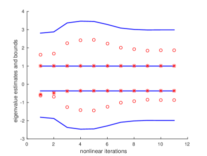
(a) $\lambda(({\cal P}_{aug}^{BDF})^{-1}J^{aug})$

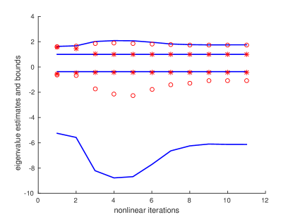
(b) $\lambda(({\cal P}_{red}^{BDF})^{-1}J^{red})$

Figure 1: Eigenvalues of the preconditioned matrices and bounds provided in Theorem 5 versus number of nonlinear iterations (CD problem, $\alpha=10^{-4},\beta=10^{-4}$).

The following result provides spectral information when the indefinite preconditioner is applied to both formulations.

Proposition 6.

The following results hold.

i) Let $\lambda$ be an eigenvalue of $({\cal P}_{aug}^{IPF})^{-1}J^{aug}$. Then $\lambda\in\{1\}\cup[\frac{1}{2},\zeta^{2}+(1+\zeta)^{2}]$. Moreover, there are at least $3n+|{\cal A}|-2|\Pi_{\cal I}|$ eigenvalues equal to $1$. ii) Let $\lambda$ be an eigenvalue of $({\cal P}_{red}^{IPF})^{-1}J^{red}$. Then $\lambda\in\{1\}\cup[\frac{1}{2},\zeta^{2}+(1+\zeta)^{2}]$. Moreover, there are at least $2n-2|\Pi_{\cal I}|$ eigenvalues equal to $1$.

Proof.

i) Explicit computation shows that

$$({\cal P}^{IPF})^{-1}J=\begin{bmatrix}I&J_{11}^{-1}J_{12}^{T}(I-\widehat{S}^{-1}S)\\ 0&\widehat{S}^{-1}S\end{bmatrix}$$

Since

$$\widehat{S}^{-1}S=\begin{bmatrix}I&0\\ -(\bar{M}\Pi_{\cal A}M^{-1}P_{\cal A}^{T})^{T}&I\end{bmatrix}^{-1}\begin{bmatrix}\widehat{\mathbb{S}}^{-1}{\mathbb{S}}&0\\ 0&I\end{bmatrix}\begin{bmatrix}I&0\\ (-\bar{M}\Pi_{\cal A}M^{-1}P_{\cal A}^{T})^{T}&I\end{bmatrix},$$

the eigenvalues of $\widehat{S}^{-1}S$ are either one, or are the eigenvalues of $\widehat{\mathbb{S}}^{-1}{\mathbb{S}}$, which are contained in the given interval, thanks to Proposition 3.

From Proposition 2 we obtain that $\widehat{\mathbb{S}}^{-1}{\mathbb{S}}-I$ is a low rank matrix, of rank at most $2|\Pi_{\cal I}|$. Therefore, there are $2n+|{\cal A}|+(n-2|\Pi_{\cal I}|)$ unit eigenvalues.

ii) For the first part of the proof we proceed as above, since

$$({\cal P}_{red}^{IPF})^{-1}J_{red}=\begin{bmatrix}I&M^{-1}L^{T}(I-\widehat{S}^{-1}S)\\ 0&\widehat{S}^{-1}S\end{bmatrix}.$$

For the unit eigenvalue counting, we notice that the reduced matrix $({\cal P}_{red}^{IPF})^{-1}J_{red}$ has $n$ unit eigenvalues in the (1,1) block and $n-2|\Pi_{\cal I}|$ unit eigenvalues from the second block, for the same argument as above. ∎

We complete this analysis recalling that for both formulations, the preconditioned matrix $({\cal P}^{IPF})^{-1}J$ is unsymmetric, so that a nonsymmetric iterative solver needs to be used. In this setting, the eigenvalues may not provide all the information required to predict the performance of the solver; we refer the reader to [33] where a more complete theoretical analysis of constraint preconditioning is proposed.

5 Numerical experiments

We implemented the semismooth Newton’s method described in Algorithm 1 using MATLAB^® R2016a (both linear and nonlinear solvers) on an Intel® Xeon® 2.30GHz, 132 GB of RAM.

Within the Newton’s method we employed preconditioned gmres [31] and minres [24] as follows

• ssn-gmres-ipf : gmres and indefinite preconditioner ${\cal P}_{aug}^{IPF}/{\cal P}_{red}^{IPF},$

• ssn-minres-bdf : minres and block diagonal preconditioner ${\cal P}_{aug}^{BDF}/{\cal P}_{red}^{BDF}.$

The application of the Schur complement approximation $\widehat{\mathbb{S}}$ requires solving systems with $(\sqrt{\alpha}L+\bar{M}\Pi_{\mathcal{I}})$. As $L$ here is a discretized PDE operator such solves are quite expensive. We thus replace exact solves by approximate solves using an algebraic multigrid technique (hsl-mi20) [5]. We use the function with a Gauss-Seidel coarse solver, $5$ steps of pre-smoothing, and $3$ V-cycles.

The finite element matrices utilizing the SUPG technique were generated using the deal.II library [2], while standard finite differences are used for the Poisson problem.

We used a “feasible” starting point (see Section 3.2) and used the values $\sigma=0.1$ and $\gamma=10^{-4}$ in the line-search strategy described in Algorithm 1, as suggested in [21]. We used $c=1/\alpha$ in (14) in all runs [34, 17]. Nonlinear iterations are stopped as soon as

$$\|\Theta(x_{k})\|\leq 10^{-6},$$

and a maximum number of 100 iterations is allowed.

In order to implement the “exact” Semismooth Newton’s method described in Section 3.2, we solved the linear systems employing a strict tolerance by setting

$$\eta_{k}=10^{-10},\ k\geq 0.$$ (37)

Table 1 summarizes the notation used for the numerical results. We start by illustrating the performance of the different formulations using (37) for the Poisson problem, which is followed by the results of the convection-diffusion system including a discussion on inexact implementations of Algorithm 1.

parameter	description
$\ell$	discretization level for the Poisson problem
$\beta,\alpha$	values of the regularization parameters
li	average number of linear inner iterations
nli	number of nonlinear outer iterations
cpu	average CPU time of the inner solver (in secs)
tcpu	total CPU time (in secs)
%u=0	the percentage of zero elements in the computed control

Table 1: Legend of symbols for the numerical experiments.

5.1 Poisson problem

The first problem that we consider is the Poisson problem defined over the set $\Omega=(0,1)^{d}$, $d={2,3}$ and $L$ is a discretization of the Laplacian from (2) using standard finite differences. We set the control function bounds to $a=-30$, $b=30$ and define the desired state via

$$y_{d}=\left\{\begin{array}[]{l l}\sin(2\pi x)\sin(2\pi y)\exp(2x)/6&\textnormal{ in }2D\\ \sin(2\pi x)\sin(2\pi y)\sin(2\pi z)\exp(2x)/6&\textnormal{ in }3D.\end{array}\right.$$

In Figure 2 the control $u$ for two values of $\beta$ is displayed.

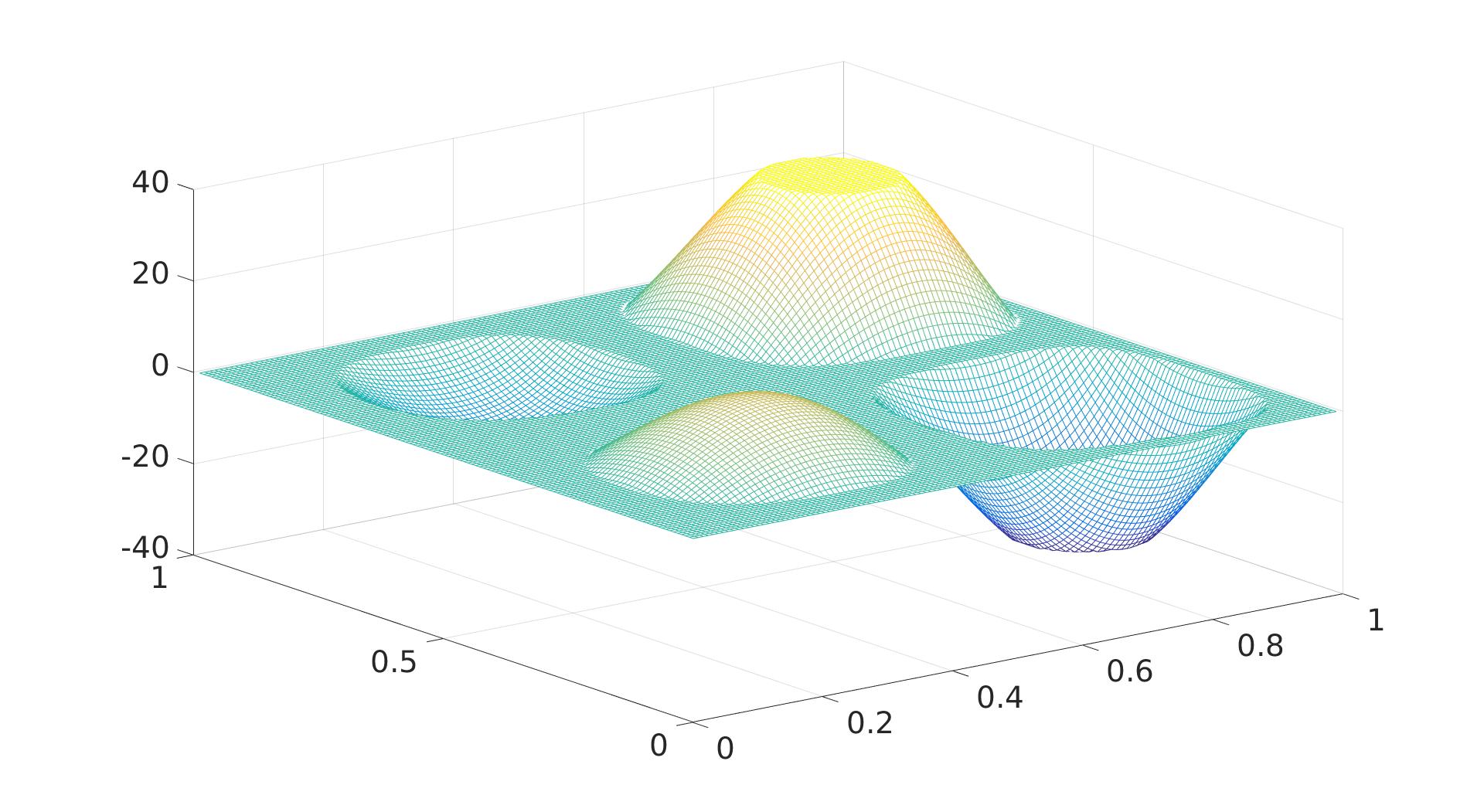
(a) $\beta=10^{-3}$

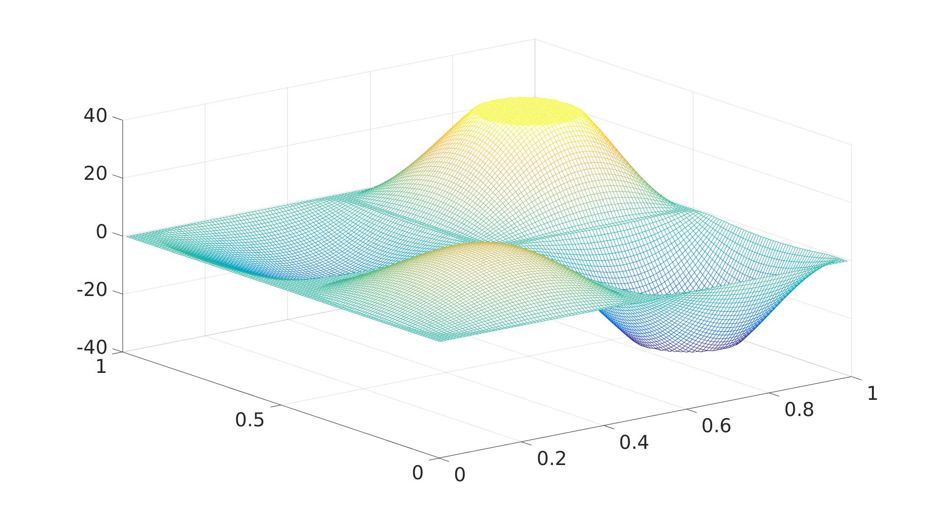
(b) $\beta=10^{-4}$

Figure 2: Control for two different values of the parameter $\beta$.

As we discretize this problem with finite differences we obtain $M=\bar{M}=I$, the identity matrix. The dimension $n$ of control/state vectors is given by $n=(2^{\ell})^{d}$ where $\ell$ is the level of discretization, $d=2,3$. Then, the mesh size is $h=1/(2^{\ell}+1)$. In the 2D case, we tested $\ell=7,8,9$ resulting in $n\in\left\{16384,65536,262144\right\}$; in the 3D case we set $\ell=4,5,6$ yielding $n\in\left\{4096,32768,262144\right\}$ degrees of freedom.

Figure 3 shows that for this problem large values of $\beta$ yield very sparse control $u$ and a large number of nonlinear iterations to find the solution.

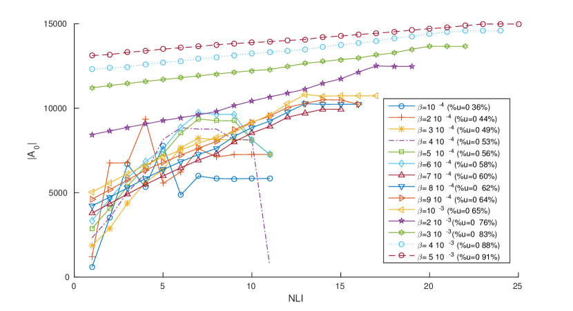
Figure 3: Number of zero components of the control $u$ versus nonlinear iterations, varying $\beta$ (parameters: $\ell=7,\alpha=10^{-6}$).

Table 2 shows the results for two setups applied in the case of the Poisson control problem. The results indicate that the indefinite preconditioner within gmres performs remarkably better in terms of iteration numbers as well as with respect to computing time consumed. Note that the number of (linear) gmres iterations is mesh independent in both formulations, and very mildly dependent on $\alpha$. Moreover, this number is very low for all values of $\alpha$, implying that gmres requires moderate memory requirements, which can be estimated a priori by using information obtained by running the method on a very coarse grid. On this problem the iterative solution of the 2$\times$2 system is not significantly cheaper than that of the 4$\times$4 one. Nonetheless, this slight improvement accumulates during the nonlinear iterations, showing up more significantly in the total CPU time (tcpu), for both preconditioned solvers.

			ssn-gmres-ipf			ssn-minres-bdf
4x4	$\ell$	$\mathrm{log}_{10}\alpha$	li	cpu	tcpu	li	cpu	tcpu	%u=0	nli	bt
	7	-2	11.0	2.0	4.1	25.0	6.0	12.1	3.5	2	0
		-4	16.0	2.9	14.5	34.8	7.8	39.2	8.6	5	0
		-6	27.1	6.2	69.1	61.2	14.0	154.9	35.6	11	9
	8	-2	12.0	7.2	14.4	27.0	19.2	38.5	4.3	2	0
		-4	16.8	8.5	42.6	36.2	25.3	126.9	9.4	5	0
		-6	27.6	16.1	161.9	65.0	44.9	449.5	36.2	10	7
	9	-2	12.0	30.9	61.8	27.0	103.0	206.0	4.7	2	0
		-4	17.2	28.6	143.2	37.0	93.9	469.6	9.7	5	0
		-6	28.8	60.2	782.5	68.7	190.8	2481.5	36.4	13	11
2x2
	7	-2	11.0	2.0	4.0	24.0	4.8	9.6	3.5	2	0
		-4	16.0	2.8	14.1	35.6	6.2	31.3	8.6	5	0
		-6	26.7	5.3	58.9	65.2	11.2	124.0	35.6	11	9
	8	-2	11.5	4.9	9.9	25.0	15.6	31.2	4.3	2	0
		-4	16.4	6.6	33.3	37.0	20.1	100.5	9.4	5	0
		-6	27.5	12.1	121.7	68.3	36.2	362.6	36.2	10	7
	9	-2	12.0	26.0	52.0	25.5	95.2	190.5	4.7	2	0
		-4	17.0	25.9	129.8	38.6	74.4	372.4	9.7	5	0
		-6	28.5	50.6	657.7	71.8	154.4	2007.6	36.4	13	11

Table 2: Results for the Poisson problem with $\beta=10^{-4}$ in two dimensions.

The results in Table 3 show the comparison of our proposed preconditioners for a three-dimensional Poisson problem. The previous results are all confirmed. In particular, it can again be seen that the indefinite preconditioner performs very well in comparison to the block-diagonal one. The timings indicate that the $2\times 2$ formulation is faster than the $4\times 4$ formulation. The matrices stemming from the three-dimensional model are denser, therefore the gain in using the $2\times 2$ formulation is higher.

			ssn-gmres-ipf			ssn-minres-bdf
4x4	$\ell$	$\mathrm{log}_{10}\alpha$	li	cpu	tcpu	li	cpu	tcpu	%u=0	nli	bt
	4	-2	10.0	0.5	1.0	21.0	1.9	3.8	7.4	2	0
		-4	15.3	0.5	2.2	31.5	2.3	9.1	7.6	4	0
		-6	24.0	0.9	7.7	51.1	3.8	30.6	38.6	8	5
	5	-2	10.0	2.5	5.1	23.0	11.7	23.5	8.0	2	0
		-4	16.0	4.2	17.1	33.0	16.5	66.0	13.7	4	0
		-6	29.7	7.6	60.7	62.3	32.6	261.0	44.4	8	2
	6	-2	11.0	19.1	38.2	23.00	82.21	164.41	11.8	2	0
		-4	16.0	27.5	110.1	33.7	121.5	486.2	17.3	4	0
		-6	31.7	71.3	570.5	69.1	261.4	2091.9	46.9	8	2
2x2
	4	-2	10.0	0.3	0.7	20.0	1.2	2.4	7.4	2	0
		-4	14.7	0.5	2.1	32.7	1.8	7.4	7.6	4	0
		-6	23.2	0.8	6.7	53.5	2.8	22.7	38.6	8	5
	5	-2	10.0	2.3	4.7	20.5	8.5	17.1	8.0	2	0
		-4	15.5	3.1	12.7	33.0	12.9	51.9	13.7	4	0
		-6	29.0	6.0	48.4	67.2	26.2	210.1	44.4	8	2
	6	-2	10.5	17.3	34.7	22.0	61.4	122.9	11.8	2	0
		-4	16.0	26.1	104.5	34.7	92.8	371.5	17.3	4	0
		-6	31.2	59.4	475.8	74.5	210.0	1680.3	46.9	8	2

Table 3: Results for the Poisson problem with $\beta=10^{-4}$ in three dimensions.

5.2 Convection diffusion problem

We consider the convection diffusion equation given by

$$\rm-\varepsilon\Delta y+w\cdot\nabla y=u$$

with the wind $\rm w$ defined via $\rm w=(2y(1-x^{2}),-2x(1-y^{2}))$, and the bounds $\rm a=-20$ and $\rm b=20$. We now use finite elements in combination with the streamline upwind Galerkin (SUPG) approach for $\bar{M}$ and $K$ ($n\times n$), which are now nonsymmetric matrices. For our purposes we tested three different mesh-sizes. Namely, $n\in\left\{4225,16641,66049\right\}$ and we also vary the influence of the diffusion by varying $\varepsilon$, i.e., $\varepsilon\in\left\{1,0.5,0.1\right\}$. Figure 4 shows the control $u$ for two values of $\beta$.

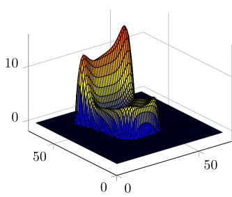
(a) $\beta=5\leavevmode\nobreak\ 10^{-2}$

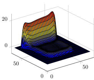
(b) $\beta=10^{-2}$

Figure 4: Control for two different values of the parameter $\beta$.

The results in Table 5 indicate that once more the indefinite preconditioner outperforms the block-diagonal one.

		ssn-gmres-ipf			ssn-minres-bdf
	$\mathrm{log}_{10}\alpha$	li	cpu	tcpu	li	cpu	tcpu	%u=0	nli	bt
$n=4225$	-1	10.0	1.2	2.4	22.0	1.7	3.5	12.0	2	0
$\varepsilon=1$	-2	13.0	1.2	6.0	29.6	2.0	10.0	23.2	5	0
	-3	15.2	1.3	9.3	35.5	2.4	16.7	43.0	7	4
	-4	19.0	1.6	16.3	48.1	3.1	31.3	55.7	10	11
	-5	22.4	2.1	90.4	61.1	3.9	171.0	62.5	43	183
$n=4225$	-1	13.7	1.3	5.4	33.5	2.4	9.7	14.3	4	2
$\varepsilon=1/2$	-2	17.9	1.5	20.5	46.7	3.1	41.4	27.5	13	17
	-3	23.0	2.1	40.6	64.5	4.3	82.0	37.9	19	46
	-4	27.7	2.5	57.5	77.2	5.0	116.5	45.3	23	45
	-5	35.1	3.6	141.8	124.5	8.0	314.9	46.9	39	127
$n=4225$	-1	11.0	1.2	2.4	26.0	1.9	3.8	10.8	2	0
$\varepsilon=1/10$	-2	14.3	1.2	7.2	33.8	2.2	13.3	24.9	6	3
	-3	17.8	1.5	13.5	44.6	2.8	25.9	41.1	9	8
	-4	22.0	2.0	28.2	57.7	3.7	51.7	51.3	14	29
	-5	24.2	2.3	85.1	69.5	4.4	158.9	58.8	36	156
$n=16641$	-1	13.7	5.0	20.2	34.2	9.1	36.4	12.8	4	2
$\varepsilon=1/10$	-2	17.7	6.4	77.6	47.1	12.2	146.8	25.8	12	20
	-3	23.2	8.2	123.6	62.5	17.1	257.7	37.2	15	25
	-4	29.6	11.2	224.5	85.3	21.6	432.9	45.4	20	42
	-5	31.5	15.4	864.3	100.9	25.9	1452.2	48.9	56	369
$n=66049$	-1	13.7	17.7	70.8	34.2	33.7	134.8	12.1	4	2
$\varepsilon=1/10$	-2	18.7	22.7	295.0	50.6	48.5	630.5	25.3	13	18
	-3	23.4	27.0	406.0	63.4	55.2	828.0	36.6	15	24
	-4	32.4	39.7	1231.8	103.3	87.8	2722.4	45.2	31	84
	-5	30.6	42.1	4004.2	98.6	84.3	8010.8	48.9	95	783

Table 4: Convection-Diffusion problem: comparison between ssn-gmres-ipf and ssn-minres-bdf using the $2\times 2$ formulation for various settings (parameters: $\beta=10^{-2}$).

A comparison of both formulations with respect to changes in the mesh-size is shown in Table 5. We see that the performance of the iterative solver for the linear system is robust with respect to changes in the mesh-size but also with respect to the two formulations presented. We also remark that as $\alpha$ gets smaller, the number of back tracking (bt) iterations increases showing that the problem is much harder to solve, and the line-search strategy regularizes the Newton’s model by damping the step. Once again, the reduced formulation is more competitive than the original one.

		ssn-gmres-ipf
$n=16661$	$\mathrm{log}_{10}\alpha$	li	cpu	tcpu	%u=0	nli	bt
$4\times 4$	-1	13.75	5.38	21.52	12.85	4	2
	-2	17.75	6.68	80.18	25.83	12	20
	-3	23.27	9.16	137.35	37.29	15	25
	-4	30.25	13.07	261.45	45.45	20	42
	-5	33.09	17.33	970.60	48.98	56	369
$2\times 2$	-1	13.7	5.0	20.2	12.8	4	2
	-2	17.7	6.4	77.6	25.8	12	20
	-3	23.2	8.2	123.6	37.2	15	25
	-4	29.6	11.2	224.5	45.4	20	42
	-5	31.5	15.4	864.3	48.9	56	369
$n=66049$	$\mathrm{log}_{10}\alpha$	li	cpu	tcpu	%u=0	nli	bt
$4\times 4$	-1	13.75	18.97	75.87	12.16	4	2
	-2	18.77	26.23	340.99	25.39	13	18
	-3	23.47	33.50	502.43	36.64	15	24
	-4	32.48	48.09	1490.65	45.27	31	84
	-5	31.31	53.23	5056.79	48.98	95	783
$2\times 2$	-1	13.7	17.7	70.8	12.1	4	2
	-2	18.7	22.7	295.0	25.3	13	18
	-3	23.4	27.0	406.0	36.6	15	24
	-4	32.4	39.7	1231.8	45.2	31	84
	-5	30.6	42.1	4004.2	48.9	95	783

Table 5: Convection-Diffusion problem: comparison between original and reduced formulations using ssn-gmres-ipf (parameters: $\beta=10^{-2},\varepsilon=1/10$).

We conclude this section discussing the inexact implementation of the Newton’s method. Following the results by Eisenstat and Walker [9] for smooth equations, we chose the so-called adaptive $Choice$ 2 for the forcing term $\eta_{k}$ in (10) in order to achieve the desirable fast local convergence near a solution and, at the same time, to minimize the oversolving: we set

$$\eta_{k}=\chi\left(\frac{\|\Theta_{k+1}\|_{2}}{\|\Theta_{k}\|_{2}}\right)^{2},\,\,k\geq 1,$$ (38)

with $\chi=0.9$ and safeguard

$$\eta_{k}=\max\{\eta_{k},\chi\eta_{k-1}^{2}\},$$

if $\chi\eta_{k-1}^{2}>0.1$; then, the additional safeguard $\eta_{k}=\min\{\eta_{k},\eta_{max}\}$ is used. We considered the values $\eta_{0}=\eta_{max}\in\{10^{-1},10^{-2},10^{-2},10^{-10}\}$ to explore the impact of the linear solver accuracy on the overall Newton’s performance.

In Figure 5, we plot the overall CPU time and the average number of linear iterations varying $\eta_{0}$ for the convection-diffusion problem. These results were obtained using the reduced formulation of the Newton’s equation with the residual test in (26). Nevertheless, we remark that we obtained similar results using the augmented formulation (25), that is the same number of NLI and LI but clearly different values for tcpu.

We note that the gain in CPU time increases for looser accuracy due to the decrease in the linear iterations (almost constant with size). In particular, on average, $\eta_{0}=10^{-1}$ yields a gain of the 65% of tcpu with respect to the “exact” choice $\eta_{0}=10^{-10}$ while the gain with $\eta_{0}=10^{-4}$ is of the 46%.

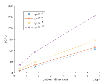
(a) tcpu versus $n$

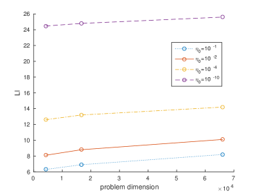
(b) li versus $n$

Figure 5: Convection-diffusion problem. Behavior of the inexact Newton’s method for different values of the parameter $\eta_{0}$ (parameters: $\alpha=10^{-3},\beta=10^{-2},\varepsilon=1/10$).

6 Conclusions

We have presented a general semismooth Newton’s algorithm for the solution of bound constrained optimal control problems where a sparse control is sought. On the one side we have analyzed the nonlinear scheme in the framework of global convergent inexact semismooth Newton methods; on the other side, we have enhanced the solution of the linear algebra phase by proposing reduced formulation of the Newton’s equation and preconditioners based on the active-set Schur complement approximations. We have provided a theoretical support of the proposed techniques and validated the proposals on large scale Poisson and convection-diffusion problems.

References

- [1] O. Axelsson, S. Farouq, and M. Neytcheva, Comparison of preconditioned Krylov subspace iteration methods for PDE-constrained optimization problems, Numer. Algorithms, 73 (2016), pp. 631–663.
- [2] W. Bangerth, R. Hartmann, and G. Kanschat, deal.II—a general-purpose object-oriented finite element library, ACM Trans. Math. Software, 33 (2007), pp. Art. 24, 27.
- [3] M. Benzi, G. Golub, and J. Liesen, Numerical solution of saddle point problems, Acta Numer, 14 (2005), pp. 1–137.
- [4] M. Bergounioux, K. Ito, and K. Kunisch, Primal-dual strategy for constrained optimal control problems, SIAM J. Control Optim., 37 (1999), pp. 1176–1194.
- [5] J. Boyle, M. D. Mihajlović, and J. Scott, HSL_MI20: an efficient AMG preconditioner for finite element problems in 3D, Int. J. Numer. Meth. Engnrg,, 82 (2010), pp. 64–98.
- [6] A. Brooks and T. Hughes, Streamline upwind/Petrov-Galerkin formulations for convection dominated flows with particular emphasis on the incompressible Navier-Stokes equations, Computer methods in applied mechanics and engineering, 32 (1982), pp. 199–259.
- [7] E. J. Candès and M. B. Wakin, An introduction to compressive sampling, IEEE Signal Processing Magazine, 25 (2008), pp. 21–30.
- [8] D. L. Donoho, Compressed sensing, IEEE Trans. Inform. Theory, 52 (2006), pp. 1289–1306.
- [9] S. Eisenstat and H. Walker, Choosing the forcing terms in an inexact Newton method, SIAM Journal on Scientific Computing, 17 (1996), pp. 16–32.
- [10] H. Elman, D. Silvester, and A. Wathen, Finite elements and fast iterative solvers: with applications in incompressible fluid dynamics, Oxford University Press, 2014.
- [11] S. Ganguli and H. Sompolinsky, Compressed sensing, sparsity, and dimensionality in neuronal information processing and data analysis, Annual Review of Neuroscience, 35 (2012), pp. 485–508.
- [12] A. Günnel, R. Herzog, and E. Sachs, A note on preconditioners and scalar products for Krylov methods in Hilbert space, Electronic Transactions on Numerical Analysis, 40 (2014), pp. 13–20.
- [13] M. Heinkenschloss and D. Leykekhman, Local error estimates for SUPG solutions of advection-dominated elliptic linear-quadratic optimal control problems, SIAM Journal on Numerical Analysis, 47 (2010), pp. 4607–4638.
- [14] R. Herzog, J. Obermeier, and G. Wachsmuth, Annular and sectorial sparsity in optimal control of elliptic equations, Computational Optimization and Applications, 62 (2015), pp. 157–180.
- [15] R. Herzog and E. Sachs, Preconditioned conjugate gradient method for optimal control problems with control and state constraints, SIAM J. Matrix Anal. Appl., 31 (2010), pp. 2291–2317.
- [16] R. Herzog, G. Stadler, and G. Wachsmuth, Directional sparsity in optimal control of partial differential equations., SIAM J. Control Optim., 50 (2012), pp. 943–963.
- [17] M. Hintermüller, K. Ito, and K. Kunisch, The primal-dual active set strategy as a semismooth Newton method, SIAM J. Optim., 13 (2002), pp. 865–888.
- [18] M. Hinze, R. Pinnau, M. Ulbrich, and S. Ulbrich, Optimization with PDE Constraints, Mathematical Modelling: Theory and Applications, Springer-Verlag, New York, 2009.
- [19] K. Ito and K. Kunisch, Lagrange multiplier approach to variational problems and applications, vol. 15 of Advances in Design and Control, Society for Industrial and Applied Mathematics (SIAM), Philadelphia, PA, 2008.
- [20] K. Mardal and R. Winther, Construction of preconditioners by mapping properties, Bentham Science Publishers, 2010, ch. 4, pp. 65–84.
- [21] J. Martínez and L. Qi, Inexact newton methods for solving nonsmooth equations, Journal of Computational and Applied Mathematics, 60 (1995), pp. 127–145.
- [22] J. Nakamura, Image sensors and signal processing for digital still cameras, CRC press, 2016.
- [23] J. Nocedal and S. Wright, Numerical optimization, Springer Series in Operations Research and Financial Engineering, Springer, New York, second ed., 2006.
- [24] C. C. Paige and M. A. Saunders, Solutions of sparse indefinite systems of linear equations, SIAM J. Numer. Anal, 12 (1975), pp. 617–629.
- [25] J. W. Pearson and A. Wathen, A new approximation of the Schur complement in preconditioners for PDE-constrained optimization, Numerical Linear Algebra with Applications, 19 (2012), pp. 816–829.
- [26] J. W. Pearson and A. J. Wathen, Fast iterative solvers for convection-diffusion control problems, Electronic Transactions on Numerical Analysis, 40 (2013), pp. 294–310.
- [27] I. Perugia and V. Simoncini, Block–diagonal and indefinite symmetric preconditioners for mixed finite element formulations, Numerical Linear Algebra with Applications, 7 (2000), pp. 585–616.
- [28] M. Porcelli, V. Simoncini, and M. Tani, Preconditioning of active-set Newton methods for PDE-constrained optimal control problems, SIAM Journal on Scientific Computing, 37 (2015), pp. S472–S502.
- [29] T. Rees, Preconditioning Iterative Methods for PDE Constrained Optimazation, PhD thesis, University of Oxford, 2010.
- [30] Y. Saad, Iterative methods for sparse linear systems, Society for Industrial and Applied Mathematics, Philadelphia, PA, 2003.
- [31] Y. Saad and M. Schultz, GMRES: a generalized minimal residual algorithm for solving nonsymmetric linear systems, SIAM J. Sci. Statist. Comput, 7 (1986), pp. 856–869.
- [32] A. Schiela and S. Ulbrich, Operator Preconditioning for a Class of Constrained Optimal Control Problems, SIAM J. Optim., 24 (2012), pp. 435–466.
- [33] D. Sesana and V. Simoncini, Spectral analysis of inexact constraint preconditioning for symmetric saddle point matrices, Linear Algebra and its Applications, 438 (2013), pp. 2683–2700.
- [34] G. Stadler, Elliptic optimal control problems with -control cost and applications for the placement of control devices., Comput. Optim. Appl., 44 (2009), pp. 159–181.
- [35] M. Stoll, J. W. Pearson, and A. Wathen, Preconditioners for state constrained optimal control problems with Moreau-Yosida penalty function, Numer. Lin. Alg. Appl., 21 (2014), pp. 81–97.
- [36] T. Sun, Discontinuous galerkin finite element method with interior penalties for convection diffusion optimal control problem, Int. J. Numer. Anal. Mod, 7 (2010), pp. 87–107.
- [37] F. Tröltzsch, Optimal Control of Partial Differential Equations: Theory, Methods and Applications, Amer Mathematical Society, 2010.
- [38] M. Ulbrich, Semismooth Newton Methods for Variational Inequalities and Constrained Optimization Problems, SIAM Philadelphia, 2011.