Second-order transport, quasinormal modes and zero-viscosity limit in the Gauss-Bonnet holographic fluid

Abstract

Gauss-Bonnet holographic fluid is a useful theoretical laboratory to study the effects of curvature-squared terms in the dual gravity action on transport coefficients, quasinormal spectra and the analytic structure of thermal correlators at strong coupling. To understand the behavior and possible pathologies of the Gauss-Bonnet fluid in $3+1$ dimensions, we compute (analytically and non-perturbatively in the Gauss-Bonnet coupling) its second-order transport coefficients, the retarded two- and three-point correlation functions of the energy-momentum tensor in the hydrodynamic regime as well as the relevant quasinormal spectrum. The Haack-Yarom universal relation among the second-order transport coefficients is violated at second order in the Gauss-Bonnet coupling. In the zero-viscosity limit, the holographic fluid still produces entropy, while the momentum diffusion and the sound attenuation are suppressed at all orders in the hydrodynamic expansion. By adding higher-derivative electromagnetic field terms to the action, we also compute corrections to charge diffusion and identify the non-perturbative parameter regime in which the charge diffusion constant vanishes.

1 Introduction

Gauge-string duality has been applied successfully to explore qualitative, quantitative and conceptual issues in fluid dynamics Son:2007vk ; Baier:2007ix ; Rangamani:2009xk ; Banerjee:2012iz ; Jensen:2012jh ; Kovtun:2012rj ; Crossley:2015tka ; Haehl:2015pja ; Haehl:2016pec ; Haehl:2016uah . Although the number of quantum field theories with known dual string (gravity) descriptions is very limited, their transport and spectral function properties at strong coupling can in principle be fully determined, thus giving valuable insights into the behavior of strongly interacting quantum many-body systems. Moreover, dual gravity methods can be used to determine coupling constant dependence of a variety of physical quantities with an ultimate goal of interpolating between weak and strong coupling results and describing, at least qualitatively, the intermediate coupling behavior in theories of phenomenological interest Romatschke:2015gic ; Grozdanov:2016vgg ; Heller:2016rtz ; Heller:2016gbp ; Grozdanov:2016zjj ; Andrade:2016rln .

For generic neutral fluids, there are two independent first-order transport coefficients (shear viscosity $\eta$ and bulk viscosity $\zeta$), and fifteen second-order coefficients (see e.g. Romatschke:2009im ). For Weyl-invariant or "conformal" fluids, the additional symmetry constraints reduce the number of transport coefficients to one at first order (shear viscosity $\eta$) and five at second order (usually denoted $\tau_{\Pi}$, $\kappa$, $\lambda_{1}$, $\lambda_{2}$, $\lambda_{3}$). The coefficients $\eta$, $\tau_{\Pi}$, $\lambda_{1}$, $\lambda_{2}$ are "dynamical", whereas $\kappa$ and $\lambda_{3}$ are "thermodynamical" in the classification introduced in ref. Moore:2012tc . In the parameter regime where the dual Einstein gravity description of conformal fluids is applicable (e.g. at infinite ’t Hooft coupling $\lambda=g^{2}_{YM}N_{c}$ and infinite $N_{c}$ in theories such as ${\cal N}=4$ $SU(N_{c})$ supersymmetric Yang-Mills (SYM) theory in $d=3+1$ dimensions), the six transport coefficients (in $d$ space-time dimensions, $d>2$) are given by Bhattacharyya:2008mz

$$\eta_{\;} = s/4\pi\,,$$ (1)

$$\tau_{\Pi} = \frac{d}{4\pi T}\left(1+\frac{1}{d}\left[\gamma_{E}+\psi\left(\frac{2}{d}\right)\right]\right)\,,$$ (2)

$$\kappa_{\;} = \frac{d}{d-2}\,\frac{\eta}{2\pi T}\,,$$ (3)

$$\lambda_{1} = \frac{d\eta}{8\pi T}\,,$$ (4)

$$\lambda_{2} = \left[\gamma_{E}+\psi\left(\frac{2}{d}\right)\right]\,\frac{\eta}{2\pi T}\,,$$ (5)

$$\lambda_{3} = 0\,,$$ (6)

where $s$ is the entropy density, $\psi(z)$ is the logarithmic derivative of the gamma function, and $\gamma_{E}$ is the Euler-Mascheroni constant. Generically, one expects corrections to these formulas in (inverse) powers of the parameters such as $\lambda$ and $N_{c}$. For ${\cal N}=4$ SYM at finite temperature, the leading $\lambda^{-3/2}$ corrections to all six coefficients are known Buchel:2004di ; Benincasa:2005qc ; Buchel:2008sh ; Buchel:2008ac ; Buchel:2008bz ; Buchel:2008kd ; Saremi:2011nh ; Grozdanov:2014kva (see Appendix A, where weak and strong coupling results are discussed). Other coupling constant corrections to the results at infinitely strong t’Hooft coupling in this theory include corrections to the entropy Gubser:1998nz ; Pawelczyk:1998pb , photon emission rate Hassanain:2012uj , and poles of the retarded correlators of the energy-momentum tensor Stricker:2013lma ; Waeber:2015oka ; Grozdanov:2016vgg . Leading corrections in $1/N_{c}^{2}$, intimately related to the issue of hydrodynamic "long time tails", were discussed in refs. Kovtun:2003vj ; CaronHuot:2009iq ; Kovtun:2011np , and in refs. Myers:2008yi ; Buchel:2008ae .

In the regime of strong coupling, theories with gravity dual description appear to exhibit robust properties of transport coefficients and relations among them. One of such properties is the universality of shear viscosity to entropy density ratio $\eta/s=1/4\pi$ in the limit described by a dual gravity with two-derivative action Kovtun:2004de , Buchel:2004qq , Kovtun:2003wp ; Buchel:2003tz ; Starinets:2008fb . Another one seems to be the Haack-Yarom relation: following the observation in ref. Erdmenger:2008rm , the linear combination of the second-order transport coefficients

$$H\equiv 2\eta\tau_{\Pi}-4\lambda_{1}-\lambda_{2}$$ (7)

was proven to vanish in all conformal theories dual to two-derivative gravity Haack:2008xx . Eqs.  (2), (4), (5) show this explicitly. Somewhat surprisingly, the Haack-Yarom relation continues to hold to next to leading order in the strong coupling expansion, at least in ${\cal N}=4$ $SU(N_{c})$ supersymmetric Yang-Mills theory in $d=3+1$ dimensions in the limit of infinite $N_{c}$ Grozdanov:2014kva , in theories dual to curvature-squared gravity Grozdanov:2014kva , in particular, in the Gauss-Bonnet holographic liquid (perturbatively in the Gauss-Bonnet coupling) Shaverin:2012kv . It was shown recently that the result $H=0$ continues to hold for non-conformal liquids along the dual gravity RG flow Kleinert:2016nav . It remains to be seen whether such robustness extends to higher-order transport coefficients and/or other properties of strongly coupled finite temperature theories and whether it is related to the presence of event horizons in dual gravity.

Monotonicity and other properties of transport coefficients are of interest for studies of near-equilibrium behavior at strong coupling, in particular, thermalization, and for attempts to uncover a universality similar to the one exhibited by the ratio of shear viscosity to entropy density. Monotonicity of transport coefficients or their dimensionless combinations may seem more exotic than the monotonicity of central charges Zamolodchikov:1986gt ; Komargodski:2011vj or the free energy Klebanov:2011gs ; Pufu:2016zxm , yet it is often an observed property, at least in a given state of aggregation Kovtun:2004de ; Csernai:2006zz .

In ${\cal N}=4$ SYM at infinite $N_{c}$, the shear viscosity to entropy density ratio appears to be a monotonic function of the coupling Kovtun:2004de , with the correction to the universal infinite coupling result being positive Buchel:2004di ; Buchel:2008sh ,

$$\frac{\eta}{s}=\frac{1}{4\pi}\left(1+15\zeta(3)\lambda^{-3/2}+\ldots\right)\,.$$ (8)

Subsequent calculations revealed that the corrections coming from higher derivative terms in the gravitational action can have either sign Kats:2007mq ; Brigante:2007nu . For the action with generic curvature squared higher derivative terms

$$S_{R^{2}}=\frac{1}{2\kappa_{5}^{2}}\int d^{5}x\sqrt{-g}\left[R-2\Lambda+L^{2}\left(\alpha_{1}R^{2}+\alpha_{2}R_{\mu\nu}R^{\mu\nu}+\alpha_{3}R_{\mu\nu\rho\sigma}R^{\mu\nu\rho\sigma}\right)\right],$$ (9)

where the cosmological constant $\Lambda=-6/L^{2}$, the shear viscosity - entropy density ratio is Kats:2007mq ; Brigante:2007nu

$$\frac{\eta}{s}=\frac{1}{4\pi}\left(1-8\alpha_{3}\right)+O\left(\alpha_{i}^{2}\right).$$ (10)

The sign of the coefficient $\alpha_{3}$ affects not only viscosity but also the analytic structure of correlators in the dual thermal field theory Grozdanov:2016vgg .

Corrections to Einstein gravity results computed from generic higher-order derivative terms in the dual gravitational action can be trusted so long as they remain (infinitesimally) small relative to the leading order result, as they are obtained by treating the higher-derivative terms in the equations of motion perturbatively. This limitation arises due to Ostrogradsky instability and other related pathologies such as ghosts associated with higher-derivative actions Ostrogradsky , pais , Stelle:1977ry , Zwiebach:1985uq (see also refs. Woodard:2006nt , Woodard:2015zca for a modern discussion of Ostrogradsky’s theorem, and ref. ostrogradsky-bio for an interesting historical account of Ostrogradsky’s life and work). One may be tempted to lift the constraints imposed by Ostrogradsky’s theorem by considering actions in which coefficients in front of higher derivative terms conspire to give equations of motion no higher than second-order in derivatives as happens e.g. in Gauss-Bonnet gravity in dimension $D>4$ or, more generally, Lovelock gravity Lovelock:1971yv . Gauss-Bonnet (and Lovelock) gravity has been used as a laboratory for non-perturbative studies of higher derivative curvature effects on transport coefficients of conformal fluids with holographic duals Kats:2007mq ; Brigante:2007nu ; Brigante:2008gz ; Buchel:2009tt ; Buchel:2009sk ; deBoer:2009gx ; Camanho:2009hu ; Camanho:2010ru ; Camanho:2013pda , Grozdanov:2016vgg . In particular, the celebrated result for the shear viscosity-entropy ratio in a (hypothetical) conformal fluid dual to $D=5$ Gauss-Bonnet gravity Brigante:2007nu ,

$$\frac{\eta}{s}=\frac{1-4\lambda_{\scriptscriptstyle GB}}{4\pi},$$ (11)

has been obtained non-perturbatively in the Gauss-Bonnet coupling $\lambda_{\scriptscriptstyle GB}$. The result would imply that there exist CFTs whose viscosity can be tuned all the way to zero in the regime described by a dual classical (albeit non-Einsteinian) gravity. It was found, however, that for $\lambda_{\scriptscriptstyle GB}$ outside of the interval

$$-\frac{7}{36}\leq\lambda_{\scriptscriptstyle GB}\leq\frac{9}{100},$$ (12)

the dual field theory exhibits pathologies associated with superluminal propagation of modes at high momenta or negativity of the energy flux in a dual CFT Brigante:2007nu ; Brigante:2008gz ; Hofman:2008ar ; Buchel:2009tt ; Hofman:2009ug ; Buchel:2009sk . For Gauss-Bonnet gravity in $D$ dimensions ($D\geq 5$), the result (11) generalizes to Camanho:2009vw ; Buchel:2009sk

$$\frac{\eta}{s}=\frac{1}{4\pi}\left[1-\frac{2(D-1)}{D-3}\lambda_{\scriptscriptstyle GB}\right]$$ (13)

and the inequalities corresponding to eq. (12) become Camanho:2009vw ; Buchel:2009sk

$$-\frac{(3D-1)(D-3)}{4(D+1)^{2}}\leq\lambda_{\scriptscriptstyle GB}\leq\frac{(D-3)(D-4)(D^{2}-3D+8)}{4(D^{2}-5D+10)^{2}}\,.$$ (14)

Given the constraints (14) and monotonicity of $\eta/s$ in (13), one may conjecture a GB gravity bound on $\eta/s$ Camanho:2009vw ; Buchel:2009sk ,

$$\frac{\eta}{s}\geq\frac{1}{4\pi}\left[1-\frac{(D-1)(D-4)(D^{2}-3D+8)}{2(D^{2}-5D+10)^{2}}\right],$$ (15)

instead of the Einstein’s gravity bound $\eta/s\geq 1/4\pi$. For $3+1$-dimensional CFTs, the GB bound would imply $\eta/s\geq(0.640)/4\pi$ Brigante:2008gz . Recently, the constraints (12) were confirmed and generalized to Gauss-Bonnet black holes with spherical (rather than planar) horizons by considering boundary causality and bulk hyperbolicity violations in Einstein-Gauss-Bonnet gravity Andrade:2016yzc . Since these causality problems arise in the ultraviolet, one may hope that treating Gauss-Bonnet gravity as a low energy theory with unspecified ultraviolet completion would allow one to consider its hydrodynamic (infrared) limit without worrying about causality violating ultraviolet modes, i.e. that it is in principle possible to cure the problems in the ultraviolet without affecting the hydrodynamic (infrared) regime (one may also try to construct a theory with a low temperature phase transition breaking the link between the hydrodynamic IR and causality breaking UV modes Buchel:2010wf ). However, a reflection on the recent analysis by Camanho et al. Camanho:2014apa of the bulk causality violation in higher derivative gravity seems to imply that, provided the relevant conclusions of ref. Camanho:2014apa are correct, a reliable treatment of Gauss-Bonnet terms beyond perturbation theory for the purposes of fluid dynamics is not possible. The Einstein-Gauss-Bonnet action in $D=5$ is given by

$$S_{GB}=\frac{1}{2\kappa_{5}^{2}}\int d^{5}x\sqrt{-g}\left[R-2\Lambda+\frac{\lambda_{\scriptscriptstyle GB}l_{\scriptscriptstyle GB}^{2}}{2}\left(R^{2}-4R_{\mu\nu}R^{\mu\nu}+R_{\mu\nu\rho\sigma}R^{\mu\nu\rho\sigma}\right)\right],$$ (16)

where the cosmological constant $\Lambda=-6/L^{2}$, and $l_{GB}$ is the scale of the Gauss-Bonnet term which a priori is not necessarily related to the cosmological constant scale set by $L$. As argued in ref. Camanho:2014apa , the generic bulk causality violations in Gauss-Bonnet classical gravity can only be cured by including an infinite set of higher spin fields with masses squared $m_{s}^{2}\propto 1/\lambda_{\scriptscriptstyle GB}l_{\scriptscriptstyle GB}^{2}$. Integrating out these fields to obtain a low energy effective theory would lead to an infinite series of additional higher derivative terms in the gravitation action. Schematically, the modified action would have the form

$$S_{GB,mod}=\frac{1}{2\kappa_{5}^{2}}\int d^{5}x\sqrt{-g}\left[R-2\Lambda+\sum\limits_{k=1}^{\infty}c_{k}\,\lambda_{\scriptscriptstyle GB}^{k}\,l_{\scriptscriptstyle GB}^{2k}\,{\cal R}^{k+1}\right].$$ (17)

Considering a specific solution (e.g. a black brane whose scale is set by the cosmological constant) and rescaling the coordinates $x\rightarrow\bar{x}=x/L$ leads to

$$S_{GB,mod}=\frac{L^{3}}{2\kappa_{5}^{2}}\int d^{5}\bar{x}\sqrt{-\bar{g}}\left[\bar{R}+12+\sum\limits_{k=1}^{\infty}c_{k}\,\bar{\lambda}_{\scriptscriptstyle GB}^{k}\,\bar{{\cal R}}^{k+1}\right],$$ (18)

where $\bar{\lambda}_{\scriptscriptstyle GB}=\lambda_{\scriptscriptstyle GB}l_{\scriptscriptstyle GB}^{2}/L^{2}$. To suppress contributions (e.g. to transport coefficients) coming from the (unknown) terms with $k>1$, one has to assume $\bar{\lambda}_{\scriptscriptstyle GB}\ll 1$. This is similar to the condition $l_{s}/L\ll 1$ in the usual top-down holography. Thus, generically one may expect results such as (11) to be potentially corrected by terms $O(\lambda_{\scriptscriptstyle GB}^{2})$ and/or higher, and therefore be reliable only for $\lambda_{\scriptscriptstyle GB}\ll 1$. It seems, therefore, that one essentially cannot escape the Ostrogradsky problem (at least not in classical gravity) by engineering a specific higher-derivative Lagrangian with second-order equations of motion. An alternative view of the aspects of the analysis in ref. Camanho:2014apa has been advocated in refs. Reall:2014pwa ; Papallo:2015rna (see also Willison:2014era ; Willison:2015vaa and Andrade:2016yzc ). Our approach to these problems will be purely pragmatic: we shall a priori ignore any existing or debated constraints on the Gauss-Bonnet coupling and explore the influence of curvature-squared terms on quasinormal spectra and transport coefficients for all range of the coupling allowing a black brane solution, i.e. for $\lambda_{\scriptscriptstyle GB}\in(-\infty,1/4]$ (see section 2). In particular, we are interested in revealing any generic features the presence of higher-curvature terms in the action may have (as pointed out in ref. Grozdanov:2016vgg , the spectra of $R^{2}$ and $R^{4}$ backgrounds exhibit qualitatively similar novel features not present in Einstein’s gravity). We use the action (16) (with $l_{\scriptscriptstyle GB}=L$) to compute transport coefficients, quasinormal spectrum and thermal correlators analytically and non-perturbatively in Gauss-Bonnet coupling, fully exploiting the advantage of having to deal with second-order equations of motion in the bulk. Different techniques will be used to compute Gauss-Bonnet transport: fluid-gravity duality, Kubo formulae applied to two- and three-point correlators, and quasinormal modes. We find that only the three-point functions method allows to determine all the coefficients analytically: other approaches face technical difficulties we were not able to resolve. In a hypothetical dual CFT, constraints on Gauss-Bonnet coupling considered e.g. in ref. Buchel:2009sk manifest themselves in the superluminal propagation of high-momentum modes for $\lambda_{\scriptscriptstyle GB}$ outside of the interval (14). In the far more stringent scenario of ref. Camanho:2014apa , one may expect to detect anomalous behavior in the regime of small frequencies and momenta and in transport coefficients. Accordingly, we shall look for pathologies in the hydrodynamic behavior of the model at finite values of $\lambda_{\scriptscriptstyle GB}$ indicating the lack of ultraviolet completion and the potential need for corrections coming from the unknown terms in (18).

The full non-perturbative set of first- and second-order Gauss-Bonnet transport coefficients can be determined analytically and is given by

$$\eta=s\gamma_{\scriptscriptstyle GB}^{2}/4\pi\,,$$ (19)

$$\tau_{\Pi}=\frac{1}{2\pi T}\left(\frac{1}{4}\left(1+\gamma_{\scriptscriptstyle GB}\right)\left(5+\gamma_{\scriptscriptstyle GB}-\frac{2}{\gamma_{\scriptscriptstyle GB}}\right)-\frac{1}{2}\ln\left[\frac{2\left(1+\gamma_{\scriptscriptstyle GB}\right)}{\gamma_{\scriptscriptstyle GB}}\right]\right),$$ (20)

$$\kappa=\frac{\eta}{\pi T}\left(\frac{\left(1+\gamma_{\scriptscriptstyle GB}\right)\left(2\gamma_{\scriptscriptstyle GB}^{2}-1\right)}{2\gamma_{\scriptscriptstyle GB}^{2}}\right)\,,$$ (21)

$$\lambda_{1}=\frac{\eta}{2\pi T}\left(\frac{\left(1+\gamma_{\scriptscriptstyle GB}\right)\left(3-4\gamma_{\scriptscriptstyle GB}+2\gamma_{\scriptscriptstyle GB}^{3}\right)}{2\gamma_{\scriptscriptstyle GB}^{2}}\right),$$ (22)

$$\lambda_{2}=-\frac{\eta}{\pi T}\left(-\frac{1}{4}\left(1+\gamma_{\scriptscriptstyle GB}\right)\left(1+\gamma_{\scriptscriptstyle GB}-\frac{2}{\gamma_{\scriptscriptstyle GB}}\right)+\frac{1}{2}\ln\left[\frac{2\left(1+\gamma_{\scriptscriptstyle GB}\right)}{\gamma_{\scriptscriptstyle GB}}\right]\right),$$ (23)

$$\lambda_{3}=-\frac{\eta}{\pi T}\left(\frac{\left(1+\gamma_{\scriptscriptstyle GB}\right)\left(3+\gamma_{\scriptscriptstyle GB}-4\gamma_{\scriptscriptstyle GB}^{2}\right)}{\gamma_{\scriptscriptstyle GB}^{2}}\right),$$ (24)

where we have defined

$$\gamma_{\scriptscriptstyle GB}\equiv\sqrt{1-4\lambda_{\scriptscriptstyle GB}}\,.$$ (25)

An alternative way of writing the Gauss-Bonnet second-order coefficients is given by Eqs. (173) – (177). In the limit of $\lambda_{\scriptscriptstyle GB}\rightarrow 0$ ($\gamma_{\scriptscriptstyle GB}\rightarrow 1$), which corresponds to Einstein’s gravity, one recovers the standard results for infinitely strongly coupled conformal fluids in $3+1$ dimensions given by eqs. (202) and (203) in appendix A. The result for $\eta$ was obtained in ref. Brigante:2007nu and the relaxation time $\tau_{\Pi}$ was first found numerically in ref. Buchel:2009tt . Coefficients $\tau_{\Pi}$ and $\kappa$ were previously computed analytically in ref. Banerjee:2011tg , and we have reported $\lambda_{1}$, $\lambda_{2}$, $\lambda_{3}$ in ref. Grozdanov:2015asa . To linear order in $\lambda_{\scriptscriptstyle GB}$, the results coincide with those found in ref. Shaverin:2012kv .

Using the results (19), (20), (22), (23), we find the Haack-Yarom function in Gauss-Bonnet gravity

$$H(\lambda_{\scriptscriptstyle GB})=-\frac{\eta}{\pi T}\frac{\left(1-\gamma_{\scriptscriptstyle GB}\right)\left(1-\gamma_{\scriptscriptstyle GB}^{2}\right)\left(3+2\gamma_{\scriptscriptstyle GB}\right)}{\gamma_{\scriptscriptstyle GB}^{2}}=-\frac{40\lambda_{\scriptscriptstyle GB}^{2}\eta}{\pi T}\,+\mathcal{O}\left(\lambda_{\scriptscriptstyle GB}^{3}\right).$$ (26)

Curiously, $H(\lambda_{\scriptscriptstyle GB})\leq 0$ for the Gauss-Bonnet holographic liquid. Whether $H(\lambda_{\scriptscriptstyle GB})$ is corrected beyond leading order by terms coming from (18) remains an open question: a priori, we do not know if $H$ must vanish beyond the Einstein gravity approximation.

Computing the energy-momentum tensor correlation functions in holographic models with higher-derivative dual gravity terms, one finds a new pole on the imaginary frequency axis. This pole, first found in the quasinormal spectrum analysis of ref. Grozdanov:2016vgg , is moving from the complex infinity closer and closer to the origin as the parameter in front of the higher-derivative term in the action (such as $\lambda_{\scriptscriptstyle GB}$ in eq. (16)) increases, and can be approximated analytically in the small-frequency expansion. The poles of this type appear to be generic in higher-derivative gravity: they are present in $R^{2}$ and $R^{4}$ gravity, and their behavior is qualitatively similar Grozdanov:2016vgg .

Another interesting feature of Gauss-Bonnet holographic liquid is the zero-viscosity limit. In ref. Bhattacharya:2012zx , Bhattacharya et al. suggested the existence of a non-trivial second-order non-dissipative hydrodynamics, i.e. a theory whose fluid dynamics derivative expansion has no contribution to entropy production while still having some of the transport coefficients non-vanishing. For conformal fluids, the classification of Bhattacharya:2012zx implies the existence of a four-parameter family of non-trivial non-dissipative fluids with $\eta=0$ and non-vanishing coefficients $\tau_{\Pi}$, $\kappa$, $\lambda_{1}=\kappa/2$, $\lambda_{2}$ and $\lambda_{3}$. Given the result (11), the hypothetical theory dual to Gauss-Bonnet gravity in the limit of $\lambda_{\scriptscriptstyle GB}\rightarrow 1/4$ is a natural candidate for a dissipationless fluid (ignoring for a moment any potential corrections coming from (18)). In the limit of $\lambda_{\scriptscriptstyle GB}\rightarrow 1/4$ ($\gamma_{\scriptscriptstyle GB}\rightarrow 0$) we find Grozdanov:2015asa

$$\eta\tau_{\Pi}=0, \lambda_{1}=\frac{3\pi^{2}T^{2}}{2\sqrt{2}\kappa_{5}^{2}}, \lambda_{2}=0, \lambda_{3}=-\frac{3\sqrt{2}\pi^{2}T^{2}}{\kappa_{5}^{2}}, \kappa=-\frac{\pi^{2}T^{2}}{\sqrt{2}\kappa_{5}^{2}}.$$ (27)

At first glance, this result realizes the dissipationless liquid scenario outlined in ref. Bhattacharya:2012zx : the shear and bulk viscosities are zero while some of the second-order coefficients are not. However, the relationship $\kappa=2\lambda_{1}$, which is required for ensuring zero entropy production, does not hold among the coefficients in (27). We therefore conclude that the holographic Gauss-Bonnet liquid does not fall into the class of non-dissipative liquids discussed in ref. Bhattacharya:2012zx . This may be a hint that the corrections from (18) must indeed be included.

The paper is organised as follows. In section 2 we analyze the finite-temperature two-point correlation functions of energy-momentum tensor in the theory dual to Gauss-Bonnet gravity as well as the relevant quasinormal modes in the scalar, shear and sound channels of metric perturbations, including the new pole on the imaginary axis at finite coupling $\lambda_{\scriptscriptstyle GB}$. Kubo formulas determine the coefficients $\eta$, $\kappa$ and $\tau_{\Pi}$. The shear channel quasinormal frequency is used to confirm the results for $\eta$ and $\tau_{\Pi}$, and to find the third-order transport coefficient $\theta_{1}$. We discuss the limit $\lambda_{\scriptscriptstyle GB}\rightarrow 1/4$, where the full quasinormal spectrum can be found analytically, and the limit $\lambda_{\scriptscriptstyle GB}\rightarrow-\infty$. In section 3, we apply the fluid-gravity duality technique to compute the Gauss-Bonnet transport coefficients. All coefficients except $\kappa$ can be determined in this approach. However, due to technical difficulties, all of them with the exception of $\eta$ can be found only perturbatively as series in $\lambda_{\scriptscriptstyle GB}$. A more efficient method of three-point functions is considered in section 4, where all the coefficients are computed analytically and non-perturbatively, and we also discuss the monotonicity properties of the coefficients and the zero-viscosity limit. Finally, in section 5 we discuss the influence of higher derivative terms on charge diffusion in the most general four derivative Einstein-Maxwell theory. Section 6 with conclusions is followed by several appendices: in Appendix A, a brief summary of second-order transport coefficients in ${\cal N}=4$ SYM at weak and strong coupling is given. A comparison of notations and conventions used in the literature on second-order hydrodynamics and, specifically, in the discussion of Haack-Yarom relation is given in Appendix B. In Appendix C we outline the procedure of setting the boundary conditions at the horizon in hydrodynamic approximation. Appendices D and E contain some technical results.

2 Energy-momentum tensor correlators and quasinormal modes of Gauss-Bonnet holographic fluid

The coefficients of the four-derivative terms in the Gauss-Bonnet action (16) ensure that the corresponding equations of motion contain only second derivatives of the metric. The equations are given by

$$E_{\mu\nu}\equiv \;R_{\mu\nu}-\frac{1}{2}g_{\mu\nu}R+g_{\mu\nu}\Lambda-\frac{\lambda_{\scriptscriptstyle GB}L^{2}}{4}g_{\mu\nu}\left(R^{2}-4R_{\mu\nu}R^{\mu\nu}+R_{\mu\nu\rho\sigma}R^{\mu\nu\rho\sigma}\right)$$

$$+\lambda_{\scriptscriptstyle GB}L^{2}\left(RR_{\mu\nu}-2R_{\mu\alpha}R_{\nu}^{~{}\alpha}-2R_{\mu\alpha\nu\beta}R^{\alpha\beta}+R_{\mu\alpha\beta\gamma}R_{\nu}^{\alpha\beta\gamma}\right)=0\,.$$ (28)

The equations (2) admit a black brane solution

$$ds^{2}=-f(r)N^{2}_{GB}dt^{2}+\frac{1}{f(r)}dr^{2}+\frac{r^{2}}{L^{2}}\left(dx^{2}+dy^{2}+dz^{2}\right),$$ (29)

where

$$f(r)=\frac{r^{2}}{L^{2}}\frac{1}{2\lambda_{\scriptscriptstyle GB}}\left[1-\sqrt{1-4\lambda_{\scriptscriptstyle GB}\left(1-\frac{r^{4}_{+}}{r^{4}}\right)}\right].$$ (30)

The arbitrary constant $N_{\scriptscriptstyle GB}$ will be set to normalize the speed of light at the boundary (i.e. in the dual CFT) to unity,

$$N_{\scriptscriptstyle GB}^{2}=\frac{1}{2}\left(1+\sqrt{1-4\lambda_{\scriptscriptstyle GB}}\right),$$ (31)

and we henceforth use this value. The solution with $r_{+}=0$ corresponds to the AdS vacuum metric in Poincaré coordinates with the AdS curvature scale squared $\tilde{L}^{2}=L^{2}/f_{\infty}$ Buchel:2009sk , where

$$f_{\infty}=\lim_{r\rightarrow\infty}f(r)=\frac{1-\sqrt{1-4\lambda_{\scriptscriptstyle GB}}}{2\lambda_{\scriptscriptstyle GB}}=\frac{2}{1+\gamma_{\scriptscriptstyle GB}}\,.$$ (32)

The parameter $\gamma_{\scriptscriptstyle GB}$ is defined in Eq. (25). We shall use $\lambda_{\scriptscriptstyle GB}$ and $\gamma_{\scriptscriptstyle GB}$ interchangeably, and set $L=1$ in the rest of the paper unless stated otherwise. The Hawking temperature, the entropy density and the energy density associated with the black brane background (29) are given, correspondingly, by

$$T=N_{\scriptscriptstyle GB}\frac{r_{+}}{\pi L^{2}}=\frac{r_{+}}{\sqrt{2}\pi L^{2}}\sqrt{1+\gamma_{\scriptscriptstyle GB}}=\frac{r_{+}}{\pi\tilde{L}^{2}}\left(\frac{1+\gamma_{\scriptscriptstyle GB}}{2}\right)^{3/2},$$ (33)

$$s=\frac{2\pi}{\kappa_{5}^{2}}\left(\frac{r_{+}}{L}\right)^{3}=\frac{4\sqrt{2}\pi^{4}L^{3}}{\kappa_{5}^{2}}\frac{T^{3}}{\left(1+\gamma_{\scriptscriptstyle GB}\right)^{3/2}}=\frac{16\pi^{4}\tilde{L}^{3}}{\kappa_{5}^{2}}\frac{T^{3}}{\left(1+\gamma_{\scriptscriptstyle GB}\right)^{3}}\,,$$ (34)

$$\varepsilon=3P=\frac{3}{4}Ts\,.$$ (35)

The metric (29) is well defined for $\lambda_{\scriptscriptstyle GB}\in(-\infty,1/4]$ (or $\gamma_{\scriptscriptstyle GB}\in[0,\infty)$, with the interval of positive $\lambda_{\scriptscriptstyle GB}$ corresponding to the interval $\gamma_{\scriptscriptstyle GB}\in[0,1)$). We note that $s/T^{3}$ is a monotonically decreasing function of $\gamma_{\scriptscriptstyle GB}$ in the interval $\gamma_{\scriptscriptstyle GB}\in[0,\infty)$.

The holographic dictionary relating the coupling $\lambda_{\scriptscriptstyle GB}$ of Gauss-Bonnet gravity in $D$ dimensions to the parameters of the dual CFT has been thoroughly discussed in ref. Buchel:2009sk (see also the comprehensive discussion of the $D=5$ case in ref. Buchel:2008vz ). For a class of four-dimensional CFTs (usually characterized by the central charges $c$ and $a$), there exists a parameter regime (e.g. $\lambda\gg N_{c}^{2/3}\gg 1$ Kats:2007mq ; Buchel:2009sk ) in which the dual description is given by Einstein gravity with a negative cosmological constant plus curvature squared terms treated as small perturbations, so that e.g. the coefficient $\alpha_{3}$ in the action (9) is $\alpha_{3}\sim(c-a)/c\sim 1/N_{c}\ll 1$, as in the discussion of the superconformal ${\cal N}=2$ $Sp(N_{c})$ gauge theory with four fundamental and one antisymmetric traceless hypermultiplets by Kats and Petrov Kats:2007mq . For finite $\lambda_{\scriptscriptstyle GB}$, if a dual CFT exists at all, one may relate the Gauss-Bonnet coupling to the parameters characterizing two- and three-point functions of the energy-momentum tensor in the CFT Buchel:2009sk . In particular, the holographic calculation Buchel:2009sk gives the central charge $c$

$$c=\frac{\pi^{2}\tilde{L}^{3}}{\kappa_{5}^{2}}\gamma_{\scriptscriptstyle GB}.$$ (36)

Note that the central charge is a monotonically increasing non-negative function of $\gamma_{\scriptscriptstyle GB}$ in the interval $\gamma_{\scriptscriptstyle GB}\in[0,\infty)$, with $c=0$ at $\gamma_{\scriptscriptstyle GB}=0$ (i.e. at $\lambda_{\scriptscriptstyle GB}=1/4$). Generically, we may expect $\lambda_{\scriptscriptstyle GB}$ to be a function of both $\lambda$ and $N_{c}$ at large but finite values of these parameters.

We compute the retarded two-point functions $G_{\mu\nu,\rho\sigma}^{R}$ of the energy-momentum tensor in a hypothetical finite-temperature $4d$ CFT dual to the Gauss-Bonnet background (29) following the standard holographic recipe Son:2002sd ; Policastro:2002se ; Policastro:2002tn ; Kovtun:2005ev . Gravitational quasinormal modes of the background corresponding to the poles of the correlators $G_{\mu\nu,\rho\sigma}^{R}$ Son:2002sd ; Kovtun:2005ev have been computed and analyzed in detail as a function of the Gauss-Bonnet parameter $\lambda_{\scriptscriptstyle GB}$ in ref. Grozdanov:2016vgg . The quasinormal spectrum at $\lambda_{\scriptscriptstyle GB}=1/4$ is computed analytically in section 2.4 of the present paper.

The full gravitational action needed to compute the correlators contains the Gibbons-Hawking term and the counter-term required by the holographic renormalisation,

$$S=S_{GB}+S_{GH}+S_{c.t.},$$ (37)

where $S_{GB}$ is the Gauss-Bonnet action (16), the modified Gibbons-Hawking term is given by

$$S_{GH}=-\frac{1}{\kappa_{5}^{2}}\int d^{4}x\sqrt{-\gamma}\left[K+\lambda_{\scriptscriptstyle GB}\left(J-2G_{\gamma}^{\mu\nu}K_{\mu\nu}\right)\right],$$ (38)

and the counter-term action is (see e.g. Brihaye:2008kh )

$$S_{c.t.}=\frac{1}{\kappa_{5}^{2}}\int d^{4}x\sqrt{-\gamma}\left(c_{1}-\frac{c_{2}}{2}R_{\gamma}\right),$$ (39)

where

$$c_{1}=-\frac{\sqrt{2}\left(2+\sqrt{1-4\lambda_{\scriptscriptstyle GB}}\right)}{\sqrt{1+\sqrt{1-4\lambda_{\scriptscriptstyle GB}}}}, c_{2}=\sqrt{\frac{\lambda_{\scriptscriptstyle GB}}{2}}\frac{\left(3-4\lambda_{\scriptscriptstyle GB}-3\sqrt{1-4\lambda_{\scriptscriptstyle GB}}\right)}{\left(1-\sqrt{1-4\lambda_{\scriptscriptstyle GB}}\right)^{3/2}}.$$ (40)

Here $\gamma_{\mu\nu}=g_{\mu\nu}-n_{\mu}n_{\nu}$ is the induced metric on the boundary, $n^{\mu}$ is the vector normal to the boundary, i.e. $n_{\mu}=\delta_{\mu r}/\sqrt{g^{rr}}$, $R_{\gamma}$ is the induced Ricci scalar and $G^{\mu\nu}_{\gamma}$ is the induced Einstein tensor on the boundary. The extrinsic curvature tensor is

$$K_{\mu\nu}=-\frac{1}{2}\left(\nabla_{\mu}n_{\nu}+\nabla_{\nu}n_{\mu}\right),$$ (41)

$K$ is its trace and the tensor $J_{\mu\nu}$ is defined as

$$J_{\mu\nu}=\frac{1}{3}\left(2KK_{\mu\rho}K^{\rho}_{~{}\nu}+K_{\rho\sigma}K^{\rho\sigma}K_{\mu\nu}-2K_{\mu\rho}K^{\rho\sigma}K_{\sigma\nu}-K^{2}K_{\mu\nu}\right).$$ (42)

Similarly, $J$ denotes the trace of $J_{\mu\nu}$.

Due to rotational invariance, we may choose the fluctuations $h_{\mu\nu}$ of the background metric to have the momentum along the $z$ axis, i.e. we can set $h_{\mu\nu}=h_{\mu\nu}(r)e^{-it\omega+iqz}$, which enables us to introduce the three independent gauge-invariant combinations of the metric components Kovtun:2005ev —scalar ($Z_{1}$), shear ($Z_{2}$) and sound ($Z_{3}$):

$$Z_{1}=h^{x}_{~{}y}\,,$$ (43)

$$Z_{2}=\frac{q}{r^{2}}h_{tx}+\frac{\omega}{r^{2}}h_{xz}\,,$$ (44)

$$Z_{3}=\frac{2q^{2}}{r^{2}\omega^{2}}h_{tt}+\frac{4q}{r^{2}\omega}h_{tz}-\left(1-\frac{q^{2}N_{\scriptscriptstyle GB}^{2}\left(4r^{3}-2rf(r)\right)}{2r\omega^{2}\left(r^{2}-2\lambda_{\scriptscriptstyle GB}f(r)\right)}\right)\left(\frac{h_{xx}}{r^{2}}+\frac{h_{yy}}{r^{2}}\right)+\frac{2}{r^{2}}h_{zz}\,.$$ (45)

Throughout the calculation, we use the radial gauge $h_{r\mu}=0$ and the standard dimensionless expressions for the frequency and the spatial momentum

$$\mathfrak{w}=\frac{\omega}{2\pi T}, \mathfrak{q}=\frac{q}{2\pi T}\,.$$ (46)

By symmetry, the equations of motion obeyed by the three functions $Z_{1}$, $Z_{2}$, $Z_{3}$ decouple Kovtun:2005ev . Introducing the new variable $u=r_{0}^{2}/r^{2}$, the equation of motion in each of the three channels can be written in the form of a linear second-order differential equation

$$\partial_{u}^{2}Z_{i}+A_{i}\partial_{u}Z_{i}+B_{i}Z_{i}=0\,,$$ (47)

where $i=1,2,3$ and the coefficients $A_{i}$ and $B_{i}$ are given in Appendix D. For some applications, especially in fluid-gravity duality, it will be convenient to use yet another radial variable, $v$, defined by Brigante:2007nu

$$v=1-\sqrt{1-\left(1-u^{2}\right)\left(1-\gamma_{\scriptscriptstyle GB}^{2}\right)},$$ (48)

so that the horizon is at $v=0$ and the boundary at $v=1-\gamma_{\scriptscriptstyle GB}$. The new coordinate is singular at zero Gauss-Bonnet coupling, $\lambda_{\scriptscriptstyle GB}=0$ ($\gamma_{\scriptscriptstyle GB}=1$), thus the results for $\lambda_{\scriptscriptstyle GB}=0$, which are identical to those of $\mathcal{N}=4$ SYM theory at infinite ’t Hooft coupling and infinite $N_{c}$, have to be obtained independently.

On shell, the action (37) reduces to the surface terms,

$$S=S_{horizon}+S_{\partial M},$$ (49)

where the contribution from the horizon should be discarded Son:2002sd , Herzog:2002pc . In terms of the gauge-invariant variables (43), (44) and (45), the part of the action involving derivatives of the fields can be written as

$$S_{\partial M}=\lim_{\epsilon\to 0}\left\{\frac{\pi^{2}T^{2}}{8\kappa_{5}^{2}}\sum_{i=1}^{3}\int\frac{d\omega dq}{(2\pi)^{2}}\,\mathcal{A}_{i}(\epsilon,\omega,q)\mathcal{Z}_{i}(\epsilon,-\omega,-q)\mathcal{Z}_{i}^{\prime}(\epsilon,\omega,q)+\cdots\right\},$$ (50)

where $\mathcal{Z}^{\prime}$ is the derivative of $\mathcal{Z}(u,\omega,q)$ with respect to the radial coordinate. The functions $\mathcal{A}_{i}$ include the boundary contributions from the parts $S_{GB}$ and $S_{GH}$ of the action (37), but not from $S_{c.t.}$. The ellipsis in Eq. (50) stands for the boundary terms proportional to the products $h_{\mu\nu}(\epsilon,-\omega,-q)h_{\rho\sigma}(\epsilon,\omega,q)$ arising from all the three parts of the action (37). In the following, we shall only need those terms in our discussion of the scalar sector. The explicit expressions for $\mathcal{A}_{i}$ are given by

$$\mathcal{A}_{1}(u,\omega,q) =\frac{4\pi^{2}T^{2}}{N_{\scriptscriptstyle GB}^{5}u}\,\frac{\bar{N}\bar{f}}{1-\bar{f}},$$ (51)

$$\mathcal{A}_{2}(u,\omega,q) =\frac{1}{N_{\scriptscriptstyle GB}^{5}u}\,\frac{\bar{N}\bar{f}\left(1-\bar{f}\right)}{\bar{N}\bar{f}\mathfrak{q}^{2}-\left(1-\bar{f}\right)^{2}\mathfrak{w}^{2}},$$ (52)

$$\mathcal{A}_{3}(u,\omega,q) =\frac{3\pi^{2}T^{2}}{N_{\scriptscriptstyle GB}^{5}u}\,\frac{\left(1-4\lambda_{\scriptscriptstyle GB}\right)^{2}\bar{N}\bar{f}(1-\bar{f})^{3}\mathfrak{w}^{4}}{\left[\bar{N}\left(\bar{f}+\bar{f}^{2}+4\lambda_{\scriptscriptstyle GB}-12\lambda_{\scriptscriptstyle GB}\bar{f}\right)\mathfrak{q}^{2}-3\left(1-4\lambda_{\scriptscriptstyle GB}\right)\left(1-\bar{f}\right)^{2}\mathfrak{w}^{2}\right]^{2}},$$ (53)

where

$$\bar{f}=1-\sqrt{1-4\lambda_{\scriptscriptstyle GB}(1-u^{2})}\,,\;\;\qquad\;\;\bar{N}=N_{\scriptscriptstyle GB}^{2}\,\frac{1-4\lambda_{\scriptscriptstyle GB}}{2\lambda_{\scriptscriptstyle GB}}\,,$$

and ${\cal Z}_{i}(u,\omega,q)$ are the solutions to Eq. (47) obeying the incoming wave boundary condition at the horizon and normalized to $Z_{i}^{(0)}(\omega,q)$ at the boundary at $u=\epsilon\rightarrow 0$ Son:2002sd , i.e.

$${\cal Z}_{i}(u,\omega,q)=Z_{i}^{(0)}(\omega,q)\,\frac{Z_{i}(u,\omega,q)}{Z_{i}(\epsilon,\omega,q)}\,,$$ (54)

where $Z_{i}(u,\omega,q)$ are the incoming wave solutions to Eq. (47).

2.1 The scalar channel

In this section, we extend the analysis of the scalar sector of metric perturbations performed in ref. Brigante:2007nu to second order in the hydrodynamic expansion. To that order, the retarded two-point function of the appropriate components of the energy-momentum tensor obtained by considering a linear response to metric perturbation has the form Baier:2007ix

$$G_{xy,xy}^{R,lin.resp.}\left(\omega,q\right)=P-i\eta\omega+\eta\tau_{\Pi}\omega^{2}-\frac{\kappa}{2}\left(\omega^{2}+q^{2}\right)+\cdots.$$ (55)

Using dual gravity, we compute the retarded Green’s function $G_{xy,xy}^{R}$ analytically for $\mathfrak{w}\ll 1$ and $\mathfrak{q}\ll 1$, and read off the transport coefficients $\tau_{\Pi}$ and $\kappa$ by comparing the result with Eq. (55). A novel feature at finite $\gamma_{\scriptscriptstyle GB}$ is the appearance of a new pole of the function $G_{xy,xy}^{R}(\omega,q)$ in the complex frequency plane Grozdanov:2016vgg . The pole is moving up the imaginary axis with $\gamma_{\scriptscriptstyle GB}$ increasing. It is entering the region $\mathfrak{w}\ll 1$ at intermediate values of $\gamma_{\scriptscriptstyle GB}$ and thus is visible in the analytic approximation.

To compute the two-point function in the regime of small frequency, we need a solution of the scalar channel differential equation (47) for $\mathfrak{w}\ll 1$ and $\mathfrak{q}\ll 1$. Using the variable $v$ defined by the relation (48) and imposing the in-falling boundary condition Son:2002sd by isolating the leading singularity at the horizon via

$$Z_{1}(v)=Z_{1}^{(b)}\left(\frac{v}{2\lambda_{\scriptscriptstyle GB}}\right)^{-i\mathfrak{w}/2}(1+g(v))\,,$$ (56)

one can rewrite the equation (47) as

$$v\left(1-v\right)\partial^{2}_{v}g(v)+\left[1+v+i\mathfrak{w}\left(v-1\right)\right]\partial_{v}g(v)+\mathcal{G}(v)\left[g(v)+1\right]=0\,,$$ (57)

where $\mathcal{G}$ is a function of $\mathfrak{w}$ and $\mathfrak{q}$ of the form

$$\mathcal{G}(v)=-i\mathfrak{w}+\mathfrak{w}^{2}\mathcal{G}_{\mathfrak{w}}(v)+\mathfrak{q}^{2}\mathcal{G}_{\mathfrak{q}}(v)\,$$ (58)

and

$$\mathcal{G}_{\mathfrak{w}}(v)=\frac{(v-1)\left[\left(4\lambda_{\scriptscriptstyle GB}+v(v-2)\right)^{3/2}-8\lambda_{\scriptscriptstyle GB}^{3/2}(v-1)^{2}\right]}{4v\left(4\lambda_{\scriptscriptstyle GB}+v(v-2)\right)^{3/2}},$$ (59)

$$\mathcal{G}_{\mathfrak{q}}(v)=\frac{\left(v-1\right)\sqrt{\lambda_{\scriptscriptstyle GB}}\left(1+\sqrt{1-4\lambda_{\scriptscriptstyle GB}}\right)\left(1+8\lambda_{\scriptscriptstyle GB}+3v(v-2)\right)}{2\left(4\lambda_{\scriptscriptstyle GB}+v(v-2)\right)^{3/2}}.$$ (60)

The constant $Z_{1}^{(b)}$ in Eq. (56) is the normalization constant. To find a perturbative solution $g(v)$ for $\mathfrak{w}\ll 1$, $\mathfrak{q}\ll 1$, we introduce a book-keeping expansion parameter $\mu$ Kovtun:2005ev and write

$$g(v)=\sum_{n=1}^{\infty}\mu^{n}g_{n}(v),$$ (61)

where the functions $g_{n}$ satisfy the equations

$$v\left(1-v\right)\partial^{2}_{v}g_{n}(v)+\left(1+v\right)\partial_{v}g_{n}(v)+H_{n}(v)=0.$$ (62)

The functions $H_{n}$ are determined recursively from $\mathcal{G}$ and $g_{m}$ with $m<n$ by

$$H_{n}(v)=i\mathfrak{w}\partial_{v}\left[\left(1-v\right)g_{n-1}(v)\right]+\left(\mathfrak{w}^{2}\mathcal{G}_{\mathfrak{w}}(v)+\mathfrak{q}^{2}\mathcal{G}_{\mathfrak{q}}(v)\right)g_{n-2}(v),$$ (63)

where $n\geq 1$. At first order, $g_{0}=1$ and $g_{-1}=0$ which gives $H_{1}=-i\mathfrak{w}$. A solution to Eq. (63) can be written in the form

$$g_{n}(v)=D_{n}+\int^{v}dv^{\prime}\frac{\left(1-v^{\prime}\right)^{2}}{v^{\prime}}\left(C_{n}-\int^{v^{\prime}}dv^{\prime\prime}\frac{H_{n}(v^{\prime\prime})}{\left(1-v^{\prime\prime}\right)^{3}}\right),$$ (64)

where $C_{n}$ and $D_{n}$ are the integration constants. In particular, for $n=1$ we have

$$g_{1}(v) =D_{1}-\frac{1}{2}C_{1}\left(4-v\right)v+\left(C_{1}+\frac{i\mathfrak{w}}{2}\right)\ln v.$$ (65)

Factorization (56) implies that the functions $g_{n}$ must be regular at the horizon (at $v=0$). In the case of $g_{1}$, the regularity condition leads to $C_{1}=-i\mathfrak{w}/2$. Furthermore, all $g_{n}$ with $n>1$ must vanish at the horizon (see Appendix C). For $n=1$, this amounts to setting $D_{1}=0$. Hence, to linear order in $\mathfrak{w}$ and $\mathfrak{q}$ we have

$$g_{1}(v)=\frac{i\mathfrak{w}}{4}\left(4-v\right)v.$$ (66)

Repeating the procedure, we find the function $g_{2}(v)$:

$$g_{2}(v)=\,\, \mathfrak{w}^{2}g^{(\mathfrak{w})}_{2}(v)+\mathfrak{q}^{2}g^{(\mathfrak{q})}_{2}(v)$$

$$+\frac{\mathfrak{w}^{2}}{4}\int^{v}\frac{(1-v^{\prime})^{2}\ln\left[\gamma_{\scriptscriptstyle GB}^{2}-1+v^{\prime}-\sqrt{\left(\gamma_{\scriptscriptstyle GB}^{2}-1\right)\left(\gamma_{\scriptscriptstyle GB}^{2}-(1-v^{\prime})^{2}\right)}\right]}{v^{\prime}}\,dv^{\prime}.$$ (67)

The functions $g^{(\mathfrak{w})}_{2}$ and $g^{(\mathfrak{q})}_{2}$ appearing in Eq. (2.1) are given by lengthy but closed-form expressions. Even though we do not have a closed-form expression for the remaining integral in Eq. (2.1), this is irrelevant for the purposes of computing the two-point function in the hydrodynamic limit, since the existing expression for $g_{2}$ is sufficient for fixing both the boundary conditions on $g_{2}$ itself and for determining the near-boundary expansion of $Z_{1}$. More precisely, the integral in Eq. (2.1) comes from the outer integration in (64) and does not affect the regularity at the horizon thus allowing to fix the integration constant $C_{2}$. The integral in (2.1) can be evaluated order-by-order in the near-boundary expansion of the integrand and the constant $D_{2}$ can be re-absorbed into the integration constant.

The full on-shell action (49) including the contact terms is given by

$$S= \,-PV_{4}-\lim_{\epsilon\to 0}\frac{\pi^{4}T^{4}}{\kappa_{5}^{2}}\int\frac{d\omega dq}{(2\pi)^{2}}\left[-\frac{2\sqrt{2}\,\gamma_{\scriptscriptstyle GB}}{\left(1+\gamma_{\scriptscriptstyle GB}\right)^{5/2}\epsilon}\mathcal{Z}_{1}(\epsilon,-\omega,-q)\mathcal{Z}_{1}^{\prime}(\epsilon,\omega,q)\right.$$

$$+\left.\left(\frac{1}{\sqrt{2}\left(1+\gamma_{\scriptscriptstyle GB}\right)^{3/2}}-\frac{\gamma_{\scriptscriptstyle GB}\left(\mathfrak{q}^{2}-\mathfrak{w}^{2}\right)}{\sqrt{2(1+\gamma_{\scriptscriptstyle GB})}\,\epsilon}\right)\mathcal{Z}_{1}(\epsilon,-\omega,-q)\mathcal{Z}_{1}(\epsilon,\omega,q)+\cdots\right],$$ (68)

where we used the near-boundary regulator $u=\epsilon\rightarrow 0$. Here, the first term is minus the four-volume $V_{4}$ times the free energy density (i.e. the pressure P), where

$$P=\frac{\sqrt{2}\pi^{4}T^{4}}{\left(1+\gamma_{\scriptscriptstyle GB}\right)^{3/2}\kappa_{5}^{2}},$$ (69)

which is consistent with Eqs. (35) and (34). The ellipsis denotes higher-order terms in $\mathfrak{w}$ and $\mathfrak{q}$ and terms vanishing in the $\epsilon\to 0$ limit.

The retarded two-point function $G_{xy,xy}^{R}(\omega,q)$ can then be computed by evaluating the boundary action (2.1). Using the solution (56) to first order in $\mathfrak{w}$ and $\mathfrak{q}$ (i.e. including only the function $g_{1}$ in the expansion (61)) we find

$$G_{xy,xy}^{R}(\omega,q)= \,\frac{\sqrt{2}\pi^{4}T^{4}}{\left(1+\gamma_{\scriptscriptstyle GB}\right)^{5/2}\kappa_{5}^{2}}\biggr{[}\gamma_{\scriptscriptstyle GB}+1-4i\gamma_{\scriptscriptstyle GB}\mathfrak{w}$$

$$+\frac{8(\gamma_{\scriptscriptstyle GB}-1)(\gamma_{\scriptscriptstyle GB}+2)\gamma_{\scriptscriptstyle GB}\mathfrak{w}}{\mathfrak{w}\left[\gamma_{\scriptscriptstyle GB}(\gamma_{\scriptscriptstyle GB}+2)-3+2\ln 2-2\ln(\gamma_{\scriptscriptstyle GB}+1)\right]+4i}\biggr{]}.$$ (70)

The Green’s function has a pole on the imaginary axis at

$$\mathfrak{w}\equiv\mathfrak{w}_{\mathfrak{g}}=-\frac{4i}{\gamma_{\scriptscriptstyle GB}\left(\gamma_{\scriptscriptstyle GB}+2\right)-3+2\ln\left(\frac{2}{\gamma_{\scriptscriptstyle GB}+1}\right)}\approx-\frac{4i}{\gamma_{\scriptscriptstyle GB}^{2}}\,.$$ (71)

The approximation in Eq. (71) assumes $\gamma_{\scriptscriptstyle GB}\gg 1$. The pole is absent from the spectrum at $\lambda_{\scriptscriptstyle GB}=0$ ($\gamma_{\scriptscriptstyle GB}=1$) or, rather, it is located at complex infinity. At non-vanishing $\lambda_{\scriptscriptstyle GB}$ of either sign, the pole moves up the imaginary axis with $|\lambda_{\scriptscriptstyle GB}|$ increasing. For positive $\lambda_{\scriptscriptstyle GB}$, it reaches the quasinormal frequency value at $\lambda_{\scriptscriptstyle GB}=1/4$ in that limit, determined analytically in section 2.4. For negative $\lambda_{\scriptscriptstyle GB}$, the pole moves up to the origin. Its location is correctly captured by the small frequency perturbative expansion of the solution $g(v)$ only for sufficiently large $\gamma_{\scriptscriptstyle GB}$ (see Fig. 1 and ref. Grozdanov:2016vgg for details).

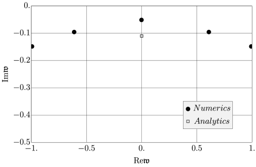
Figure 1: The poles of the scalar channel Green’s function $G_{xy,xy}^{R}(\mathfrak{w},\mathfrak{q})$ in the vicinity of origin in the complex frequency plane at $\mathfrak{q}=0.1$ and $\lambda_{\scriptscriptstyle GB}\approx-7.3125$ (corresponding to $\gamma_{\scriptscriptstyle GB}\approx 5.5$). The poles found numerically are shown by black circles. The white square shows the analytic approximation (71) to the location of the pole on the imaginary axis.

A small frequency expansion of Eq. (2.1) is

$$G_{xy,xy}^{R}(\omega,q)= \,\frac{\sqrt{2}\pi^{4}T^{4}}{\left(1+\gamma_{\scriptscriptstyle GB}\right)^{5/2}\kappa_{5}^{2}}\biggr{[}\gamma_{\scriptscriptstyle GB}+1-2i\mathfrak{w}\gamma_{\scriptscriptstyle GB}^{2}(\gamma_{\scriptscriptstyle GB}+1)\biggr{]}+O(\mathfrak{w}^{2})\,.$$ (72)

A comparison with Eq. (55) gives the familiar expression for pressure (69) and the shear viscosity Brigante:2007nu

$$\eta=\frac{\sqrt{2}\pi^{3}T^{3}L^{3}}{\kappa_{5}^{2}}\frac{\gamma_{\scriptscriptstyle GB}^{2}}{\left(1+\gamma_{\scriptscriptstyle GB}\right)^{3/2}}=\frac{4\pi^{3}T^{3}\tilde{L}^{3}}{\kappa_{5}^{2}}\frac{\gamma_{\scriptscriptstyle GB}^{2}}{\left(1+\gamma_{\scriptscriptstyle GB}\right)^{3}}\,,$$ (73)

where we have reinstated $L$ (or $\tilde{L}$) momentarily. To compute the second-order coefficients $\tau_{\Pi}$ and $\kappa$, we need to include the function $g_{2}$ in the expansion (61) and the solution (56). The resulting expressions for $g_{2}$ and the corresponding Green’s function are very cumbersome and are not shown here explicitly. The small frequency expansion of the Green’s function, however, matches the hydrodynamic result (55) perfectly. Combining the equations (56), (66) and (2.1) and comparing with (55), we can read off the coefficients $\tau_{\Pi}$ and $\kappa$ given by Eqs. (20) and (21), respectively. They coincide with the expressions found earlier in ref. Banerjee:2010zd by using a different method.

The full quasinormal spectrum of metric fluctuations in the scalar channel as a function of $\gamma_{\scriptscriptstyle GB}$ has been analyzed in detail in ref. Grozdanov:2016vgg . The spectrum qualitatively differs from the one at $\lambda_{\scriptscriptstyle GB}=0$ in a number of ways, depending on the sign of $\lambda_{\scriptscriptstyle GB}$. For $\lambda_{\scriptscriptstyle GB}>0$, there is an inflow of new quasinormal frequencies (poles of $G_{xy,xy}^{R}(\omega,q)$ in the complex frequency plane), rising up from complex infinity along the imaginary axis. At the same time, the poles of the two symmetric branches recede from the finite complex plane as $\lambda_{\scriptscriptstyle GB}$ is increased from $0$ to $1/4$, and disappear altogether in the limit $\lambda_{\scriptscriptstyle GB}\rightarrow 1/4$. The spectrum in this limit coincides with the one obtained analytically at $\lambda_{\scriptscriptstyle GB}=1/4$ in section 2.4 of the present paper. For $\lambda_{\scriptscriptstyle GB}<0$, on the contrary, the poles in the symmetric branches become more dense with the magnitude of $\lambda_{\scriptscriptstyle GB}$ increasing, and the two branches gradually lift up towards the real axis. They appear to form branch cuts $(-\infty,-q]\cup[q,\infty)$ in the limit $\gamma_{\scriptscriptstyle GB}\rightarrow\infty$. For small $\mathfrak{q}$ and very large $\gamma_{\scriptscriptstyle GB}$, this would imply accumulation of poles of the Green’s function in the region $|\mathfrak{w}|\ll 1$. We have not investigated this limit in detail. Also, as noted above, there is at least one new pole (seen in Fig. 1) rising up the imaginary axis. The residue and the position of the pole $\mathfrak{w}_{\mathfrak{g}}$ contribute to the shear viscosity and to the position of the corresponding transport peak of the spectral function. A qualitatively similar phenomenon has been observed in the case of ${\cal N}=4$ SYM at large but finite ’t Hooft coupling Grozdanov:2016vgg .

2.2 The shear channel

The energy-momentum tensor two-point functions $G_{zx,zx}$, $G_{tx,tx}$, $G_{tx,zx}$ in the shear channel can be expressed through the single scalar function $G_{2}$ as explained in ref. Kovtun:2005ev . For example,

$$G_{xz,xz}(\omega,q)=\frac{\omega^{2}}{2(\omega^{2}-q^{2})}\,G_{2}(\omega,q)+\cdots,$$ (74)

where the ellipsis represents the contact terms. In holography, the function $G_{2}$ is determined by the solution ${\cal Z}_{2}(u,\omega,q)$ (54) of the equation (47) obeying the appropriate boundary conditions, and by the relevant part of the on-shell boundary action (50).

The retarded correlators in the shear channel are characterized by the presence of the hydrodynamic diffusive mode whose dispersion relation is given by

$$\omega=-i\frac{\eta}{\varepsilon+P}\,q^{2}-i\left[\frac{\eta^{2}\tau_{\Pi}}{(\varepsilon+P)^{2}}-\frac{\theta_{1}}{2(\varepsilon+P)}\right]q^{4}+\cdots,$$ (75)

where $\theta_{1}$ is the transport coefficient of the third-order hydrodynamics introduced in ref.  Grozdanov:2015kqa . Higher terms in the momentum expansion of the shear mode depend on the (unclassified) fourth- and higher-order transport coefficients. Since the Gauss-Bonnet fluid is Weyl-invariant ("conformal"), we have $\varepsilon=3P$ and thus $\eta/(\varepsilon+P)=\left(1-4\lambda_{\scriptscriptstyle GB}\right)/4\pi T=\gamma_{\scriptscriptstyle GB}^{2}/4\pi T$. In holography, the quasinormal mode (75) can be found analytically by solving the equation (47) perturbatively for $\mathfrak{w}\ll 1$, $\mathfrak{q}\ll 1$:

$$\mathfrak{w}= -i\frac{\gamma_{\scriptscriptstyle GB}^{2}}{2}\,\mathfrak{q}^{2}-i\,\frac{\gamma_{\scriptscriptstyle GB}^{4}}{16}\left[(1+\gamma_{\scriptscriptstyle GB})^{2}+2\ln\left(\frac{\gamma_{\scriptscriptstyle GB}}{2(1+\gamma_{\scriptscriptstyle GB})}\right)\right]\,\mathfrak{q}^{4}+\cdots.$$ (76)

The coefficient in front of the term quadratic in momentum coincides with the one predicted by hydrodynamics of the holographic Gauss-Bonnet fluid with known shear viscosity. Since the coefficient $\tau_{\Pi}$ is also known (e.g. from Eq. (55)), the quartic term in (76) allows one to read off the coefficient $\theta_{1}$:

$$\theta_{1}=\frac{\eta}{8\pi^{2}T^{2}}\gamma_{\scriptscriptstyle GB}\left(2\gamma_{\scriptscriptstyle GB}^{2}+\gamma_{\scriptscriptstyle GB}-1\right).$$ (77)

In the dissipationless limit $\gamma_{\scriptscriptstyle GB}\rightarrow 0$ we have $\theta_{1}\sim\gamma_{\scriptscriptstyle GB}^{3}\rightarrow 0$. In fact, it can be seen numerically Grozdanov:2016vgg that the full shear mode (75) approaches zero in the limit $\gamma_{\scriptscriptstyle GB}\rightarrow 0$. At $\gamma_{\scriptscriptstyle GB}=0$ ($\lambda_{\scriptscriptstyle GB}=1/4$), this mode disappears from the spectrum altogether due to the vanishing residue which is consistent with our analytic results for the spectrum at $\lambda_{\scriptscriptstyle GB}=1/4$ in section 2.4.

The full quasinormal spectrum was investigated numerically and partially analytically in ref. Grozdanov:2016vgg . Its behavior as a function of $\lambda_{\scriptscriptstyle GB}$ is qualitatively similar to the one in the scalar channel, with the exception of one curious phenomenon: at fixed $\mathfrak{q}$, the new pole rising up the imaginary axis with (negative) $\lambda_{\scriptscriptstyle GB}$ increasing in magnitude, collides with the hydrodynamic pole (75) at some $\lambda_{\scriptscriptstyle GB}=\lambda_{\scriptscriptstyle GB}^{c}(\mathfrak{q})$, and the two poles move off the imaginary axis. This is interpreted as breakdown of the hydrodynamic regime at a given $\mathfrak{q}=\mathfrak{q}_{c}(\lambda_{\scriptscriptstyle GB})$. Curiously, the range of applicability of the hydrodynamic regime (i.e. the range $\mathfrak{q}\in[0,\mathfrak{q}_{c}])$ increases with the field theory "coupling" (understood as the inverse of $|\lambda_{\scriptscriptstyle GB}|$) increasing Grozdanov:2016vgg .

The retarded correlation functions of the energy-momentum tensor in the shear channel can be computed from the boundary action (50). For the function $G_{2}$ in Eq. (74) we find

$$G_{2}(\omega,q)=4\left(\omega^{2}-q^{2}\right)\frac{\pi^{2}T^{2}}{8\kappa_{5}^{2}}\lim_{\epsilon\rightarrow 0}\mathcal{A}_{2}(\epsilon,\omega,q)\frac{Z_{2}^{\prime}(\epsilon,\omega,q)}{Z_{2}(\epsilon,\omega,q)}\,.$$ (78)

In the hydrodynamic approximation, to first non-trivial order in $\mathfrak{w}$, $\mathfrak{q}$, with both $\mathfrak{w}\sim\mu\ll 1$ and $\mathfrak{q}\sim\mu\ll 1$ scaling the same way, the shear channel solution to Eq. (47) obeying the incoming wave boundary condition is

$$Z_{2}(u)=Z^{(b)}_{2}\left(1-u^{2}\right)^{-i\mathfrak{w}/2}\Biggr{(}1+\frac{i\mathfrak{q}^{2}}{2\mathfrak{w}}\frac{\gamma_{\scriptscriptstyle GB}^{2}}{1-\gamma_{\scriptscriptstyle GB}}\left(1-\sqrt{\gamma_{\scriptscriptstyle GB}^{2}-\gamma_{\scriptscriptstyle GB}^{2}u^{2}+u^{2}}\right)+\frac{i\mathfrak{w}}{4}\Biggl{[}3-\gamma_{\scriptscriptstyle GB}^{2}$$

$$+\left(\gamma_{\scriptscriptstyle GB}^{2}-1\right)u^{2}-2\sqrt{\gamma_{\scriptscriptstyle GB}^{2}-\gamma_{\scriptscriptstyle GB}^{2}u^{2}+u^{2}}+2\ln\frac{1+\sqrt{\gamma_{\scriptscriptstyle GB}^{2}-\gamma_{\scriptscriptstyle GB}^{2}u^{2}+u^{2}}}{2}\Biggr{]}\Biggr{)},$$ (79)

where $Z^{(b)}_{2}$ is the normalization constant. We note that in order to obtain the hydrodynamic dispersion relation (76) that includes information about the second and the third order transport coefficients, we need to find $Z_{2}$ to one order higher, but using the scaling $\omega\sim\mu^{2}$ and $\mathfrak{q}\sim\mu$ is sufficient to extract the diffusive pole.

For the correlation function $G_{2}$ in the regime $\mathfrak{w}\ll 1$, $\mathfrak{q}\ll 1$ we thus find the following expression

$$G_{2}=\frac{2\sqrt{2}\pi^{3}T^{3}\gamma_{\scriptscriptstyle GB}^{2}}{(1+\gamma_{\scriptscriptstyle GB})^{3/2}\kappa_{5}^{2}}\left(\frac{\omega^{2}-q^{2}}{i\omega-i\omega^{2}/\omega_{\mathfrak{g}}-\gamma_{\scriptscriptstyle GB}^{2}q^{2}/4\pi T}\right),$$ (80)

where $\omega_{\mathfrak{g}}=2\pi T\mathfrak{w}_{\mathfrak{g}}$ (see Eq. (71)). At vanishing Gauss-Bonnet coupling $\lambda_{\scriptscriptstyle GB}=0$ ($\gamma_{\scriptscriptstyle GB}=1$) one has $|\mathfrak{w}_{\mathfrak{g}}|\rightarrow\infty$ and we formally recover the standard result for ${\cal N}=4$ SYM at infinitely strong ’t Hooft coupling and infinite $N_{c}$ Policastro:2002se ; Kovtun:2005ev but it should be noted that the formula (80) is accurate only for $|\mathfrak{w}_{\mathfrak{g}}|\ll 1$, i.e. for sufficiently large $\gamma_{\scriptscriptstyle GB}$. The correlator (80) has two poles with the following dispersion relations, expanded to $q^{2}$:

$$\omega_{1} =-i\frac{\gamma_{\scriptscriptstyle GB}^{2}}{4\pi T}q^{2},$$ (81)

$$\omega_{2} =\omega_{\mathfrak{g}}+i\frac{\gamma_{\scriptscriptstyle GB}^{2}}{4\pi T}q^{2}.$$ (82)

The first is the usual diffusive pole, corresponding to quadratic part of the dispersion relation (76), while the second pole is a new non-hydrodynamic pole coming from complex infinity at non-zero $\lambda_{\scriptscriptstyle GB}$. This pole moves up the imaginary axis with $\gamma_{\scriptscriptstyle GB}$ increasing and is responsible for the breakdown of hydrodynamics in the large $\gamma_{\scriptscriptstyle GB}$ limit for any fixed non-zero value of $q$ (see ref. Grozdanov:2016vgg for details).

The above expression for the Green’s function and the dispersion relations are only valid in a (double expansion) regime in which not only $\mathfrak{w}\sim\mathfrak{q}\ll 1$ but also $\gamma_{\scriptscriptstyle GB}\gg 1$. The latter condition is required for the gapped mode on the imaginary axis to satisfy $|\mathfrak{w}|\ll 1$. Note also that the form of the dissipative corrections implies that $\gamma_{\scriptscriptstyle GB}\mathfrak{q}\ll 1$. Obviously, these restrictions are only necessary if we are interested in analytic expressions.

The location of the momentum density diffusion pole confirms the result (11) for the shear viscosity of Gauss-Bonnet holographic fluid. We note that in the limit $\lambda_{\scriptscriptstyle GB}\rightarrow 1/4$ ($\gamma_{\scriptscriptstyle GB}\rightarrow 0$) the residue of the diffusion pole vanishes. The full Green’s function can be determined numerically. The corresponding spectral function in the shear channel for various values of $\gamma_{\scriptscriptstyle GB}$ has been computed numerically in ref. Grozdanov:2016vgg .

2.3 The sound channel

The correlation functions in the sound channel can be expressed through the single scalar function $G_{3}$ Kovtun:2005ev . For example, for the energy density two-point function in the conformal case we have

$$G_{tt,tt}(\omega,q)=-4\frac{\delta^{2}S_{\partial M}}{\delta H_{tt}^{(0)}(\omega,q)\delta H_{tt}^{(0)}(-\omega,-q)}=\frac{2q^{4}}{3(\omega^{2}-q^{2})^{2}}\,G_{3}(\omega,q)+\cdots,$$ (83)

and similar expressions are available for other components of the energy-momentum tensor in the sound channel Policastro:2002tn ; Kovtun:2005ev . To compute $G_{3}$ in holography, one needs the solution ${\cal Z}_{3}(u,\omega,q)$ (54) of the equation (47) and the relevant part of the on-shell boundary action (50). As in Eq. (50), the ellipsis represents the contribution from the contact terms. The function $H_{tt}^{(0)}$ denotes the boundary value of the fluctuation $H_{tt}=h_{tt}/r^{2}=h_{tt}u(1+\gamma_{\scriptscriptstyle GB})/2\pi^{2}T^{2}$.

The hydrodynamic modes in the sound channel are the pair of sound waves whose dispersion relation is predicted by relativistic hydrodynamics up to a quartic term in spatial momentum:

$$\omega=\pm c_{s}\,q-i\Gamma\,q^{2}\mp\frac{\Gamma}{2c_{s}}\left(\Gamma-2c_{s}^{2}\tau_{\Pi}\right)\,q^{3}-i\left[\frac{8\eta^{2}\tau_{\Pi}}{9(\varepsilon+P)^{2}}-\frac{\theta_{1}+\theta_{2}}{3(\varepsilon+P)}\right]\,q^{4}+\cdots\,,$$ (84)

where $c_{s}=1/\sqrt{3}$ is the speed of sound, $\Gamma=2\eta/3(\varepsilon+P)$, $\varepsilon+P=sT$ in the absence of chemical potential, and $\tau_{\Pi}$, $\theta_{1}$, $\theta_{2}$ are transport coefficients of the second- and third-order (conformal) hydrodynamics in four space-time dimensions.

Solving the equation (47) for $Z_{3}$ perturbatively for $\mathfrak{w}\ll 1$, $\mathfrak{q}\ll 1$, imposing the incoming wave boundary condition at the horizon and the Dirichlet condition at the boundary, we find the hydrodynamic quasinormal mode

$$\mathfrak{w}_{1,2}= \pm\frac{1}{\sqrt{3}}\mathfrak{q}-\frac{1}{3}i\gamma_{\scriptscriptstyle GB}^{2}\mathfrak{q}^{2}$$

$$\mp\frac{1}{12\sqrt{3}}\gamma_{\scriptscriptstyle GB}\left(2+\gamma_{\scriptscriptstyle GB}^{3}-6\gamma_{\scriptscriptstyle GB}^{2}-3\gamma_{\scriptscriptstyle GB}+2\gamma_{\scriptscriptstyle GB}\ln\left[\frac{2(1+\gamma_{\scriptscriptstyle GB})}{\gamma_{\scriptscriptstyle GB}}\right]\right)\mathfrak{q}^{3}+\ldots\,.$$ (85)

Comparing the expansion (85) to the prediction (84) of conformal hydrodynamics one finds the same expressions for the shear viscosity - entropy density ratio and the second-order transport coefficient $\tau_{\Pi}$ as the ones reported in Eqs. (19) and (20). This agreement is gratifying but more analytic work is needed to extend the expansion (85) to quartic order and determine the coefficient $\theta_{2}$ of the third-order hydrodynamics. Other features of the quasinormal spectrum are qualitatively similar to the scalar case and are discussed in full detail in ref. Grozdanov:2016vgg .

The coefficients in front of the quadratic, qubic and possibly quartic terms in the dispersion relation (84) vanish in the limit $\gamma_{\scriptscriptstyle GB}\rightarrow 0$. This limit is hard to study numerically but it is conceivable that the higher terms vanish as well leaving the linear propagating mode $\mathfrak{w}=\pm\mathfrak{q}/\sqrt{3}$. Such a mode, however, is absent in the exact spectrum at $\gamma_{\scriptscriptstyle GB}=0$ (see section 2.4).

To first order in the hydrodynamic expansion, the gauge-invariant mode is given by

$$Z_{3}(u)= \,\,Z_{3}^{(b)}\left(1-u^{2}\right)^{-i\mathfrak{w}/2}\Biggr{(}\frac{\gamma_{\scriptscriptstyle GB}^{2}-\sqrt{\gamma_{\scriptscriptstyle GB}^{2}-\gamma_{\scriptscriptstyle GB}^{2}u^{2}+u^{2}}}{(\gamma_{\scriptscriptstyle GB}-1)\gamma_{\scriptscriptstyle GB}^{2}\sqrt{\gamma_{\scriptscriptstyle GB}^{2}-\gamma_{\scriptscriptstyle GB}^{2}u^{2}+u^{2}}}-\frac{3\mathfrak{w}^{2}}{\gamma_{\scriptscriptstyle GB}^{2}\mathfrak{q}^{2}}$$

$$+\frac{i\mathfrak{w}\left(\Xi_{\mathfrak{w}}\mathfrak{w}^{2}+\Xi_{\mathfrak{q}}\mathfrak{q}^{2}\right)}{4\mathfrak{q}^{2}\gamma_{\scriptscriptstyle GB}^{2}\left(1-\gamma_{\scriptscriptstyle GB}^{2}\right)\sqrt{\gamma_{\scriptscriptstyle GB}^{2}-\left(\gamma_{\scriptscriptstyle GB}^{2}-1\right)u^{2}}}\Biggr{)},$$ (86)

where

$$\Xi_{\mathfrak{w}}= -3\left(\gamma_{\scriptscriptstyle GB}^{2}-1\right)U\left(\gamma_{\scriptscriptstyle GB}^{2}-\left(\gamma_{\scriptscriptstyle GB}^{2}-1\right)u^{2}+2U-2\ln(U+1)-3+2\ln 2\right),$$ (87)

$$\Xi_{\mathfrak{q}}= \,\,(\gamma_{\scriptscriptstyle GB}+1)\left(\gamma_{\scriptscriptstyle GB}^{2}\left(9\gamma_{\scriptscriptstyle GB}^{2}-5+2\ln 2\right)+\left(\gamma_{\scriptscriptstyle GB}^{2}-1\right)u^{2}\left(-9\gamma_{\scriptscriptstyle GB}^{2}+U+2\right)\right)$$

$$+(\gamma_{\scriptscriptstyle GB}+1)\left(-U\left(7\gamma_{\scriptscriptstyle GB}^{2}-3+2\ln 2\right)+2\left(U-\gamma_{\scriptscriptstyle GB}^{2}\right)\ln(U+1)\right),$$ (88)

and we have used $U^{2}=u^{2}+\gamma_{\scriptscriptstyle GB}^{2}-u^{2}\gamma_{\scriptscriptstyle GB}^{2}$. The correlation function $G_{3}$ can then be computed from

$$G_{3}(\omega,q)=-\frac{48\left(\omega^{2}-q^{2}\right)^{2}}{\omega^{4}}\frac{\pi^{2}T^{2}}{8\kappa_{5}^{2}}\lim_{\epsilon\rightarrow 0}\mathcal{A}_{3}(\epsilon,\omega,q)\frac{Z_{3}^{\prime}(\epsilon,\omega,q)}{Z_{3}(\epsilon,\omega,q)},$$ (89)

giving

$$G_{3}(\omega,q)=\frac{8\sqrt{2}\pi^{4}T^{4}}{(1+\gamma_{\scriptscriptstyle GB})^{3/2}\kappa_{5}^{2}}\left(\frac{q^{2}-\omega q^{2}/\omega_{\mathfrak{g}}-i\gamma_{\scriptscriptstyle GB}^{2}\omega\left(3\omega^{2}-5q^{2}\right)/4\pi T}{\left(3\omega^{2}-q^{2}\right)\left(1-\omega/\omega_{\mathfrak{g}}\right)+i\gamma_{\scriptscriptstyle GB}^{2}\omega q^{2}/\pi T}\right).$$ (90)

As required by rotational invariance, $G_{1}(\omega,0)=G_{2}(\omega,0)=G_{3}(\omega,0)$ Kovtun:2005ev . The contact term in the on-shell action (50) relevant for the computation of $G_{tt,tt}(\omega,q)$ is

$$S_{\partial M}=\cdots+\frac{\pi^{2}T^{2}}{8\kappa_{5}^{2}}\int\frac{d\omega dq}{(2\pi)^{2}}\,\frac{\sqrt{2}\pi^{2}T^{2}}{3(1+\gamma_{\scriptscriptstyle GB})^{3/2}}\frac{29q^{4}-30\omega^{2}q^{2}+9\omega^{4}}{\left(\omega^{2}-q^{2}\right)^{2}}H^{(0)}_{tt}(-\omega,-q)H^{(0)}_{tt}(\omega,q).$$ (91)

The full retarded energy density two-point function is then

$$G_{tt,tt}(\omega,q)=\frac{3\sqrt{2}\pi^{4}T^{4}}{(1+\gamma_{\scriptscriptstyle GB})^{3/2}\kappa_{5}^{2}}\left(\frac{\left(5q^{2}-3\omega^{2}\right)\left(1-\omega/\omega_{\mathfrak{g}}\right)-i\gamma_{\scriptscriptstyle GB}^{2}\omega q^{2}/\pi T}{\left(3\omega^{2}-q^{2}\right)\left(1-\omega/\omega_{\mathfrak{g}}\right)+i\gamma_{\scriptscriptstyle GB}^{2}\omega q^{2}/\pi T}\right).$$ (92)

The thermodynamic (equilibrium) contribution has been omitted from this expression. To this order in the hydrodynamic expansion, the spectrum contains three modes,

$$\omega_{1,2} =\pm\frac{1}{\sqrt{3}}q-i\frac{\gamma_{\scriptscriptstyle GB}^{2}}{6\pi T}q^{2},$$ (93)

$$\omega_{3} =\omega_{\mathfrak{g}}+i\frac{\gamma_{\scriptscriptstyle GB}^{2}}{3\pi T}q^{2}.$$ (94)

The first two are the attenuated sound modes (85) and the third mode is the gapped mode similar to those in the scalar and shear channels. As in the shear channel, these results require the following scalings to be respected: $\mathfrak{w}\sim\mathfrak{q}\ll 1$, $\gamma_{\scriptscriptstyle GB}\gg 1$ and hence, $\gamma_{\scriptscriptstyle GB}\mathfrak{q}\ll 1$.

Second-order corrections to the two hydrodynamic sound modes were given by Eq. (85). To study the spectrum beyond second-order hydrodynamics and investigate higher-frequency spectrum, we must again resort to numerics. We note that for better control over the numerics, it is useful to follow Kovtun:2006pf and write

$$Z_{3}(u)=\mathcal{A}\left[1+a_{1}u+\cdots\right]+\left(\mathcal{A}\,h\ln u+\mathcal{B}\right)u^{2}\left[1+b_{1}u+\cdots\right],$$ (95)

which is a standard Fröbenius expansion result. The retarded Green’s function is then proportional to $\mathcal{B}/\mathcal{A}$. Because of the logarithmic term in $Z_{3}$, it is beneficial to the precision of our numerics to seek the poles of $\mathcal{B}/\mathcal{A}$ (or zeros of $\mathcal{A}/\mathcal{B}$) as opposed to the zeros of $\mathcal{A}$. Furthermore, the full Green’s function includes information about the values of the residues at the poles. By writing

$$\mathcal{B}=\frac{1}{2}\lim_{u\to 0}\left(Z_{3}^{\prime\prime}(u)-2\mathcal{A}\,h\ln u\right)-\frac{3}{2}\mathcal{A}\,h,$$ (96)

we obtain the following expression convenient for the computation of quasinormal modes:

$$\frac{\mathcal{B}}{\mathcal{A}}=\lim_{u\to 0}\left[\frac{Z_{3}^{\prime\prime}(u)}{2Z_{3}(u)}-h\ln u-\frac{3}{2}h\right].$$ (97)

The coefficient $h$ can be found analytically, $h=-\left(1+\gamma_{\scriptscriptstyle GB}\right)^{4}\left(\mathfrak{w}^{2}-\mathfrak{q}^{2}\right)^{2}/32$. For a detailed discussion of the quasinormal spectrum, see ref. Grozdanov:2016vgg . A comprehensive analysis of the large spatial momentum asymptotics similar to the one accomplished for the strongly coupled ${\cal N}=4$ SYM in refs. Festuccia:2008zx ; Fuini:2016qsc would be of interest but has not been attempted neither in ref. Grozdanov:2016vgg nor in the present paper.

2.4 Exact quasinormal spectrum at $\lambda_{\scriptscriptstyle GB}=1/4$

At $\lambda_{\scriptscriptstyle GB}=1/4$, the equations of motion (47) for all channels simplify drastically. They reduce to the following system

Scalar channel: $$Z_{1}^{\prime\prime}-\frac{2-u}{u(1-u)}Z_{1}^{\prime}+\frac{\mathfrak{w}^{2}-3(1-u)\mathfrak{q}^{2}}{4u(1-u)^{2}}Z_{1}=0,$$ (98)

Shear channel: $$Z_{2}^{\prime\prime}-\frac{2-u}{u(1-u)}Z_{2}^{\prime}+\frac{\mathfrak{w}^{2}}{4u(1-u)^{2}}Z_{2}=0,$$ (99)

Sound channel: $$Z_{3}^{\prime\prime}-\frac{2-u}{u(1-u)}Z_{3}^{\prime}+\frac{\mathfrak{w}^{2}+(1-u)\mathfrak{q}^{2}}{4u(1-u)^{2}}Z_{3}=0.$$ (100)

Solutions to these equations can be written in terms of the hypergeometric function. The indicial exponents of Eqs. (98) - (100) at the horizon at $u=1$ are equal to $\pm i\mathfrak{w}/2$, as expected. Curiously, the exponents at the boundary singular point $u=0$ are $\alpha_{1,2}=\{0,3\}$ and not $\alpha_{1,2}=\{0,2\}$, which are their values for any $\lambda_{\scriptscriptstyle GB}<1/4$ (and in fact for all five-dimensional bulk fluctuations dual to operators of conformal dimension $\Delta=4$ of a $3+1$-dimensional boundary theory). The standard holographic dictionary then implies that at $\lambda_{\scriptscriptstyle GB}=1/4$ the dual theory operators scale as the energy-momentum tensor in six rather than four dimensions. Technically, the reason for this "dimensional transmutation" is related to the fact that the "standard" terms in the wave equations (47) most singular in the limit $u\rightarrow 0$ are multiplied by the coefficients proportional to $(1-4\lambda_{\scriptscriptstyle GB})$ and thus vanish at $\lambda_{\scriptscriptstyle GB}=1/4$. At this value of the Gauss-Bonnet coupling, the theory becomes “topological gravity” Chamseddine:1989nu with a number of curious properties. In particular, thermodynamic properties of the black brane solution at $\lambda_{\scriptscriptstyle GB}=1/4$ are different from the ones at $\lambda_{\scriptscriptstyle GB}<1/4$ Crisostomo:2000bb . The underlying physical reasons and significance of this limit are not entirely clear to us, although they might be related to the issues discussed in ref. Banados:2005rz and refs. Verlinde:1995mz ; Witten:2007ct ; Witten:2009at .

We note that the Gauss-Bonnet black brane metric is regular at $\lambda_{\scriptscriptstyle GB}=1/4$:

$$ds^{2}=-\frac{r^{2}}{L^{2}}\left(1-\frac{r^{2}_{+}}{r^{2}}\right)\,dt^{2}+\frac{L^{2}}{2r^{2}\left(1-\frac{r^{2}_{+}}{r^{2}}\right)}dr^{2}+\frac{r^{2}}{L^{2}}\left(dx^{2}+dy^{2}+dz^{2}\right).$$ (101)

Rescaling the coordinates $t,x,y,z$ and the parameter $L$, it can be brought into the form

$$ds^{2}=-\frac{r^{2}}{L^{2}}\left(1-\frac{r^{2}_{+}}{r^{2}}\right)\,dt^{2}+\frac{L^{2}}{r^{2}\left(1-\frac{r^{2}_{+}}{r^{2}}\right)}dr^{2}+\frac{r^{2}}{L^{2}}\left(dx^{2}+dy^{2}+dz^{2}\right)\,.$$ (102)

For fluctuations depending on $r,t,z$ only, the metric (102) is nothing but the BTZ metric with $T_{L}=T_{R}$ (see e.g. Eq. (4.1) of Son:2002sd with $\rho_{-}=0$) which explains the emergence of the hypergeometric equations in the system of equations (98) - (100). The zero temperature limit of the metric (102) is the standard $AdS_{5}$ solution in Poincaré patch coordinates. Note, however, that the action at $\lambda_{\scriptscriptstyle GB}=1/4$ is obviously not the standard Einstein-Hilbert action, and thus the fluctuation equations are not the "usual" fluctuation equations around $AdS_{5}$ but rather are given by the zero-temperature limit of Eqs. (98) - (100).

The solutions to Eqs. (98) - (100) obeying the incoming wave boundary conditions are given by

Scalar: $$Z_{1}=\left(1-u\right)^{-\frac{i\mathfrak{w}}{2}}{}_{2}F_{1}\left[\Omega-\frac{\sqrt{4-3\mathfrak{q}^{2}}}{2},\Omega+\frac{\sqrt{4-3\mathfrak{q}^{2}}}{2},1-i\mathfrak{w},1-u\right],$$ (103)

Shear: $$Z_{2}=\left(1-u\right)^{-\frac{i\mathfrak{w}}{2}}{}_{2}F_{1}\,\Big{[}\Omega-1,\Omega+1,1-i\mathfrak{w},1-u\Big{]},$$ (104)

Sound: $$Z_{3}=\left(1-u\right)^{-\frac{i\mathfrak{w}}{2}}{}_{2}F_{1}\left[\Omega-\frac{\sqrt{4+\mathfrak{q}^{2}}}{2},\Omega+\frac{\sqrt{4+\mathfrak{q}^{2}}}{2},1-i\mathfrak{w},1-u\right],$$ (105)

where $\Omega\equiv-1-\frac{i\mathfrak{w}}{2}$. Given the three solutions, the quasinormal spectrum is determined analytically by imposing the Dirichlet condition $Z_{i}(0)=0$ at the boundary. We find

Scalar: $$\mathfrak{w}=-i\left(4+2n_{1}-\sqrt{4-3\mathfrak{q}^{2}}\right), \mathfrak{w}=-i\left(4+2n_{2}+\sqrt{4-3\mathfrak{q}^{2}}\right),$$ (106)

Shear: $$\mathfrak{w}=-2i\left(1+n_{1}\right), \mathfrak{w}=-2i\left(3+n_{2}\right),$$ (107)

Sound: $$\mathfrak{w}=-i\left(4+2n_{1}-\sqrt{4+\mathfrak{q}^{2}}\right), \mathfrak{w}=-i\left(4+2n_{2}+\sqrt{4+\mathfrak{q}^{2}}\right),$$ (108)

where $n_{1}$ and $n_{2}$ are independent non-negative integers. The numerical study of the Gauss-Bonnet quasinormal spectrum in ref. Grozdanov:2016vgg shows that in the limit $\lambda_{\scriptscriptstyle GB}\rightarrow 1/4$ the quasinormal frequencies approach the ones found above. The spectrum in the shear channel is $\mathfrak{q}$-independent. In the scalar and sound channels, for sufficintly large $\mathfrak{q}$ the modes cross into the upper half plane of frequency thus signaling an instability. This is perhaps not surprising given the causality problems in the boundary theory observed for sufficiently large spatial momentum in ref. Brigante:2007nu and other publications.

Finally, let us address the questions of what happens to the hydrodynamic poles in the limit of $\lambda_{\scriptscriptstyle GB}\to 1/4$ ($\gamma_{\scriptscriptstyle GB}\to 0$). By examining the limit of the sound correlator $G_{tt,tt}(\omega,q)$ given by Eq. (92) computed for any generic value of $\gamma_{\scriptscriptstyle GB}$ (or the limit of $G_{3}$ given by Eq. (90)), we find a non-vanishing Green’s function with an unattenuated sound mode, $\omega=\pm q/\sqrt{3}$. On the other hand, the sound spectrum computed analytically at $\gamma_{\scriptscriptstyle GB}=0$ (cf. Eq. (108)) contains no such mode. This situation can be contrasted with the shear channel: there, the correlator $G_{2}$ (cf. (80)) vanishes in the same limit and there is no remaining diffusive mode in the spectrum. Consistently, the exact quasinormal spectrum at $\gamma_{\scriptscriptstyle GB}=0$ (cf. (107)) contains no mode at $\mathfrak{w}=0$, either.

We do not have a full understanding of this phenomenon but can offer the following comments. Examine more closely the limit $\gamma_{\scriptscriptstyle GB}\to 0$ of the sound correlator $G_{3}$ (89). First, we notice that its $Z_{3}$-independent prefactor gives different expressions depending on which of the two limits, $\gamma_{\scriptscriptstyle GB}\to 0$ or $\epsilon\to 0$, is taken first. Namely,

$$\lim_{\gamma_{\scriptscriptstyle GB}\to 0}\left[\lim_{\epsilon\to 0}\frac{48\left(\omega^{2}-q^{2}\right)^{2}}{\omega^{4}}\frac{\pi^{2}T^{2}}{8\kappa_{5}^{2}}\mathcal{A}_{3}(\epsilon,\omega,q)\right] =\frac{8\sqrt{2}\pi^{4}T^{4}}{\kappa_{5}^{2}}\frac{\gamma_{\scriptscriptstyle GB}}{\epsilon}+\cdots,$$ (109)

$$\lim_{\epsilon\to 0}\left[\lim_{\gamma_{\scriptscriptstyle GB}\to 0}\frac{48\left(\omega^{2}-q^{2}\right)^{2}}{\omega^{4}}\frac{\pi^{2}T^{2}}{8\kappa_{5}^{2}}\mathcal{A}_{3}(\epsilon,\omega,q)\right] =\frac{72\sqrt{2}\pi^{4}T^{4}}{\kappa_{5}^{2}}\frac{\left(\omega^{2}-q^{2}\right)^{2}}{\left(3\omega^{2}-q^{2}\right)^{2}}\frac{\gamma_{\scriptscriptstyle GB}^{2}}{\epsilon^{2}}+\cdots,$$ (110)

where the ellipses denote terms subleading in the expansions of $\epsilon$ and $\gamma_{\scriptscriptstyle GB}$ around zero. Now, in the expansion around $\gamma_{\scriptscriptstyle GB}=0$, the Fröbenius series (95) becomes

$$Z_{3}(u)=\mathcal{A}+\cdots+\mathcal{B}u^{2}+\left(\frac{\mathcal{A}\left(3\omega^{2}-q^{2}\right)}{144\pi^{2}T^{2}\gamma_{\scriptscriptstyle GB}^{2}}+\cdots-\frac{\mathcal{B}\left(\omega^{2}-q^{2}\right)}{48\pi^{2}T^{2}}\right)u^{3}+\cdots.$$ (111)

By first taking $\epsilon$ and then $\gamma_{\scriptscriptstyle GB}$ to zero (the order of limits we took to find $G_{3}$ in Eq. (90)), one again recovers the leading order hydrodynamic expression

$$G_{3}(\omega,q)=-\frac{16\sqrt{2}\pi^{4}T^{4}\gamma_{\scriptscriptstyle GB}}{\kappa_{5}^{2}}\frac{\mathcal{B}}{\mathcal{A}}=\frac{8\sqrt{2}\pi^{4}T^{4}}{\kappa_{5}^{2}}\frac{q^{2}}{3\omega^{2}-q^{2}}+\cdots.$$ (112)

With the opposite order of limits, the prefactor (110) and the solution (111) yields

$$G_{3}\left(\omega,q\right)=-\frac{3\sqrt{2}\pi^{2}T^{2}}{2\kappa_{5}^{2}}\frac{\left(\omega^{2}-q^{2}\right)^{2}}{\left(3\omega^{2}-q^{2}\right)}\left(1-\frac{\left(\omega^{2}-q^{2}\right)}{\left(\omega^{2}-q^{2}/3\right)}\lim_{\gamma_{\scriptscriptstyle GB}\to 0}\gamma_{\scriptscriptstyle GB}^{2}\frac{\mathcal{B}}{\mathcal{A}}\right),$$ (113)

where $\mathcal{A}$ and $\mathcal{B}$ depend on $\gamma_{\scriptscriptstyle GB}$. What this expression reveals is that it is possible for the unattenuated sound mode to be a pole of the Green’s function, having entered into the expression from the prefactor, not the ratio of $\mathcal{B}/\mathcal{A}$. Thus, such a pole would not appear as a part of the quasinormal spectrum.

2.5 The limit $\lambda_{\scriptscriptstyle GB}\to-\infty$

It is tempting to investigate the limit $\lambda_{\scriptscriptstyle GB}\to-\infty$ analytically to confirm the observations based on numerical simulations. However, taking this limit is problematic for two reasons. First, on a technical level, the equations of motion for fluctuations contain products of the type $\lambda_{\scriptscriptstyle GB}(r-r_{+})$ which remain finite for $r$ sufficiently close to the horizon $r_{+}$, even at large $|\lambda_{\scriptscriptstyle GB}|$. This can possibly be dealt with by a variable redefinition but the second problem is more serious. The Kretschmann curvature invariant evaluated on the black brane solution (29) is

$$R_{\mu\nu\rho\sigma}R^{\mu\nu\rho\sigma}\propto\frac{1}{r^{4}\left(r^{4}\left(1-4\lambda_{\scriptscriptstyle GB}\right)+4r_{+}^{4}\lambda_{\scriptscriptstyle GB}\right)^{3}}.$$ (114)

For $\lambda_{\scriptscriptstyle GB}\in[0,1/4]$, the curvature singularity in Eq. (114) is at $r=0$. However, for $\lambda_{\scriptscriptstyle GB}<0$ the curvature singularity is located at

$$r=\frac{r_{+}}{\left(1-\frac{1}{4\lambda_{\scriptscriptstyle GB}}\right)^{1/4}}.$$ (115)

Thus, as $\lambda_{\scriptscriptstyle GB}$ is tuned from $0$ to $-\infty$, the curvature singularity moves continuously from $r=0$ to the horizon $r=r_{+}$ and becomes a naked singularity in the limit $\lambda_{\scriptscriptstyle GB}\to-\infty$. Because the classical background geometry is singular at the horizon, considering classical metric fluctuations in the limit $\lambda_{\scriptscriptstyle GB}\to-\infty$ would be meaningless. In some sense, the need for an ultraviolet completion of gravity in this limit is in accord with the observations made in ref. Grozdanov:2016vgg and in the present paper that the regime of large negative $\lambda_{\scriptscriptstyle GB}$ qualitatively corresponds to the regime of weak coupling in the field theory which generically requires the full dual stringy rather than dual gravity description.

As a curious observation, we note the following. In the large (negative) $\lambda_{\scriptscriptstyle GB}$ expansion, the Ricci scalar evaluated on the solution (29) to leading order becomes

$$\lim_{\lambda_{\scriptscriptstyle GB}\to-\infty}R=\frac{2\left(15r^{4}r_{+}^{4}-10r^{8}-3r_{+}^{8}\right)}{L^{2}r^{2}\left(r^{4}-r_{+}^{4}\right)^{3/2}}\sqrt{-\frac{1}{\lambda_{\scriptscriptstyle GB}}},$$ (116)

and the leading order contribution to the Kretschmann scalar is

$$\lim_{\lambda_{\scriptscriptstyle GB}\to-\infty}R_{\mu\nu\rho\sigma}R^{\mu\nu\rho\sigma}=\frac{4\left(10r^{16}-30r^{12}r_{+}^{4}+33r^{8}r_{+}^{8}-12r^{4}r_{+}^{12}+3r_{+}^{16}\right)}{L^{4}r^{4}\left(r^{4}-r_{+}^{4}\right)^{3}}\left(\frac{1}{-\lambda_{\scriptscriptstyle GB}}\right).$$ (117)

In fact, all three curvature scalars that appear in the Gauss-Bonnet term, $R_{\mu\nu\rho\sigma}R^{\mu\nu\rho\sigma}$, $R_{\mu\nu}R^{\mu\nu}$ and $R^{2}$, are singular at $r=r_{+}$ and scale as $1/\lambda_{\scriptscriptstyle GB}$, while their combination that appears in the action remains finite and independent of $r$:

$$\lim_{\lambda_{\scriptscriptstyle GB}\to-\infty}\left(R^{2}-4R_{\mu\nu}R^{\mu\nu}+R_{\mu\nu\rho\sigma}R^{\mu\nu\rho\sigma}\right)=-\frac{120}{\lambda_{\scriptscriptstyle GB}L^{4}}.$$ (118)

As as result of these scalings, the Einstein-Gauss-Bonnet action (16) to leading order in $\lambda_{\scriptscriptstyle GB}$ reduces to the Gauss-Bonnet term and the cosmological constant $\Lambda=-6/L^{2}$:

$$\lim_{\lambda_{\scriptscriptstyle GB}\to-\infty}S_{GB}=\frac{\lambda_{\scriptscriptstyle GB}L^{2}}{4\kappa_{5}^{2}}\int d^{5}x\sqrt{-g}\left[R^{2}-4R_{\mu\nu}R^{\mu\nu}+R_{\mu\nu\rho\sigma}R^{\mu\nu\rho\sigma}-\frac{4\Lambda}{\lambda_{\scriptscriptstyle GB}L^{2}}\right].$$ (119)

This theory has a black brane solution that coincides with the $\lambda_{\scriptscriptstyle GB}\to-\infty$ limit of the solution (29),

$$ds^{2}=\sqrt{-\lambda_{\scriptscriptstyle GB}}\left[-\frac{\tilde{r}^{2}}{L^{2}}\sqrt{1-\frac{\tilde{r}_{+}^{4}}{\tilde{r}^{4}}}\,dt^{2}+\frac{L^{2}}{\tilde{r}^{2}\sqrt{1-\frac{\tilde{r}_{+}^{4}}{\tilde{r}^{4}}}}d\tilde{r}^{2}+\frac{\tilde{r}^{2}}{L^{2}}\left(dx^{2}+dy^{2}+dz^{2}\right)\right],$$ (120)

where we have introduced a rescaled radial coordinate $r=\left(-\lambda_{\scriptscriptstyle GB}\right)^{1/4}\tilde{r}$.

3 Gauss-Bonnet transport coefficients from fluid-gravity correspondence

From the analysis of quasinormal spectra and retarded two-point functions in section 2, we were able to determine non-perturbative expressions for the Gauss-Bonnet transport coefficients $\eta$, $\tau_{\Pi}$, $\kappa$ (and also $\theta_{1}$ of the third-order hydrodynamics). To find the remaining transport coefficients, one can use either the fluid-gravity correspondence or the Kubo formulae applied to three-point functions. In this section, we shall use the fluid-gravity methods Bhattacharyya:2008jc ; Rangamani:2009xk . Previously, fluid-gravity approach has been used to determine the shear viscosity Dutta:2008gf and second-order hydrodynamic coefficients Shaverin:2012kv of Gauss-Bonnet holographic liquid perturbatively in $\lambda_{\scriptscriptstyle GB}$.

Fluid-gravity correspondence uses the fact that the bulk metric perturbations $h_{\mu\nu}$ source the energy-momentum tensor $T^{\mu\nu}$ in the generating functional of the boundary quantum field theory Gubser:1998bc ; Witten:1998qj . Gravitational bulk action should thus be able to capture all of the energy-momentum properties of the dual theory. The procedure for computing the holographic energy-momentum tensor, inspired by the old prescription of Brown and York Brown:1992br , was proposed in ref. Balasubramanian:1999re . One expects then that in the appropriate variables a gradient expansion of the bulk metric should capture the hydrodynamic gradient expansion of the dual field theory’s energy-momentum tensor.

Following ref. Bhattacharyya:2008jc , we write the Gauss-Bonnet black brane background solution (29) in the Eddington-Finkelstein coordinates,

$$ds^{2}=-r^{2}f(br)dv^{2}+2N_{\scriptscriptstyle GB}dvdr+r^{2}dx^{i}dx^{i}\,,$$ (121)

where $N_{\scriptscriptstyle GB}$ is given by Eq. (31). We set $L=1$ for convenience and defined $b\equiv 1/r_{+}$ to be consistent with the notations used in ref. Bhattacharyya:2008jc . The function $f(br)$ is

$$f(br)=\frac{N_{\scriptscriptstyle GB}^{2}}{2\lambda_{\scriptscriptstyle GB}}\left[1-\sqrt{1-4\lambda_{\scriptscriptstyle GB}\left(1-\frac{1}{b^{4}r^{4}}\right)}\right].$$ (122)

The energy-momentum tensor is given by the expression

$$T_{\mu\nu}= \,\frac{r^{2}}{\kappa_{5}^{2}}\left[K_{\mu\nu}-K\gamma_{\mu\nu}+\lambda_{\scriptscriptstyle GB}\left(3J_{\mu\nu}-J\gamma_{\mu\nu}\right)+c_{1}\gamma_{\mu\nu}+c_{2}G^{(\gamma)}_{\mu\nu}\right],$$ (123)

where all the ingredients are defined just below Eq. (40).

The next step is to boost the brane solution (121) along a space-time dependent velocity four-vector $u^{a}(x)$, where

$$u^{a}=\frac{1}{\sqrt{1-\beta^{2}}}\left(1,\beta^{i}\right),$$ (124)

with $i=1,2,3$ corresponding to the spatial boundary coordinates. Note that $x^{a}=(v,x,y,z)$ in Eddington - Finkelstein coordinates. The boosted black brane metric, which we denote by $g^{(0)}_{\mu\nu}$, becomes

$$ds_{(0)}^{2}= -2N_{\scriptscriptstyle GB}u_{a}\left(x^{c}\right)dx^{a}dr-r^{2}f\left(b\left(x^{c}\right)r\right)u_{a}\left(x^{c}\right)u_{b}\left(x^{c}\right)dx^{a}dx^{b}$$

$$+r^{2}\Delta_{ab}\left(x^{c}\right)dx^{a}dx^{b}.$$ (125)

Generically, the metric (3) is no longer a solution of the Einstein-Gauss-Bonnet equations of motion (2). In fluid-gravity correspondence, assuming a slow-varying dependence of the coefficients on the coordinates $x^{a}$ and making a gradient expansion, one imposes the equations of motion (2) as the condition each term in the expansion must satisfy. We make a gradient expansions in the derivatives of the fields $\beta^{i}\left(x^{a}\right)$ and $b\left(x^{a}\right)$ to second order, in agreement with the boundary theory’s standard second-order hydrodynamic gradient expansion in velocity and temperature fields (see e.g. Appendix B). To second order, the metric will have the form

$$g_{\mu\nu}=g_{\mu\nu}^{(0)}+\epsilon g^{(1)}_{\mu\nu}+\epsilon^{2}g^{(2)}_{\mu\nu},$$ (126)

where $g_{\mu\nu}^{(0)}$ and $g_{\mu\nu}^{(1)}$ are expanded up to terms involving two derivatives of $b$ and $\beta^{i}$ inclusive. We shall use $\epsilon$ as a book-keeping parameter in the derivative expansion.

The procedure of solving equations (2) order by order is greatly simplified, if one notices that it is sufficient to solve the equations of motion locally around some point $x^{a}=X^{a}$. The global metric can be obtained from these data alone Bhattacharyya:2008jc . The local expansions of the fields $b$ and $\beta^{i}$ are given by

$$b=b_{(0)}|_{X^{a}}+\epsilon x^{a}\partial_{a}b_{(0)}|_{X^{a}}+\epsilon b_{(1)}|_{X^{a}}+\frac{\epsilon^{2}}{2}x^{a}x^{b}\partial_{a}\partial_{b}b_{(0)}|_{X^{a}}+\epsilon^{2}x^{a}\partial_{a}b_{(1)}|_{X^{a}},$$ (127)

$$\beta^{i}=\beta^{i}_{(0)}|_{X^{a}}+\epsilon x^{a}\partial_{a}\beta^{i}_{(0)}|_{X^{a}}+\frac{\epsilon^{2}}{2}x^{a}x^{b}\partial_{a}\partial_{b}\beta^{i}_{(0)}|_{X^{a}}.$$ (128)

We choose to work in a local frame at the origin, $X^{a}=0$, where

$$b_{0}=1 \beta^{i}=0.$$ and (129)

Furthermore, it is consistent to choose a gauge with $\beta^{i}_{(1)}=0$ at $x^{a}=X^{a}$ Bhattacharyya:2008jc .

3.1 First-order solution

The most general expression for the first-order metric $g_{\mu\nu}^{(1)}$ can be conveniently written in a scalar-vector-tensor form

$$ds^{2}_{(1)}=\; \frac{k_{1}(r)}{r^{2}}dv^{2}-3N_{\scriptscriptstyle GB}h_{1}(r)dvdr+\frac{2}{r^{2}}\left(\sum_{i=1}^{3}j_{1}^{i}(r)dx^{i}\right)dv$$

$$+r^{2}h_{2}(r)\left(dx^{2}+dy^{2}+dz^{2}\right)+r^{2}\mathcal{A}_{ab}dx^{a}dx^{b},$$ (130)

where $x^{i}=(x,y,z)$, $k_{1}$ and $h_{1}$ are scalars, $j_{1}^{i}$ is a three-vector and $\mathcal{A}_{ab}$ is a tensor. As discussed above, we proceed by using the expanded forms of $b$ and $\beta^{i}$ given in (127) and (128) to write the order-$\epsilon$ metric as $g_{\mu\nu}=g^{(0)}_{\mu\nu}+\epsilon g^{(1)}_{\mu\nu}$. Then the equations of motion (2) generate the following set of constraints and dynamical equations:

$$\text{Scalar}:\;$$

Constraint 1: $$r^{2}f_{0}(r)E_{vr}+N_{\scriptscriptstyle GB}E_{vv}=0,$$ (131)

Constraint 2: $$r^{2}f_{0}(r)E_{rr}+N_{\scriptscriptstyle GB}E_{vr}=0,$$ (132)

Dynamical equation 1: $$E_{rr}=0,$$ (133)

$$\text{Vector}:\;$$

Constraint 3: $$r^{2}f_{0}(r)E_{ri}+N_{\scriptscriptstyle GB}E_{vi}=0,$$ (134)

Dynamical equation 2: $$E_{ri}=0,$$ (135)

$$\text{Tensor}:\;$$

Dynamical equation 3: $$E_{ij}=0.$$ (136)

First, we solve the Dynamical equation 1 in (133) for $h_{1}(r)$. We then use Constraint 2 in (132) which relates $k_{1}^{\prime}(r)$ to $h_{1}(r)$ to solve for $k_{1}(r)$. Constraints 1 and 3 in (131) and (134) give

$$\partial_{v}b_{0}=\frac{1}{3}\partial_{i}\beta^{i} \partial_{i}b_{0}=\partial_{v}\beta^{i}.$$ and (137)

Finally, we can solve the remaining Dynamical equations 2 and 3 in (135) and (136) to find $j_{1}(r)$ and the tensor $\mathcal{A}_{ab}$ which contains information about shear viscosity.

The global first-order metric, $g_{\mu\nu}=g_{\mu\nu}^{(0)}+\epsilon g_{\mu\nu}^{(1)}$, can be written as a sum Bhattacharyya:2008jc ,

$$ds^{2}=\sum_{n=1}^{6}\mathcal{A}_{n},$$ (138)

where the six line elements $\mathcal{A}_{n}$ are defined as

$$\mathcal{A}_{1}=-2N_{\scriptscriptstyle GB}u_{a}dx^{a}dr, \mathcal{A}_{2}=-r^{2}f_{0}(br)u_{a}u_{b}dx^{a}dx^{b},$$ (139)

$$\mathcal{A}_{3}=r^{2}\Delta_{ab}dx^{a}dx^{b}, \mathcal{A}_{4}=2r^{2}bF_{0}(br)\sigma_{ab}dx^{a}dx^{b},$$ (140)

$$\mathcal{A}_{5}=\frac{2}{3}N_{\scriptscriptstyle GB}ru_{a}u_{b}\partial_{c}u^{c}dx^{a}dx^{b}, \mathcal{A}_{6}=-N_{\scriptscriptstyle GB}ru^{c}\partial_{c}\left(u_{a}u_{b}\right)dx^{a}dx^{b}.$$ (141)

The last step is to find the function $F_{0}(r)$ entering Eq. (140). This function is part of the tensor $\mathcal{A}_{ab}$ satisfying Eq. (136). Explicitly, the second-order differential equation for $F_{0}$ is

$$\frac{\partial}{\partial r}\left[\left(r^{5}-\frac{r^{7}}{\sqrt{1-\left(1-r^{4}\right)\gamma_{\scriptscriptstyle GB}^{2}}}\right)\frac{\partial F_{0}}{\partial r}\right]=\frac{\left(1-\gamma_{\scriptscriptstyle GB}^{2}\right)\left(5-\left(5-3r^{4}\right)\gamma_{\scriptscriptstyle GB}^{2}\right)r^{4}}{2\sqrt{2}\sqrt{1+\gamma_{\scriptscriptstyle GB}}\left(1-\left(1-r^{4}\right)\gamma_{\scriptscriptstyle GB}^{2}\right)^{3/2}}.$$ (142)

A pleasant feature of fluid-gravity duality is that the kernel (the part involving the derivatives) of dynamical equations remains the same for all unknown functions at all orders in the gradient expansion. This was manifest in Eq. (62) and we expect the same from the equations such as Eq. (142). A solution to Eq. (142) regular at the horizon and vanishing at the boundary is given by

$$F_{0}(r)= ~{}\frac{1}{8\sqrt{2}}\Biggr{\{}\frac{(1+i)\left(1-\gamma_{\scriptscriptstyle GB}^{2}\right)^{1/4}\left[(1-i)\;\text{arctanh}(\gamma_{\scriptscriptstyle GB})+\pi-(1-i)\gamma_{\scriptscriptstyle GB}\right]}{(1-\gamma_{\scriptscriptstyle GB})^{1/4}(1+\gamma_{\scriptscriptstyle GB})^{3/4}}$$

$$+\frac{\gamma_{\scriptscriptstyle GB}^{3/2}\Gamma\left(\frac{1}{4}\right)^{2}\,_{2}F_{1}\left[\frac{1}{4},1;\frac{1}{2};\frac{1}{1-\gamma_{\scriptscriptstyle GB}^{2}}\right]}{\sqrt{\pi}(1-\gamma_{\scriptscriptstyle GB})^{1/4}(1+\gamma_{\scriptscriptstyle GB})^{3/4}}+\frac{1-\gamma_{\scriptscriptstyle GB}^{2}-i\pi r^{4}+2r^{2}\sqrt{1-\left(1-r^{4}\right)\gamma_{\scriptscriptstyle GB}^{2}}}{\sqrt{\gamma_{\scriptscriptstyle GB}}r^{4}}$$

$$+\frac{1}{\sqrt{1+\gamma_{\scriptscriptstyle GB}}}\ln\left[\frac{(1+r)^{2}\left(1+r^{2}\right)\left(r^{2}-\sqrt{1-\left(1-r^{4}\right)\gamma_{\scriptscriptstyle GB}^{2}}\right)}{r^{4}\left(r^{2}+\sqrt{1-\left(1-r^{4}\right)\gamma_{\scriptscriptstyle GB}^{2}}\right)}\right]$$

$$-\frac{2}{\sqrt{1+\gamma_{\scriptscriptstyle GB}}}\;\text{arctan}(r)+\frac{4r\sqrt{1-\gamma_{\scriptscriptstyle GB}^{2}}}{\sqrt{1+\gamma_{\scriptscriptstyle GB}}}F_{1}\left[\frac{1}{4},-\frac{1}{2},1;\frac{5}{4};-\frac{\gamma_{\scriptscriptstyle GB}^{2}r^{4}}{1-\gamma_{\scriptscriptstyle GB}^{2}},r^{4}\right]\Biggr{\}},$$ (143)

where $F_{1}(a,b,b^{\prime};c;w,z)$ is the Appell hypergeometric function of two variables and where ${}_{2}F_{1}(a,b;c;z)$ is the Gauss hypergeometric function. The expansion of the Appell function at $r\rightarrow\infty$ (explicitly written here for $0<\gamma_{\scriptscriptstyle GB}<1$) can be found by using the theorems in ref. ferreira2004asymptotic :

$$F_{1}\left[\frac{1}{4},-\frac{1}{2},1;\frac{5}{4};-\frac{\gamma_{\scriptscriptstyle GB}^{2}r^{4}}{1-\gamma_{\scriptscriptstyle GB}^{2}},r^{4}\right]=-\frac{\Gamma\left(\frac{1}{4}\right)\Gamma\left(\frac{5}{4}\right)\,_{2}F_{1}\left[\frac{1}{4},1;\frac{1}{2};\frac{1}{1-\gamma_{\scriptscriptstyle GB}^{2}}\right]}{\sqrt{\pi}}\left(\frac{\gamma_{\scriptscriptstyle GB}^{2}}{1-\gamma_{\scriptscriptstyle GB}^{2}}\right)^{3/4}\frac{1}{r}$$

$$+\left(\frac{\gamma_{\scriptscriptstyle GB}^{2}}{1-\gamma_{\scriptscriptstyle GB}^{2}}\right)^{1/2}\frac{1}{r^{2}}+\frac{27\left(8-\gamma_{\scriptscriptstyle GB}^{2}\right)\Gamma\left(-\frac{3}{4}\right)^{3}}{2048\sqrt{\pi}\gamma_{\scriptscriptstyle GB}^{5/2}\left(1-\gamma_{\scriptscriptstyle GB}^{2}\right)^{7/4}\Gamma\left(\frac{1}{4}\right)}$$

$$\times\left\{\left(1-\gamma_{\scriptscriptstyle GB}^{2}\right)\left(\,{}_{2}F_{1}\left[-\frac{3}{4},1;\frac{1}{2};\frac{1}{1-\gamma_{\scriptscriptstyle GB}^{2}}\right]+2\right)+3\gamma_{\scriptscriptstyle GB}^{2}\,{}_{2}F_{1}\left[\frac{1}{4},1;\frac{1}{2};\frac{1}{1-\gamma_{\scriptscriptstyle GB}^{2}}\right]\right\}\frac{1}{r^{5}}+\cdots.$$ (144)

The result (3.1) allows us to find the expansion of $F_{0}(r)$ near the boundary,

$$F_{0}(r)=\frac{\sqrt{1+\gamma_{\scriptscriptstyle GB}}}{2\sqrt{2}r}-\frac{\gamma_{\scriptscriptstyle GB}\sqrt{1+\gamma_{\scriptscriptstyle GB}}}{8\sqrt{2}r^{4}}+\mathcal{O}\left(r^{-5}\right),$$ (145)

valid to order $\mathcal{O}(r^{-4})$ which is sufficient for the purposes of computing the boundary energy-momentum tensor. Substituting $F_{0}(r)$ into the first-order metric $g^{\mu\nu}_{(1)}$ and computing the energy-momentum tensor (123) with the full first-order solution we recover the non-perturbative result for the shear viscosity $\eta$ presented in (73).

3.2 Second-order solution

The second-order correction $g^{(2)}_{\mu\nu}$ is computed in a similar way: first, we perturb $g^{(0)}_{\mu\nu}+\epsilon g^{(1)}_{\mu\nu}$ to second order in derivative expansion and then find $g^{(2)}_{\mu\nu}$ requiring that the Einstein-Gauss-Bonnet equations of motion (2) are satisfied.

To find the second-order transport coefficients non-perturbatively, we would need to solve differential equations with the differential operator given by the left-hand side of Eq. (142) and the right-hand sides involving integrals over the Appell function (3.1). This program faces a certain technical challenge, and we were not able to find closed-form expressions for the transport coefficients in this way. It is possible, however, to obtain terms of the perturbative expansion of transport coefficients in $\gamma_{\scriptscriptstyle GB}$ and thus check the fully non-perturbative results (20), (22), (23) found by using the method of three-point functions (see ref. Grozdanov:2015asa and section 4), as well as perturbative results by Shaverin Shaverin:2012kv .

A convenient ansatz for the line element of the second-order metric $g_{\mu\nu}^{(2)}$ is suggested by the tensor structure of second-order hydrodynamics (see e.g. Appendix B):

$$ds^{2}_{(2)}=\; \frac{k_{2}(r)}{r^{2}}dv^{2}-3N_{\scriptscriptstyle GB}h_{2}(r)dvdr+\frac{2}{r^{2}}\left(\sum_{i=1}^{3}j_{2}^{i}(r)dx^{i}\right)dv$$

$$+r^{2}h_{2}(r)\left(dx^{2}+dy^{2}+dz^{2}\right)+r^{2}\sum_{n=0}^{3}P_{n}(r)\mathcal{B}_{n},$$ (146)

where $x^{i}=(x,y,z)$, $k_{2}$ and $h_{2}$ are scalars, $j_{2}^{i}$ is a three-vector. We have also defined

$$\mathcal{B}_{0}=\left({}_{\langle}D\sigma_{ab\rangle}+\frac{1}{3}\sigma_{ab}\left(\nabla\cdot u\right)\right)dx^{a}dx^{b},$$ (147)

$$\mathcal{B}_{1}=\sigma_{\langle a}^{~{}~{}c}\sigma_{b\rangle c}\;dx^{a}dx^{b},$$ (148)

$$\mathcal{B}_{2}=\sigma_{\langle a}^{~{}~{}c}\Omega_{b\rangle c}\;dx^{a}dx^{b},$$ (149)

$$\mathcal{B}_{3}=\Omega_{\langle a}^{~{}~{}c}\Omega_{b\rangle c}\;dx^{a}dx^{b}.$$ (150)

At this point, we can focus only on the four functions $P_{n}$, $n=\{0,1,2,3\}$, which will give us the four second-order coefficients, $\lambda_{0}\equiv\eta\tau_{\Pi}$, $\lambda_{1}$, $\lambda_{2}$ and $\lambda_{3}$, respectively. Since the boundary theory is defined in flat space-time, this procedure will not allow us to find the coefficient $\kappa$. Furthermore, we know that in Landau frame there are no other transport coefficients coming from either the scalar or the vector sector. Still, we need to use the constraint equation $r^{2}f_{0}(r)E_{rr}+N_{\scriptscriptstyle GB}E_{vr}=0$ and the dynamical equation $E_{rr}=0$ to eliminate $h_{2}$, $k_{2}$ and their derivatives from the dynamical equations for $P_{n}$.

The remaining differential equations for $P_{n}$ can be solved perturbatively to an arbitrarily high order in $\lambda_{\scriptscriptstyle GB}$. Here we outline what we believe is the most efficient way to extract information from the functions $P_{n}$ necessary to recover the four transport coefficients $\lambda_{0,1,2,3}$. First, the functions $P_{n}$ are expanded in series near the boundary as

$$P_{n}(r)=\sum_{i=1}^{\infty}\frac{p^{(i)}_{n}}{r^{i}}.$$ (151)

Then the metric (3.2) with $P_{n}$ expanded as in Eq. (151) is substituted into the full second-order metric, and the energy-momentum tensor (123) is computed. The main observation is that in the limit $r\to\infty$, finite contributions to $T_{\mu\nu}$ only depend on the coefficients of $P_{n}$ proportional to $r^{-4}$, i.e. $T_{\mu\nu}$ depends on $p_{1}^{(4)}$, $p_{2}^{(4)}$, $p_{3}^{(4)}$ and $p_{4}^{(4)}$.

In order to find the four coefficients, we use the fact that all four differential equations for $P_{n}(r)$ can be written in the form of Eq. (142), i.e. as

$$\partial_{r}\left[Q(r)\partial_{r}P_{n}(r)\right]-R_{n}(r)=0,$$ (152)

where $Q$ and $R$ expanded to the desired order in $\lambda_{\scriptscriptstyle GB}$, and the function $Q$ is the same in all four cases. The differential equations can be formally solved, as in Eq. (64), by writing

$$P_{n}(r)=D_{n}+\int^{r}dr^{\prime}\frac{1}{Q(r^{\prime})}\left(C_{n}-\int^{r^{\prime}}dr^{\prime\prime}R_{n}(r^{\prime\prime})\right).$$ (153)

Fortunately, in Eq. (153) it is sufficient to take the inner integral over $r^{\prime\prime}$ whose integrand depends on $F_{0}(r)$ expanded to the desired order of $\lambda_{\scriptscriptstyle GB}$. Integration constants $C_{n}$ are fixed by requiring regularity at the horizon. The coefficients $D_{n}$ may remain undetermined since we only need the specific terms in the $r\to\infty$ expansion. Thus, using the expansion (151) in the differential equations (153) we find all $p^{(4)}_{n}$. For example, from the equation obeyed by $P_{0}$ we obtain

$$\frac{p^{(1)}_{0}}{r^{2}}+\frac{2p^{(2)}_{0}}{r^{3}}+\frac{3p^{(3)}_{0}}{r^{4}}+\frac{1}{r^{5}}\left[4p^{(4)}_{0}+\left(-1+\frac{\ln 2}{2}\right)\right.$$

$$\left.+\left(\frac{19}{4}-\ln 2\right)\lambda_{\scriptscriptstyle GB}+\left(\frac{1}{8}-\ln 2\right)\lambda_{\scriptscriptstyle GB}^{2}+\ldots\right]+\mathcal{O}\left(r^{-6}\right)=0$$ (154)

which allows us to find $p^{(4)}_{0}$ to the desired order in $\lambda_{\scriptscriptstyle GB}$ by setting to zero the coefficient in front of $r^{-5}$.

3.3 Transport coefficients

Once the coefficients $p^{(4)}_{n}$ are known, the full second-order metric can be used to determine the expansion of the energy-momentum tensor (123) near $r\to\infty$ and read off the transport coefficients $\eta\tau_{\Pi}$, $\lambda_{1}$, $\lambda_{2}$ and $\lambda_{3}$ from the coefficients of tensors (147) - (150). The results are in exact agreement with the corresponding terms of the $\lambda_{\scriptscriptstyle GB}$-expansions of the four non-perturbative second-order transport coefficients given by Eqs. (20), (22), (23) and (24), as well as with those computed in ref. Shaverin:2012kv to linear order.

The conclusion of this section is that fluid-gravity duality applied to Gauss-Bonnet holographic fluid allows to determine all the transport coefficients of second-order hydrodynamics, except $\kappa$, but only the shear viscosity $\eta$ is determined non-perturbatively in $\lambda_{\scriptscriptstyle GB}$: the coefficients $\tau_{\Pi}$ and $\lambda_{1,2,3}$ are found only as series in $\lambda_{\scriptscriptstyle GB}$, due to technical problems related to evaluating integrals of Appell function. Finally, we note that within the fluid-gravity approach one is able to check the Haack-Yarom relation order by order in $\lambda_{\scriptscriptstyle GB}$ and find that it is violated at quadratic order as shown in Eq. (26).

4 Gauss-Bonnet transport from three-point functions

The full non-perturbative expressions for the Gauss-Bonnet transport coefficients can be found by computing the three-point functions of the energy-momentum tensor in the hydrodynamic approximation and using the Kubo-type formulae derived in refs. Moore:2010bu ; Saremi:2011nh ; Arnold:2011ja . The retarded three-point functions are defined following the recipes of the Schwinger-Keldysh closed time-path formalism Schwinger:1960qe ; Keldysh:1964ud . Part of the material in this section has some overlap with refs. Grozdanov:2014kva ; Grozdanov:2015asa and is included here for convenience and continuity.

4.1 An overview of the method

In the Schwinger-Keldysh formalism, given a Lagrangian $\mathcal{L}\left[\phi,h\right]$, where $\phi$ collectively denotes matter fields and $h$ is a metric perturbation around a fixed background $g$, the degrees of freedom are doubled: $\phi\to\phi^{\pm}$, $g\to g^{\pm}$, $h\to h^{\pm}$, where the index $\pm$ labels the fields defined either on a “$+$"-time contour running from $t_{0}$ towards the final time $t_{f}>t_{0}$ or the “$-$"-time contour, where the time runs from $t_{f}$ backwards to $t_{0}$. When the theory is considered at finite temperature $T=1/\beta$, the two real-time contours can be joined by a third, imaginary time, contour running between $t_{f}$ and $t_{f}-i\beta$. Fields defined on this imaginary time contour will be denoted by $\varphi$. The generating functional of the energy-momentum tensor correlation functions is given by

$$W\left[h^{+},h^{-}\right]= \ln\int\mathcal{D}\phi^{+}\mathcal{D}\phi^{-}\mathcal{D}\varphi\exp\left\{i\int d^{4}x^{+}\sqrt{-g^{+}}\mathcal{L}\left[\phi^{+}(x^{+}),h^{+}\right]\right.$$

$$\left.-\int_{0}^{\beta}d^{4}y\mathcal{L}_{E}\left[\varphi(y)\right]-i\int d^{4}x^{-}\sqrt{-g^{-}}\mathcal{L}\left[\phi^{-}(x^{-}),h^{-}\right]\right\}.$$ (155)

For all fields, it will be convenient to use Keldysh basis $\phi_{R}=\frac{1}{2}\left(\phi^{+}+\phi^{-}\right)$ and $\phi_{A}=\phi^{+}-\phi^{-}$. Upon computing the variation, classical expectation values obey $\phi^{+}=\phi^{-}$. Thus, all fields with an index $A$ will vanish and one can define $T^{ab}\equiv T^{ab}_{R}$:

$$\left\langle T^{ab}_{R}(x)\right\rangle=-\frac{2i}{\sqrt{-g}}\frac{\partial W}{\partial h_{A\;ab}(x)}\biggr{|}_{h=0}.$$ (156)

The expectation value of $T_{R}$ at $x=0$ can be expanded as

$$\left\langle T^{ab}_{R}(0)\right\rangle= \,\,G^{ab}_{R}(0)-\frac{1}{2}\int d^{4}x\,G^{ab,cd}_{RA}(0,x)h_{cd}(x)$$

$$+\frac{1}{8}\int d^{4}xd^{4}y\,G^{ab,cd,ef}_{RAA}(0,x,y)h_{cd}(x)h_{ef}(y)+\ldots,$$ (157)

where $G_{RAA...}$ denote the fully retarded Green’s functions Wang:1998wg obtained by

$$G^{ab,cd,\ldots}_{RA\ldots}(0,x,\ldots)=\frac{(-i)^{n-1}(-2i)^{n}\partial^{n}W}{\partial h_{A\;ab}(0)\partial h_{R\;cd}(x)\ldots}\biggr{|}_{h=0}=(-i)^{n-1}\left\langle T_{R}^{ab}(0)T_{A}^{cd}(x)\ldots\right\rangle,$$ (158)

where the ellipses indicate further insertions of $\partial h_{R}$ in the expression with the derivatives as well as the $T_{A}^{ab}$ insertions into the n-point function on the right-hand side of Eq. (158).

We follow refs. Moore:2010bu ; Saremi:2011nh and use Kubo formulae for pressure and transport coefficients of a conformal fluid derived by exciting fluctuations of the relevant metric components. Choosing the spatial momentum along the $z$ direction, one turns on $h_{xy}$, $h_{xz}$ and $h_{yz}$ perturbations to obtain

$$\eta=i\lim_{p,q\to 0}\frac{\partial}{\partial q^{0}}G^{xy,xz,yz}_{RAA}(p,q),$$ (159)

$$2\eta\tau_{\Pi}-\kappa=\lim_{p,q\to 0}\frac{\partial^{2}}{\partial\left(p^{0}\right)^{2}}G^{xy,xz,yz}_{RAA}(p,q),$$ (160)

$$\lambda_{1}=\eta\tau_{\Pi}-\lim_{p,q\to 0}\frac{\partial^{2}}{\partial p^{0}\partial q^{0}}G^{xy,xz,yz}_{RAA}(p,q).$$ (161)

By turning on $h_{xy}$, $h_{tx}$ and $h_{ty}$ components, we find

$$\lambda_{3}=4\lim_{p,q\to 0}\frac{\partial^{2}}{\partial p^{z}\partial q^{z}}G^{xy,tx,ty}_{RAA}(p,q),$$ (162)

$$\kappa=\lim_{p,q\to 0}\frac{\partial^{2}}{\partial\left(p^{z}\right)^{2}}G^{xy,tx,ty}_{RAA}(p,q),$$ (163)

and, finally, by considering $h_{xy}$, $h_{ty}$ and $h_{xz}$ perturbations, we obtain

$$\lambda_{2}=2\eta\tau_{\Pi}-4\lim_{p,q\to 0}\frac{\partial^{2}}{\partial p^{0}\partial q^{z}}G^{xy,ty,xz}_{RAA}(p,q).$$ (164)

A consistency check on our calculations is provided by the following two Kubo formulae which both give the expression for pressure:

$$P=\lim_{p^{0}\to 0}\lim_{q^{0}\to 0}G^{xy,xz,yz}_{RAA}(p,q)=-\lim_{p^{z}\to 0}\lim_{q^{z}\to 0}G^{xy,tx,ty}_{RAA}(p,q).$$ (165)

Note that our definitions of transport coefficients are the same as in ref. Baier:2007ix (see Appendix B for a digest of notations and conventions used in the literature).

4.2 The three-point functions in the hydrodynamic limit

The three-point functions are computed by solving the Einstein-Gauss-Bonnet equations of motion (2) to second order in relevant perturbations,

$$g_{\mu\nu}\rightarrow g_{\mu\nu}+\epsilon r^{2}h^{(1)}_{\mu\nu}+\epsilon^{2}r^{2}h^{(2)}_{\mu\nu},$$ (166)

where the book-keeping parameter $\epsilon$ is used to indicate the order of perturbation. The Dirichlet condition $h^{(2)}_{\mu\nu}=0$ is imposed at the boundary Saremi:2011nh . Once the bulk solutions are found, one should take the triple variation of the on-shell action with respect to the boundary values $h^{(b)}_{\mu\nu}=h^{(1)}_{\mu\nu}\left(r\to\infty\right)$ to find the correlators. A simplifying feature of this procedure is that since equations of motion are solved to order $\epsilon^{2}$, only the boundary term contributes to the three-point function, and hence no bulk-to-bulk propagators appear in the calculation.

To compute the three-point functions used in the Kubo formulae above, we need to turn on the following sets of metric perturbations:

$$1) h_{xy}=h_{xy}(r)e^{-i\left(p^{0}+q^{0}\right)t}, h_{xz}=h_{xz}(r)e^{-ip^{0}t}, h_{yz}=h_{yz}(r)e^{-iq^{0}t},$$ (167)

$$2) h_{xy}=h_{xy}(r)e^{i\left(p^{z}+q^{z}\right)z}, h_{tx}=h_{tx}(r)e^{ip^{z}z}, h_{ty}=h_{ty}(r)e^{iq^{z}z},$$ (168)

$$3) h_{xy}=h_{xy}(r)e^{-ip^{0}t+iq^{z}z}, h_{xz}=h_{xz}(r)e^{-ip^{0}t}, h_{ty}=h_{ty}(r)e^{iq^{z}z}.$$ (169)

Here, we outline the steps leading to obtaining the three-point function $G^{xy,xz,yz}_{RAA}$. First, we find the bulk solutions for $h_{xy}^{(1)}$, $h_{xz}^{(1)}$ and $h_{yz}^{(1)}$ imposing the standard incoming wave boundary condition at the horizon and the condition $h^{(1)}_{\mu\nu}=h^{(b)}_{\mu\nu}$ at the boundary. As in section 2.1, it will be convenient to work with the radial variable $v$ defined by Eq. (48).

Since the metric fluctuations in the set (167) are independent of the spatial momentum, all three of them obey the same differential equation (47), and thus $h_{xy}^{(1)}$, $h_{xz}^{(1)}$ and $h_{yz}^{(1)}$ will have the same functional dependence on $v$. Moreover, we can use the solution to the equation already obtained in section 2.1, with $\mathfrak{q}$ set to zero and the relevant frequencies, $p^{0}+q^{0}$, $p^{0}$ and $q^{0}$, inserted instead of $\mathfrak{w}$, respectively. Thus, for $h_{xy}^{(1)}$ we find the expression

$$h_{xy}^{(1)}(v)=h^{(b)}_{xy}\,\left(\frac{v}{2\lambda_{\scriptscriptstyle GB}}\right)^{-\frac{i(p^{0}+q^{0})}{4\pi T}}\Biggr{[}1+\frac{i(p^{0}+q^{0})}{8\pi T}\left(4-v\right)v+\frac{(p^{0}+q^{0})^{2}}{4\pi^{2}T^{2}}g^{(\mathfrak{w})}_{2}(v)$$

$$+\frac{(p^{0}+q^{0})^{2}}{16\pi^{2}T^{2}}\int^{v}\frac{(1-v^{\prime})^{2}\ln\left[\gamma_{\scriptscriptstyle GB}^{2}-1+v^{\prime}-\sqrt{\left(\gamma_{\scriptscriptstyle GB}^{2}-1\right)\left(\gamma_{\scriptscriptstyle GB}^{2}-(1-v^{\prime})^{2}\right)}\right]}{v^{\prime}}\,dv^{\prime}\Biggr{]},$$ (170)

and similar formulas for $h_{xz}^{(1)}$ and $h_{yz}^{(1)}$. We can deal with the remaining integral in Eq. (4.2) in the same way as in section 2.1, by integrating order-by-order in the near-boundary expansion.

Next, we need to look for the second-order solution $h^{(2)}_{xy}$, which includes the first-order metric back-reaction. The differential equation again has the form of Eq. (62) and can be solved using the same methods. The relevant part of the solution takes the following form:

$$h^{(2)}_{xy}=h^{(b)}_{xz}h^{(b)}_{yz}\,\left(\frac{v}{2\lambda_{\scriptscriptstyle GB}}\right)^{-i(p^{0}+q^{0})/(4\pi T)}\,\frac{p^{0}q^{0}}{4\pi^{2}T^{2}}h(v),$$ (171)

with a complicated and unilluminating expression for $h(v)$ not shown here explicitly.

With the second-order solution in hand, we substitute the resulting formula for $g_{\mu\nu}+\epsilon r^{2}h^{(1)}_{\mu\nu}+\epsilon^{2}r^{2}h^{(2)}_{\mu\nu}$ into the expression for the holographic energy-momentum tensor (123) to compute $T^{xy}$. Finally, taking derivatives with respect to $h^{(b)}_{xz}$ and $h^{(b)}_{yz}$, we obtain $G^{xy,xz,yz}_{RAA}$:

$$G^{xy,xz,yz}_{RAA}(p,q)=\frac{\sqrt{2}\pi^{4}T^{4}}{\left(1+\gamma_{\scriptscriptstyle GB}\right)^{3/2}\kappa_{5}^{2}}-i\left(p^{0}+q^{0}\right)\frac{\sqrt{2}\pi^{3}T^{3}}{\kappa_{5}^{2}}\frac{\gamma_{\scriptscriptstyle GB}^{2}}{\left(1+\gamma_{\scriptscriptstyle GB}\right)^{3/2}}$$

$$+\frac{(p^{0})^{2}+(q^{0})^{2}}{2}\left[\frac{\pi^{2}T^{2}}{2\sqrt{2}\kappa_{5}^{2}}\frac{(\gamma_{\scriptscriptstyle GB}+1)\left(\gamma_{\scriptscriptstyle GB}\left(\gamma_{\scriptscriptstyle GB}^{2}+\gamma_{\scriptscriptstyle GB}-2\right)+2\right)+2\gamma_{\scriptscriptstyle GB}^{2}\ln\left[\frac{\gamma_{\scriptscriptstyle GB}}{2(1+\gamma_{\scriptscriptstyle GB})}\right]}{(1+\gamma_{\scriptscriptstyle GB})^{3/2}}\right]$$

$$+p^{0}q^{0}\left[\frac{\pi^{2}T^{2}}{4\sqrt{2}\kappa_{5}^{2}}\frac{\left(-3\gamma_{\scriptscriptstyle GB}^{2}+2\gamma_{\scriptscriptstyle GB}+11\right)\gamma_{\scriptscriptstyle GB}^{2}-6+2\gamma_{\scriptscriptstyle GB}^{2}\ln\left[\frac{\gamma_{\scriptscriptstyle GB}}{2(1+\gamma_{\scriptscriptstyle GB})}\right]}{(1+\gamma_{\scriptscriptstyle GB})^{3/2}}\right].$$ (172)

The other three-point functions, $G^{xy,tx,ty}_{RAA}$ and $G^{xy,ty,xz}_{RAA}$, are computed using the same procedure, with the differential equations always taking the form of (47). The only difference is that we cannot impose the in-falling boundary conditions on perturbations $h_{tx}$ or $h_{ty}$ in Eq. (168), and similarly on $h_{ty}$ in Eq. (169), because they only fluctuate in the $z$-direction and not time. Regularity then demands setting $h_{tx}=h_{ty}=0$ at the horizon. Consequently, $h_{xy}$ in Eq. (168) also needs to vanish at the horizon.

4.3 Second-order transport coefficients and the zero-viscosity limit

Having computed in the hydrodynamic approximation the three-point functions $G^{xy,xz,yz}_{RAA}$, $G^{xy,tx,ty}_{RAA}$ and $G^{xy,ty,xz}_{RAA}$, we can use the Kubo formulae to compute pressure (165), shear viscosity (159) and all second-order transport coefficients (160) – (164). The result for pressure coincides with the one in Eq. (69), and the shear viscosity is confirmed to be given by Eq. (73). For the second-order transport coefficients we find $(L=1)$:

$$\eta\tau_{\Pi}=\frac{\pi^{2}T^{2}}{4\sqrt{2}\kappa_{5}^{2}}\frac{\gamma_{\scriptscriptstyle GB}}{\left(1+\gamma_{\scriptscriptstyle GB}\right)^{\frac{3}{2}}}\Biggl{[}\left(1+\gamma_{\scriptscriptstyle GB}\right)\left(5\gamma_{\scriptscriptstyle GB}+\gamma_{\scriptscriptstyle GB}^{2}-2\right)-2\gamma_{\scriptscriptstyle GB}\ln\left(\frac{2\left(1+\gamma_{\scriptscriptstyle GB}\right)}{\gamma_{\scriptscriptstyle GB}}\right)\Biggr{]},$$ (173)

$$\kappa=\frac{\pi^{2}T^{2}}{\sqrt{2}\kappa_{5}^{2}}\left(\frac{2\gamma_{\scriptscriptstyle GB}^{2}-1}{\sqrt{1+\gamma_{\scriptscriptstyle GB}}}\right)\,,$$ (174)

$$\lambda_{1}=\frac{\pi^{2}T^{2}}{2\sqrt{2}\kappa_{5}^{2}}\left(\frac{3-4\gamma_{\scriptscriptstyle GB}+2\gamma_{\scriptscriptstyle GB}^{3}}{\sqrt{1+\gamma_{\scriptscriptstyle GB}}}\right),$$ (175)

$$\lambda_{2}=-\frac{\pi^{2}T^{2}}{2\sqrt{2}\kappa_{5}^{2}}\frac{\gamma_{\scriptscriptstyle GB}}{\left(1+\gamma_{\scriptscriptstyle GB}\right)^{\frac{3}{2}}}\left(\left(1+\gamma_{\scriptscriptstyle GB}\right)\left(2-\gamma_{\scriptscriptstyle GB}-\gamma_{\scriptscriptstyle GB}^{2}\right)+2\gamma_{\scriptscriptstyle GB}\ln\left[\frac{2\left(1+\gamma_{\scriptscriptstyle GB}\right)}{\gamma_{\scriptscriptstyle GB}}\right]\right),$$ (176)

$$\lambda_{3}=-\frac{\sqrt{2}\pi^{2}T^{2}}{\kappa_{5}^{2}}\left(\frac{3+\gamma_{\scriptscriptstyle GB}-4\gamma_{\scriptscriptstyle GB}^{2}}{\sqrt{1+\gamma_{\scriptscriptstyle GB}}}\right).$$ (177)

Alternatively, the coefficients $\lambda_{1}$, $\lambda_{2}$, $\lambda_{3}$ can be expressed in terms of the shear viscosity, as in Eqs. (20) – (21). In the absence of the Gauss-Bonnet term in the action, i.e. for $\lambda_{\scriptscriptstyle GB}=0$ ($\gamma_{\scriptscriptstyle GB}=1$), the results reduce to those obtained for ${\cal N}=4$ SYM Baier:2007ix ; Bhattacharyya:2008jc :

$$\eta\tau_{\Pi}=\frac{\eta\left(2-\ln 2\right)}{2\pi T}, \lambda_{1}=\frac{\eta}{2\pi T}, \lambda_{2}=-\frac{\eta\ln 2}{\pi T}, \lambda_{3}=0, \kappa=\frac{\eta}{\pi T}.$$ (178)

In the limit of zero viscosity, i.e. for $\lambda_{\scriptscriptstyle GB}=1/4$ ($\gamma_{\scriptscriptstyle GB}=0$), we find

$$\eta\tau_{\Pi}=0, \lambda_{1}=\frac{3\pi^{2}T^{2}}{2\sqrt{2}\kappa_{5}^{2}}, \lambda_{2}=0, \lambda_{3}=-\frac{3\sqrt{2}\pi^{2}T^{2}}{\kappa_{5}^{2}}, \kappa=-\frac{\pi^{2}T^{2}}{\sqrt{2}\kappa_{5}^{2}}.$$ (179)

Thus, three of the five second-order transport coefficients do not vanish in the limit of zero viscosity. However, the criteria for the liquid to be dissipationless (i.e. producing no entropy) analyzed in ref. Bhattacharya:2012zx ,

$$\eta=0, \kappa=2\lambda_{1}\,, 2\eta\tau_{\Pi}-4\lambda_{1}-\lambda_{2}=0\,,$$ (180)

are not satisfied in this limit Grozdanov:2015asa .

The five second-order coefficients $\lambda_{n}=\{\eta\tau_{\Pi},\lambda_{1},\lambda_{2},\lambda_{3},\kappa\}$ (represented by the dimensionless ratios, $\lambda_{n}\kappa_{5}^{2}/4\pi^{2}T^{2}$) are shown as functions of $\lambda_{\scriptscriptstyle GB}$ in Fig. 2.

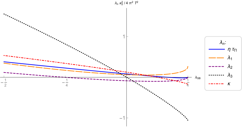
Figure 2: Second-order coefficients $\lambda_{n}=\{\eta\tau_{\Pi},\lambda_{1},\lambda_{2},\lambda_{3},\kappa\}$ of Gauss-Bonnet holographic liquid, in units of $4\pi^{2}T^{2}/\kappa_{5}^{2}$, as functions of $\lambda_{\scriptscriptstyle GB}$.

While $\lambda_{1}$ is positive-definite for all $\lambda_{\scriptscriptstyle GB}$, other coefficients can have either sign.

The derivatives of the coefficients with respect to $\lambda_{\scriptscriptstyle GB}$ are shown in Fig. 3. The coefficients $\lambda_{3}$ and $\kappa$ are monotonically decreasing functions of $\lambda_{\scriptscriptstyle GB}$ as can be seen from

$$\frac{\kappa^{2}_{5}}{4\pi^{2}T^{2}}\frac{\partial\lambda_{3}}{\partial\lambda_{\scriptscriptstyle GB}}=-\frac{1+15\gamma_{\scriptscriptstyle GB}+12\gamma_{\scriptscriptstyle GB}^{2}}{2\sqrt{2}\gamma_{\scriptscriptstyle GB}(1+\gamma_{\scriptscriptstyle GB})^{3/2}}<0,$$ (181)

$$\frac{\kappa^{2}_{5}}{4\pi^{2}T^{2}}\frac{\partial\kappa}{\partial\lambda_{\scriptscriptstyle GB}}=-\frac{1+8\gamma_{\scriptscriptstyle GB}+6\gamma_{\scriptscriptstyle GB}^{2}}{4\sqrt{2}\gamma_{\scriptscriptstyle GB}(1+\gamma_{\scriptscriptstyle GB})^{3/2}}<0,$$ (182)

whereas the coefficients $\eta\tau_{\Pi}$, $\lambda_{1}$ and $\lambda_{2}$ are not.

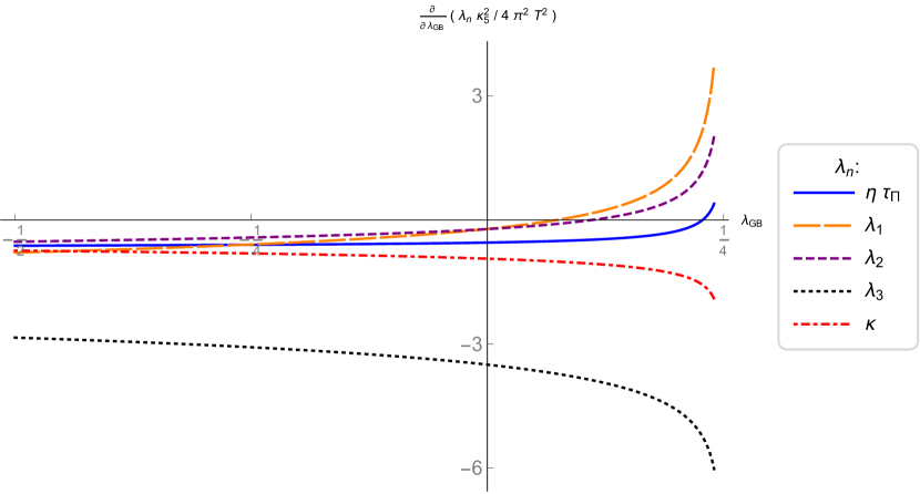
Figure 3: Derivatives of the second-order coefficients $\lambda_{n}=\{\eta\tau_{\Pi},\lambda_{1},\lambda_{2},\lambda_{3},\kappa\}$ with respect to $\lambda_{\scriptscriptstyle GB}$, in units of $4\pi^{2}T^{2}/\kappa_{5}^{2}$, as functions of $\lambda_{\scriptscriptstyle GB}$.

5 Charge diffusion from higher-derivative Einstein-Maxwell-Gauss-Bonnet action

Can first-order transport coefficients other than shear viscosity be tuned to zero with a suitable choice of higher derivative bulk terms, and can this be done simultaneously with tuning to zero the viscosity? In this section, we compute non-perturbative corrections to the well known result for the $U(1)$ charge diffusion constant at infinite coupling Policastro:2002se in a hypothetical boundary theory dual to Einstein-Maxwell-Gauss-Bonnet gravity with the charge neutral black brane background (29).

5.1 The four-derivative action

We are interested in the four-derivative Einstein-Maxwell-Gauss-Bonnet action whose equations of motion involve at most second derivatives. Such theories were previously considered in refs. Anninos:2008sj ; Kats:2006xp , and in the context of an effective target-space heterotic string theory action in Gross:1986mw . The higher-derivative Maxwell terms may appear as a result of compactification, e.g. of a higher-dimensional Gauss-Bonnet action. Here we construct the necessary action directly.

We begin by considering the Einstein-Maxwell-Gauss-Bonnet theory with the most general four-derivative Maxwell field Lagrangian,

$$S=\frac{1}{2\kappa^{2}_{5}}\int d^{5}x\sqrt{-g}\left[R-2\Lambda+\mathcal{L}_{GB}\right]+\int d^{5}x\sqrt{-g}\mathcal{L}_{A},$$ (183)

where $\Lambda=-6/L^{2}$, the Gauss-Bonnet Lagrangian $\mathcal{L}_{GB}$ is given by Eq. (16), and

$$\mathcal{L}_{A}=-\frac{1}{4}F_{\mu\nu}F^{\mu\nu}+\alpha_{4}RF_{\mu\nu}F^{\mu\nu}+\alpha_{5}R^{\mu\nu}F_{\mu\rho}F_{\nu}^{~{}\rho}+\alpha_{6}R^{\mu\nu\rho\sigma}F_{\mu\nu}F_{\rho\sigma}+\alpha_{7}\left(F_{\mu\nu}F^{\mu\nu}\right)^{2}$$

$$+\alpha_{8}\nabla_{\mu}F_{\rho\sigma}\nabla^{\mu}F^{\rho\sigma}+\alpha_{9}\nabla_{\mu}F_{\rho\sigma}\nabla^{\rho}F^{\mu\sigma}+\alpha_{10}\nabla_{\mu}F^{\mu\nu}\nabla^{\rho}F_{\rho\nu}+\alpha_{11}F^{\mu\nu}F_{\nu\rho}F^{\rho\sigma}F_{\sigma\mu}.$$ (184)

The coupled equations of motion for $g_{\mu\nu}$ and $A_{\mu}$ following from the action (183) are written in Appendix E. To make third- and fourth-order derivatives of the fields vanish in the equations of motion (266), we must impose the following constraints on the coefficients $\alpha_{n}$

$$\alpha_{4}=\alpha_{6}, 8\alpha_{4}+\alpha_{5}-4\alpha_{6}=0,$$ (185)

$$4\alpha_{4}+\alpha_{5}-2\alpha_{8}-\alpha_{9}=0, 2\alpha_{8}+\alpha_{9}+\alpha_{10}=0.$$ (186)

The second constraint in (186) also ensures that all higher-order derivatives vanish from the Maxwell’s equations (267). The constraints can be solved by setting

$$\alpha_{6}=\alpha_{4}, \alpha_{5}=-4\alpha_{4}, \alpha_{9}=-2\alpha_{8}, \alpha_{10}=0.$$ (187)

Coefficients $\alpha_{7}$ and $\alpha_{11}$ are left undetermined by this procedure. The vector field Lagrangian becomes

$$\mathcal{L}_{A}= -\frac{1}{4}F_{\mu\nu}F^{\mu\nu}+\beta_{1}L^{2}\left(RF_{\mu\nu}F^{\mu\nu}-4R^{\mu\nu}F_{\mu\rho}F_{\nu}^{~{}\rho}+R^{\mu\nu\rho\sigma}F_{\mu\nu}F_{\rho\sigma}\right)$$

$$+\beta_{4}L^{2}\nabla_{\mu}F_{\rho\sigma}\left(\nabla^{\mu}F^{\rho\sigma}-2\nabla^{\rho}F^{\mu\sigma}\right)+\beta_{2}L^{2}\left(F_{\mu\nu}F^{\mu\nu}\right)^{2}+\beta_{3}L^{2}F^{\mu\nu}F_{\nu\rho}F^{\rho\sigma}F_{\sigma\mu},$$ (188)

where we have defined the dimensionless couplings $\beta_{1}\equiv\alpha_{4}/L^{2}$, $\beta_{2}\equiv\alpha_{7}/L^{2}$, $\beta_{3}\equiv\alpha_{11}/L^{2}$ and $\beta_{4}\equiv\alpha_{8}/L^{2}$. To simplify the Lagrangian further, we notice that the term proportional to $\beta_{4}$ can be rewritten as

$$\nabla_{\mu}F_{\rho\sigma}\left(\nabla^{\mu}F^{\rho\sigma}-2\nabla^{\rho}F^{\mu\sigma}\right)=-2\nabla^{\mu}\nabla^{\rho}A^{\sigma}\left(R^{\lambda}_{~{}\mu\rho\sigma}+R^{\lambda}_{~{}\rho\sigma\mu}+R^{\lambda}_{~{}\sigma\mu\rho}\right)A_{\lambda}=0,$$ (189)

hence the entire expression vanishes due to the cyclic property of the Riemann tensor. Thus the Lagrangian $\mathcal{L}_{A}$ leading to second-order equations of motion is given by

$$\mathcal{L}_{A}= -\frac{1}{4}F_{\mu\nu}F^{\mu\nu}+\beta_{1}L^{2}\left(RF_{\mu\nu}F^{\mu\nu}-4R^{\mu\nu}F_{\mu\rho}F_{\nu}^{~{}\rho}+R^{\mu\nu\rho\sigma}F_{\mu\nu}F_{\rho\sigma}\right)$$

$$+\beta_{2}L^{2}\left(F_{\mu\nu}F^{\mu\nu}\right)^{2}+\beta_{3}L^{2}F^{\mu\nu}F_{\nu\rho}F^{\rho\sigma}F_{\sigma\mu}.$$ (190)

Therefore, there are altogether four parameters, $\lambda_{\scriptscriptstyle GB}$, $\beta_{1}$, $\beta_{2}$ and $\beta_{3}$, entering the second-order equations of motion of the theory. One may wonder if a black hole (brane) solution with non-perturbative values of these parameters exists. The black brane metric (29) is automatically a solution of the theory when $A_{\mu}=0$. It is also possible to find perturbative corrections in $\beta_{1}$, $\beta_{2}$ and $\beta_{3}$ to the five-dimensional AdS-Reissner-Nordström metric. However, we were not able to find a generalization of the solution (29) with non-trivial $A_{\mu}$ and fully non-perturbative non-vanishing $\beta_{1}$, $\beta_{2}$ and $\beta_{3}$.

5.2 The $U(1)$ charge diffusion constant

To compute the charge diffusion constant in a hypothetical neutral liquid dual to the bulk action constructed in the previous section we follow the procedure outlined in Kovtun:2005ev . We begin by perturbing the trivial $A_{\mu}=0$ background vector field as $A_{\mu}\to A_{\mu}+\epsilon a_{\mu}$ and writing the electromagnetic field strength corresponding to the linearized perturbation as $F=\epsilon\text{d}a$. Given the trivial background $A_{\mu}=0$, the metric fluctuations decouple from $a_{\mu}$ and can be set to zero.

In the equations of motion, the terms proportional to $\alpha_{7}$ and $\alpha_{11}$ (i.e. $\beta_{2}$ and $\beta_{3}$) only contribute to quadratic or higher orders in the expansion in $\epsilon$. Hence, they will not contribute to the charge diffusion constant. The linearized equations obeyed by $a_{\mu}$ read

$$\nabla_{\nu}F^{\mu\nu} =4\beta_{1}L^{2}\nabla_{\nu}\left(RF^{\mu\nu}+R^{\mu\nu\rho\sigma}F_{\rho\sigma}-R^{\mu\rho}F_{\rho}^{~{}\nu}+R^{\nu\rho}F_{\rho}^{~{}\mu}\right).$$ (191)

Vector field fluctuations can be decomposed into transverse and longitudinal modes, with charge diffusion coming from the low-energy hydrodynamic excitations in the longitudinal sector. By choosing the spatial momentum along the $z$-direction, the relevant gauge-invariant variable in the longitudinal sector is

$$Z_{4}=\mathfrak{q}a_{0}+\mathfrak{w}a_{4}.$$ (192)

We use the variable $u=r_{+}^{2}/r^{2}$, with the boundary at $u=0$ and horizon at $u=1$. Then we impose the incoming wave boundary condition required for the calculation of retarded correlators Son:2002sd by writing

$$Z_{4}=\left(1-u^{2}\right)^{-i\mathfrak{w}/2}\mathcal{Z}_{4}(u)\,,$$ (193)

where the function $\mathcal{Z}_{4}(u)$ regular at the horizon can be found perturbatively in $\mu\ll 1$, with $\mathfrak{q}$ and $\mathfrak{w}$ scaling as $\mathfrak{w}\to\mu^{2}\mathfrak{w}$ and $\mathfrak{q}\to\mu\mathfrak{q}$. We find it useful to introduce a new variable ${\it w}$, so that $u=\sqrt{{\it w}^{2}-\gamma_{\scriptscriptstyle GB}^{2}}/\sqrt{1-\gamma_{\scriptscriptstyle GB}^{2}}$. The boundary is now at ${\it w}=\gamma_{\scriptscriptstyle GB}$ and horizon at ${\it w}=1$. At order $\mathcal{O}(\mu^{0})$, the function $\mathcal{Z}_{4}$ can be written as $\mathcal{Z}_{4}=C_{1}+C_{2}\,z({\it w})$, where $z({\it w})$ is a solution of the equation

$$\frac{d^{2}z}{d{\it w}^{2}}-\frac{48\beta_{1}\left({\it w}^{3}-\gamma_{\scriptscriptstyle GB}^{2}\right)-\gamma_{\scriptscriptstyle GB}^{2}\left(1-\gamma_{\scriptscriptstyle GB}^{2}\right)}{{\it w}\left({\it w}^{2}-\gamma_{\scriptscriptstyle GB}^{2}\right)\left(1-\gamma_{\scriptscriptstyle GB}^{2}+48\beta_{1}(1-{\it w})\right)}\frac{dz}{d{\it w}}=0.$$ (194)

We solve for $z({\it w})$ and impose the boundary conditions $z(\gamma_{\scriptscriptstyle GB})=1$ and $z(1)=0$. The constant $C_{2}$ can then be expressed as a function of $C_{1}$, $\mathfrak{w}$, $\mathfrak{q}$ and other parameters of the theory by substituting $z({\it w})$ into the original differential equation, expanding to order $\mathcal{O}(\mu^{2})$ and imposing regularity at the horizon.

The hydrodynamic quasinormal mode can be found by solving the equation $Z_{4}(\mathfrak{w},\mathfrak{q})=0$ at the boundary for $\mathfrak{w}$. The dispersion relation has the form

$$\mathfrak{w}=-i\mathcal{D}\mathfrak{q}^{2}+\mathcal{O}(\mathfrak{q}^{4})\,,$$ (195)

where $\mathcal{D}$ is the charge diffusion constant of the dual theory. For the Gauss-Bonnet coupling in the interval $\lambda_{\scriptscriptstyle GB}\in[0,1/4]$ ($1\geq\gamma_{\scriptscriptstyle GB}\geq 0$) we find

$$\mathcal{D}= ~{}\frac{(1+\gamma_{\scriptscriptstyle GB})(1+2\beta)\left(\beta+\sqrt{\beta^{2}-\gamma_{\scriptscriptstyle GB}^{2}}\right)}{6(\beta-1)\left[\beta\left(\beta+\sqrt{\beta^{2}-\gamma_{\scriptscriptstyle GB}^{2}}\right)-\gamma_{\scriptscriptstyle GB}^{2}\right]}\Biggl{\{}\sqrt{\left(1-\gamma_{\scriptscriptstyle GB}^{2}\right)\left(\beta^{2}-\gamma_{\scriptscriptstyle GB}^{2}\right)}\,\ln\left[\frac{\gamma_{\scriptscriptstyle GB}}{1+\sqrt{1-\gamma_{\scriptscriptstyle GB}^{2}}}\right]$$

$$-\left(\beta-\gamma_{\scriptscriptstyle GB}^{2}\right)\ln\left[\frac{\gamma_{\scriptscriptstyle GB}}{\beta+\sqrt{\beta^{2}-\gamma_{\scriptscriptstyle GB}^{2}}}\right]\Biggr{\}}\,,$$ (196)

where $\beta\equiv 1+48\beta_{1}$ and $\gamma_{\scriptscriptstyle GB}\equiv\sqrt{1-4\lambda_{\scriptscriptstyle GB}}$.

We can now consider various limits. For the two-derivative Maxwell field in Gauss-Bonnet background, i.e. for $\beta_{1}=0$ ($\beta=1$), we find the expression

$$\mathcal{D}=\frac{1}{2}\left(1+\sqrt{1-4\lambda_{\scriptscriptstyle GB}}\right).$$ (197)

For $\mathcal{N}=4$ SYM theory, where $\lambda_{\scriptscriptstyle GB}=0$ and $\beta_{1}=0$, Eq. (197) reproduces the well-known result Policastro:2002se ,

$$\mathcal{D}=1.$$ (198)

In the zero viscosity limit $\lambda_{\scriptscriptstyle GB}=1/4$ ($\gamma_{\scriptscriptstyle GB}=0$), Eq. (197) gives

$$\mathcal{D}=1/2.$$ (199)

In the presence of higher-derivative vector-field terms in the Lagrangian (5.1), we find the diffusion constant in the two important limits of $\lambda_{\scriptscriptstyle GB}$ to be

$$\lambda_{\scriptscriptstyle GB}=0: \mathcal{D}=\left(\frac{1+32\beta_{1}}{4\sqrt{6}\sqrt{\beta_{1}\left(1+24\beta_{1}\right)}}\right)\ln\left[1+48\beta_{1}+\sqrt{\left(1+48\beta_{1}\right)^{2}-1}\right],$$ (200)

$$\lambda_{\scriptscriptstyle GB}=1/4: \mathcal{D}=\left(\frac{1+32\beta_{1}}{96\beta_{1}}\right)\ln\left(1+48\beta_{1}\right).$$ (201)

From Eq. (201) one can see that for $\lambda_{\scriptscriptstyle GB}=1/4$, the diffusion constant $\mathcal{D}$ remains a real function of the parameter $\beta_{1}$ as long as $\beta_{1}>-1/48$ and, moreover, this function is strictly positive for all $\beta_{1}$ in that interval. In this sense, we cannot have vanishing shear viscosity and diffusion constant simultaneously. The diffusion constant can vanish for other values of $\lambda_{\scriptscriptstyle GB}$: for example, $\mathcal{D}=0$ for $\beta_{1}=-1/32$. However, such a solution for $\mathcal{D}$ is not smoothly connected to the theory which has a vanishing shear viscosity. More precisely, for any $\beta_{1}=-1/32+\epsilon$, where $\epsilon\ll 1$, $\mathcal{D}$ is complex near $\gamma_{\scriptscriptstyle GB}=0$.

6 Conclusions

Together with refs. Grozdanov:2015asa ; Grozdanov:2014kva ; Grozdanov:2016vgg , the present paper is an attempt at a comprehensive investigation of the second-order transport properties, energy-momentum tensor correlation functions and quasinormal spectrum in the Gauss-Bonnet holographic fluid in $D=3+1$ dimensions non-perturbatively in Gauss-Bonnet coupling $\lambda_{\scriptscriptstyle GB}$. The existence of a strongly coupled CFT dual to classical non-Einsteinian gravity such as Gauss-Bonnet gravity at finite $\lambda_{\scriptscriptstyle GB}$ would be an interesting alternative to the standard scenario of gauge-gravity duality. However, the work of Camanho et al. Camanho:2014apa appears to cast a serious doubt on such a possibility, reducing the status of the curvature-squared terms to that of a perturbative correction. At the same time, we have not found any obvious pathology in hydrodynamic properties of the hypothetical dual field theory at finite $\lambda_{\scriptscriptstyle GB}$.

The curvature-squared terms are interesting even as corrections to the Einstein’s gravity description of a dual field theory, the second-order nature of the Gauss-Bonnet equations of motion making it easier to search for the new features such as the extra poles of the correlators not seen at $\lambda_{\scriptscriptstyle GB}=0$. The analysis of gravitational quasinormal spectrum in ref. Grozdanov:2016vgg and in the present paper shows that the analytic structure of dual thermal correlators is qualitatively different depending on the sign of $\lambda_{\scriptscriptstyle GB}$ (understood as inverse coupling), with the $\lambda_{\scriptscriptstyle GB}<0$ case showing "normal" (e.g. qualitatively similar to ${\cal N}=4$ SYM at finite ’t Hooft coupling and infinite $N_{c}$ and having a potential to connect to the kinetic regime) features, and the $\lambda_{\scriptscriptstyle GB}>0$ case demonstrating various anomalies (whose precise meaning remains to be understood, possibly invoking various monotonicity arguments). On the other hand, constraints on $\lambda_{\scriptscriptstyle GB}$ may come from different considerations such as the recent argument for $\lambda_{\scriptscriptstyle GB}>0$ in ref. Cheung:2016wjt based on unitarity. Fortunately, corrections coming from $R^{2}$ and $R^{4}$ higher derivative terms seem to be very similar Grozdanov:2016vgg in uncovering a qualitative picture of transport and other properties at large but finite coupling.

Appendix A Second-order transport coefficients of ${\cal N}=4$ SYM at weak and strong coupling

For the finite-temperature ${\cal N}=4$ $SU(N_{c})$ supersymmetric Yang-Mills (SYM) theory in $d=3+1$ dimensions in the limit of infinite $N_{c}$ and infinite ’t Hooft coupling $\lambda=g^{2}_{YM}N_{c}$, first- and second-order transport coefficients were computed, correspondingly, in Policastro:2001yc and Baier:2007ix ; Bhattacharyya:2008jc using methods of gauge-gravity and fluid-gravity dualities:

$$\eta =\frac{\pi}{8}N^{2}_{c}T^{3}\,,$$ (202)

$$\tau_{\Pi} =\frac{\left(2-\ln{2}\right)}{2\pi T}\,,\qquad\kappa=\frac{\eta}{\pi T}\,,\qquad\lambda_{1}=\frac{\eta}{2\pi T}\,,\qquad\lambda_{2}=-\frac{\eta\ln{2}}{\pi T}\,,\qquad\lambda_{3}=0\,.$$ (203)

Coupling constant corrections to the coefficients (202), (203) can be determined from the higher-derivative terms in the low-energy effective action of type IIB string theory

$$S=\frac{1}{2\kappa_{5}^{2}}\int d^{5}x\sqrt{-g}\left(R+\frac{12}{L^{2}}+\gamma\mathcal{W}\right),$$ (204)

where $\gamma=\alpha^{\prime 3}\zeta(3)/8$, $L$ is the AdS curvature scale, and the ratio $\alpha^{\prime}/L^{2}$ is related to the value of the ’t Hooft coupling $\lambda$ in ${\cal N}=4$ SYM via $\alpha^{\prime}/L^{2}=\lambda^{-1/2}$. The effective five-dimensional gravitational constant is connected to $N_{c}$ by $\kappa_{5}=2\pi/N_{c}$. The term $\mathcal{W}$ is given in terms of the Weyl tensor $C_{\mu\nu\rho\sigma}$ by

$$\mathcal{W}=C^{\alpha\beta\gamma\delta}C_{\mu\beta\gamma\nu}C_{\alpha}^{~{}\rho\sigma\mu}C^{\nu}_{~{}\rho\sigma\delta}+\frac{1}{2}C^{\alpha\delta\beta\gamma}C_{\mu\nu\beta\gamma}C_{\alpha}^{~{}\rho\sigma\mu}C^{\nu}_{~{}\rho\sigma\delta}.$$ (205)

Corrections to all first and second-order transport coefficients are known Buchel:2004di ; Benincasa:2005qc ; Buchel:2008sh ; Buchel:2008ac ; Buchel:2008bz ; Buchel:2008kd ; Saremi:2011nh ; Grozdanov:2014kva :

$$\eta =\frac{\pi}{8}N^{2}_{c}T^{3}\,\left(1+\frac{135\zeta(3)}{8}\,\lambda^{-3/2}+\ldots\,\right)\,,$$ (206)

$$\tau_{\Pi} =\frac{\left(2-\ln{2}\right)}{2\pi T}+\frac{375\zeta(3)}{32\pi T}\,\lambda^{-3/2}+\ldots\,,$$ (207)

$$\kappa =\frac{N_{c}^{2}T^{2}}{8}\left(1-\frac{5\zeta(3)}{4}\,\lambda^{-3/2}+\ldots\,\right)\,,$$ (208)

$$\lambda_{1} =\frac{N_{c}^{2}T^{2}}{16}\left(1+\frac{175\zeta(3)}{4}\,\lambda^{-3/2}+\ldots\,\right)\,,$$ (209)

$$\lambda_{2} =-\frac{N_{c}^{2}T^{2}}{16}\left(2\ln{2}+\frac{5\left(97+54\ln{2}\right)\zeta(3)}{8}\lambda^{-3/2}+\ldots\,\right),$$ (210)

$$\lambda_{3} =\frac{N_{c}^{2}T^{2}}{16}\,25\zeta(3)\,\lambda^{-3/2}+\ldots\,.$$ (211)

Leading order results for the third order coefficients $\theta_{1}$ and $\theta_{2}$ entering the hydrodynamic dispersion relations are known as well Grozdanov:2015kqa :

$$\theta_{1} =\frac{N_{c}^{2}T}{32\pi}+O(\gamma)\,,$$ (212)

$$\theta_{2} =\frac{N_{c}^{2}T}{384\pi}\left(22-\frac{\pi^{2}}{12}-18\ln{2}+\ln^{2}2\right)+O(\gamma)\,.$$ (213)

Additional explicit results for the linear combinations of ${\cal N}=4$ SYM third order coefficients can be found in ref. Grozdanov:2015kqa . Other coupling constant corrections to the results at infinitely strong t’Hooft coupling in finite temperature ${\cal N}=4$ SYM include corrections to the entropy Gubser:1998nz ; Pawelczyk:1998pb , photon emission rate Hassanain:2012uj , and poles of the retarded correlator of the energy-momentum tensor Stricker:2013lma .

In ${\cal N}=4$ SYM at weak coupling, the shear viscosity has been computed in ref. Huot:2006ys . The second-order transport coefficients in various theories at weak coupling (QCD with either 0 or 3 flavours, QED, $\lambda\phi^{4}$) were determined by York and Moore York:2008rr . In conformal kinetic theory (at weak coupling) one finds $2\eta\tau_{\Pi}+\lambda_{2}=0$ Baier:2007ix ; York:2008rr ; Betz:2008me . Curiously, in the theories considered in York:2008rr the Haack-Yarom relation (7) at weak coupling can be expressed as

$$H=\frac{4\eta^{2}}{\epsilon+P}\left(C_{1}-C_{2}\right),$$ (214)

where $\epsilon$ and $P$ are energy density and pressure, correspondingly, and $C_{1}$ and $C_{2}$ are theory-specific constants (e.g. $C_{1}\approx 6.10517$, $C_{2}\approx 6.13264$ for $\lambda\phi^{4}$ theory). It appears that at weak coupling one finds $H\neq 0$ also in other (nearly conformal) examples GMoore . It would be interesting to compute $H(\lambda)$ directly in ${\cal N}=4$ SYM at weak coupling. Another interesting finding of ref. York:2008rr is that at weak coupling the coefficients $\kappa$ and $\lambda_{3}$ vanish to order $\propto T^{2}/\lambda^{4}$ (but may be non-zero at $\propto T^{2}/\lambda^{2}$). We note that $\lambda_{3}=0$ in the limit $\lambda\rightarrow\infty$ but has a non-trivial coupling dependence as can be seen from (211).

Appendix B Notations and conventions in formulas of relativistic hydrodynamics

For the convenience of the reader, here we compare notations and sign conventions used in the present paper with those used in refs. Baier:2007ix , York:2008rr , Grozdanov:2014kva , Bhattacharyya:2008jc , Bhattacharya:2012zx , Haack:2008xx , Shaverin:2012kv .

Notations and conventions used in the present paper and in refs. Baier:2007ix , York:2008rr , Grozdanov:2014kva .

The energy-momentum tensor of a neutral conformal relativistic fluid considered in the Landau frame is written as

$$T^{ab}=\varepsilon u^{a}u^{b}+P\Delta^{ab}+\Pi^{ab},$$ (215)

where $\Delta^{ab}\equiv g^{ab}+u^{a}u^{b}$, pressure $P$ and energy density $\varepsilon$ are related by the conformal fluid equation of state in four dimensions, $P=\varepsilon/3$, and

$$\Pi^{ab}= ~{}-\eta\sigma^{ab}+\eta\tau_{\Pi}\left[{}^{\langle}D\sigma^{ab\rangle}+\frac{1}{d-1}\sigma^{ab}\left(\nabla\cdot u\right)\right]+\kappa\left[R^{\langle ab\rangle}-(d-2)u_{c}R^{c\langle ab\rangle d}u_{d}\right]$$

$$+\lambda_{1}\sigma^{\langle a}_{~{}~{}c}\sigma^{b\rangle c}+\lambda_{2}\sigma^{\langle a}_{~{}~{}c}\Omega^{b\rangle c}+\lambda_{3}\Omega^{\langle a}_{~{}~{}c}\Omega^{b\rangle c},$$ (216)

where $D\equiv u^{a}\nabla_{a}$. We use the following definitions (in our case, $d=4$)

$$A^{\langle ab\rangle}\equiv\frac{1}{2}\Delta^{ac}\Delta^{bd}\left(A_{cd}+A_{dc}\right)-\frac{1}{d-1}\Delta^{ab}\Delta^{cd}A_{cd}\equiv{}^{\langle}A^{ab\rangle},$$ (217)

where by construction the resulting tensors are transverse, $u_{a}A^{\langle ab\rangle}=0$, traceless, $g_{ab}A^{\langle ab\rangle}=0$, and symmetric. The tensor $\sigma^{ab}$ is a symmetric, transverse and traceless tensor involving first derivatives of the velocity field

$$\sigma^{ab}=2{}^{\langle}\nabla^{a}u^{b\rangle}.$$ (218)

The vorticity $\Omega^{\mu\nu}$ is defined as an anti-symmetric, transverse and traceless one-derivative tensor

$$\Omega^{ab}=\frac{1}{2}\Delta^{ac}\Delta^{bd}\left(\nabla_{c}u_{d}-\nabla_{d}u_{c}\right).$$ (219)

The Haack-Yarom relation in our notations reads

$$2\eta\tau_{\Pi}-4\lambda_{1}-\lambda_{2}=0\,,$$ (220)

whereas the conformal kinetic theory result York:2008rr is

$$2\eta\tau_{\Pi}+\lambda_{2}=0\,.$$ (221)

Notations and conventions used in refs. Bhattacharyya:2008jc , Bhattacharya:2012zx

We label the objects used in refs. Bhattacharyya:2008jc ; Bhattacharya:2012zx with the letter "R", e.g.

$$\sigma^{\mu\nu}_{R}=P^{\mu\alpha}P^{\nu\beta}\partial_{(\alpha}u_{\beta)}-\frac{1}{3}\partial_{\alpha}u^{\alpha}\,,$$ (222)

where $P^{\mu\nu}=\eta^{\mu\nu}+u^{\mu}u^{\nu}$, $a^{(\alpha}b^{\beta)}=(a^{\alpha}b^{\beta}+a^{\beta}b^{\alpha})/2$, $a^{[\alpha}b^{\beta]}=(a^{\alpha}b^{\beta}-a^{\beta}b^{\alpha})/2$. The vorticity is defined as

$$\omega^{\mu\nu}_{R}=-\frac{1}{2}P^{\mu\alpha}P^{\nu\beta}\left(\partial_{\alpha}u_{\beta}-\partial_{\beta}u_{\alpha}\right).$$ (223)

It is clear that $\sigma_{\mu\nu}^{R}=\frac{1}{2}\sigma_{\mu\nu}$ and $\omega_{\mu\nu}^{R}=-\Omega_{\mu\nu}$. The energy-momentum tensor is written as

$$T^{\mu\nu}=\varepsilon u^{\mu}u^{\nu}+pP^{\mu\nu}+\Pi^{\mu\nu},$$ (224)

where

$$\Pi^{\mu\nu}= ~{}-\eta\sigma^{\mu\nu}_{R}+\dots+\lambda_{2}^{R}\sigma^{\langle\mu}_{~{}~{}\lambda,R}\omega^{\nu\rangle\lambda}_{R}+\cdots\,.$$ (225)

Therefore, $\lambda_{2}^{R}=-2\lambda_{2}$. Similar relations hold for other coefficients. In summary,

$$\eta =\eta^{R}\,,$$ (226)

$$\eta\tau_{\Pi} =\frac{1}{2}\tau_{R}\,,$$ (227)

$$\kappa =\kappa_{1}^{R}=\frac{1}{2}\kappa_{R}\,,$$ (228)

$$\lambda_{1} =\frac{1}{4}\lambda_{1}^{R}\,,$$ (229)

$$\lambda_{2} =-\frac{1}{2}\lambda_{2}^{R}\,,$$ (230)

$$\lambda_{3} =-\lambda_{3}^{R}\,.$$ (231)

The Haack-Yarom relation reads

$$2\tau^{R}-2\lambda_{1}^{R}+\lambda_{2}^{R}=0\,$$ (232)

or, equivalently, for liquids with $\lambda_{1}^{R}=\kappa^{R}$ (i.e. $\kappa=2\lambda_{1}$ in our notations)

$$2\tau^{R}-2\kappa^{R}+\lambda_{2}^{R}=0\,.$$ (233)

The conformal kinetic theory result York:2008rr in these notations reads

$$2\tau^{R}-\lambda_{2}^{R}=0\,.$$ (234)

Notations and conventions used in refs. Haack:2008xx , Shaverin:2012kv

In ref. Haack:2008xx , the tensor $\sigma^{\mu\nu}_{HY}$ is defined as

$$\sigma^{\mu\nu}_{HY}=2{}^{\langle}\nabla^{\mu}u^{\nu\rangle}$$ (235)

and the vorticity $\omega^{\mu\nu}_{HY}$ is

$$\omega^{\mu\nu}_{HY}=\frac{1}{2}P^{\mu\lambda}P^{\nu\sigma}\left(\nabla_{\lambda}u_{\sigma}-\nabla_{\sigma}u_{\lambda}\right),$$ (236)

which coincides with the definitions in Baier:2007ix , York:2008rr , Grozdanov:2014kva . The term in the expression for the energy-momentum tensor multiplying $\lambda_{2}^{HY}$,

$$T^{\mu\nu}= ~{}\lambda_{2}^{HY}\,\sigma^{\langle\mu}_{~{}~{}\lambda,\mbox{\tiny{HY}}}\omega^{\lambda\nu\rangle}_{HY}+\cdots\,,$$ (237)

is different in the order of indices from the one used in Baier:2007ix , York:2008rr , Grozdanov:2014kva , where $T^{ab}=\lambda_{2}\,\sigma^{\langle a}_{~{}~{}c}\Omega^{b\rangle c}+\dots$, and, since vorticity is antisymmetric, we could have concluded that $\lambda_{2}=-\lambda_{2}^{HY}$ (?). Then the original Haack-Yarom relation as stated in ref. Haack:2008xx ,

$$2\eta^{HY}\tau_{\Pi}^{HY}-4\lambda_{1}^{HY}-\lambda_{2}^{HY}=0\,,$$ (238)

would translate to our notations as (all other coefficients coincide with ours)

$$2\eta\tau_{\Pi}-4\lambda_{1}+\lambda_{2}=0\,\;\;\mbox{\bf(incorrect)}$$ (239)

which does not agree with Eq. (220) and is difficult to reconcile e.g. with the explicit results for ${\cal N}=4$ SYM given by (202) - (203). We believe that there is a typo in ref. Haack:2008xx , either in the arrangement of indices (it should be the same as in Baier:2007ix , York:2008rr , Grozdanov:2014kva ) or, alternatively, in the definition of vorticity (it should have an extra minus sign in front), or perhaps in the sign in front of $\lambda_{2}$ in the equation (238). The same observation has been recently made in ref. Haehl:2015pja . Correcting this typo, we have $\lambda_{2}=\lambda_{2}^{HY}$ and then notations in Haack:2008xx would give the same signs of transport coefficients as the ones in refs. Baier:2007ix , York:2008rr , Grozdanov:2014kva .

We note that in the paper by Shaverin and Yarom Shaverin:2012kv , the notations for $\sigma^{\mu\nu}_{SY}$, vorticity $\omega^{\mu\nu}_{SY}$ and their coupling $\lambda_{2}^{SY}\,\sigma^{\langle\mu}_{~{}~{}\alpha,\mbox{\tiny{SY}}}\omega^{\alpha\nu\rangle}_{SY}$ are the same as in ref. Haack:2008xx . The relations between our transport coefficients (i.e. the ones in Baier:2007ix , York:2008rr , Grozdanov:2014kva ) and the ones used in Shaverin:2012kv are

$$\eta^{SY}=\eta\,,$$ (240)

$$\lambda_{0}^{SY}=\eta\tau_{\Pi}\,,$$ (241)

$$\lambda_{1}^{SY}=\lambda_{1}\,,$$ (242)

$$\lambda_{2}^{SY}=-\lambda_{2}\,,$$ (243)

$$\lambda_{3}^{SY}=\lambda_{3}\,.$$ (244)

The Haack-Yarom relation as written in Shaverin:2012kv reads

$$-2\lambda_{0}^{SY}+4\lambda_{1}^{SY}-\lambda_{2}^{SY}=0\,,$$ (245)

which translates in our notations into Eq. (220), as expected.

Appendix C Boundary conditions at the horizon in the hydrodynamic regime

In this Appendix, we clarify the procedure of imposing the incoming wave boundary condition at the horizon on a (gauge-invariant) fluctuation $Z$ given by a perturbative series in the hydrodynamic regime ($\mathfrak{w}\ll 1$ and $\mathfrak{q}\ll 1$). Consider such a solution $Z_{1}$ near the horizon $u=1$:

$$Z_{1}=(1-u)^{-i\mathfrak{w}/2}F(u,\mathfrak{w})\,,$$ (246)

where $\mathfrak{q}$ is ignored for simplicity. Here, the function $F$ (regular at $u=1$ by Fröbenius construction) is found perturbatively as a series in $\mathfrak{w}\ll 1$,

$$F(u,\mathfrak{w})=F_{0}(u)+\mathfrak{w}F_{1}(u)+\mathfrak{w}^{2}F_{2}(u)+\cdots\,,$$ (247)

where $F_{i}(u)$ satisfy the equation of motion obeyed by $Z$ to a given order in $\mathfrak{w}$, with $F_{i}(1)=S_{i}$ for $i\geq 0$, and $S_{i}$ are constants independent of $u$ and $\mathfrak{w}$. Now consider another solution, $Z_{2}$, near $u=1$,

$$Z_{2}=(1-u)^{-i\mathfrak{w}/2}C(\mathfrak{w})G(u,\mathfrak{w})\,,$$ (248)

where $C(\mathfrak{w})$ is a function of $\mathfrak{w}$ only, and $G$ is found perturbatively by solving the differential equation obeyed by $Z$ by a series in $\mathfrak{w}\ll 1$,

$$G(u,\mathfrak{w})=G_{0}(u)+\mathfrak{w}G_{1}(u)+\mathfrak{w}^{2}G_{2}(u)+\cdots\,,$$ (249)

$$G_{0}(1)=1,G_{i}(1)=0\;\mbox{for}\;i>0\,.$$ (250)

Now, the solution $Z_{1}$ with its boundary condition at the horizon can always be written as $Z_{2}$ with the appropriate choice of the function $C(\mathfrak{w})$. Indeed, expanding $C(\mathfrak{w})$ in Taylor series at $\mathfrak{w}=0$, $C(\mathfrak{w})=C(0)+C^{\prime}(0)\mathfrak{w}+...$, we get

$$Z_{2} =(1-u)^{-i\mathfrak{w}/2}\Biggl{\{}G_{0}(u)C(0)+\mathfrak{w}\left[G_{0}(u)C^{\prime}(0)+G_{1}(u)C(0)\right]$$ (251)

$$+\mathfrak{w}^{2}\left[\frac{1}{2}\,G_{0}(u)C^{\prime\prime}(0)\,+G_{1}(u)C^{\prime}(0)+C(0)G_{2}(u)\right]+O(\mathfrak{w}^{3})\Biggr{\}}\,.$$

Comparing $Z_{2}$ and $Z_{1}$ at $u=1$, we identify $C(0)=S_{0}$, $C^{\prime}(0)=S_{1}$, and so on. In other words, nontrivial boundary conditions at the horizon for functions $F_{i}$ of the solution $Z_{1}$ can be understood as coefficients of the small-$\mathfrak{w}$ expansion of a multiplicative factor $C(\mathfrak{w})$. Since in holography we work with bulk solutions normalized to one at the boundary, i.e. $f_{k}(u)=Z(u)/Z(\epsilon)$, such a multiplicative factor cancels. This justifies always using the expansion (249) with the boundary conditions (250).

Appendix D The coefficients $A_{i}$ and $B_{i}$ of the differential equation (47)

Scalar channel

$$A_{1}=\, -\frac{1}{u}-u\left[\frac{1}{\left(\gamma_{\scriptscriptstyle GB}^{2}-1\right)\left(1-u^{2}\right)^{2}+1-u^{2}}+\frac{1}{\left(1-u^{2}\right)\sqrt{\gamma_{\scriptscriptstyle GB}^{2}-\left(\gamma_{\scriptscriptstyle GB}^{2}-1\right)u^{2}}}\right],$$ (252)

$$B_{1}=\, \frac{(\gamma_{\scriptscriptstyle GB}-1)(\gamma_{\scriptscriptstyle GB}+1)^{2}\left(3\left(\gamma_{\scriptscriptstyle GB}^{2}-1\right)u^{2}-\gamma_{\scriptscriptstyle GB}^{2}\right)\left(-\gamma_{\scriptscriptstyle GB}^{2}+\left(\gamma_{\scriptscriptstyle GB}^{2}-1\right)u^{2}+U\right)}{4u\left(\gamma_{\scriptscriptstyle GB}^{2}-\left(\gamma_{\scriptscriptstyle GB}^{2}-1\right)u^{2}\right)^{3/2}\left(-\gamma_{\scriptscriptstyle GB}^{2}+\left(\gamma_{\scriptscriptstyle GB}^{2}-1\right)u^{2}+2U-1\right)}\mathfrak{q}^{2}$$

$$+\frac{\left(\gamma_{\scriptscriptstyle GB}^{2}-1\right)^{2}\left(-\gamma_{\scriptscriptstyle GB}^{2}+\left(\gamma_{\scriptscriptstyle GB}^{2}-1\right)u^{2}+U\right)}{4u(U-1)\sqrt{\gamma_{\scriptscriptstyle GB}^{2}-\left(\gamma_{\scriptscriptstyle GB}^{2}-1\right)u^{2}}\left(-\gamma_{\scriptscriptstyle GB}^{2}+\left(\gamma_{\scriptscriptstyle GB}^{2}-1\right)u^{2}+2U-1\right)}\mathfrak{w}^{2},$$ (253)

Shear channel

$$A_{2}=\, -\frac{2\gamma_{\scriptscriptstyle GB}^{4}(\gamma_{\scriptscriptstyle GB}+1)\left[\frac{1}{2}\left(1-\gamma_{\scriptscriptstyle GB}^{2}\right)\left(u^{2}-1\right)(U-2)+U-1\right]}{u(U-1)U^{3}\left[\gamma_{\scriptscriptstyle GB}^{2}(\gamma_{\scriptscriptstyle GB}+1)(U-1)\mathfrak{q}^{2}-\left(\gamma_{\scriptscriptstyle GB}^{2}-1\right)U^{2}\mathfrak{w}^{2}\right]}\mathfrak{q}^{2}$$ (254)

$$-\frac{\left(1-\gamma_{\scriptscriptstyle GB}^{2}\right)\left(\gamma_{\scriptscriptstyle GB}^{4}+\left(1-\gamma_{\scriptscriptstyle GB}^{2}\right)^{2}u^{4}-2\left(1-\gamma_{\scriptscriptstyle GB}^{2}\right)u^{2}\left(U-\gamma_{\scriptscriptstyle GB}^{2}\right)-\gamma_{\scriptscriptstyle GB}^{2}U\right)}{u(U-1)U\left[\gamma_{\scriptscriptstyle GB}^{2}(\gamma_{\scriptscriptstyle GB}+1)(U-1)\mathfrak{q}^{2}-\left(\gamma_{\scriptscriptstyle GB}^{2}-1\right)U^{2}\mathfrak{w}^{2}\right]}\mathfrak{w}^{2},$$ (255)

$$B_{2}=\, \frac{\gamma_{\scriptscriptstyle GB}^{2}(\gamma_{\scriptscriptstyle GB}+1)(U+1)}{4u\left(u^{2}-1\right)U^{2}}\mathfrak{q}^{2}+\frac{\left(U^{2}+2U+1\right)}{4u\left(u^{2}-1\right)^{2}}\mathfrak{w}^{2},$$ (256)

Sound channel

$$A_{3}=\, \frac{3}{2u}+\frac{3(\gamma_{\scriptscriptstyle GB}-1)\left[\left(\gamma_{\scriptscriptstyle GB}^{2}-1\right)u^{2}-\gamma_{\scriptscriptstyle GB}^{2}\right]\left[\left(\gamma_{\scriptscriptstyle GB}^{2}-1\right)u^{2}(5U-7)-5\gamma_{\scriptscriptstyle GB}^{2}(U-1)\right]}{2u(U-1)U^{2}D_{1}}\mathfrak{w}^{2}$$

$$+\frac{\left(\gamma_{\scriptscriptstyle GB}^{2}-1\right)^{2}u^{4}\left(-3\gamma_{\scriptscriptstyle GB}^{2}+5U-7\right)+\gamma_{\scriptscriptstyle GB}^{2}\left(\gamma_{\scriptscriptstyle GB}^{2}-1\right)u^{2}\left(18\gamma_{\scriptscriptstyle GB}^{2}-13U+10\right)}{2u(U-1)U^{2}D_{1}}\mathfrak{q}^{2}$$

$$-\frac{15\gamma_{\scriptscriptstyle GB}^{4}\left(\gamma_{\scriptscriptstyle GB}^{2}-2U+1\right)}{2u(U-1)U^{2}D_{1}}\mathfrak{q}^{2},$$ (257)

$$B_{3}= ~{}\frac{\left(\gamma_{\scriptscriptstyle GB}^{2}-1\right)^{2}}{D_{0}}\biggr{\{}\,12(\gamma_{\scriptscriptstyle GB}-1)^{2}\gamma_{\scriptscriptstyle GB}^{2}(\gamma_{\scriptscriptstyle GB}+1)\mathfrak{q}^{2}u^{5}-4(\gamma_{\scriptscriptstyle GB}-1)\gamma_{\scriptscriptstyle GB}^{2}\mathfrak{q}^{2}u^{3}\left(3\gamma_{\scriptscriptstyle GB}^{2}-7U+4\right)$$

$$+\left(\gamma_{\scriptscriptstyle GB}^{2}-1\right)^{3}\mathfrak{q}^{2}u^{6}\left(3(\gamma_{\scriptscriptstyle GB}-1)\mathfrak{w}^{2}+\mathfrak{q}^{2}\right)$$

$$-u^{2}\gamma_{\scriptscriptstyle GB}^{2}\left(\gamma_{\scriptscriptstyle GB}^{2}-1\right)\left[\mathfrak{q}^{4}\left(\gamma_{\scriptscriptstyle GB}^{2}+2U\right)+(\gamma_{\scriptscriptstyle GB}-1)\mathfrak{q}^{2}\mathfrak{w}^{2}\left(9\gamma_{\scriptscriptstyle GB}^{2}-4U\right)-6(\gamma_{\scriptscriptstyle GB}-1)^{2}U\mathfrak{w}^{4}\right]$$

$$+\left(\gamma_{\scriptscriptstyle GB}^{2}-1\right)^{2}u^{4}\left[\mathfrak{q}^{4}\left(3\gamma_{\scriptscriptstyle GB}^{2}(U-2)+U\right)+2(\gamma_{\scriptscriptstyle GB}-1)\mathfrak{q}^{2}U\mathfrak{w}^{2}-3(\gamma_{\scriptscriptstyle GB}-1)^{2}U\mathfrak{w}^{4}\right]$$

$$-3\gamma_{\scriptscriptstyle GB}^{4}\left[\mathfrak{q}^{4}\left(\gamma_{\scriptscriptstyle GB}^{2}(U-2)+U\right)+2(\gamma_{\scriptscriptstyle GB}-1)\mathfrak{q}^{2}\mathfrak{w}^{2}\left(U-\gamma_{\scriptscriptstyle GB}^{2}\right)+(\gamma_{\scriptscriptstyle GB}-1)^{2}U\mathfrak{w}^{4}\right]\,\,\biggr{\}},$$ (258)

where we have defined

$$D_{1} \equiv\left(\gamma_{\scriptscriptstyle GB}^{2}-1\right)u^{2}\left(3(\gamma_{\scriptscriptstyle GB}-1)\mathfrak{w}^{2}+\mathfrak{q}^{2}\right)+3\gamma_{\scriptscriptstyle GB}^{2}\left(\mathfrak{q}^{2}(U-1)-(\gamma_{\scriptscriptstyle GB}-1)\mathfrak{w}^{2}\right),$$

$$D_{0} \equiv 4(\gamma_{\scriptscriptstyle GB}-1)u(U-1)^{2}U^{3}D_{1}.$$ (259)

In the above expressions, we used $U^{2}=u^{2}+\gamma_{\scriptscriptstyle GB}^{2}-u^{2}\gamma_{\scriptscriptstyle GB}^{2}$, as well as the dimensionless frequency and momentum (46), where the Hawking temperature is given by Eq. (33). Sometimes it is preferable to use the original radial coordinate $r$. For convenience, we write here the equation for the scalar fluctuation $Z_{1}$ in this variable:

$$P_{2}Z_{1}^{\prime\prime}+P_{1}Z_{1}^{\prime}+P_{0}Z_{1}=0,$$ (260)

where the coefficients are given by

$$P_{2}=rf\left(\lambda_{\scriptscriptstyle GB}f^{\prime}-r\right),$$ (261)

$$P_{1}=rf^{\prime}\left(\lambda_{\scriptscriptstyle GB}f^{\prime}-r\right)-3rf+\lambda_{\scriptscriptstyle GB}f\left(rf^{\prime\prime}+2f^{\prime}\right),$$ (262)

$$P_{0}=\frac{2}{f\left(1+\sqrt{1-4\lambda_{\scriptscriptstyle GB}}\right)}\biggr{[}r\omega^{2}\left(\lambda_{\scriptscriptstyle GB}f^{\prime}-r\right)-\left(1+\sqrt{1-4\lambda_{\scriptscriptstyle GB}}\right)f^{2}\left(\lambda_{\scriptscriptstyle GB}f^{\prime\prime}-1\right)$$

$$~{}~{}~{}~{}~{}+\frac{1}{2}\left(1+\sqrt{1-4\lambda_{\scriptscriptstyle GB}}\right)f\left(f^{\prime\prime}\left(r^{2}-\lambda_{\scriptscriptstyle GB}q^{2}\right)-2\lambda_{\scriptscriptstyle GB}f^{\prime 2}+4rf^{\prime}+q^{2}-12r^{2}\right)\biggr{]}\,,$$ (263)

where $f(r)$ is given by Eq. (30). To solve Eq. (260) with the incoming wave boundary condition at the horizon, it is convenient to write the solution as

$$Z_{1}=\tilde{f}(r)^{-i\mathfrak{w}/2}\left(1+g(r)\right),$$ (264)

where

$$\tilde{f}(r)=\frac{1}{2\lambda_{\scriptscriptstyle GB}}\left[1-\sqrt{1-4\lambda_{\scriptscriptstyle GB}\left(1-\left(r_{+}/r\right)^{4}\right)}\right].$$ (265)

This coordinate is more convenient for taking the limit of zero temperature.

Appendix E Equations of motion of Einstein-Maxwell-Gauss-Bonnet gravity

The equations of motion of Einstein-Maxwell-Gauss-Bonnet gravity following from the action (183) form a system of two coupled PDEs:

$$R_{\mu\nu}-\frac{1}{2}g_{\mu\nu}R+g_{\mu\nu}\Lambda=\mathcal{T}^{GB}_{\mu\nu}+2\kappa^{2}_{5}\mathcal{T}^{A}_{\mu\nu},$$ (266)

$$\nabla_{\nu}F^{\mu\nu}=4\alpha_{4}\nabla_{\nu}\left(RF^{\mu\nu}\right)+2\alpha_{5}\nabla_{\nu}\left(R^{\mu\rho}F_{\rho}^{~{}\nu}-R^{\nu\rho}F_{\rho}^{~{}\mu}\right)+4\alpha_{6}\nabla_{\nu}\left(R^{\alpha\beta\mu\nu}F_{\alpha\beta}\right)$$

$$+8\alpha_{7}\nabla_{\nu}\left(F_{\alpha\beta}F^{\alpha\beta}F^{\mu\nu}\right)-4\alpha_{8}\nabla_{\nu}\Box F^{\mu\nu}-2\alpha_{9}\nabla_{\nu}\nabla_{\rho}\left(\nabla^{\mu}F^{\rho\nu}-\nabla^{\nu}F^{\rho\mu}\right)$$

$$+2\alpha_{10}\nabla_{\nu}\left(\nabla^{\nu}\nabla_{\rho}F^{\rho\mu}-\nabla^{\mu}\nabla_{\rho}F^{\rho\nu}\right)+8\alpha_{11}\nabla_{\nu}\left(F^{\nu\rho}F_{\rho\sigma}F^{\sigma\mu}\right).$$ (267)

Here, the gravitational energy-momentum tensor term is given by

$$\mathcal{T}^{GB}_{\mu\nu}= \;\frac{\lambda_{\scriptscriptstyle GB}L^{2}}{4}g_{\mu\nu}\left(R^{2}-4R_{\mu\nu}R^{\mu\nu}+R_{\mu\nu\rho\sigma}R^{\mu\nu\rho\sigma}\right)$$

$$-\lambda_{\scriptscriptstyle GB}L^{2}\left(RR_{\mu\nu}-2R_{\mu\alpha}R_{\nu}^{~{}\alpha}-2R_{\mu\alpha\nu\beta}R^{\alpha\beta}+R_{\mu\alpha\beta\gamma}R_{\nu}^{\alpha\beta\gamma}\right),$$ (268)

and the Maxwell field contribution has the form

$$\mathcal{T}^{A}_{\mu\nu} =-\frac{1}{8}\left(g_{\mu\nu}F^{2}-4F_{\mu\lambda}F_{\nu}^{~{}\lambda}\right)$$

$$+\frac{\alpha_{4}}{2}\left[g_{\mu\nu}RF^{2}-4RF_{\mu\alpha}F_{\nu}^{~{}\alpha}-2R_{\mu\nu}F^{2}+2\nabla_{\mu}\nabla_{\nu}F^{2}-2g_{\mu\nu}\Box F^{2}\right]$$

$$+\frac{\alpha_{5}}{2}\left[g_{\mu\nu}R^{\alpha\beta}F_{\alpha\lambda}F_{\beta}^{~{}\lambda}-4R_{\mu\alpha}F_{\nu\beta}F^{\alpha\beta}-2R_{\alpha\beta}F_{\mu}^{~{}\alpha}F_{\nu}^{~{}\beta}-\Box\left(F_{\mu\alpha}F_{\nu}^{~{}\alpha}\right)-g_{\mu\nu}\nabla_{\alpha}\nabla_{\beta}\left(F^{\alpha}_{~{}\lambda}F^{\beta\lambda}\right)\right.$$

$$~{}~{}~{}~{}~{}~{}~{}\left.~{}+\nabla_{\alpha}\nabla_{\mu}\left(F_{\nu\beta}F^{\alpha\beta}\right)+\nabla_{\alpha}\nabla_{\nu}\left(F_{\mu\beta}F^{\alpha\beta}\right)\right]$$

$$+\frac{\alpha_{6}}{2}\left[g_{\mu\nu}R^{\alpha\beta\gamma\delta}F_{\alpha\beta}F_{\gamma\delta}-6R_{\mu\alpha\beta\gamma}F_{\nu}^{~{}\alpha}F^{\beta\gamma}-4\nabla^{\beta}\nabla^{\alpha}\left(F_{\mu\alpha}F_{\nu\beta}\right)\right]$$

$$+\frac{\alpha_{7}}{2}\left[g_{\mu\nu}\left(F^{2}\right)^{2}-8F^{2}F_{\mu\lambda}F_{\nu}^{~{}\lambda}\right]$$

$$+\frac{\alpha_{8}}{2}\left[g_{\mu\nu}\nabla_{\alpha}F_{\beta\gamma}\nabla^{\alpha}F^{\beta\gamma}-2\nabla_{\mu}F_{\alpha\beta}\nabla_{\nu}F^{\alpha\beta}-4\nabla_{\alpha}F_{\mu\beta}\nabla^{\alpha}F_{\nu}^{~{}\beta}+4\nabla_{\alpha}\left(\nabla_{\mu}F^{\alpha\beta}F_{\nu\beta}\right)\right.$$

$$~{}~{}~{}~{}~{}~{}~{}\left.~{}+4\nabla_{\alpha}\left(\nabla^{\alpha}F_{\mu}^{~{}\beta}F_{\nu\beta}\right)-4\nabla_{\alpha}\left(\nabla_{\mu}F_{\nu}^{~{}\beta}F^{\alpha}_{~{}\beta}\right)\right]$$

$$+\frac{\alpha_{9}}{2}\left[g_{\mu\nu}\nabla_{\alpha}F_{\beta\gamma}\nabla^{\beta}F^{\alpha\gamma}-2\nabla_{\alpha}F_{\mu\beta}\nabla^{\beta}F_{\nu}^{~{}\alpha}-4\nabla_{\mu}F_{\alpha\beta}\nabla^{\alpha}F_{\nu}^{~{}\beta}+2\nabla_{\alpha}\left(\nabla^{\alpha}F_{\mu}^{~{}\beta}F_{\nu\beta}\right)\right.$$

$$~{}~{}~{}~{}~{}~{}~{}\left.~{}+2\nabla_{\alpha}\left(\nabla_{\mu}F^{\alpha\beta}F_{\nu\beta}\right)-2\nabla_{\alpha}\left(F^{\alpha}_{~{}\beta}\nabla_{\nu}F_{\mu}^{~{}\beta}\right)\right]$$

$$+\frac{\alpha_{10}}{2}\left[g_{\mu\nu}\nabla_{\alpha}F^{\alpha\gamma}\nabla^{\beta}F_{\beta\gamma}-2g_{\mu\nu}\nabla_{\alpha}\left(F^{\alpha\gamma}\nabla^{\beta}F_{\beta\gamma}\right)-4\nabla_{\mu}F_{\nu\beta}\nabla_{\alpha}F^{\alpha\beta}-2\nabla^{\alpha}F_{\mu\alpha}\nabla^{\beta}F_{\nu\beta}\right.$$

$$~{}~{}~{}~{}~{}~{}~{}\left.~{}+4\nabla_{\mu}\left(F_{\nu\beta}\nabla_{\alpha}F^{\alpha\beta}\right)+4\nabla^{\alpha}\left(F_{\mu\alpha}\nabla^{\beta}F_{\nu\beta}\right)\right]$$

$$+\frac{\alpha_{11}}{2}\left[g_{\mu\nu}F^{\alpha\beta}F_{\beta\gamma}F^{\gamma\delta}F_{\delta\alpha}-8F_{\mu\alpha}F_{\nu\beta}F^{\alpha\gamma}F^{\beta}_{~{}\gamma}\right].$$ (269)

References

- (1) D. T. Son and A. O. Starinets, Viscosity, Black Holes, and Quantum Field Theory, Ann. Rev. Nucl. Part. Sci. 57 (2007) 95–118, [arXiv:0704.0240].
- (2) R. Baier, P. Romatschke, D. T. Son, A. O. Starinets, and M. A. Stephanov, Relativistic viscous hydrodynamics, conformal invariance, and holography, JHEP 04 (2008) 100, [arXiv:0712.2451].
- (3) M. Rangamani, Gravity and Hydrodynamics: Lectures on the fluid-gravity correspondence, Class. Quant. Grav. 26 (2009) 224003, [arXiv:0905.4352].
- (4) N. Banerjee, J. Bhattacharya, S. Bhattacharyya, S. Jain, S. Minwalla, and T. Sharma, Constraints on Fluid Dynamics from Equilibrium Partition Functions, JHEP 09 (2012) 046, [arXiv:1203.3544].
- (5) K. Jensen, M. Kaminski, P. Kovtun, R. Meyer, A. Ritz, and A. Yarom, Towards hydrodynamics without an entropy current, Phys. Rev. Lett. 109 (2012) 101601, [arXiv:1203.3556].
- (6) P. Kovtun, Lectures on hydrodynamic fluctuations in relativistic theories, J. Phys. A45 (2012) 473001, [arXiv:1205.5040].
- (7) M. Crossley, P. Glorioso, H. Liu, and Y. Wang, Off-shell hydrodynamics from holography, JHEP 02 (2016) 124, [arXiv:1504.07611].
- (8) F. M. Haehl, R. Loganayagam, and M. Rangamani, Adiabatic hydrodynamics: The eightfold way to dissipation, JHEP 05 (2015) 060, [arXiv:1502.00636].
- (9) F. M. Haehl, R. Loganayagam, and M. Rangamani, Schwinger-Keldysh formalism I: BRST symmetries and superspace, arXiv:1610.01940.
- (10) F. M. Haehl, R. Loganayagam, and M. Rangamani, Schwinger-Keldysh formalism II: Thermal equivariant cohomology, arXiv:1610.01941.
- (11) P. Romatschke, Retarded Correlators in Kinetic Theory: Branch Cuts, Poles and Transport Phase Transitions, arXiv:1512.02641.
- (12) S. Grozdanov, N. Kaplis, and A. O. Starinets, From strong to weak coupling in holographic models of thermalization, JHEP 07 (2016) 151, [arXiv:1605.02173].
- (13) M. P. Heller, A. Kurkela, and M. Spalinski, Hydrodynamization and transient modes of expanding plasma in kinetic theory, arXiv:1609.04803.
- (14) M. P. Heller, Holography, Hydrodynamization and Heavy-Ion Collisions, in 56th Cracow School of Theoretical Physics: A Panorama of Holography Zakopane, Poland, May 24-June 1, 2016, 2016. arXiv:1610.02023.
- (15) S. Grozdanov and W. van der Schee, Coupling constant corrections in holographic heavy ion collisions, arXiv:1610.08976.
- (16) T. Andrade, J. Casalderrey-Solana, and A. Ficnar, Holographic Isotropisation in Gauss-Bonnet Gravity, arXiv:1610.08987.
- (17) L. D. Landau and E. M. Lifshitz, Fluid Mechanics, Second Edition: Volume 6 (Course of Theoretical Physics). Course of theoretical physics / by L. D. Landau and E. M. Lifshitz, Vol. 6. Butterworth-Heinemann, 2 ed., Jan., 1987.
- (18) S. Bhattacharyya, Constraints on the second order transport coefficients of an uncharged fluid, JHEP 07 (2012) 104, [arXiv:1201.4654].
- (19) G. D. Moore and K. A. Sohrabi, Thermodynamical second-order hydrodynamic coefficients, JHEP 11 (2012) 148, [arXiv:1210.3340].
- (20) S. Grozdanov and N. Kaplis, Constructing higher-order hydrodynamics: The third order, Phys. Rev. D93 (2016), no. 6 066012, [arXiv:1507.02461].
- (21) P. Romatschke, New Developments in Relativistic Viscous Hydrodynamics, Int. J. Mod. Phys. E19 (2010) 1–53, [arXiv:0902.3663].
- (22) S. Bhattacharyya, R. Loganayagam, I. Mandal, S. Minwalla, and A. Sharma, Conformal Nonlinear Fluid Dynamics from Gravity in Arbitrary Dimensions, JHEP 12 (2008) 116, [arXiv:0809.4272].
- (23) A. Buchel, J. T. Liu, and A. O. Starinets, Coupling constant dependence of the shear viscosity in N=4 supersymmetric Yang-Mills theory, Nucl. Phys. B707 (2005) 56–68, [hep-th/0406264].
- (24) P. Benincasa and A. Buchel, Transport properties of N=4 supersymmetric Yang-Mills theory at finite coupling, JHEP 01 (2006) 103, [hep-th/0510041].
- (25) A. Buchel, Resolving disagreement for eta/s in a CFT plasma at finite coupling, Nucl. Phys. B803 (2008) 166–170, [arXiv:0805.2683].
- (26) A. Buchel, Shear viscosity of boost invariant plasma at finite coupling, Nucl. Phys. B802 (2008) 281–306, [arXiv:0801.4421].
- (27) A. Buchel and M. Paulos, Relaxation time of a CFT plasma at finite coupling, Nucl. Phys. B805 (2008) 59–71, [arXiv:0806.0788].
- (28) A. Buchel and M. Paulos, Second order hydrodynamics of a CFT plasma from boost invariant expansion, Nucl. Phys. B810 (2009) 40–65, [arXiv:0808.1601].
- (29) O. Saremi and K. A. Sohrabi, Causal three-point functions and nonlinear second-order hydrodynamic coefficients in AdS/CFT, JHEP 11 (2011) 147, [arXiv:1105.4870].
- (30) S. Grozdanov and A. O. Starinets, On the universal identity in second order hydrodynamics, JHEP 03 (2015) 007, [arXiv:1412.5685].
- (31) S. S. Gubser, I. R. Klebanov, and A. A. Tseytlin, Coupling constant dependence in the thermodynamics of N=4 supersymmetric Yang-Mills theory, Nucl.Phys. B534 (1998) 202–222, [hep-th/9805156].
- (32) J. Pawelczyk and S. Theisen, AdS(5) x S**5 black hole metric at O(alpha-prime**3), JHEP 09 (1998) 010, [hep-th/9808126].
- (33) B. Hassanain and M. Schvellinger, Plasma photoemission from string theory, JHEP 12 (2012) 095, [arXiv:1209.0427].
- (34) S. A. Stricker, Holographic thermalization in N=4 Super Yang-Mills theory at finite coupling, Eur.Phys.J. C74 (2014), no. 2 2727, [arXiv:1307.2736].
- (35) S. Waeber, A. Schafer, A. Vuorinen, and L. G. Yaffe, Finite coupling corrections to holographic predictions for hot QCD, JHEP 11 (2015) 087, [arXiv:1509.02983].
- (36) P. Kovtun and L. G. Yaffe, Hydrodynamic fluctuations, long time tails, and supersymmetry, Phys. Rev. D68 (2003) 025007, [hep-th/0303010].
- (37) S. Caron-Huot and O. Saremi, Hydrodynamic Long-Time tails From Anti de Sitter Space, JHEP 11 (2010) 013, [arXiv:0909.4525].
- (38) P. Kovtun, G. D. Moore, and P. Romatschke, The stickiness of sound: An absolute lower limit on viscosity and the breakdown of second order relativistic hydrodynamics, Phys. Rev. D84 (2011) 025006, [arXiv:1104.1586].
- (39) R. C. Myers, M. F. Paulos, and A. Sinha, Quantum corrections to eta/s, Phys. Rev. D79 (2009) 041901, [arXiv:0806.2156].
- (40) A. Buchel, R. C. Myers, M. F. Paulos, and A. Sinha, Universal holographic hydrodynamics at finite coupling, Phys. Lett. B669 (2008) 364–370, [arXiv:0808.1837].
- (41) P. Kovtun, D. T. Son, and A. O. Starinets, Viscosity in strongly interacting quantum field theories from black hole physics, Phys. Rev. Lett. 94 (2005) 111601, [hep-th/0405231].
- (42) A. Buchel, On universality of stress-energy tensor correlation functions in supergravity, Phys. Lett. B609 (2005) 392–401, [hep-th/0408095].
- (43) P. Kovtun, D. T. Son, and A. O. Starinets, Holography and hydrodynamics: Diffusion on stretched horizons, JHEP 10 (2003) 064, [hep-th/0309213].
- (44) A. Buchel and J. T. Liu, Universality of the shear viscosity in supergravity, Phys. Rev. Lett. 93 (2004) 090602, [hep-th/0311175].
- (45) A. O. Starinets, Quasinormal spectrum and the black hole membrane paradigm, Phys. Lett. B670 (2009) 442–445, [arXiv:0806.3797].
- (46) J. Erdmenger, M. Haack, M. Kaminski, and A. Yarom, Fluid dynamics of R-charged black holes, JHEP 01 (2009) 055, [arXiv:0809.2488].
- (47) M. Haack and A. Yarom, Universality of second order transport coefficients from the gauge-string duality, Nucl. Phys. B813 (2009) 140–155, [arXiv:0811.1794].
- (48) E. Shaverin, A breakdown of a universal hydrodynamic relation in Gauss-Bonnet gravity, arXiv:1509.05418.
- (49) E. Shaverin and A. Yarom, Universality of second order transport in Gauss-Bonnet gravity, JHEP 04 (2013) 013, [arXiv:1211.1979].
- (50) P. Kleinert and J. Probst, Second-Order Hydrodynamics and Universality in Non-Conformal Holographic Fluids, arXiv:1610.01081.
- (51) A. B. Zamolodchikov, Irreversibility of the Flux of the Renormalization Group in a 2D Field Theory, JETP Lett. 43 (1986) 730–732. [Pisma Zh. Eksp. Teor. Fiz.43,565(1986)].
- (52) Z. Komargodski and A. Schwimmer, On Renormalization Group Flows in Four Dimensions, JHEP 12 (2011) 099, [arXiv:1107.3987].
- (53) I. R. Klebanov, S. S. Pufu, and B. R. Safdi, F-Theorem without Supersymmetry, JHEP 10 (2011) 038, [arXiv:1105.4598].
- (54) S. S. Pufu, The F-Theorem and F-Maximization, arXiv:1608.02960.
- (55) L. P. Csernai, J. Kapusta, and L. D. McLerran, On the Strongly-Interacting Low-Viscosity Matter Created in Relativistic Nuclear Collisions, Phys. Rev. Lett. 97 (2006) 152303, [nucl-th/0604032].
- (56) Y. Kats and P. Petrov, Effect of curvature squared corrections in AdS on the viscosity of the dual gauge theory, JHEP 01 (2009) 044, [arXiv:0712.0743].
- (57) M. Brigante, H. Liu, R. C. Myers, S. Shenker, and S. Yaida, Viscosity Bound Violation in Higher Derivative Gravity, Phys. Rev. D77 (2008) 126006, [arXiv:0712.0805].
- (58) M. V. Ostrogradski, Mémoires sur les équations differentielles relatives au problème des isopérimè tres, Mem. Acad. St. Petersbourg VI 4 (1850) 385.
- (59) A. Pais and G. E. Uhlenbeck, On field theories with non-localized action, Phys. Rev. 79 (Jul, 1950) 145–165.
- (60) K. S. Stelle, Classical Gravity with Higher Derivatives, Gen. Rel. Grav. 9 (1978) 353–371.
- (61) B. Zwiebach, Curvature Squared Terms and String Theories, Phys. Lett. B156 (1985) 315–317.
- (62) R. P. Woodard, Avoiding dark energy with 1/r modifications of gravity, Lect. Notes Phys. 720 (2007) 403–433, [astro-ph/0601672].
- (63) R. P. Woodard, Ostrogradsky’s theorem on Hamiltonian instability, Scholarpedia 10 (2015), no. 8 32243, [arXiv:1506.02210].
- (64) L. I. Brylevskaya, Ostrogradsky: Facts and Myths, Studies in History of Mathematics, Series 2, Issue 7 (42), Moscow, Yanus-K (2002) 378.
- (65) D. Lovelock, The Einstein tensor and its generalizations, J. Math. Phys. 12 (1971) 498–501.
- (66) M. Brigante, H. Liu, R. C. Myers, S. Shenker, and S. Yaida, The Viscosity Bound and Causality Violation, Phys. Rev. Lett. 100 (2008) 191601, [arXiv:0802.3318].
- (67) A. Buchel and R. C. Myers, Causality of Holographic Hydrodynamics, JHEP 08 (2009) 016, [arXiv:0906.2922].
- (68) A. Buchel, J. Escobedo, R. C. Myers, M. F. Paulos, A. Sinha, and M. Smolkin, Holographic GB gravity in arbitrary dimensions, JHEP 03 (2010) 111, [arXiv:0911.4257].
- (69) J. de Boer, M. Kulaxizi, and A. Parnachev, Holographic Lovelock Gravities and Black Holes, JHEP 06 (2010) 008, [arXiv:0912.1877].
- (70) X. O. Camanho and J. D. Edelstein, Causality in AdS/CFT and Lovelock theory, JHEP 06 (2010) 099, [arXiv:0912.1944].
- (71) X. O. Camanho, J. D. Edelstein, and M. F. Paulos, Lovelock theories, holography and the fate of the viscosity bound, JHEP 05 (2011) 127, [arXiv:1010.1682].
- (72) X. O. Camanho, J. D. Edelstein, and J. M. Sanchez De Santos, Lovelock theory and the AdS/CFT correspondence, Gen. Rel. Grav. 46 (2014) 1637, [arXiv:1309.6483].
- (73) D. M. Hofman and J. Maldacena, Conformal collider physics: Energy and charge correlations, JHEP 05 (2008) 012, [arXiv:0803.1467].
- (74) D. M. Hofman, Higher Derivative Gravity, Causality and Positivity of Energy in a UV complete QFT, Nucl. Phys. B823 (2009) 174–194, [arXiv:0907.1625].
- (75) X. O. Camanho and J. D. Edelstein, Causality constraints in AdS/CFT from conformal collider physics and Gauss-Bonnet gravity, JHEP 04 (2010) 007, [arXiv:0911.3160].
- (76) T. Andrade, E. Caceres, and C. Keeler, Boundary Causality vs Hyperbolicity for Spherical Black Holes in Gauss-Bonnet, arXiv:1610.06078.
- (77) A. Buchel and S. Cremonini, Viscosity Bound and Causality in Superfluid Plasma, JHEP 10 (2010) 026, [arXiv:1007.2963].
- (78) X. O. Camanho, J. D. Edelstein, J. Maldacena, and A. Zhiboedov, Causality Constraints on Corrections to the Graviton Three-Point Coupling, arXiv:1407.5597.
- (79) H. Reall, N. Tanahashi, and B. Way, Causality and Hyperbolicity of Lovelock Theories, Class. Quant. Grav. 31 (2014) 205005, [arXiv:1406.3379].
- (80) S. Willison, Local well-posedness in Lovelock gravity, Class. Quant. Grav. 32 (2015), no. 2 022001, [arXiv:1409.6656].
- (81) G. Papallo and H. S. Reall, Graviton time delay and a speed limit for small black holes in Einstein-Gauss-Bonnet theory, JHEP 11 (2015) 109, [arXiv:1508.05303].
- (82) S. Willison, Quasilinear reformulation of Lovelock gravity, Int. J. Mod. Phys. D24 (2015), no. 09 1542010, [arXiv:1504.08208].
- (83) C. Cheung and G. N. Remmen, Positivity of Curvature-Squared Corrections in Gravity, arXiv:1608.02942.
- (84) N. Afkhami-Jeddi, T. Hartman, S. Kundu, and A. Tajdini, Einstein gravity 3-point functions from conformal field theory, arXiv:1610.09378.
- (85) N. Banerjee and S. Dutta, Holographic Hydrodynamics: Models and Methods, arXiv:1112.5345.
- (86) S. Grozdanov and A. O. Starinets, Zero-viscosity limit in a holographic Gauss-Bonnet liquid, Theor. Math. Phys. 182 (2015), no. 1 61–73. [Teor. Mat. Fiz.182,no.1,76(2014)].
- (87) J. Bhattacharya, S. Bhattacharyya, and M. Rangamani, Non-dissipative hydrodynamics: Effective actions versus entropy current, JHEP 02 (2013) 153, [arXiv:1211.1020].
- (88) S. Dubovsky, T. Gregoire, A. Nicolis, and R. Rattazzi, Null energy condition and superluminal propagation, JHEP 03 (2006) 025, [hep-th/0512260].
- (89) S. Dubovsky, L. Hui, A. Nicolis, and D. T. Son, Effective field theory for hydrodynamics: thermodynamics, and the derivative expansion, Phys. Rev. D85 (2012) 085029, [arXiv:1107.0731].
- (90) S. Endlich, A. Nicolis, R. A. Porto, and J. Wang, Dissipation in the effective field theory for hydrodynamics: First order effects, Phys. Rev. D88 (2013) 105001, [arXiv:1211.6461].
- (91) S. Grozdanov and J. Polonyi, Viscosity and dissipative hydrodynamics from effective field theory, Phys. Rev. D91 (2015), no. 10 105031, [arXiv:1305.3670].
- (92) R.-G. Cai, Gauss-Bonnet black holes in AdS spaces, Phys. Rev. D65 (2002) 084014, [hep-th/0109133].
- (93) M. Cvetic, S. Nojiri, and S. D. Odintsov, Black hole thermodynamics and negative entropy in de Sitter and anti-de Sitter Einstein-Gauss-Bonnet gravity, Nucl. Phys. B628 (2002) 295–330, [hep-th/0112045].
- (94) S. Nojiri and S. D. Odintsov, Anti-de Sitter black hole thermodynamics in higher derivative gravity and new confining deconfining phases in dual CFT, Phys. Lett. B521 (2001) 87–95, [hep-th/0109122]. [Erratum: Phys. Lett.B542,301(2002)].
- (95) Y. M. Cho and I. P. Neupane, Anti-de Sitter black holes, thermal phase transition and holography in higher curvature gravity, Phys. Rev. D66 (2002) 024044, [hep-th/0202140].
- (96) I. P. Neupane, Black hole entropy in string generated gravity models, Phys. Rev. D67 (2003) 061501, [hep-th/0212092].
- (97) I. P. Neupane, Thermodynamic and gravitational instability on hyperbolic spaces, Phys. Rev. D69 (2004) 084011, [hep-th/0302132].
- (98) A. Buchel, R. C. Myers, and A. Sinha, Beyond eta/s = 1/4 pi, JHEP 03 (2009) 084, [arXiv:0812.2521].
- (99) D. T. Son and A. O. Starinets, Minkowski space correlators in AdS / CFT correspondence: Recipe and applications, JHEP 09 (2002) 042, [hep-th/0205051].
- (100) G. Policastro, D. T. Son, and A. O. Starinets, From AdS / CFT correspondence to hydrodynamics, JHEP 09 (2002) 043, [hep-th/0205052].
- (101) G. Policastro, D. T. Son, and A. O. Starinets, From AdS / CFT correspondence to hydrodynamics. 2. Sound waves, JHEP 12 (2002) 054, [hep-th/0210220].
- (102) P. K. Kovtun and A. O. Starinets, Quasinormal modes and holography, Phys. Rev. D72 (2005) 086009, [hep-th/0506184].
- (103) Y. Brihaye and E. Radu, Five-dimensional rotating black holes in Einstein-Gauss-Bonnet theory, Phys. Lett. B661 (2008) 167–174, [arXiv:0801.1021].
- (104) C. P. Herzog and D. T. Son, Schwinger-Keldysh propagators from AdS/CFT correspondence, JHEP 03 (2003) 046, [hep-th/0212072].
- (105) N. Banerjee and S. Dutta, Nonlinear Hydrodynamics from Flow of Retarded Green’s Function, JHEP 08 (2010) 041, [arXiv:1005.2367].
- (106) P. Kovtun and A. Starinets, Thermal spectral functions of strongly coupled N=4 supersymmetric Yang-Mills theory, Phys. Rev. Lett. 96 (2006) 131601, [hep-th/0602059].
- (107) G. Festuccia and H. Liu, A Bohr-Sommerfeld quantization formula for quasinormal frequencies of AdS black holes, Adv. Sci. Lett. 2 (2009) 221–235, [arXiv:0811.1033].
- (108) J. F. Fuini, C. F. Uhlemann, and L. G. Yaffe, Damping of hard excitations in strongly coupled plasma, arXiv:1610.03491.
- (109) A. H. Chamseddine, Topological Gauge Theory of Gravity in Five-dimensions and All Odd Dimensions, Phys. Lett. B233 (1989) 291–294.
- (110) J. Crisostomo, R. Troncoso, and J. Zanelli, Black hole scan, Phys. Rev. D62 (2000) 084013, [hep-th/0003271].
- (111) M. Banados, R. Olea, and S. Theisen, Counterterms and dual holographic anomalies in CS gravity, JHEP 10 (2005) 067, [hep-th/0509179].
- (112) E. P. Verlinde, Global aspects of electric - magnetic duality, Nucl. Phys. B455 (1995) 211–228, [hep-th/9506011].
- (113) E. Witten, Conformal Field Theory In Four And Six Dimensions, in Topology, geometry and quantum field theory. Proceedings, Symposium in the honour of the 60th birthday of Graeme Segal, Oxford, UK, June 24-29, 2002, 2007. arXiv:0712.0157.
- (114) E. Witten, Geometric Langlands From Six Dimensions, arXiv:0905.2720.
- (115) X. O. Camanho and J. D. Edelstein, A Lovelock black hole bestiary, Class. Quant. Grav. 30 (2013) 035009, [arXiv:1103.3669].
- (116) S. Bhattacharyya, V. E. Hubeny, S. Minwalla, and M. Rangamani, Nonlinear Fluid Dynamics from Gravity, JHEP 02 (2008) 045, [arXiv:0712.2456].
- (117) S. Dutta, Higher Derivative Corrections to Locally Black Brane Metrics, JHEP 05 (2008) 082, [arXiv:0804.2453].
- (118) S. S. Gubser, I. R. Klebanov, and A. M. Polyakov, Gauge theory correlators from noncritical string theory, Phys. Lett. B428 (1998) 105–114, [hep-th/9802109].
- (119) E. Witten, Anti-de Sitter space and holography, Adv. Theor. Math. Phys. 2 (1998) 253–291, [hep-th/9802150].
- (120) J. D. Brown and J. W. York, Jr., Quasilocal energy and conserved charges derived from the gravitational action, Phys. Rev. D47 (1993) 1407–1419, [gr-qc/9209012].
- (121) V. Balasubramanian and P. Kraus, A Stress tensor for Anti-de Sitter gravity, Commun. Math. Phys. 208 (1999) 413–428, [hep-th/9902121].
- (122) C. Ferreira and J. L. López, Asymptotic expansions of the appell’s function f1, Quarterly of Applied Mathematics 62 (2004), no. 2 235–257.
- (123) E. Barnes, D. Vaman, C. Wu, and P. Arnold, Real-time finite-temperature correlators from AdS/CFT, Phys. Rev. D82 (2010) 025019, [arXiv:1004.1179].
- (124) E. Barnes, D. Vaman, and C. Wu, Holographic real-time non-relativistic correlators at zero and finite temperature, Phys. Rev. D82 (2010) 125042, [arXiv:1007.1644].
- (125) P. Arnold and D. Vaman, 4-point correlators in finite-temperature AdS/CFT: Jet quenching correlations, JHEP 11 (2011) 033, [arXiv:1109.0040].
- (126) G. D. Moore and K. A. Sohrabi, Kubo Formulae for Second-Order Hydrodynamic Coefficients, Phys. Rev. Lett. 106 (2011) 122302, [arXiv:1007.5333].
- (127) P. Arnold, D. Vaman, C. Wu, and W. Xiao, Second order hydrodynamic coefficients from 3-point stress tensor correlators via AdS/CFT, JHEP 10 (2011) 033, [arXiv:1105.4645].
- (128) J. S. Schwinger, Brownian motion of a quantum oscillator, J. Math. Phys. 2 (1961) 407–432.
- (129) L. V. Keldysh, Diagram technique for nonequilibrium processes, Zh. Eksp. Teor. Fiz. 47 (1964) 1515–1527. [Sov. Phys. JETP20,1018(1965)].
- (130) E. Wang and U. W. Heinz, A Generalized fluctuation dissipation theorem for nonlinear response functions, Phys. Rev. D66 (2002) 025008, [hep-th/9809016].
- (131) D. Anninos and G. Pastras, Thermodynamics of the Maxwell-Gauss-Bonnet anti-de Sitter Black Hole with Higher Derivative Gauge Corrections, JHEP 07 (2009) 030, [arXiv:0807.3478].
- (132) Y. Kats, L. Motl, and M. Padi, Higher-order corrections to mass-charge relation of extremal black holes, JHEP 12 (2007) 068, [hep-th/0606100].
- (133) D. J. Gross and J. H. Sloan, The Quartic Effective Action for the Heterotic String, Nucl. Phys. B291 (1987) 41–89.
- (134) J. T. Liu and P. Szepietowski, Higher derivative corrections to R-charged AdS(5) black holes and field redefinitions, Phys. Rev. D79 (2009) 084042, [arXiv:0806.1026].
- (135) R. C. Myers, S. Sachdev, and A. Singh, Holographic Quantum Critical Transport without Self-Duality, Phys. Rev. D83 (2011) 066017, [arXiv:1010.0443].
- (136) S. Sachdev, Quantum phase transitions. Cambridge University Press, Cambridge, UK, 2 ed., 2011.
- (137) G. Policastro, D. T. Son, and A. O. Starinets, The Shear viscosity of strongly coupled N=4 supersymmetric Yang-Mills plasma, Phys. Rev. Lett. 87 (2001) 081601, [hep-th/0104066].
- (138) S. C. Huot, S. Jeon, and G. D. Moore, Shear viscosity in weakly coupled N = 4 super Yang-Mills theory compared to QCD, Phys. Rev. Lett. 98 (2007) 172303, [hep-ph/0608062].
- (139) M. A. York and G. D. Moore, Second order hydrodynamic coefficients from kinetic theory, Phys. Rev. D79 (2009) 054011, [arXiv:0811.0729].
- (140) B. Betz, D. Henkel, and D. H. Rischke, From kinetic theory to dissipative fluid dynamics, Prog. Part. Nucl. Phys. 62 (2009) 556–561, [arXiv:0812.1440].
- (141) G. D. Moore, private communication, 2014.