An Efficient Training Algorithm for Kernel Survival Support Vector Machines

Abstract

Survival analysis is a fundamental tool in medical research to identify predictors of adverse events and develop systems for clinical decision support. In order to leverage large amounts of patient data, efficient optimisation routines are paramount. We propose an efficient training algorithm for the kernel survival support vector machine (SSVM). We directly optimise the primal objective functionand employ truncated Newton optimisation and order statistic trees to significantly lower computational costs compared to previous training algorithms, which require $O(n^{4})$ space and $O(pn^{6})$ time for datasets with $n$ samples and $p$ features. Our results demonstrate that our proposed optimisation scheme allows analysing data of a much larger scale with no loss in prediction performance. Experiments on synthetic and 5 real-world datasets show that our technique outperforms existing kernel SSVM formulations if the amount of right censoring is high ($\geq 85\%$), and performs comparably otherwise.

1 Introduction

In clinical research, the primary interest is often the time until occurrence of an adverse event, such as death or reaching a specific state of disease progression. In survival analysis, the objective is to establish a connection between a set of features and the time until an event of interest. It differs from traditional machine learning, because parts of the training data can only be partially observed. In a clinical study, patients are often monitored for a particular time period, and events occurring in this particular period are recorded. If a patient experiences an event, the exact time of the event can be recorded – the time of the event is uncensored. In contrast, if a patient remained event-free during the study period, it is unknown whether an event has or has not occurred after the study ended – the time of an event is right censored at the end of the study.

Cox’s proportional hazards model (CoxPH) is the standard for analysing time-to-event data. However, its decision function is linear in the covariates, which can lead to poor predictive performance if non-linearities and interactions are not modelled explicitly. Depending on the level of complexity, researchers might be forced to try many different model formulations, which is cumbersome. The success of kernel methods in machine learning has motivated researchers to propose kernel-based survival models, which ease analysis in the presence of non-linearities, and allow analysing complex data in the form of graphs or strings by means of appropriate kernel functions (e.g. [23, 35]). Thus, instead of merely describing patients by feature vectors, structured and more expressive forms of representation can be employed, such as gene co-expression networks [36].

A kernel-based CoxPH model was proposed in [24, 2]. Authors in [19, 28] cast survival analysis as a regression problem and adapted support vector regression, whereas authors in [11, 31] cast it as a learning-to-rank problem by adapting the rank support vector machine (Rank SVM). Eleuteri et al. [10] formulated a model based on quantile regression. A transformation model with minimal Lipschitz smoothness for survival analysis was proposed in [33]. Finally, Van Belle et al. [34] proposed a hybrid ranking-regression model.

In this paper, we focus on improving the optimisation scheme of the non-linear ranking-based survival support vector machine (SSVM). Existing training algorithms [11, 31] perform optimisation in the dual and require $O(pn^{6})$ time – excluding evaluations of the kernel function – and $O(n^{4})$ space, where $p$ and $n$ are the number of features and samples. Recently, an efficient training algorithm for linear SSVM with much lower time complexity and linear space complexity has been proposed [26]. We extend this optimisation scheme to the non-linear case and demonstrate its superiority on synthetic and real-world datasets. Our implementation of the proposed training algorithm is available online at https://github.com/tum-camp/survival-support-vector-machine.

2 Methods

Given a dataset $\mathcal{D}$ of $n$ samples, let $\mathbf{x}_{i}$ denote a $p$-dimensional feature vector, $t_{i}>0$ the time of an event, and $c_{i}>0$ the time of censoring of the $i$-th sample. Due to right censoring, it is only possible to observe $y_{i}=\min(t_{i},c_{i})$ and $\delta_{i}=I(t_{i}\leq c_{i})$ for every sample, with $I(\cdot)$ being the indicator function and $c_{i}=\infty$ for uncensored records. Hence, training a survival model is based on a set of triplets: $\mathcal{D}=\{(\mathbf{x}_{i},y_{i},\delta_{i})\}_{i=1}^{n}$. After training, a survival model ought to predict a risk score of experiencing an event based on a set of given features.

2.1 The Survival Support Vector Machine

The SSVM is an extension of the Rank SVM [13] to right censored survival data [31, 11]. Consequently, survival analysis is cast as a learning-to-rank problem: patients with a lower survival time should be ranked before patients with longer survival time. In the absence of censoring – as it is the case for traditional Rank SVM – all pairwise comparisons of samples are used during training. However, if samples are right censored, some pairwise relationships are invalid. When comparing two censored samples $i$ and $j$ ($\delta_{i}=\delta_{j}=0$), it is unknown whether the $i$-th sample should be ranked before the $j$-th sample or vice versa, because the exact time of an event is unknown for both samples. The same applies if comparing an uncensored sample $i$ with a censored sample $j$ ($\delta_{i}=1$ and $\delta_{j}=0$) if $y_{i}<y_{j}$. Therefore, a pairwise comparison $(i,j)$ is only valid if the sample with the lower observed time is uncensored. Formally, the set of valid comparable pairs $\mathcal{P}$ is given by

$$\mathcal{P}=\{(i,j)\mid y_{i}>y_{j}\land\delta_{j}=1\}_{i,j=1}^{n},$$

where it is assumed that all observed time points are unique [31, 11]. Training a linear SSVM (based on the hinge loss) requires solving the following optimisation problem:

$$\min_{\vec{w}}\quad\frac{1}{2}\lVert\vec{w}\rVert_{2}^{2}+\gamma\sum_{(i,j)\in\mathcal{P}}\max(0,1-\vec{w}^{\top}(\vec{x}_{i}-\vec{x}_{j})),$$ (1)

where $\vec{w}\in\bbbr^{p}$ are the model’s coefficients and $\gamma>0$ controls the degree of regularisation.

Without censoring, all possible pairs of samples have to be considered during training, hence $|\mathcal{P}|=n(n-1)/2$ and the sum in (1) consists of a quadratic number of addends with respect to the number of training samples. If part of the survival times are censored, the size of $\mathcal{P}$ depends on the amount of uncensored records and the order of observed time points – censored and uncensored. Let $q_{e}$ denote the percentage of uncensored time points, then $|\mathcal{P}|$ is at least $q_{e}n(q_{e}n-1)/2$. This situation arises if all censored subjects drop out before the first event was observed, hence, all uncensored records are incomparable to all censored records. If the situation is reversed and the first censored time point occurs after the last time point of an observed event, all uncensored records can be compared to all censored records, which means $|\mathcal{P}|=q_{e}n^{2}-q_{e}n(q_{e}n+1)/2$. In both cases, $|\mathcal{P}|$ is of the order of $O(q_{e}n^{2})$ and the number of addends in optimisation problem (1) is quadratic in the number of samples. In [31, 11], the objective function (1) is minimised by solving the corresponding Lagrange dual problem:

$$\max_{\vec{\alpha}} \vec{\alpha}^{\top}\bbbone_{m}-\frac{1}{2}\vec{\alpha}^{\top}\vec{AX}\vec{X}^{\top}\vec{A}^{\top}\vec{\alpha}$$ (2)

subject to $$0\leq\alpha_{ij}\leq\gamma,\quad\forall(i,j)\in\mathcal{P},$$

where $m=|\mathcal{P}|$, $\bbbone_{m}$ is a $m$-dimensional vector of all ones, $\vec{\alpha}\in\bbbr^{m}$ are the Lagrangian multipliers, and $\vec{A}\in\bbbr^{m\times n}$ is a sparse matrix with $\vec{A}_{k,i}=1$ and $\vec{A}_{k,j}=-1$ if $(i,j)\in\mathcal{P}$ and zero otherwise. It is easy to see that this approach quickly becomes intractable, because constructing the matrix $\vec{AX}\vec{X}^{\top}\vec{A}^{\top}$ requires $O(n^{4})$ space and solving the quadratic problem (2) requires $O(pn^{6})$ time.

Van Belle et al. [32] addressed this problem by reducing the size of $\mathcal{P}$ to $O(n)$ elements: they only considered pairs $(i,j)$, where $j$ is the largest uncensored sample with $y_{i}>y_{j}$. However, this approach effectively simplifies the objective function (1) and usually leads to a different solution. In [26], we proposed an efficient optimisation scheme for solving (1) by substituting the hinge loss for the squared hinge loss, and using truncated Newton optimisation and order statistics trees to avoid explicitly constructing all pairwise comparisons, resulting in a much reduced time and space complexity. However, the optimisation scheme is only applicable to training a linear model. To circumvent this problem, the data can be transformed via Kernel PCA [27] before training, which effectively results in a non-linear model in the original feature space [26, 4]. The disadvantage of this approach is that it requires $O(n^{2}p)$ operations to construct the kernel matrix – assuming evaluating the kernel function costs $O(p)$ – and $O(n^{3})$ to perform singular value decomposition. Kuo et al. [21] proposed an alternative approach for Rank SVM that allows directly optimising the primal objective function in the non-linear case too. It is natural to adapt this approach for training a non-linear SSVM, which we will describe next.

2.2 Efficient Training of a Kernel Survival Support Vector Machine

The main idea to obtain a non-linear decision function is that the objective function (1) is reformulated with respect to finding a function $f\colon\mathcal{X}\rightarrow\bbbr$ from a reproducing kernel Hilbert space $\mathcal{H}_{k}$ with associated kernel function $k\colon\mathcal{X}\times\mathcal{X}\rightarrow\bbbr$ that maps the input $\vec{z}\in\mathcal{X}$ to a real value (usually $\mathcal{X}\subset\bbbr^{p}$):

$$\min_{f\in\mathcal{H}_{k}}\quad\frac{1}{2}\lVert f\rVert_{\mathcal{H}_{k}}^{2}+\frac{\gamma}{2}\sum_{(i,j)\in\mathcal{P}}\max(0,1-(f(\vec{x}_{i})-f(\vec{x}_{j})))^{2},$$

where we substituted the hinge loss for the squared hinge loss, because the latter is differentiable. Using the representer theorem [20, 3, 21], the function $f$ can be expressed as $f(\vec{z})=\sum_{i=1}^{n}\beta_{i}k(\vec{x}_{i},\vec{z})$, which results in the objective function

$$R(\vec{\beta})=\frac{1}{2}\sum_{i=1}^{n}\sum_{j=1}^{n}\beta_{i}\beta_{j}k(\vec{x}_{i},\vec{x}_{j})\\ +\frac{\gamma}{2}\sum_{(i,j)\in\mathcal{P}}\max\left(0,1-\sum_{l=1}^{n}\beta_{l}(k(\vec{x}_{l},\vec{x}_{i})-k(\vec{x}_{l},\vec{x}_{j}))\right)^{2},$$

where the norm $\lVert f\rVert_{\mathcal{H}_{k}}^{2}$ can be computed by using the reproducing kernel property $f(\vec{z})=\langle f,k(\vec{z},\cdot)\rangle$ and $\langle k(\vec{z},\cdot),k(\vec{z}^{\prime},\cdot)\rangle=k(\vec{z},\vec{z}^{\prime})$. The objective function can be expressed in matrix form through the $n\times n$ symmetric positive definite kernel matrix $\vec{K}$ with entries $\vec{K}_{i,j}=k(\vec{x}_{i},\vec{x}_{j})$:

$$\begin{split}R(\vec{\beta})&=\frac{1}{2}\vec{\beta}^{\top}\vec{K}\vec{\beta}+\frac{\gamma}{2}\left(\bbbone_{m}-\vec{AK}\vec{\beta}\right)^{\top}\vec{D_{\beta}}\left(\bbbone_{m}-\vec{AK}\vec{\beta}\right),\end{split}$$ (3)

where $\vec{\beta}=(\beta_{1},\dots,\beta_{n})^{\top}$ are the coefficients and $\vec{D}_{\vec{\beta}}$ is a $m\times m$ diagonal matrix that has an entry for each $(i,j)\in\mathcal{P}$ that indicates whether this pair is a support pair, i.e., $1-(f(\vec{x}_{i})-f(\vec{x}_{j}))>0$. For the $k$-th item of $\mathcal{P}$, representing the pair $(i,j)$, the corresponding entry in $\vec{D_{\beta}}$ is defined as

$$(\vec{D}_{\vec{\beta}})_{k,k}=\begin{cases}1&\text{if $f(\vec{x}_{j})>f(\vec{x}_{i})-1\Leftrightarrow\vec{K}_{j}\vec{\beta}>\vec{K}_{i}\vec{\beta}-1$},\\ 0&\text{else},\end{cases}$$

where $\vec{K}_{i}$ denotes the $i$-th row of kernel matrix $\vec{K}$. Note that in contrast to the Lagrangian multipliers $\vec{\alpha}$ in (2), $\vec{\beta}$ in (3) is unconstrained and usually dense.

The objective function (3) of the non-linear SSVM is similar to the linear model discussed in [26]; in fact, $R(\vec{\beta})$ is differentiable and convex with respect to $\vec{\beta}$, which allows employing truncated Newton optimisation [7]. The first- and second-order partial derivatives have the form

$$\frac{\partial R(\vec{\beta})}{\partial\vec{\beta}} =\vec{K\beta}+\gamma\vec{K}^{\top}\left(\vec{A}^{\top}\vec{D_{\beta}}\vec{AK}\vec{\beta}-\vec{A}^{\top}\vec{D_{\beta}}\bbbone_{m}\right),$$ (4)

$$\frac{\partial^{2}R(\vec{\beta})}{\partial\vec{\beta}\partial\vec{\beta}^{\top}} =\vec{K}+\gamma\vec{K}^{\top}\vec{A}^{\top}\vec{D_{\beta}}\vec{AK},$$ (5)

where the generalised Hessian is used in the second derivative, because $R(\vec{\beta})$ is not twice differentiable at $\vec{\beta}$ [18].

Note that the expression $\vec{A^{\top}D_{\beta}A}$ appears in eqs. (3) to (5). Right multiplying $\vec{A}^{\top}$ by the diagonal matrix $\vec{D_{\beta}}$ has the effect that rows not corresponding to support pairs – pairs $(i,j)\in\mathcal{P}$ for which $1-(\vec{K}_{i}\vec{\beta}-\vec{K}_{j}\vec{\beta})<0$ – are dropped from the matrix $\vec{A}$. Thus, $\vec{A^{\top}D_{\beta}A}$ can be simplified by expressing it in terms of a new matrix $\vec{A_{\beta}}\in\{-1,0,1\}^{m_{\vec{\beta}},n}$ as $\vec{A^{\top}D_{\beta}A}=\vec{A}_{\vec{\beta}}^{\top}\vec{A_{\beta}}$, where $m_{\vec{\beta}}$ denotes the number of support pairs in $\mathcal{P}$. Thus, the objective function and its derivatives can be compactly expressed as

$$R(\vec{\beta}) =\frac{1}{2}\vec{\beta}^{\top}\vec{K}\vec{\beta}+\frac{\gamma}{2}\left(m_{\vec{\beta}}+\vec{\beta}^{\top}\vec{K}\left(\vec{A}_{\vec{\beta}}^{\top}\vec{A_{\beta}K\beta}-2\vec{A}_{\vec{\beta}}^{\top}\bbbone_{m_{\vec{\beta}}}\right)\right),$$

$$\frac{\partial R(\vec{\beta})}{\partial\vec{\beta}} =\vec{K\beta}+\gamma\vec{K}\left(\vec{A}_{\vec{\beta}}^{\top}\vec{A_{\beta}K}\vec{\beta}-\vec{A_{\beta}}\bbbone_{m_{\vec{\beta}}}\right),$$

$$\frac{\partial^{2}R(\vec{\beta})}{\partial\vec{\beta}\partial\vec{\beta}^{\top}} =\vec{K}+\gamma\vec{K}\vec{A}_{\vec{\beta}}^{\top}\vec{A_{\beta}K}.$$

The gradient and Hessian of the non-linear SSVM share properties with the corresponding functions of the linear model. Therefore, we can adapt the efficient training algorithm for linear SSVM [26] with only small modifications, thereby avoiding explicitly constructing the matrix $\vec{A_{\beta}}$, which would require $O(q_{e}n^{2})$ space. Since the derivation for the non-linear case is very similar to the linear case, we only present the final result here and refer to [26] for details.

In each iteration of truncated Newton optimisation, a Hessian-vector product needs to be computed. The second term in this product involves $\vec{A_{\beta}}$ and becomes

$$\gamma\vec{K}\vec{A}_{\vec{\beta}}^{\top}\vec{A_{\beta}K}\vec{v}=\gamma\vec{K}\begin{pmatrix}(l_{1}^{+}+l_{1}^{-})\vec{K}_{1}\vec{v}-({\sigma}_{1}^{+}+{\sigma}_{1}^{-})\\ \vdots\\ (l_{n}^{+}+l_{n}^{-})\vec{K}_{n}\vec{v}-({\sigma}_{n}^{+}+{\sigma}_{n}^{-})\end{pmatrix},$$ (6)

where, in analogy to the linear SSVM,

$$\mathrm{SV}_{i}^{+} =\{s\mid y_{s}>y_{i}\land\vec{K}_{s}\vec{\beta}<\vec{K}_{i}\vec{\beta}+1\land\delta_{i}=1\}, l_{i}^{+}=|\mathrm{SV}_{i}^{+}|,$$

$$\mathrm{SV}_{i}^{-} =\{s\mid y_{s}<y_{i}\land\vec{K}_{s}\vec{\beta}>\vec{K}_{i}\vec{\beta}-1\land\delta_{s}=1\}, l_{i}^{-}=|\mathrm{SV}_{i}^{-}|,$$

$\sigma_{i}^{+}=\sum_{s\in\mathrm{SV}_{i}^{+}}\vec{K}_{s}\vec{v}$, and $\sigma_{i}^{-}=\sum_{s\in\mathrm{SV}_{i}^{-}}\vec{K}_{s}\vec{v}$. The values $l_{i}^{+}$, $l_{i}^{-}$, $\sigma_{i}^{+}$, and $\sigma_{i}^{-}$ can be obtained in logarithmic time by first sorting according to the predicted scores $f(\vec{x}_{i})=\vec{K}_{i}\vec{\beta}$ and subsequently incrementally constructing one order statistic tree to hold $\mathrm{SV}_{i}^{+}$ and $\mathrm{SV}_{i}^{-}$, respectively [26, 22, 21]. Finally, the risk score of experiencing an event for a new data point $\vec{x}_{\mathrm{new}}$ can be estimated by $\hat{f}(\vec{x}_{\mathrm{new}})=\sum_{i=1}^{n}\hat{\beta}_{i}k(\vec{x}_{i},\vec{x}_{\mathrm{new}})$, where $\hat{\vec{\beta}}=\operatorname*{\arg\!\min}R(\vec{\beta})$.

2.3 Complexity

The overall complexity of the training algorithm for a linear SSVM is

$$\left[O(n\log n)+O(np+p+n\log n)\right]\cdot\bar{N}_{\text{CG}}\cdot N_{\text{Newton}},$$

where $\bar{N}_{\text{CG}}$ and $N_{\text{Newton}}$ are the average number of conjugate gradient iterations and the total number of Newton updates, respectively [26]. For the non-linear model, we first have to construct the $n\times n$ kernel matrix $\vec{K}$. If $\vec{K}$ cannot be stored in memory, computing the product $\vec{K}_{i}\vec{v}$ requires $n$ evaluations of the kernel function and $n$ operations to compute the product. If evaluating the kernel function costs $O(p)$, the overall complexity is $O(n^{2}p)$. Thus, computing the Hessian-vector product in the non-linear case consists of three steps, which have the following complexities:

1. $O(n^{3}p)$ to compute $\vec{K}_{i}\vec{v}$ for all $i=1,\dots,n$,

2. $O(n\log n)$ to sort samples according to values of $\vec{K}_{i}\vec{v}$,

3. $O(n^{2}+n+n\log n)$ to calculate the Hessian-vector product via (6).

This clearly shows that, in contrast to training a linear model, computing the sum over all comparable pairs is no longer the most time consuming task in minimising $R(\vec{\beta})$ in eq. (3). Instead, computing $\vec{K}\vec{v}$ is the dominating factor.

If the number of samples in the training data is small, the kernel matrix can be computed once and stored in memory thereafter, which results in a one-time cost of $O(n^{2}p)$. It reduces the costs to compute $\vec{Kv}$ to $O(n^{2})$ and the remaining costs remain the same. Although pre-computing the kernel matrix is an improvement, computing $\vec{Kv}$ in each conjugate gradient iteration remains the bottleneck. The overall complexity of training a non-linear SSVM with truncated Newton optimisation and order statistics trees is

$$O(n^{2}p)+\left[O(n\log n)+O(n^{2}+n+n\log n)\right]\cdot\bar{N}_{\text{CG}}\cdot N_{\text{Newton}}.$$ (7)

Note that direct optimisation of the non-linear objective function is preferred over using Kernel PCA to transform the data before training, because it avoids $O(n^{3})$ operations corresponding to the singular value decomposition of $\vec{K}$.

3 Comparison of Survival Support Vector Machines

3.1 Datasets

3.1.1 Synthetic Data

Synthetic survival data of varying size was generated following [1]. Each dataset consisted of one uniformly distributed feature in the interval $[18;89]$, denoting age, one binary variable denoting sex, drawn from a binomial distribution with probability 0.5, and a categorical variable with 3 equally distributed levels. In addition, 10 numeric features were sampled from a multivariate normal distribution $\mathcal{N}_{10}(\vec{\mu},\vec{I})$ with mean $\vec{\mu}=(0$, $0$, $0.3$, $0.15$, $0.8$, $0.67$, $0.2$, $0$, $0.12$, $0.3)^{\top}$. Survival times $t_{i}$ were drawn from a Weibull distribution with $k=1$ (constant hazard rate) and $\lambda=0.9$ according to the formula presented in [1]: $t_{i}=\left[(-\log u_{i})/(\lambda\exp(f(\vec{x}_{i})))\right]^{1/k}$, where $u_{i}$ is uniformly distributed within $[0;1]$, $f(\cdot)$ denotes a non-linear model that relates the features to the survival time (see below), and $\vec{x}_{i}\in\bbbr^{14}$ is the feature vector of the $i$-th subject. The censoring time $c_{i}$ was drawn from a uniform distribution in the interval $[0;\tau]$, where $\tau$ was chosen such that about 20% of survival times were censored in the training data. Survival times in the test data were not subject to censoring to eliminate the effect of censoring on performance estimation. The non-linear model $f(\vec{x})$ was defined as

$$f(\vec{x})=0.05x_{\text{age}}+0.8x_{\text{sex}}+0.03x_{\text{N1}}^{2}+0.3x_{\text{N2}}^{-2}-0.1x_{\text{N7}}+0.6x_{\text{N4}}/x_{\text{N2}}\\ +x_{\text{N1}}/x_{\text{N8}}-0.9\tanh(x_{\text{N6}})/x_{\text{N9}}+0.09x_{\text{C1}}/x_{\text{sex}}+0.03x_{\text{C2}}/x_{\text{sex}}+0.3x_{\text{C3}}/x_{\text{sex}},$$

where C1, C2, and C3 correspond to dummy codes of a categorical feature with three categories and N1 to N10 to continuous features sampled from a multivariate normal distribution. Note that the 3^rd, 9^th and 10^th numeric feature are associated with a zero coefficient, thus do not affect the survival time. We generated 100 pairs of train and test data of 1,500 samples each by multiplying the coefficients by a random scaling factor uniformly drawn from $[-1;1]$.

3.1.2 Real Data

Table 1: Overview of datasets used in our experiments.

Dataset	$n$	$p$	Events	Outcome
AIDS study [14]	$1,151$	11	96 ($8.3$%)	AIDS defining event
Coronary artery disease [25]	$1,106$	56	149 ($13.5$%)	Myocardial infarction
				or death
Framingham offspring [17]	$4,892$	150	1,166 ($23.8$%)	Coronary vessel disease
Veteran’s Lung Cancer [16]	$137$	6	128 ($93.4$%)	Death
Worcester Heart Attack Study [14]	$500$	14	215 ($43.0$%)	Death

In the second set of experiments, we focused on 5 real-world datasets of varying size, number of features, and amount of censoring (see table 1). The Framingham offspring and the coronary artery disease data contained missing values, which were imputed using multivariate imputation using chained equations with random forest models [9]. To ease computational resources for validation and since the missing values problem was not the focus, one multiple imputed dataset was randomly picked and analysed. Finally, we normalised continuous variables to have zero mean and unit variance.

3.2 Prediction Performance

Experiments presented in this section focus on the comparison of the predictive performance of the survival SVM on 100 synthetically generated datasets as well as 5 real-world data sets against 3 alternative survival models:

1. Simple SSVM with hinge loss and $\mathcal{P}$ restricted to pairs $(i,j)$, where $j$ is the largest uncensored sample with $y_{i}>y_{j}$ [32],

2. Minlip survival model by Van Belle et al. [33],

3. linear SSVM based on the efficient training scheme proposed in [26],

4. Cox’s proportional hazards model [5] with $\ell_{2}$ penalty.

The regularisation parameter $\gamma$ for SSVM and Minlip controls the weight of the (squared) hinge loss, whereas for Cox’s proportional hazards model, it controls the weight of the $\ell_{2}$ penalty. Optimal hyper-parameters were determined via grid search by evaluating each configuration using ten random 80%/20% splits of the training data. The parameters that on average performed best across these ten partitions were ultimately selected and the model was re-trained on the full training data using optimal hyper-parameters. We used Harrell’s concordance index ($c$-index) [12] – a generalisation of Kendall’s $\tau$ to right censored survival data – to estimate the performance of a particular hyper-parameter configuration. In the grid search, $\gamma$ was chosen from the set $\{2^{-12},2^{-10},\dots,2^{12}\}$. The maximum number of iterations of Newton’s method was 200.

In our cross-validation experiments on real-world data, the test data was subject to censoring too, hence performance was measured by Harrell’s and Uno’s $c$-index [12, 29] and the integrated area under the time-dependent, cumulative-dynamic ROC curve (iAUC; [30, 15]). The latter was evaluated at time points corresponding to the $10\%,20\%,\dots,80\%$ percentile of the observed time points in the complete dataset. For Uno’s $c$-index the truncation time was the 80% percentile of the observed time points in the complete dataset. For all three measures, the values 0 and 1 indicate a completely wrong and perfectly correct prediction, respectively. Finally, we used Friedman’s test and the Nemenyi post-hoc test to determine whether the performance difference between any two methods is statistically significant at the 0.05 level [8].

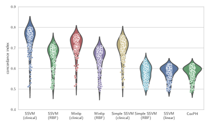
Figure 1: Performance of the proposed ranking-based survival support vector machine compared against other kernel-based survival models and Cox’s proportional hazards model on 100 synthetically generated datasets. In brackets: the kernel function used.

Table 2: Average cross-validation performance on real-world datasets. iAUC: integrated area under the time-dependent, cumulative-dynamic ROC curve.

		SSVM	SSVM	Minlip	SSVM	Cox
		(ours)	(simple)		(linear)
AIDS study	Harrel’s $c$	0.759	0.682	0.729	0.767	0.770
	Uno’s $c$	0.711	0.621	0.560	0.659	0.663
	iAUC	0.759	0.685	0.724	0.766	0.771
Coronary artery disease	Harrel’s $c$	0.739	0.645	0.698	0.706	0.768
	Uno’s $c$	0.780	0.751	0.745	0.730	0.732
	iAUC	0.753	0.641	0.703	0.716	0.777
Framingham offspring	Harrel’s $c$	0.778	0.707	0.786	0.780	0.785
	Uno’s $c$	0.732	0.674	0.724	0.699	0.742
	iAUC	0.827	0.742	0.837	0.829	0.832
Lung cancer	Harrel’s $c$	0.676	0.605	0.719	0.716	0.716
	Uno’s $c$	0.664	0.605	0.716	0.709	0.712
	iAUC	0.740	0.630	0.790	0.783	0.780
WHAS	Harrel’s $c$	0.768	0.724	0.774	0.770	0.770
	Uno’s $c$	0.772	0.730	0.778	0.775	0.773
	iAUC	0.799	0.749	0.801	0.796	0.796

3.2.1 Synthetic Data

The first set of experiments on synthetic data served as a reference on how kernel-based survival models compare to each other in a controlled setup. We performed experiments using an RBF kernel and the clinical kernel [6]. Figure 1 summarises the results on 100 synthetically generated datasets, where all survival times in the test data were uncensored, which leads to unbiased and consistent estimates of the $c$-index. The experiments revealed that using a clinical kernel was advantageous in all experiments (see fig. 1). Using the clinical kernel in combination with any of the SSVM models resulted in a significant improvement over the corresponding model with RBF kernel and linear model, respectively. Regarding the RBF kernel, it improved the performance over a linear model, except for the simple SSVM, which did not perform significantly better than the linear SSVM. The simple SSVM suffers from using a simplified objective function with a restricted set of comparable pairs $\mathcal{P}$, despite using an RBF kernel. This clearly indicates that reducing the size of $\mathcal{P}$ to address the complexity of training a non-linear SSVM, as proposed in [32], is inadequate. Although, the Minlip model is based on the same set of comparable pairs, the change in loss function is able to compensate for that – to some degree. Our proposed optimisation scheme and the Minlip model performed comparably (both for clinical and RBF kernel).

3.2.2 Real Data

In this section, we will present results on 5 real-world datasets (see table 1) based on 5-fold cross-validation and the clinical kernel [6], which is preferred if feature vectors are a mix of continuous and categorical features as demonstrated above. Table 2 summarises our results. In general, performance measures correlated well and results support our conclusions from experiments on synthetic data described above. The simplified SSVM performed poorly: it ranked last in all experiments. In particular, it was outperformed by the linear SSVM, which considers all comparable pairs in $\mathcal{P}$, which is evidence that restricting $\mathcal{P}$ is an unlikely approach to train a non-linear SSVM efficiently. The Minlip model was outperformed by the proposed SSVM on two datasets (AIDS study and coronary artery disease). It only performed better on the veteran’s lung cancer data set and was comparable in the remaining experiments. The linear SSVM achieved comparable performance to the SSVM with clinical kernel on all datasets, except the coronary artery disease data. Finally, Cox’s proportional hazard model often performed very well on the real-world datasets, although it does not model non-linearities explicitly. The performance difference between our SSVM and the Minlip model can be explained when considering that they not only differ in the loss function, but also in the definition of the set $\mathcal{P}$. While our SSVM is able to consider all (valid) pairwise relationships in the training data, the Minlip model only considers a small subset of pairs. This turned out to be problematic when the amount of censoring is high, as it is the case for the AIDS and coronary artery disease studies, which contained less than 15% uncensored records (see table 1). In this setting, training a Minlip model is based on a much smaller set of comparable pairs than what is available to our SSVM, which ultimately leads to a Minlip model that generalises badly. Therefore, our proposed efficient optimisation scheme is preferred both with respect to runtime and predictive performance. When considering all experiments together, statistical analysis [8] suggests that the predictive performance of all five survival models is comparably.

3.3 Conclusion

We proposed an efficient method for training non-linear ranking-based survival support vector machines. Our algorithm is a straightforward extension of our previously proposed training algorithm for linear survival support vector machines. Our optimisation scheme allows analysing datasets of much larger size than previous training algorithms, mostly by reducing the space complexity from $O(n^{4})$ to $O(n^{2})$, and is the preferred choice when learning from survival data with high amounts of right censoring. This opens up the opportunity to build survival models that can utilise large amounts of complex, structured data, such as graphs and strings.

Acknowledgments.

This work has been supported by the CRUK Centre at the Institute of Cancer Research and Royal Marsden (Grant No. C309/A18077), The Heather Beckwith Charitable Settlement, The John L Beckwith Charitable Trust, and the Leibniz Supercomputing Centre (LRZ, www.lrz.de). Data were provided by the Framingham Heart Study of the National Heart Lung and Blood Institute of the National Institutes of Health and Boston University School of Medicine (Contract No. N01-HC-25195).

References

- [1] Bender, R., Augustin, T., Blettner, M.: Generating survival times to simulate Cox proportional hazards models. Stat. Med. 24(11), 1713–1723 (2005)
- [2] Cai, T., Tonini, G., Lin, X.: Kernel machine approach to testing the significance of multiple genetic markers for risk prediction. Biometrics 67(3), 975–986 (2011)
- [3] Chapelle, O.: Training a support vector machine in the primal. Neural Comput. 19(5), 1155–1178 (2007)
- [4] Chapelle, O., Keerthi, S.S.: Efficient algorithms for ranking with SVMs. Information Retrieval 13(3), 201–205 (2009)
- [5] Cox, D.R.: Regression models and life tables. J. R. Stat. Soc. Series B Stat. Methodol. 34, 187–220 (1972)
- [6] Daemen, A., Timmerman, D., Van den Bosch, T., Bottomley, C., Kirk, E., Van Holsbeke, C., Valentin, L., Bourne, T., De Moor, B.: Improved modeling of clinical data with kernel methods. Artif. Intell. Med. 54, 103–114 (2012)
- [7] Dembo, R.S., Steihaug, T.: Truncated newton algorithms for large-scale optimization. Math. Program. 26(2), 190–212 (1983)
- [8] Demšar, J.: Statistical Comparisons of Classifiers over Multiple Data Sets. J. Mach. Learn. Res. 7, 1–30 (2006)
- [9] Doove, L.L., van Buuren, S., Dusseldorp, E.: Recursive partitioning for missing data imputation in the presence of interaction effects. Comput. Stat. Data. Anal. 72(0), 92–104 (2014)
- [10] Eleuteri, A., Taktak, A.F.: Support vector machines for survival regression. In: Computational Intelligence Methods for Bioinformatics and Biostatistics. LNCS, vol. 7548, pp. 176–189. Springer (2012)
- [11] Evers, L., Messow, C.M.: Sparse kernel methods for high-dimensional survival data. Bioinformatics 24(14), 1632–1638 (2008)
- [12] Harrell, F.E., Califf, R.M., Pryor, D.B., Lee, K.L., Rosati, R.A.: Evaluating the yield of medical tests. J. Am. Med. Assoc. 247(18), 2543–2546 (1982)
- [13] Herbrich, R., Graepel, T., Obermayer, K.: Large Margin Rank Boundaries for Ordinal Regression, chap. 7, pp. 115–132. MIT Press, Cambridge, MA (2000)
- [14] Hosmer, D., Lemeshow, S., May, S.: Applied Survival Analysis: Regression Modeling of Time to Event Data. John Wiley & Sons, Inc., Hoboken, NJ (2008)
- [15] Hung, H., Chiang, C.T.: Estimation methods for time-dependent AUC models with survival data. Can. J. Stat. 38(1), 8–26 (2010)
- [16] Kalbfleisch, J.D., Prentice, R.L.: The Statistical Analysis of Failure Time Data. John Wiley & Sons, Inc. (2002)
- [17] Kannel, W.B., Feinleib, M., McNamara, P.M., Garrision, R.J., Castelli, W.P.: An investigation of coronary heart disease in families: The Framingham Offspring Study. Am. J. Epidemiol. 110(3), 281–290 (1979)
- [18] Keerthi, S.S., DeCoste, D.: A modified finite newton method for fast solution of large scale linear SVMs. J. Mach. Learn. Res. 6, 341–361 (2005)
- [19] Khan, F.M., Zubek, V.B.: Support vector regression for censored data (SVRc): A novel tool for survival analysis. In: 8th IEEE International Conference on Data Mining. pp. 863–868 (2008)
- [20] Kimeldorf, G.S., Wahba, G.: A correspondence between Bayesian estimation on stochastic processes and smoothing by splines. Ann. Math. Stat. 41(2), 495–502 (1970)
- [21] Kuo, T.M., Lee, C.P., Lin, C.J.: Large-scale kernel RankSVM. In: SIAM International Conference on Data Mining. pp. 812–820 (2014)
- [22] Lee, C.P., Lin, C.J.: Large-scale linear RankSVM. Neural Comput. 26(4), 781–817 (2014)
- [23] Leslie, C., Eskin, E., Noble, W.S.: The spectrum kernel: A string kernel for SVM protein classification. In: Pac. Symp. Biocomput. pp. 564–575 (2002)
- [24] Li, H., Luan, Y.: Kernel Cox regression models for linking gene expression profiles to censored survival data. In: Pac. Symp. Biocomput. pp. 65–76 (2003)
- [25] Ndrepepa, G., Braun, S., Mehilli, J., Birkmeier, K.A., Byrne, R.A., Ott, I., Hösl, K., Schulz, S., Fusaro, M., Pache, J., Hausleiter, J., Laugwitz, K.L., Massberg, S., Seyfarth, M., Schömig, A., Kastrati, A.: Prognostic value of sensitive troponin T in patients with stable and unstable angina and undetectable conventional troponin. Am. Heart J. 161(1), 68–75 (2011)
- [26] Pölsterl, S., Navab, N., Katouzian, A.: Fast training of support vector machines for survival analysis. In: Machine Learning and Knowledge Discovery in Databases. LNCS, vol. 9285, pp. 243–259. Springer (2015)
- [27] Schölkopf, B., Smola, A., Müller, K.R.: Nonlinear component analysis as a kernel eigenvalue problem. Neural Comput. 10(5), 1299–1319 (1998)
- [28] Shivaswamy, P.K., Chu, W., Jansche, M.: A support vector approach to censored targets. In: 7th IEEE International Conference on Data Mining. pp. 655–660 (2007)
- [29] Uno, H., Cai, T., Pencina, M.J., D’Agostino, R.B., Wei, L.J.: On the C-statistics for evaluating overall adequacy of risk prediction procedures with censored survival data. Stat. Med. 30(10), 1105–1117 (2011)
- [30] Uno, H., Cai, T., Tian, L., Wei, L.J.: Evaluating prediction rules for t-year survivors with censored regression models. J. Am. Stat. Assoc. 102, 527–537 (2007)
- [31] Van Belle, V., Pelckmans, K., Suykens, J.A.K., Van Huffel, S.: Support vector machines for survival analysis. In: 3rd International Conference on Computational Intelligence in Medicine and Healthcare. pp. 1–8 (2007)
- [32] Van Belle, V., Pelckmans, K., Suykens, J.A.K., Van Huffel, S.: Survival SVM: a practical scalable algorithm. In: 16th European Symposium on Artificial Neural Networks. pp. 89–94 (2008)
- [33] Van Belle, V., Pelckmans, K., Suykens, J.A.K., Van Huffel, S.: Learning transformation models for ranking and survival analysis. J. Mach. Learn. Res. 12, 819–862 (2011)
- [34] Van Belle, V., Pelckmans, K., Van Huffel, S., Suykens, J.A.K.: Support vector methods for survival analysis: a comparison between ranking and regression approaches. Artif. Intell. Med. 53(2), 107–118 (2011)
- [35] Vishwanathan, S., Schraudolph, N.N., Kondor, R., Borgwardt, K.M.: Graph kernels. J. Mach. Learn. Res. 11, 1201–42 (2011)
- [36] Zhang, W., Ota, T., Shridhar, V., Chien, J., Wu, B., Kuang, R.: Network-based survival analysis reveals subnetwork signatures for predicting outcomes of ovarian cancer treatment. PLoS Comput. Biol. 9(3), e1002975 (2013)