Time Series Structure Discovery
via Probabilistic Program Synthesis

Abstract

There is a widespread need for techniques that can discover structure from time series data. Recently introduced techniques such as Automatic Bayesian Covariance Discovery (ABCD) provide a way to find structure within a single time series by searching through a space of covariance kernels that is generated using a simple grammar. While ABCD can identify a broad class of temporal patterns, it is difficult to extend and can be brittle in practice. This paper shows how to extend ABCD by formulating it in terms of probabilistic program synthesis. The key technical ideas are to (i) represent models using abstract syntax trees for a domain-specific probabilistic language, and (ii) represent the time series model prior, likelihood, and search strategy using probabilistic programs in a sufficiently expressive language. The final probabilistic program is written in under 70 lines of probabilistic code in Venture. The paper demonstrates an application to time series clustering that involves a non-parametric extension to ABCD, experiments for interpolation and extrapolation on real-world econometric data, and improvements in accuracy over both non-parametric and standard regression baselines.

1 Introduction

Time series data are widespread, but discovering structure within and among time series can be difficult. Recent work by Duvenaud et al. [2] and Lloyd et al. [5] showed that it is possible to learn the structure of Gaussian Process covariance kernels and thereby discover interpretable structure in time series data. This paper shows how to reimplement the ABCD approach from Duvenaud et al. [2] using under 70 lines of probabilistic code in Venture [7]. We formulate structure discovery as a form of “probabilistic program synthesis”. The key idea is to represent probabilistic models using abstract syntax trees (ASTs) for a domain-specific language, and then use probabilistic programs to specify the AST prior, model likelihood, and search strategy over models given observed data.

Several recent projects have applied probabilistic programming techniques to Gaussian process time series. Schaechtle et al. [10] embed GPs into Venture with fully Bayesian learning over a limited class of covariance structures with a heuristic prior. Tong and Choi [11] describe a technique for learning GP covariance structures using a relational variant of ABCD, and then compile the models into Stan [1]. However, probabilistic programming is only used for prediction, not for structure learning or for hyperparameter inference.

The contributions of this paper are as follows. First, we formulate ABCD as probabilistic program synthesis. Second, our implementation supports combinations of gradient-based search for hyperparameters, and Metropolis-Hastings sampling for structure and hyperparameters. Third, we show competitive performance on extrapolation and interpolation tasks from real-world data against several baselines. Fourth, we show that 10 lines of code are sufficient to extend ABCD into a nonparametric Bayesian clustering technique that identifies time series which share covariance structure.

2 Bayesian structure learning as probabilistic program synthesis

Figure 1: Overview of Bayesian structure learning as probabilistic program synthesis.

Figure 2: Executing synthesized model programs to produce Gaussian process datasets. Left: A symbolic structure generated by the AST prior. Center: Equivalent source code of the Venture GP model program, produced by the AST interpreter. Right: Executions of the model program probed with inputs in the region $[0,10]$, which outputs datasets of GP time series.

Our objective in probabilistic program synthesis for Bayesian structure learning is to learn a symbolic representation of a probabilistic model program, by observing outputs of the model program given the inputs at which it was evaluated. The basic idea is to define a joint probabilistic model over (i) the symbolic representation of the program in terms of an abstract syntax tree (AST); (ii) the model program synthesized from the AST; and (iii) data $\mathcal{D}=\{(d^{\textrm{in}}_{i},d^{\textrm{out}}_{i}):i=1,\dots,N\}$ that specifies constraints on observed input-output behavior of $N$ independent executions of the synthesized model program. This framework, summarized in Figure 1, is implemented using:

1. A pair of probabilistic programs, an AST prior and AST interpreter, which together form the synthesis model. The AST prior $\mathcal{G}$ specifies a generative model over ASTs $\mathcal{T}$ for a class of probabilistic model programs, denoted $p_{\mathcal{G}}(\mathcal{T})$. The AST interpreter $\mathcal{I}$ takes as input $\mathcal{T}$ and synthesizes an executable model program $\mathcal{M}$ from it. The interpreter’s distribution over model programs is $p_{\mathcal{I}}(\mathcal{M}|\mathcal{T})$.

2. A synthesized probabilistic model program $\mathcal{M}$, whose structure and hyperparameters are determined by its AST, with a distribution $P_{\mathcal{M}}(d^{\textrm{out}}|d^{\textrm{in}})$ over output data given input data.

3. A probabilistic inference program named the synthesis strategy. Given $N$ input-output data pairs $\mathcal{D}$ generated by an unknown model program $\mathcal{M}$ from the class of programs specified by the synthesis model, it searches over the execution trace of $\mathcal{G}$ to find probable symbolic structures (i.e. ASTs) that explain the data.

Given the description of programs above, the posterior distribution over symbolic structures which the synthesis strategy targets is:

$$P_{\mathcal{G}}(\mathcal{T}|\mathcal{D})\propto p_{\mathcal{G}}(\mathcal{T})\int_{\mathcal{M}}\left(\prod_{i=1}^{n}P_{\mathcal{M}}(d^{\textrm{out}}_{i}|d^{\textrm{in}}_{i})\right)P_{\mathcal{I}}(\mathcal{M}|\mathcal{T})\mathop{}\!\mathrm{d}{\mathcal{M}}.$$ (1)

(a) Synthesis model: AST prior $\mathcal{G}$

⬇

1assume tree_root = () -> {1};

2

3assume get_hyper_prior ~ mem((node_index) -> {

4 // Gradient-safe exponential prior.

5 -log_logistic(log_odds_uniform() #hypers:node_index)

6});

7

8assume choose_primitive = (node) -> {

9 base_kernel ~ categorical(simplex(.2, .2, .2, .2, .2),

10 ["WN", "C", "LIN", "SE", "PER"]) #structure:pair("base_kernel", node);

11 cond(

12 (base_kernel == "WN") (["WN", get_hyper_prior(pair("WN", node))]),

13 (base_kernel == "C") (["C", get_hyper_prior(pair("C", node))]),

14 (base_kernel == "LIN") (["LIN", get_hyper_prior(pair("LIN", node))]),

15 (base_kernel == "SE") (["SE", .01 + get_hyper_prior(pair("SE", node))]),

16 (base_kernel == "PER") (["PER",

17 .01 + get_hyper_prior(pair("PER_l", node)),

18 .01 + get_hyper_prior(pair("PER_t", node))

19 ]))

20};

21

22assume choose_operator = mem((node) -> {

23 operator_symbol ~ categorical(simplex(0.45, 0.45, 0.1),

24 ["+", "*", "CP"]) #structure:pair("operator", node);

25 if (operator_symbol == "CP") {

26 [operator_symbol, get_hyper_prior(pair("CP", node))]

27 } else {

28 operator_symbol

29 }

30});

31

32assume generate_random_program = mem((node) -> {

33 if (flip(.3) #structure:pair("branch", node)) {

34 operator ~ choose_operator(node);

35 [operator, generate_random_program(2 * node), generate_random_program(2 * node + 1)]

36 } else {

37 choose_primitive(node)

38 }

39});

(b) Synthesis model: AST interpreter $\mathcal{I}$

⬇

1assume produce_covariance = (source) -> {

2 cond(

3 (source[0] == "WN") (gp_cov_scale(source[1], gp_cov_bump)),

4 (source[0] == "C") (gp_cov_const(source[1])),

5 (source[0] == "LIN") (gp_cov_linear(source[1])),

6 (source[0] == "SE") (gp_cov_se(source[1]**2)),

7 (source[0] == "PER") (gp_cov_periodic(source[1]**2, source[2])),

8 (source[0] == "+") (

9 gp_cov_sum(produce_covariance(source[1]), produce_covariance(source[2]))),

10 (source[0] == "*") (

11 gp_cov_product(produce_covariance(source[1]), produce_covariance(source[2]))),

12 (source[0][0] == "CP") (

13 gp_cov_cp(source[0][1], .1, produce_covariance(source[1]), produce_covariance(source[2]))))

14};

15

16assume produce_executable = (source) -> {

17 baseline_noise = gp_cov_scale(.1, gp_cov_bump);

18 covariance_kernel = gp_cov_sum(produce_covariance(source), baseline_noise);

19 make_gp(gp_mean_const(0.), covariance_kernel)

20};

(c) Data observation program

⬇

1assume source ~ generate_random_program(tree_root());

2assume gp_executable = produce_executable(source);

3define xs = get_data_xs("./data.csv");

4define ys = get_data_ys("./data.csv");

5observe gp_executable(${xs}) = ys;

(d) Synthesis inference strategy: MH + Gradients

⬇

for_each(arange(T), (_) -> {

infer gradient(

minimal_subproblem(/?hypers), steps=100);

infer resimulate(

minimal_subproblem(one(/?structure)), steps=100)})

Figure 3: Structure discovery in time series via probabilistic program synthesis. Panels 3(a)–3(d) present interacting programs in Venture which correspond to the components in Figure 1.

3 Applying the framework to Bayesian learning of Gaussian process covariance structures

Recent work by Duvenaud et al. [2] and Lloyd et al. [5] showed it is possible to use Gaussian Processes (GPs) to discover covariance structure in univariate time series. In this section, we extend the basic approach from Duvenaud et al. [2] by using probabilistic program synthesis for Bayesian learning over the symbolic structure of GP covariance kernels. The technique is implemented in under 70 lines of Venture code, shown in Figure 3.

We briefly review the Gaussian process, a nonparametric regression technique that learns a function $f:\mathcal{X}\to\mathcal{Y}$. The GP prior can express both simple parametric forms (such as polynomial functions) as well as more complex relationships dictated by periodicity, smoothness, and so on. Following the notation of [9], we formalize a Gaussian process $f\sim\mathrm{GP}(m,k)$ with mean function $m:\mathcal{X}\to\mathcal{Y}$ and covariance function $k:\mathcal{X}\times\mathcal{X}\to\mathbb{R}$ as follows: $f$ is a collection of random variables $\left\{f(x):x\in\mathcal{X}\right\}$, any finite subcollection $[f(x_{1}),\dots,f(x_{n})]$ of which are jointly Gaussian with mean vector $[m(x_{1}),\dots,m(x_{n})]$ and covariance matrix $[k(x_{i},x_{j})]_{1\leq{i,j}\leq{n}}$. The mean $m$ is typically set to zero as it can be absorbed by the covariance. The functional form of the covariance $k$ defines essential features of the unknown function $f$ and so provides the inductive bias which lets the GP (i) fit patterns in data, and (ii) generalize to out-of-sample predictions. Rich GP kernels can be created by composing simple (base) kernels through sum, product, and change-point operators [9, Section 4.2.4].

We now describe the synthesis model (AST prior and AST interpreter), and the class of synthesized model programs for learning GP covariances structures. The AST prior $\mathcal{G}$ (Codebox 3(a)) specifies a prior over binary trees. Each leaf $n$ of $\mathcal{T}$ is a pair $(k_{n},h_{n})$ comprised of a base kernel and its hyperparmaters. The base kernels are: white noise (WN), constant (C), linear (LIN), squared exponential (SE), and periodic (PER). Each base kernels has a set of hyperparameters; for instance, PER has a lengthscale and period, and LIN has an x-intercept. Each internal node $n$ represents a composition operator $o_{n}$, which are: sum ($+$), product ($\times$), and changepoint ($\mathrm{CP}$, whose hyperparameters are the x-location of the change, and decay rate). The structure of $\mathcal{T}$ is encoded by the index $n$ of each internal node (whose left child is $2n$ and right child is $2n+1$) and the operators and base kernels at each node. Let $N=\lvert\mathcal{T}\rvert$ denote the number of nodes. We write $\mathcal{T}=\cup_{n=1}^{N}{\left\{x_{n}\right\}}$ as a collection of $N$ random variables, where $x_{n}=(b_{n},o_{n},k_{n},h_{n})$ is a bundle of random variables for node $n$: $b_{n}$ is 1 if the tree branches at $n$ (and 0 if $n$ is a leaf); $o_{n}$ is the operator (or $\varnothing$ if $b_{n}=0$); $k_{n}$ is the base kernel (or $\varnothing$ if $b_{n}=1$); and $h_{n}$ is the hyperparameter vector (or $\varnothing$ if $n$ has no hyperparameters, e.g., if $b_{n}=1$ and $o_{n}=+$). Letting $\pi(n)$ denote the list of all nodes in the path from $n$ up to the root, the tree prior is:

$$p_{\mathcal{G}}(\mathcal{T}) =\prod_{n=1}^{N}p_{\mathcal{G}}(x_{n}|x_{\pi(n)});$$ (2)

$$=\prod_{n=1}^{N}\begin{cases}(1{-}p_{\mathrm{branch}})\,p_{\mathrm{kernel}}(k_{n})\,p_{\mathrm{hyper}}(h_{n}\,{\mid}\,\mathrm{kernel}=k_{n})&\textrm{if}\;b_{n}=0,\\ (p_{\mathrm{branch}})p_{\mathrm{operator}}(o_{n})p_{\mathrm{hyper}}(h_{n}\,{\mid}\,\mathrm{operator}=o_{n})&\textrm{if}\;b_{n}=1,\\ 0&\textrm{if}\;x_{n}|x_{\pi(n)}\;\textrm{is inconsistent.}\end{cases}$$

The distributions $p_{\textrm{branch}}$, $p_{\textrm{kernel}}$, and $p_{\mathrm{hyper}}$ are all fixed constants in $\mathcal{G}$. An example covariance kernel AST generated by Eq (2) is shown the first column of Figure 2. As for the AST interpreter $\mathcal{I}$ (Codebox 3), it parses $\mathcal{T}$ and deterministically outputs a GP model program with mean 0 and covariance function encoded by $\mathcal{T}$, plus baseline noise. Outcomes of the synthesis step are shown in the second column of Figure 2. The synthesized GP model program $\mathcal{M}$ takes as input $k$ probe points $d^{\textrm{in}}\in\mathbb{R}^{k}$, and produces as output a (noisy) joint sample $d^{\textrm{out}}\in\mathbb{R}^{k}$ of the GP at the probe points:

$$\log P_{\mathcal{M}}(d^{\textrm{out}}|d^{\textrm{in}}) =\log\mathcal{N}(d^{\textrm{out}}\mid 0,\mathbf{K}^{\textrm{cov}}+\sigma^{2}\mathbf{I})\quad\quad(\mathrm{with}\;\mathbf{K}^{\textrm{cov}}=\left[\mathrm{cov}\left(d^{\text{in}}_{a},d^{\text{in}}_{b}\right)\right]_{1\leq a,b\leq k})$$

$$=-\frac{1}{2}(d^{\textrm{out}})^{\top}(\mathbf{K}^{\textrm{cov}}+\sigma^{2}\mathbf{I})^{-1}d^{\textrm{out}}-\frac{1}{2}\log\left\lvert\mathbf{K}^{\textrm{cov}}+\sigma^{2}\mathbf{I}\right\rvert-\frac{k}{2}\log 2\pi.$$

4 Bayesian structure learning and hyperparameter inference in the covariance kernel AST

Our implementation of program synthesis for GP covariances described in the previous section simplifies Eq (1) in that $\mathcal{I}$ deterministically interpreters a GP model program given the AST, so that $P_{\mathcal{I}}(\mathcal{M}|\mathcal{T})=\delta\left[\mathcal{M}=\texttt{interpret}(\mathcal{T};\mathcal{I})\right]$. The key inference problem becomes search over the space of GP kernel compositions in $\mathcal{T}$, and hyperparameters $h_{n}\in\mathcal{T}$ of base kernels. This section describes the synthesis strategy for posterior inference over the AST.

Our strategy for inference on structure is to simulate a Markov chain whose target distribution is $p_{\mathcal{G}}(\mathcal{T}|\mathcal{D})$. The following Metropolis-Hastings algorithm is implemented by the Venture inference program infer resimulate(minimal_subproblem(/?structure)) (invoked in Codebox 3(d)). Suppose the current AST is $\mathcal{T}$. We design a proposal distribution $Q(\mathcal{T}\to\mathcal{T}^{\prime})$ using a three-step process. First, identify a node $x_{n}\in\mathcal{T}$, and let $\mathcal{T}_{n}$ denote the subtree of $\mathcal{T}$ rooted at $n$. Second, “detach” $x_{n}$ and all its descendants from $\mathcal{T}$, which gives an intermediate tree $\mathcal{T}_{\textrm{detach}}:=\mathcal{T}\setminus\mathcal{T}_{n}$. Third, “resimulate”, starting from $\mathcal{T}_{\textrm{detach}}$, the random choice $x^{\prime}_{n}$ using a resimulation distribution $q(x^{\prime}_{n}|\mathcal{T}_{\textrm{detach}})\equiv p_{\mathcal{G}}$ equal to the prior Eq (2). If $b_{n}^{\prime}=0$ (i.e., a branch node), recursively resimulate its children until all downstream random choices are leaf nodes. This operation results in a new subtree $\mathcal{T}^{\prime}_{n}$, and we set $\mathcal{T}^{\prime}=\mathcal{T}_{\textrm{detach}}\cup\mathcal{T}^{\prime}_{n}$ to be the proposal. To compute the reversal $Q(\mathcal{T}^{\prime}\to\mathcal{T})$, we make the following key observation: when resimulating node $x^{\prime}_{n}$ starting from $\mathcal{T}^{\prime}$, the intermediate trees $\mathcal{T}_{\mathrm{detach}}=\mathcal{T}^{\prime}_{\mathrm{detach}}$ are identical for $Q(\mathcal{T}\to\mathcal{T}^{\prime})$ and $Q(\mathcal{T}^{\prime}\to\mathcal{T})$. Using this insight, the MH ratio is therefore:

$$\alpha(\mathcal{T}\to\mathcal{T}^{\prime})=\frac{p_{\mathcal{G}}(\mathcal{T}^{\prime},\mathcal{D})Q(\mathcal{T}^{\prime}\to\mathcal{T})}{p_{\mathcal{G}}(\mathcal{T},\mathcal{D})Q(\mathcal{T}\to\mathcal{T}^{\prime})}=\frac{\left(\prod_{n=1}^{N}p_{\mathcal{G}}(x^{\prime}_{n}|x^{\prime}_{\pi^{\prime}(n)})\right)p_{\mathcal{G}}(\mathcal{D}|\mathcal{T}^{\prime})Q(\mathcal{T}^{\prime}\to\mathcal{T})}{\left(\prod_{n=1}^{N}p_{\mathcal{G}}(x_{n}|x_{\pi(n)})\right)p_{\mathcal{G}}(\mathcal{D}|\mathcal{T})Q(\mathcal{T}\to\mathcal{T}^{\prime})}$$

$$=\frac{\left(\prod_{n\in{\mathcal{T}^{\prime}_{\mathrm{detach}}}}p_{\mathcal{G}}(x^{\prime}_{n}|x^{\prime}_{\pi^{\prime}(n)})\right)\left(\prod_{n\in{\mathcal{T}^{\prime}_{n}}}p_{\mathcal{G}}(x^{\prime}_{n}|x^{\prime}_{\pi^{\prime}(n)})\right)p_{\mathcal{G}}(\mathcal{D}|\mathcal{T}^{\prime})\left(\prod_{n\in{\mathcal{T}_{n}}}p_{\mathcal{G}}(x_{n}|x_{\pi^{\prime}(n)})\right)}{\left(\prod_{n\in{\mathcal{T}_{\mathrm{detach}}}}p_{\mathcal{G}}(x_{n}|x_{\pi(n)})\right)\left(\prod_{n\in{\mathcal{T}_{n}}}p_{\mathcal{G}}(x_{n}|x_{\pi(n)})\right)p_{\mathcal{G}}(\mathcal{D}|\mathcal{T})\left(\prod_{n\in{\mathcal{T}^{\prime}_{n}}}p_{\mathcal{G}}(x^{\prime}_{n}|x_{\pi^{\prime}(n)})\right)}=\frac{p_{\mathcal{G}}(\mathcal{D})\mid\mathcal{T}^{\prime})}{p_{\mathcal{G}}(\mathcal{D}\mid\mathcal{T})}.$$

This likelihood-ratio can be computed without revisiting the entire trace [7]. Algorithm 1 summarizes the key elements of the MH resimulation algorithm described above.

As for hyperparameter inference, Our synthesis strategy uses either MH (for each hyperparameter separately) or gradient ascent (for all hyperparameters jointly). The gradient optimizer uses reverse-mode auto-differentiation [3], propagating gradients down the root of $\mathcal{T}$ to the leaves, and partial derivatives of hyperparameters from leaves back up to the root. Algorithms 2 and 3 describe hyperparameter inference in the AST using MH and gradient-based inference, respectively. All three algorithms are implemented as general purpose inference machinery in Venture.

Algorithm 1 Resimulation MH for the covariance AST.
Inference program: infer resimulate(minimal_subproblem(/?structure==pair("branch", n)))

1:Index $n$ of node in the AST whose subtree structure $\mathcal{T}_{n}$ to transition.

2:MH transition $\mathcal{T}_{n}\to\mathcal{T}_{n}^{\prime}$, targeting $p_{\mathcal{G}}(\mathcal{T}_{n}|\mathcal{T}_{\setminus{n}},\mathcal{D})$.

3:$\mathcal{T}_{\textrm{detach}}\leftarrow\mathcal{T}\setminus\mathcal{T}_{n}$ $\triangleright$ Detach the subtree rooted at $n$.

4:$\mathcal{T}^{\prime}_{n}\sim p_{\mathcal{G}}(\cdot\mid\mathcal{T}_{\textrm{detach}})$ $\triangleright$ Resimulate the subtree rooted at $n$ from the prior.

5:$\mathcal{T}^{\prime}\leftarrow\mathcal{T}_{\textrm{detach}}\cup\mathcal{T}^{\prime}_{n}$ $\triangleright$ Construct the proposal tree.

6:$\alpha\leftarrow p_{\mathcal{G}}(\mathcal{D}\mid\mathcal{T}^{\prime})/p_{\mathcal{G}}(\mathcal{D}\mid\mathcal{T}^{\prime})$ $\triangleright$ Compute the acceptance ratio.

7:if $\textsc{Uniform}[0,1]\leq\alpha$ then $\triangleright$ Accept the proposal with probability $\alpha$.

8:     $\mathcal{T}_{n}\leftarrow\mathcal{T}^{\prime}_{n}$

Algorithm 2 MH transition on hyperparameters of covariance base kernels and operators.
Inference program: infer resimulate(minimal_subproblem(/?hypers==n), steps=T)

1: Index $n$ of node in AST whose hypers to transition; number $T$ of MH steps.

2:MH transition targeting $p_{\mathcal{G}}(h_{n}|\mathcal{D},\mathcal{T}\setminus{\left\{h_{n}\right\}})$.

3:for $t=1,\dots,T$ do

4:     $h^{\prime}_{n}\sim q(\cdot|\mathcal{T},\mathcal{D})$ $\triangleright$ Propose a new value of $h^{\prime}_{n}$.

5:     $q_{\textrm{reverse}}=p(\mathcal{T}\setminus{\left\{h_{n}\right\}},h^{\prime}_{n},\mathcal{D})\,q(h_{n}|(\mathcal{T}\cup{h^{\prime}_{n}})\setminus{\left\{h_{n}\right\}},\mathcal{D})$ $\triangleright$ Compute density of reversal proposal.

6:     $q_{\textrm{forward}}=p(\mathcal{T},\mathcal{D})\,q(h^{\prime}_{n}|\mathcal{T},\mathcal{D})$ $\triangleright$ Compute density of forward proposal.

7:     $\alpha\leftarrow q_{\textrm{reverse}}/q_{\textrm{forward}}$ $\triangleright$ Compute the acceptance ratio.

8:     if $\textsc{Uniform}[0,1]\leq\alpha$ then $\triangleright$ Accept the proposal with probability $\alpha$.

9:         $\mathcal{T}\leftarrow(\mathcal{T}\cup{h^{\prime}_{n}})\setminus{\left\{h_{n}\right\}}$      

Algorithm 3 Reverse auto-differentiation jointly optimizing hyperparameters of all kernels.
Inference program: infer gradient(minimal_subproblem(/?hypers), steps=T, step_size=g)

1:Number $T$ of gradient steps; gradient step size $\gamma$.

2:Gradient ascent on all hypers $\bm{h}=(h_{n}\,{:}\,n\,{\in}\,\mathcal{T})$ optimizing un-normalized posterior $p(\mathcal{D},\bm{h},\mathcal{T}\setminus\left\{\bm{h}\right\})$.

3:$\triangleright$ Posterior factors as $p(\mathcal{D},\bm{h},\mathcal{T}\setminus\left\{\bm{h}\right\})=\mathcal{L}(\bm{h})p(\bm{h}|\mathcal{T}\setminus\left\{\bm{h}\right\})p(\mathcal{T}\setminus\left\{\bm{h}\right\}),$ where $\mathcal{L}(\bm{h})=p(\mathcal{D}|\bm{h},\mathcal{T}\setminus\left\{\bm{h}\right\})$.

4:for $t=1,\dots,T$ do

5:   $(C^{t}_{1},\dots,C^{t}_{n})\leftarrow\textsc{Compute-Covariance-Matrices}(\mathcal{T})$ $\triangleright$ Recompute covariance matrices at all subtrees.

6:   $\mathop{}\!\mathrm{d}{C}^{t}_{1}=\vec{\nabla}\log p(\mathcal{D}|C^{t}_{1})$ $\triangleright$ Compute gradient of $\log\mathcal{L}$ wrt $C^{t}_{1}$.

7:   Backpropagate-Gradient-Subtree$(\mathcal{T},1)$ $\triangleright$ Compute gradients of $\log\mathcal{L}$ wrt $C^{t}_{n}$, $h_{n}$ at all subtrees.

8:   $\mathop{}\!\mathrm{d}{\bm{h}}\leftarrow\mathop{}\!\mathrm{d}{\bm{h}}+\vec{\nabla}\log p(\bm{h}|\mathcal{T}\setminus\left\{\bm{h}\right\})$ $\triangleright$ Add gradient of the prior on $\bm{h}$.

9:   $\bm{h}\leftarrow\bm{h}+\gamma\mathop{}\!\mathrm{d}{\bm{h}}$ $\triangleright$ Jointly update all hyperparameters.

10: AST $\mathcal{T}$; node index $n$; covariance matrix $C^{t}_{n}$ and hyperparameters $h_{n}$ at $\mathcal{T}_{n}$, and at all subtrees

11: Store: gradients $\mathop{}\!\mathrm{d}{C}^{t}_{j}$ and hyperparam partial derivatives $\mathop{}\!\mathrm{d}{h}=\vec{\nabla}_{h_{j,i}}(\log\mathcal{L}(\bm{h}))$ of all children $j$ of $n$.

12:procedure Backpropagate-Gradient-Subtree(AST $\mathcal{T}$, node index $n$)

13:   if $b_{n}\;\mathrm{\bf is}\;1$ then $\triangleright$ A branch node.

14:     if $o_{n}\;\mathrm{\bf is}\;^{\prime}+^{\prime}$ then $\triangleright$ Child gradient is the parent gradient.

15:       $\mathop{}\!\mathrm{d}{C}^{t}_{2n}\leftarrow\mathop{}\!\mathrm{d}{C}^{t}_{n}$ $\triangleright$ Update left child.

16:       $\mathop{}\!\mathrm{d}{C}^{t}_{2n+1}\leftarrow\mathop{}\!\mathrm{d}{C}^{t}_{n}$ $\triangleright$ Update right child.

17:     else $(o_{n}\;\mathrm{\bf is}\;^{\prime}\times^{\prime})$ $\triangleright$ Child gradient is element-wise product of parent gradient and sibling covariance.

18:       $\mathop{}\!\mathrm{d}{C}^{t}_{2n}\leftarrow\mathop{}\!\mathrm{d}{C}^{t}_{n}\odot C^{t}_{2n+1}$ $\triangleright$ Update left child.

19:       $\mathop{}\!\mathrm{d}{C}^{t}_{2n+1}\leftarrow\mathop{}\!\mathrm{d}{C}^{t}_{n}\odot C^{t}_{2n}$ $\triangleright$ Update right child.      

20:     Backpropagate-Gradient-Subtree$(\mathcal{T},2n)$ $\triangleright$ Backpropagate down left subtree.

21:     Backpropagate-Gradient-Subtree$(\mathcal{T},2n+1)$ $\triangleright$ Backpropagate down right subtree.

22:   else $(b_{n}\;\mathrm{\bf is}\;0)$ $\triangleright$ A leaf node.

23:     $\mathop{}\!\mathrm{d}{h}_{n}\leftarrow\mathrm{\bf vec}(\mathop{}\!\mathrm{d}{C}^{t}_{n})\cdot\mathcal{J}_{h_{n}}(K_{n}(\mathcal{D}^{\rm{in}},\mathcal{D}^{\rm{in}}\mid{h_{n}}))$ $\triangleright$ Gradient is product of covariance with kernel’s Jacobian.    

5 Applications to synthetic and real-world datasets

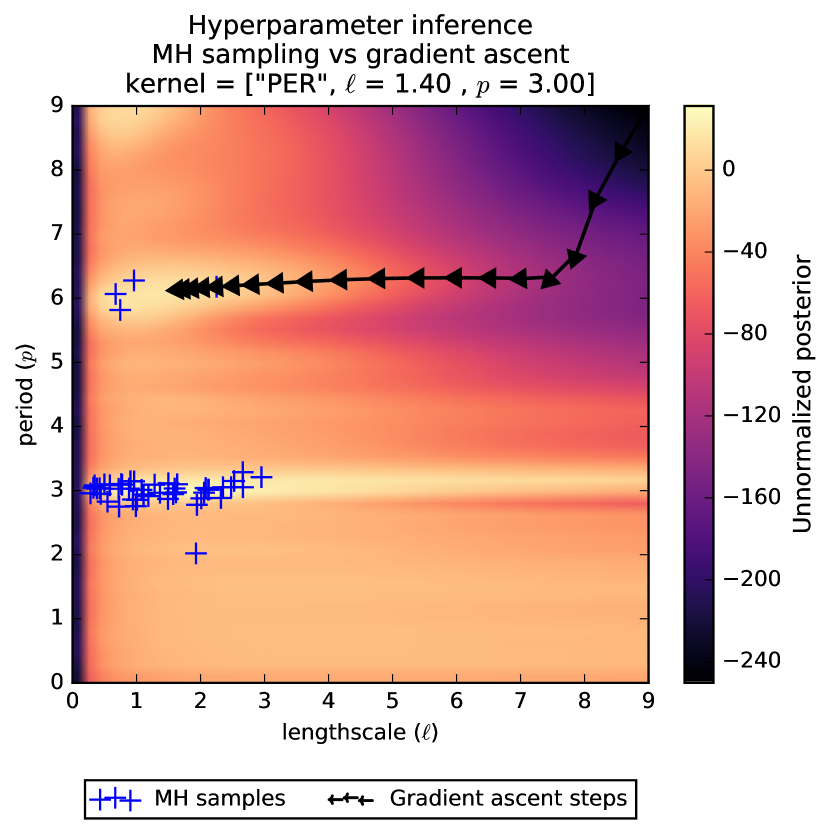
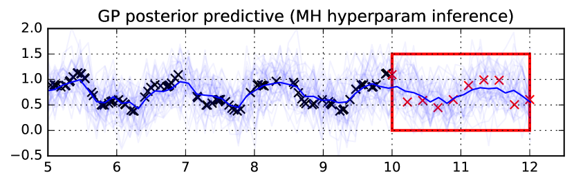
infer resimulate(minimal_subproblem(one(/?hypers)), steps=100) infer gradient(minimal_subproblem(/?hypers), steps=100)

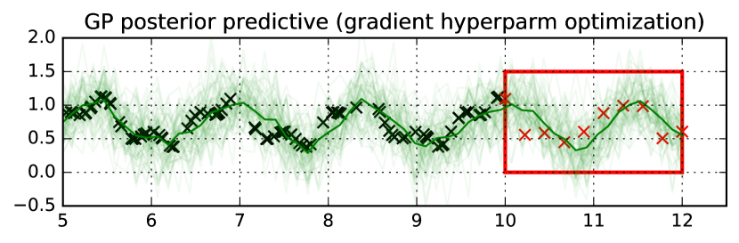
Figure 4: Comparing Metropolis-Hastings sampling and gradient ascent as synthesis strategies for learning GP hyperparameters. The data are drawn from a periodic kernel with length scale 1.4 and period 3. Left: The surface of the unnormalized posterior after observing 200 data points. The gradient ascent steps converge to a local mode at period 6 (a multiple of the true period); the MH sampler explores both posterior modes at periods of 3 and 6. Right: By averaging over modes, posterior predictive curves from the MH inference program (top) illustrate smoother behavior than predictive curves from gradient inference (bottom), which center on a single mode. The mean squared prediction errors on held-out data (red crosses) are 0.18 and 0.20 for MH and gradients, respectively.

 

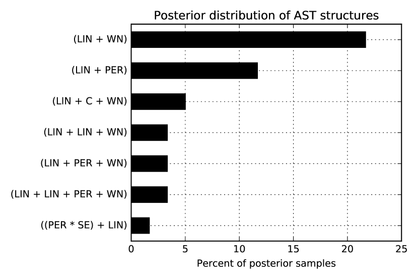
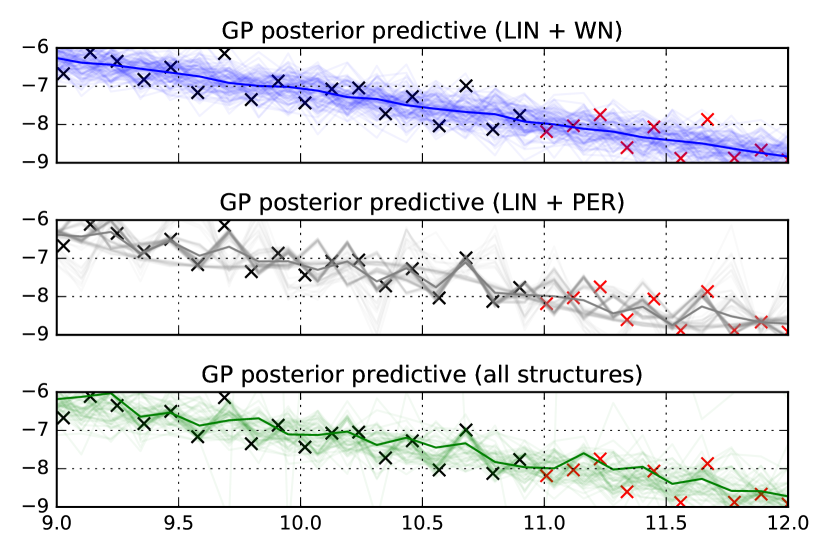
Figure 5: Structure recovery from synthetic data. Left: Histogram of the posterior distribution over AST structures, given data from a LIN + PER Gaussian process. The MAP structure (posterior mode) is LIN + WN. Right: Posterior GP curves sampled from the LIN + WN (blue) and LIN + PER (gray) structures; LIN + PER, which is not the MAP, achieves better predictions on the held-out data (red crosses). Model averaging (green) smooths predictions over all structures.

 

⬇

assume crp = make_crp(0.5);

assume get_cluster_id = mem((ts_index) -> {crp()});

assume get_source = (ts_index) -> {

cluster_id ~ get_cluster_id(integer(ts_index));

generate_random_program(

get_tree_root(), cluster_id)

};

assume obs_function = (ts_index, data) -> {

source = get_source(ts_index);

produce_executable(source)(data)

};

(a) Observation program for clustering GP curves.

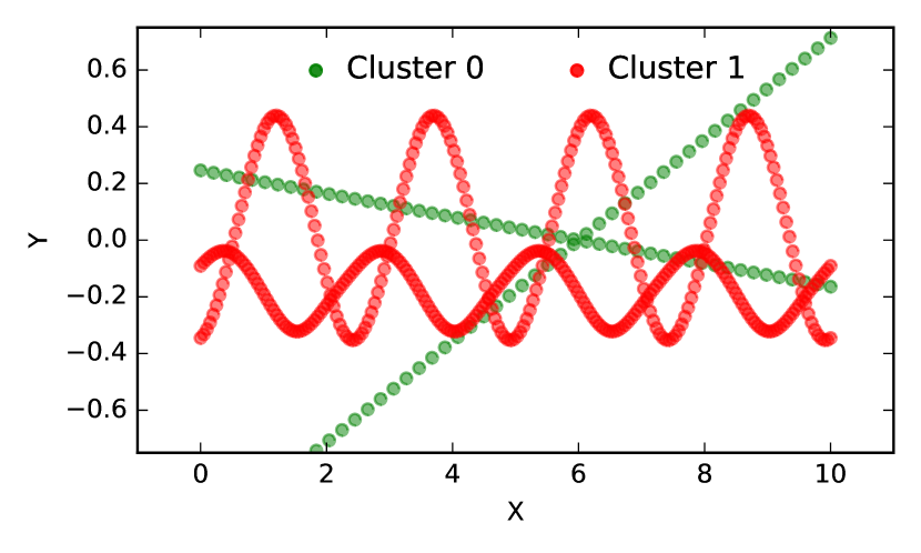
(b) Observed points colored by inferred cluster.

Figure 6: Clustering data according to structural characteristics. Left: A small modification to the model program from Codebox 3(a) suffices to extend it for clustering time series by their covariance structures. Right: Detected clustering among four synthetic time series of 100 points each.

In this section, we apply the probabilistic program synthesis framework for learning GP covariance structures to a collection of synthetic and real-world examples.

The first experiment compares the outcomes of hyperparameter inference using two different inference programs: MH sampling (Algorithm 2) and gradient optimization (Algorithm 3), given data from a periodic GP with period 3 and lengthscale 1.4. By encapsulating inference algorithms as top-level inference programs, it is possible to easily compare both their performance in searching the hyperparameter space, and their predictive outcomes. Refer to the figure caption for further details.

To explore the advantage of Bayesian learning versus greedy search over structures, we ran inference on 50 data points from a GP with a LIN + PER composite covariance kernel. The posterior distribution over structures is shown in Figure 6. The ground truth structure is the second most probable, while the MAP estimate is incorrectly identified as LIN + WN. GP predictives from model averaging over the posterior structure distribution provide a better fit than using the MAP structure.

To assess the flexibility and extensibility of time series discovery as probabilistic program synthesis, we extended the observation program from Codebox 3(c) to specify a non-parametric mixture of several GP curves, as shown in Figure 5(a). We simulated four datasets, (two linear, and two periodic), and then ran joint MH inference over their structures, hyperparameters, and cluster identities. Clusterings based on 64 posterior samples correctly recover the ground-truth partitioning, shown in red and green in Figure 5(b). It is worthwhile to note that this significant change to the probabilistic model is achieved by modifying less than 10 lines of the original code, suggesting it is possible to extend the basic synthesis template from Figure 3 to a variety of time series analysis tasks.

We next applied the technique to regression problems on real-world time series. Figure 8(a) shows extrapolation performance on a dataset of airline passenger volume between 1949 and 1960. The GP detects the linear trend with periodic variation, leading to very accurate predictions. Figure 8(b) shows interpolation on a dataset of solar radiation between the years 1660 and 2010. The GP successfully models the qualitative change at around 1760, which correctly results in different interpolation characteristics at both ends. In contrast, Bayesian linear regression is forced to treat such structural effects as unmodeled noise.

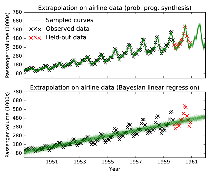
(a) Extrapolation of airline travel volume

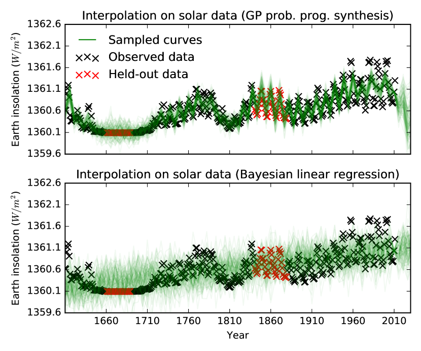
(b) Interpolation of Earth insolation

Figure 8: Comparing GP regression via probabilistic program synthesis and Bayesian linear regression for extrapolating and interpolating on held-out data (red crosses) in real-world time series. The GP learns combinations of periodic and change-point structures, improving predictive performance.

 

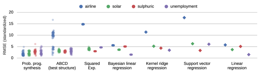
Figure 9: Held-out predictive performance of GP regression via probabilistic program synthesis versus non-parametric regression and standard machine learning baselines on 4 real-world datasets. Each point for the GP methods is the RMSE of a posterior sample, standardized to lowest overall error = 1. The ABCD baseline learns hyperparameters (in Venture) for structures reported by [5].

	Probabilistic program synthesis	ABCD [5]
Main system	69 (Figure 3)	4,166
Gaussian process libraries	2,164 (Venture gpmem [10])	13,945 (GPML Toolbox [8])
Generic inference implementation	1,887 (Venture [7])	—

Figure 10: Lines of code comparison between probabilistic program synthesis in Venture, and ABCD.

Finally, we compared the predictive performance against six baselines on four datasets from Lloyd et al. [5], shown in Figure 10. The GP based on probabilistic program synthesis achieved very competitive prediction error on all tasks. Figure 10 illustrates that implementing probabilistic program synthesis in Venture, an expressive probabilistic programming system with reusable inference machinery, leads to large reductions in code length and complexity.

6 Discussion

We have described and implemented a framework for time series structure discovery using probabilistic program synthesis. We also have assessed efficacy of the approach on synthetic and real-world experiments, and demonstrated improvements in model discovery, extensibility, and predictive accuracy. It seems promising to apply probabilistic program synthesis to several other settings, such as fully-Bayesian search in compositional generative grammars for other model classes [4], or Bayes net structure learning with structured priors [6]. We hope the formalisms in this paper encourage broader use of probabilistic programming techniques to learn symbolic structures in other applied domains.

References

• Carpenter et al. [2017] Bob Carpenter, Andrew Gelman, Matthew Hoffman, Daniel Lee, Ben Goodrich, Michael Betancourt, Marcus Brubaker, Jiqiang Guo, Peter Li, and Allen Riddell. Stan: A probabilistic programming language. Journal of Statistical Software, Articles, 76(1):1–32, 2017.
• Duvenaud et al. [2013] David Duvenaud, James Lloyd, Roger Grosse, Joshua Tenenbaum, and Zoubin Ghahramani. Structure discovery in nonparametric regression through compositional kernel search. In Proceedings of the International Conference on Machine Learning (ICML), pages 1166–1174, 2013.
• Griewank and Walther [2008] Andreas Griewank and Andrea Walther. Evaluating derivatives: principles and techniques of algorithmic differentiation. SIAM, 2008.
• Grosse et al. [2012] Roger Grosse, Ruslan Salakhutdinov, William Freeman, and Joshua Tenenbaum. Exploiting compositionality to explore a large space of model structures. In Proceedings of the Twenty-Eighth Conference Annual Conference on Uncertainty in Artificial Intelligence, pages 306–31, Corvallis, Oregon, 2012. AUAI Press.
• Lloyd et al. [2014] James Lloyd, David Duvenaud, Roger Grosse, Joshua Tenenbaum, and Zoubin Ghahramani. Automatic construction and natural-language description of nonparametric regression models. In AAAI Conference on Artificial Intelligence, pages 1242–1250, 2014.
• Mansinghka et al. [2006] Vikash Mansinghka, Charles Kemp, Thomas Griffiths, and Joshua Tenenbaum. Structured priors for structure learning. In Proceedings of the Twenty-Second Conference Annual Conference on Uncertainty in Artificial Intelligence, pages 324–33, 2006.
• Mansinghka et al. [2014] Vikash Mansinghka, Daniel Selsam, and Yura Perov. Venture: a higher-order probabilistic programming platform with programmable inference. arXiv preprint, arXiv:1404.0099, 2014.
• Rasmussen and Nickisch [2010] Carl Rasmussen and Hannes Nickisch. Gaussian processes for machine learning (gpml) toolbox. Journal of Machine Learning Research, 11(Nov):3011–3015, 2010.
• Rasmussen and Williams [2006] Carl Rasmussen and Christopher Williams. Gaussian Processes for Machine Learning. The MIT Press, 2006.
• Schaechtle et al. [2015] Ulrich Schaechtle, Ben Zinberg, Alexey Radul, Kostas Stathis, and Vikash Mansinghka. Probabilistic programming with Gaussian process memoization. arXiv preprint, arXiv:1512.05665, 2015.
• Tong and Choi [2016] Anh Tong and Jaesik Choi. Automatic generation of probabilistic programming from time series data. arXiv preprint, arXiv:1607.00710, 2016.