The VIMOS Public Extragalactic Redshift Survey (VIPERS).

We use the final catalogue of the VIMOS Public Extragalactic Redshift Survey (VIPERS) to measure the power spectrum of the galaxy distribution at high redshift, presenting results that extend beyond $z=1$ for the first time. We apply a Fast Fourier Transform technique to four independent subvolumes comprising a total of $51,728$ galaxies at $0.6<z<1.1$ (out of the nearly $90,000$ included in the whole survey). We concentrate here on the shape of the direction-averaged power spectrum in redshift space, explaining the level of modelling of redshift-space anisotropies and the anisotropic survey window function that are needed to deduce this in a robust fashion. We then use covariance matrices derived from a large ensemble of mock datasets in order to fit the spectral data. The results are well matched by a standard $\Lambda$CDM model, with density parameter $\Omega_{M}h=\smash{0.227^{+0.063}_{-0.050}}$ and baryon fraction $\smash{f_{B}=\Omega_{B}/\Omega_{M}=0.220^{+0.058}_{-0.072}}$. These inferences from the high-$z$ galaxy distribution are consistent with results from local galaxy surveys, and also with the cosmic microwave background. Thus the $\Lambda$CDM model gives a good match to cosmic structure at all redshifts currently accessible to observational study.

1 Introduction

Present-day large-scale structures are thought to have formed by the gravitational amplification of small initial density perturbations. The galaxies that define the cosmic web are the complicated result of baryonic matter falling into dark-matter potential wells after decoupling, but the overall pattern of inhomogeneity on large scales still largely reflects the initial conditions. If the initial density field, $\delta({\rm\bf x})$, is a Gaussian process, then its statistical properties are completely described by its two-point correlation function, $\xi(r)$, or by its power spectrum, $P(k)$. The shapes of these functions in the linear regime are directly predicted by theory and depend on the key cosmological parameters, especially the total matter density, $\Omega_{M}$, and the baryon fraction, $f_{B}=\Omega_{B}/\Omega_{M}$. There is thus a notable history of using galaxy surveys to probe the primordial fluctuations and thereby learn about the constitution of the Universe.

Any programme for extracting cosmological information from galaxy clustering is complicated by several factors. First, small-scale density perturbations eventually evolve in a non-linear fashion requiring more complex modelling techniques beyond the simple and robust linear-theory predictions. This entails using $N$-body simulations (e.g. Springel et al. 2005) or approximate approaches (e.g. Smith et al. 2003; Bernardeau et al. 2002). Secondly, we only measure the clustering of luminous tracers; but the matter and galaxy fields are connected by a complicated bias relation that may be non-linear, stochastic, and non-local (e.g. Davis et al. 1985; Bardeen et al. 1986; Dekel & Lahav 1999). Thirdly, maps of the large-scale galaxy distribution are built in redshift space: radial peculiar velocities alter the observed redshift, which introduces a preferred direction into the otherwise statistically isotropic clustering pattern (Kaiser 1987).

Significant work has been developed over several decades to overcome these limitations and build galaxy redshift surveys of the ‘local’ ($z<0.1$) Universe capable of obtaining cosmological constraints. These include the Sloan Digital Sky Survey (SDSS: York et al. 2000), in particular through its luminous red galaxy (LRG) extension (Eisenstein et al. 2005), and the Two-degree Field Galaxy Redshift Survey (2dFGRS: Colless et al. 2003). Direct measurements of the power spectrum have been obtained for the 2dFGRS (Percival et al. 2001; Cole et al. 2005a), for the SDSS main galaxy sample (Pope et al. 2004; Tegmark et al. 2004a; Percival et al. 2007), and for the LRGs (Eisenstein et al. 2005; Hütsi 2006; Tegmark et al. 2006; Percival et al. 2007; Beutler et al. 2016). These results provide, together with Supernovae Type Ia and Cosmic Microwave Background (CMB) observations, one of the pillars of the current $\Lambda$CDM cosmological model.

Beyond the lowest-order dependence of the shape of the power spectrum on the overall matter density, there is also a dependence on the contribution of massive neutrinos to the energy budget (e.g. Xia et al. 2012, and references therein) – albeit below current sensitivity if the neutrino masses take the lowest values permitted by oscillation experiments. Beyond this, the baryon fraction is reflected in the presence of finer-scale modulations of the power spectrum: the Baryonic Acoustic Oscillations (BAO), which were first seen and exploited by the 2dFGRS and SDSS (Percival et al. 2001; Cole et al. 2005a; Eisenstein et al. 2005). BAO measurements at different redshifts now provide one of the best probes of the expansion history of the Universe and thus one of the key constraints on the properties of the dark energy that is assumed to drive the accelerated expansion.

Following this path, recent and forthcoming surveys are pushing to higher redshifts, both through a desire to extend the distance scale (Seo & Eisenstein 2007), and also to reduce statistical errors (since cosmic variance declines as sample volume increases). Furthermore, high-$z$ perturbations should be in the linear regime on scales smaller than in the local Universe: $P(k)$ data can then be used up to a larger wave number $k_{\rm{max}}$, thus extracting more information from the observations. The strategy has been in general one of utilising relatively low-density tracers ($\bar{n}\sim 10^{-4}\,h^{3}{\rm Mpc}^{-3}$) to minimise telescope time, exploiting the typical density of fibres achievable with the available fibre-optic spectrographs. This has been the case with the Baryon Oscillation Spectroscopic Survey (BOSS: Dawson et al. 2013), which exploited the SDSS spectrograph further, extending the concept pioneered with the LRGs (e.g. Alam et al. 2016). Similarly, the WiggleZ survey further used the long-lived 2dF positioner on the AAT 4-m telescope, to target UV-selected emission-line galaxies (Drinkwater et al. 2010; Blake et al. 2011a, b).

Covering a large range of redshifts is also of interest through the ability to study the evolution of large-scale structure. Most fundamentally, measurements of the growth of fluctuations through redshift-space distortions (RSD) analysis allow us to discriminate between dark energy models and modifications to Einstein’s theory of gravity (e.g. Guzzo et al. 2008; Zhang et al. 2007; Samushia et al. 2013; Dossett et al. 2015). Also, understanding the simultaneous evolution of structure and galaxy biasing teaches us about both cosmology and galaxy formation, i.e. the complex relationship between dark and baryonic matter. High-density surveys of the general galaxy population (such as 2dFGRS and SDSS Main Galaxy Sample at $z\sim 0.1$) are essential for this task, both to sample the density field adequately and to provide a representative census of galaxy types. This has been the approach of the VIMOS Public Extragalactic Redshift Survey (VIPERS), which currently provides the best combination of volume and spatial sampling for a survey going beyond $z=1$. Its observations were completed recently (January 2016), collecting a final sample of nearly 90,000 redshifts with ${0.5<z<1.5}$. With a high-$z$ volume comparable to that of the 2dFGRS, VIPERS allows us to perform cosmological investigations at $0.6<z<1.1$ with sufficient control of cosmic variance. At the same time VIPERS probes the clustering properties of a broad range of galaxy classes that may be selected by colour, luminosity and stellar mass (Marulli et al. 2013; Granett et al. 2015).

In this paper we estimate the spherically averaged redshift-space galaxy power spectrum $P(k)$ at two different epochs (${0.6<z<0.9}$ and ${0.9<z<1.1}$). We discuss in detail the effects of the survey selection function on the measured power and how these can be accurately accounted for to recover unbiased estimates of cosmological parameters. To this end, we make extensive use of mock catalogues to address the impact of non-linear evolution, bias and the survey mask.

This paper is part of the final set of clustering analyses of the full VIPERS survey, and our intention here is to concentrate on the overall shape of the power spectrum. Redshift-space distortions affect this measurement, but a detailed analysis of the clustering anisotropy and its implications for the growth rate of structures are given in the companion papers: via correlation functions (Pezzotta et al. 2016); in Fourier space with the additional investigation of ‘clipping’ high-density regions (Wilson et al. 2016); and in combination with galaxy-galaxy lensing (de la Torre et al. 2016). In contrast, we focus on the implications of the shape of $P(k)$ for the matter content of the universe, and how our high-$z$ measurements compare with inferences from more local studies. These Large Scale Structures (LSS) focused papers are accompanied by a number of further papers that discuss the evolution of the galaxy population (Cucciati et al. 2016; Gargiulo et al. 2016; Haines et al. 2016).

The paper is structured as follows: in Section 2, we present the real and mock VIPERS data; in Section 3, we describe the methodology for measuring $P(k)$; we discuss our modelling of $P(k)$ in Section 4 and present the results of a likelihood analysis of the VIPERS data in Section 5; in Section 6 we compare our results with analysis performed with previous surveys and summarise our main conclusions in Section 7. Unless explicitly noted otherwise, in our computations of galaxy distances we adopt a cosmology characterised by $\Omega_{M}=0.30$ and $\Omega_{\Lambda}=0.70$.

2 VIPERS

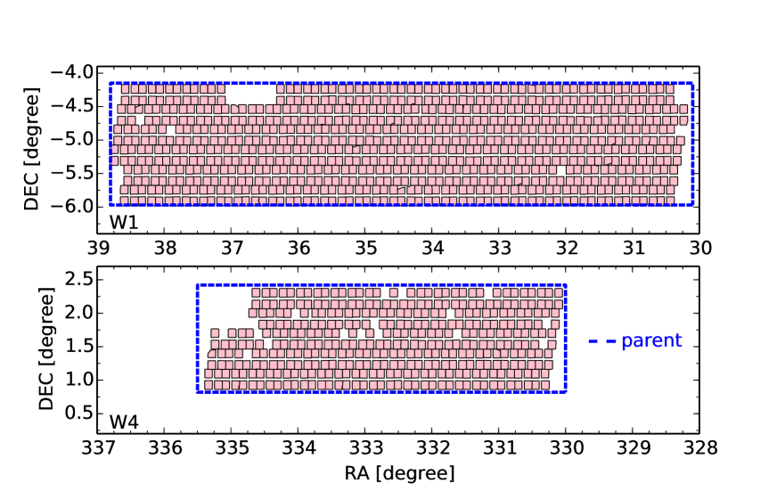
Figure 1: Angular distribution of the full VIPERS galaxy sample, as used for this study (each pink rectangle corresponds to a single quadrant). This shows clearly the geometry and mask produced by the VIMOS footprint. The dashed blue contours define the area of what we call the ‘parent sample’ when we study the survey window function and selection/modelling effects through the use of mock surveys.

The VIMOS Public Extragalactic Redshift Survey (VIPERS: Guzzo et al. 2014; Garilli et al. 2014) has used the VIMOS multi-object spectrograph at the ESO VLT to measure redshifts for a sample of almost $90,000$ galaxies with $i_{\rm AB}<22.5$, over a total area of 23.5 deg². The VIPERS photometric targets were selected from the W1 and W4 fields of the Canada-France-Hawaii Telescope Legacy Survey Wide (CFHTLS, Cuillandre et al. 2012), with an additional pre-selection in colour that robustly removes galaxies with $z<0.5$. Because VIPERS has a single-pass strategy with a maximum target density, the low-$z$ rejection nearly doubles the sampling rate at the high redshifts of prime interest. This yields a mean comoving galaxy density of $\bar{n}\sim 5\times 10^{-3}\,h^{3}\rm{Mpc}^{-3}$ between $z=0.6$ and $z\simeq 1.1$.

The survey area was covered homogeneously with a mosaic of 288 VIMOS pointings (192 in W1, and 96 in W4), whose overall footprint is displayed in Fig. 1. Spectra were taken at moderate resolution ($R=220$) using the LR Red grism, providing a wavelength coverage of 5500-9500 Å. Using a total exposure time of 45 min, this yields an rms redshift measurement error (updated using the final PDR-2 data set) which is well described by a relation $\sigma_{z}=0.00054(1+z)$. For further details on the construction and properties of VIPERS see Guzzo et al. (2014), Garilli et al. (2014) and Scodeggio et al. (2016). This paper is based on the preliminary version of the Second Public Data Release (PDR-2) sample described in the accompanying paper by Scodeggio et al. (2016). The PDR-2 sample includes 340 additional redshifts in the range $0.6<z<1.1$ that were validated after this analysis was at an advanced stage.

The redshift distribution of the final sample is shown in Fig. 2. The solid curve shows the corresponding distribution expected for an unclustered sample. This is derived from the data by convolving the observed weighted distribution (see next section) with a Gaussian kernel with standard deviation $\sigma=100\smash{\,h^{-1}{\rm Mpc}}$. The optimal width of the kernel has been identified by quantifying the impact on the recovered power spectrum from the average of a set of mock samples (see the next section). We have also compared the results with those using alternative ways to reconstruct the expected $\left<N(z)\right>$, as used in other VIPERS papers (e.g. de la Torre et al. 2013), finding no significant differences in the recovered statistics.

As in all VIPERS statistical measurements, we use only galaxies with secure redshift measurements, defined as having a quality flag between 2 and 9 inclusive and corresponding to an overall redshift confirmation rate of $98\%$ (see Guzzo et al. 2014, for definitions).

Figure 2 shows the redshift boundaries of the subsamples defined for this analysis, corresponding to ${0.6<z_{1}<0.9}$ and ${0.9<z_{2}<1.1}$. The lower bound at $z=0.6$ fully excludes the transition region produced by the nominal $z=0.5$ colour-colour cut of VIPERS. In fact, the selection function in this range is well understood, but the gain in volume from adding the $[0.4,0.6]$ slice would be modest. Conversely, the high-redshift limit at $z=1.1$ excludes the most sparse distant part of the survey, where shot noise dominates and so the effective volume is small (Tegmark et al. 2006).

The mean redshifts for the two redshift samples are $\bar{z}_{1}=0.73$ and $\bar{z}_{2}=0.98$. The total numbers of reliable redshifts in each sample, together with their actual and effective volumes (defined following Tegmark et al. 2006) are presented in Table 1. Considering W1 and W4 separately defines four datasets with slightly different window functions. The bias within the two redshift bins will be different due to the different growth factor and the magnitude-limited nature of the survey. Owing to the precise photometric calibration of CFHTLS, the target selection is uniform so that we may adopt the same redshift distribution and bias model for both fields.

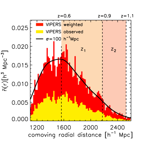
Figure 2: Mean spatial density of galaxies as a function of redshift for the final VIPERS sample used in this analysis. The lower histogram gives the observed distribution, while the top one is obtained after weighting the galaxies with Eq. 1. The solid line gives the estimated mean density distribution, obtained by Gaussian filtering the observed counts with a kernel of $\sigma=100\,h^{-1}\rm{Mpc}$. The vertical dashed lines define the boundaries of the two redshift ranges analysed here.

	W1				W4
$z$-range	$N_{\rm{gal}}$	$V$	$V_{\rm{eff}}$	$z_{\rm{eff}}$	$N_{\rm{gal}}$	$V$	$V_{\rm{eff}}$	$z_{\rm{eff}}$
0.6-0.9	28156	9.8	9.3	0.73	14072	5.3	5.0	0.73
0.9-1.1	6580	8.8	7.4	0.98	2920	4.7	4.0	0.97
‘Full’ VIPERS (0.4-1.2)	48754	27.4	23.5	0.70	24323	14.8	12.7	0.70

Table 1: Number of galaxies and volumes for the four subsamples analysed in this paper, compared to the ‘full’ survey. Volumes are in units of $10^{6}\,h^{-3}\rm{Mpc}^{3}$. Effective volumes are defined following Tegmark et al. (2006), using a reference galaxy power spectrum amplitude of $P_{\rm{eff}}=4000\,h^{-3}\rm{Mpc}^{3}$, as obtained at $k_{\rm{eff}}=0.10\,h\rm{Mpc}^{-1}$.

2.1 Angular masks and incompleteness

The VIPERS angular selection function accounts for the photometric and spectroscopic coverage. Regions around bright stars and with poor photometric quality in CFHTLS have been excluded giving a loss in area of 2.5%. The spectroscopic coverage is determined by the footprint of the VIMOS focal plane and the survey strategy, as seen in Fig. 1. The spectroscopic mask results in a survey filling factor of about $\sim 70\%$. But not all sources in the unmasked area can be targeted for spectroscopy: the slit assignment algorithm (SPOC: Bottini et al. 2005) aims to maximise the number of selected targets with the constraint that spectra may not overlap on the focal plane. On average 47% of targets are assigned a slit in the spectrograph. This completeness fraction defines the target sampling rate (TSR). The result is that close galaxy pairs are missed and the number of spectroscopic targets per quadrant is forced to be approximately constant, independent of the underlying galaxy number density. The effect is not isotropic on the sky, due to the rectangular shape of the spectral footprint. We correct for it as discussed in detail in Pezzotta et al. (2016): we estimate a target sampling rate for each galaxy, ${\rm TSR}_{i}$ within a local region, corresponding to a rectangle with size ${\Delta\rm{RA}\times\Delta\rm{DEC}=60\times 100\,\rm{arcsec^{2}}}$, slightly larger than the 2D VIMOS spectrum. This is a refinement over the technique used in the PDR-1 VIPERS papers (de la Torre et al. 2013), in which an average ${\rm TSR}$ was used on a quadrant-by-quadrant basis.

Once observed, a target may not produce a reliable redshift measurement, depending on the galaxy magnitude, the observing conditions and the available spectral features. The fraction of galaxies with reliable redshifts defines the spectroscopic success rate (SSR), which is $>80$% over the redshift range analysed here. The ${\rm SSR}$ is characterised as a function of galaxy properties and of the VIMOS quadrant, in order to account for varying observing conditions (see Scodeggio et al. 2016).

In addition to the binary photometric/spectroscopic mask, the galaxy selection function is thus given by the product of ${\rm TSR}_{i}$ and ${\rm SSR}_{i}$. While the binary masks are accounted for by the random sample, this selection function is accounted for in the analysis by weighting each galaxy as

$$w_{i}=\frac{1}{{\rm TSR}_{i}\times{\rm SSR}_{i}}\,\,\,\,\,.$$ (1)

We finally note that the colour pre-selection applied to the VIPERS parent photometric sample to isolate galaxies at $z>0.5$ has no effect on this analysis, for two reasons. The Colour Sampling Rate (CSR) (Scodeggio et al. 2016) has in fact been shown to be unity for $z\geq 0.6$; secondly, any residual CSR$(z)$ would not be position-dependent and thus would be absorbed into our model of the redshift distribution.

2.2 Mock catalogues

To test our algorithms and quantify the level of systematic biases in the final estimate of $P(k)$ and to estimate the expected covariance of our measurements, we used a set of mock galaxy samples built to match the properties of the VIPERS survey. These are constructed applying a Halo Occupation Distribution (HOD) prescription to dark-matter haloes from a large $N$-body simulation, calibrating the HOD using the actual VIPERS data. The basic procedure described in de la Torre et al. (2013) and de la Torre et al. (2016) was applied to generate a new set of mocks based on the Big MultiDark $N$-body simulation (BigMD, Klypin et al. (2016)). Thanks to its large volume, we were able to generate 306 and 549 mock catalogues for the W1 and W4 fields respectively. The BigMD assumes a Planck-like cosmology with $(\Omega_{M},\,\Omega_{\Lambda},\,\Omega_{B},\,h,\,n_{s},\,\sigma_{8}\,)$ = (0.307, 0.693, 0.0482, 0.678, 0.960, 0.823).

We define three types of mock samples to be used in our tests: (1) the ‘parent’ mock samples that have the same magnitude and redshift limits as the VIPERS sample, but with no angular selection within rectangular regions enclosing the full W1 and W4 areas (dashed lines in Fig. 1); (2) the ‘mask’ mock samples that exclude galaxies outside the angular mask; and (3) the ‘spectroscopic’ mock samples that further apply the slit-assignment algorithm in the same manner as the real data.

3 Methodology

3.1 Power spectrum estimator

We estimate the galaxy power spectrum using the method by Feldman et al. (1994; FKP). We define the Fourier transform of the density fluctuation field as

$$\delta(\mathbf{k})=\int_{V}\delta(\mathbf{x})\,\exp^{-i\mathbf{k}\cdot\mathbf{x}}\,d^{3}\mathbf{x}\,,$$ (2)

where $V$ is the volume of the galaxy sample. The power spectrum $P(\mathbf{k})$ is then defined by the variance of the Fourier modes:

$$\langle\delta(\mathbf{k})\delta^{*}(\mathbf{k^{\prime}})\rangle=(2\pi)^{3}P(\mathbf{k})\delta_{\rm D}(\mathbf{k}-\mathbf{k^{\prime}})\,\,\,.$$ (3)

The monopole $P(k)$ is then obtained as the spherical average of $P(\mathbf{k})$ for shells in $k$. The practical computation of the monopole involves binning the data on a Cartesian grid and using a Fast Fourier Transform (FFT) algorithm (Jing 2005; Feldman et al. 1994; Frigo & Johnson 2012). The use of the FFT has also been recently suggested as a way to speed-up the computation of higher order multipole moments of the power spectrum (Bianchi et al. 2015; Scoccimarro 2015).

The FFT decomposes the density field into discrete Fourier modes up to the Nyquist frequency $k_{\rm N}=\pi/H$ with spacing $\Delta k=2\pi/L$, where $H$ and $L$ correspond respectively to the distance between two grid points and the total range spanned by the grid. Discretising the signal onto a finite number of cells loses small-scale information leading to aliasing: small-scale fluctuations beyond the Nyquist frequency become translated to larger scales, creating artefacts in the power spectrum. These systematic effects are reduced through the use of a particular mass-assignment scheme (MAS) which applies a low-pass filter.

A common approach corresponds to convolving the galaxy field with a kernel and then sampling at the positions of the grid points (Hockney & Eastwood 1988). We adopt the Cloud-in-Cell (CIC) as MAS with an explicit expression of the window function in configuration space of $W(\mathbf{x})=\prod\limits_{i=1}^{3}W(x_{i}/H)$ , with

$$W(x_{\rm{i}})=\begin{cases}1-|x_{i}|,&\mbox{if }|x_{i}|<1\\ 0,&\mbox{otherwise}\end{cases}$$ (4)

The data are embedded within an FFT cubic grid with side $L=800\,h^{-1}\rm{Mpc}$, and a spacing of $H=2\,h^{-1}\rm{Mpc}$. The corresponding fundamental mode is $k_{\rm{min}}\simeq 0.01\,h\rm{Mpc}^{-1}$, and hence samples minimum wave number of expected fluctuations along the redshift direction in VIPERS. The smallest scale is $k_{\rm{N}}\simeq 1.57\,h\rm{Mpc}^{-1}$.

The normalised density contrast at each point of the FFT grid, $\mathbf{x}_{\rm P}$, is calculated as

$$\hat{\delta}(\mathbf{x}_{\rm{P}})=\,w(\mathbf{x}_{\rm{P}})\,\frac{n_{\rm{G}}(\mathbf{x}_{\rm{P}})-\alpha\,n_{\rm{R}}(\mathbf{x}_{\rm{P}})}{\sqrt{N}}\,.$$ (5)

Here the $G$ and $R$ labels refer to the galaxy and random samples. $n_{\rm R}(\mathbf{x}_{\rm P})$ is the density in a random sample reproducing the full geometry and selection function of the galaxy sample, but with a much higher density than that of the actual galaxies, $n_{\rm G}(\mathbf{x}_{\rm P})$, so that the mean inter-particle separation is much smaller than the cell size, $\lambda\ll H$. Outside the survey volume the overdensity is set to 0. $N$ is defined as

$$N=\int_{\rm{V}}\bar{n}^{2}(\mathbf{x})\,w^{2}(\mathbf{x})\,d^{3}\mathbf{x}=\alpha\sum^{N_{\rm R}}_{i=1}\bar{n}(\mathbf{x}_{i})\,\tilde{w}_{\rm{R}}^{2}(\mathbf{x}_{i})\,,$$ (6)

and represents a normalisation factor that accounts for the radial dependence of the mean density in a magnitude-limited survey. The integral is computed over the total volume of the sample, $V$, and $\alpha$ is the ratio of the effective total number of galaxies $N_{\rm G}$ to the number of unclustered random points $N_{\rm R}$:

$$\alpha=\sum_{i=1}^{N_{\rm{G}}}\tilde{w}_{\rm{G}}(\mathbf{x}_{i})\;/\;\sum_{j=1}^{N_{\rm{R}}}\tilde{w}_{\rm{R}}(\mathbf{x}_{j}).$$ (7)

In these equations $\tilde{w}_{\rm{G}}(\mathbf{x}_{i})$ represents the overall weight assigned to each galaxy:

$${\tilde{w}_{\rm{G}}(\mathbf{x}_{i})=w(\mathbf{x}_{i})\times w_{\rm FKP}(\mathbf{x}_{i})}\,\,;$$ (8)

this combines the survey selection function (Eq. 1) with the FKP weight $w_{\rm FKP}(\mathbf{x})$, designed to minimise the variance of the power spectrum estimator, under the assumption of Gaussian fluctuations:

$$w_{\rm FKP}(\mathbf{x})=\frac{1}{1+\bar{n}(\mathbf{x})P_{\rm{eff}}(k)}\,\,,$$ (9)

We choose $P_{\rm{eff}}=4000\,(h^{-1}\rm{Mpc})^{3}$, corresponding to the amplitude of the VIPERS power spectrum at $k\sim 0.1\,h\rm{Mpc}^{-1}$.

Percival et al. (2004) proposed an extension of the FKP weight to account for the luminosity dependence of bias which in principle can distort the shape of $P(k)$ when estimated from magnitude-limited surveys. The effect arises since distant sources that are more luminous and have a higher bias contribute most to large-scale modes in the power spectrum. We have verified that this issue has no detectable effect on the recovered parameters (see Sect. 5.2).

Each random point is weighted by $\tilde{w}_{\rm R}(\mathbf{x})$ which is equal to the FKP contribution $w_{\rm{FKP}}(\mathbf{x})$.

After Fourier transforming the density field, the monopole power spectrum is obtained by averaging in Fourier shells:

$$\hat{P}(k)=\frac{1}{N_{k}}\sum_{k<|\mathbf{k^{\prime}}|<k+\delta k}|\hat{\delta}(|\mathbf{k^{\prime}}|)|^{2}\;,$$ (10)

This simple estimator is related to the true power by aliasing effects arising from the assignment to a mesh (Jing 2005):

$$\begin{split}\hat{P}(\mathbf{k})=\sum_{\mathbf{n}}|W(\mathbf{k}+2k_{\rm N}\mathbf{n})|^{2}\,P(\mathbf{k}+2k_{\rm N}\mathbf{n})\\ +P_{\rm SN}\sum_{\mathbf{n}}|W(\mathbf{k}+2k_{\rm N}\mathbf{n})|^{2}\;.\end{split}$$ (11)

Here, $\mathbf{n}$ is a vector whose components are any integer; $P_{\rm SN}$ is the Poisson shot-noise contribution due to the discrete sampling of the density field:

$$P_{\rm SN}=\frac{\sum_{i=1}^{N_{\rm G}}\tilde{w}_{\rm G}^{2}(\mathbf{x}_{i})+\alpha^{2}\sum_{j=1}^{N_{\rm R}}\tilde{w}_{\rm R}^{2}(\mathbf{x}_{j})}{N}\,.$$ (12)

The importance of choosing $N_{\rm R}\gg N_{\rm G}$ to minimise contribution to the shot-noise term is evident.

Higher order aliases are damped by the mass assignment window given in Eq. 4; $W(\mathbf{k})$ in Eq. 11 is its Fourier transform:

$$W(\mathbf{k})=\left[\prod\limits_{i=1}^{3}{\rm sinc}{\left(\frac{\pi k_{i}}{2k_{\rm N}}\right)}\right]^{p}.$$ (13)

For the CIC assignment scheme $p=2$ and in this case the aliasing contribution is 1% at $k=0.5k_{\rm N}$ (Sefusatti et al. 2016). To correct for aliasing requires knowledge of the shape of the power spectrum beyond the Nyquist frequency. Jing (2005) proposed an iterative approach; but the speed of the FFT allows us to push $k_{\rm N}$ to very high modes by simply reducing the cell size. For this reason we choose to correct the estimated 3D power spectrum only for the first term ($\mathbf{n}=\mathbf{0}$) in Eq. 11, such that

$$\hat{P}(\mathbf{k})\rightarrow\frac{\hat{P}(\mathbf{k})-S(\mathbf{k})}{W({\mathbf{k}})^{2}}\;.$$ (14)

where $S$ is the shot noise contribution. The aliasing sum arising from the shot noise may be computed analytically in the case when $P_{\rm SN}$ is constant:

$$S(k_{1},k_{2},k_{3})=P_{\rm SN}\times\prod_{i=1}^{3}\left[1-\frac{2}{3}\sin^{2}{\left(\frac{\pi k_{i}}{2k_{\rm N}}\right)}\right]\;.$$ (15)

3.2 Survey window function

The observed galaxy overdensity field arises by a multiplication of the true overdensity by the survey mask: $\delta(\mathbf{x})\rightarrow\delta(\mathbf{x})\times G(\mathbf{x})$. In Fourier space this becomes a convolution of Fourier transforms. Provided the two functions have no phase correlations (fair sample hypothesis), the effect on the power spectrum is also a convolution (Peacock & Nicholson 1991):

$$P_{\rm{obs}}(\mathbf{k})=\int P(\mathbf{k}^{\prime})\,|G(\mathbf{k}-\mathbf{k}^{\prime})|^{2}\,\frac{d^{3}k^{\prime}}{(2\pi)^{3}}\;.$$ (16)

Here, $G(\mathbf{k})$ is the survey window function: the Fourier transform of the mask. We simplify notation by using the same symbol for the mask and its Fourier transform; it should always be clear from context which function is being employed.

In practice, the window must be computed numerically, and we follow the Monte Carlo approach of Feldman et al. (1994), employing dense random catalogues with the same mask and selection function of the VIPERS data, aligning the redshift direction with the $z$ axis. The number density of random objects, $n_{\rm R}(\mathbf{x})$, is assigned to the grid following the same scheme and each point is weighted using Eq. 9. The 3D window function in configuration space at each grid-point position is then given by

$$\hat{G}(\mathbf{x}_{\rm P})=\tilde{w}_{\rm R}(\mathbf{x}_{\rm P})\,\frac{\alpha\,n_{\rm R}(\mathbf{x}_{\rm P})}{\sqrt{N}}\,,$$ (17)

where $N$ is the normalisation factor of Eq. 6. After the Fourier transform, the square modulus of $\hat{G}(\mathbf{k})$ is then corrected for the effects of shot noise and the mass-assignment scheme using Eq. 14.

Figure 3 shows projections along $k_{x},k_{y},k_{z}$ of this estimated window function for the two low-$z$ subsamples. It is important to note the significantly sharper window function along the redshift direction $k_{\rm{z}}$, compared to the other two axes. It should also be noted how the double extension in right ascension of the W1 field with respect to the W4 one already sharpens the corresponding $|G(k_{\rm{y}})|^{2}$. The effects of the overall geometry (dashed line) and of the survey mask (solid line) are also evident. We note in particular how the small-scale gaps in the VIMOS footprint (see Fig. 1) are reflected in the broad wing features emerging at $k>0.5$.

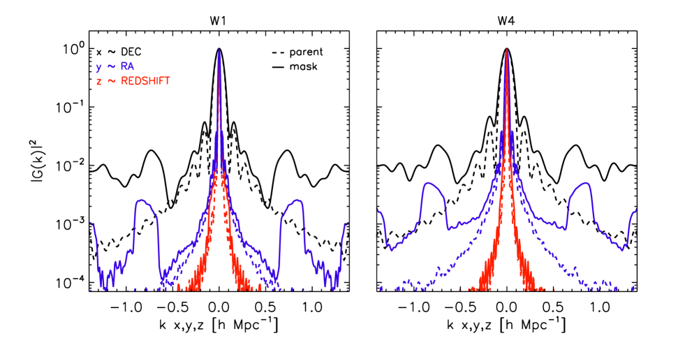
Figure 3: Survey window functions for the W1 and W4 samples at $0.6<z<0.9$, projected along the $k_{x}$, $k_{y}$, $k_{z}$ directions; the dashed lines correspond to considering only the geometry of the parent sample, while the solid lines give the final window function, when the small-scale angular features of the mask are included. The two samples at $0.9<z<1.1$ show approximately similar window functions.

3.3 Accounting for the Window Function

In principle, the window could be deconvolved from the measured power spectrum. But the reconstruction can never be perfect, so the errors are complicated to understand. In contrast, errors of the raw empirical power spectrum are relatively simple, as discussed by FKP, and the forward modelling of convolving a theoretical power spectrum is in principle exact. We therefore follow this commonly adopted route.

If the power spectrum was isotropic, the 3D integral in Eq. 16 can be computed over the spherically averaged window. However, this symmetry is broken in redshift space: owing to the anisotropy introduced by RSD, we must perform the 3D integral first and then spherically average the result. An analytic approximation to obtain the multipoles of $P(\mathbf{k})$ in this case has been proposed by Wilson et al. (2015).

The fastest way of calculating the required convolution is, as usual, to employ the Fast Fourier Transform (FFT). This means that in fact we transform the product of the model correlation function and the transform of the squared window, where the correlation function itself is the transform of the model power:

$$\begin{split}P_{\rm{conv}}(\mathbf{k})={\rm FFT}^{-1}\,{\rm FFT}\,\big{[}G^{2}\otimes P_{\rm M}\big{]}=\\ {\rm FFT}^{-1}\,\big{[}{\rm FFT}\,G^{2}\times{\rm FFT}\,P_{\rm M}\big{]}\;.\end{split}$$ (18)

Here, $P_{\rm M}$ is the theoretical model and $P_{\rm{conv}}$ the convolved power spectrum that should be compared with the measured one. This is the approach of Sato et al. (2011); its only potential deficiency is that memory limitations may prevent the FFT mesh reaching to sufficiently high wave numbers.

Finally, the integral constraint ($IC$) term needs to be subtracted from $P_{\rm{conv}}(k)$ to reflect the fact that the mean density is estimated from the survey volume itself. The power must thus vanish at $k=0$, requiring (Peacock & Nicholson 1991; Percival et al. 2007)

$$IC=\frac{|G(\mathbf{k})|^{2}}{|G(0)|^{2}}\int P(\mathbf{k})\,|G(\mathbf{k})|^{2}\,\frac{d^{3}k}{(2\pi)^{3}}\;.$$ (19)

We test the accuracy of this procedure using our set of mocks. We run CAMB (Lewis & Challinor 2011) with the same cosmological parameters of the BigMD, including the HALOFIT by Smith et al. (2003) (which has been updated by Takahashi et al. (2012)) to model non-linearities, to obtain the reference power spectrum that has to be convolved. In doing this, galaxy bias is left as a free parameter, an assumption that will be justified for VIPERS in Sect. 4.

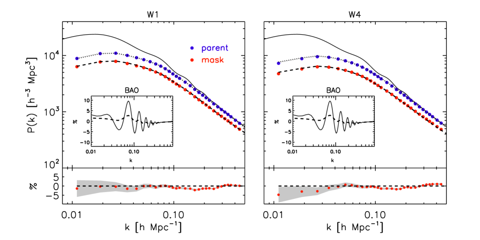
Figure 4: Modelling the effects of the survey window function. The effects of the simplified geometry of the survey only, i.e. the parent sample (filled blue circles) and of the full angular mask (filled red circles) are compared. The dashed and dotted lines show how well these effects are modelled by convolving the input $P(k)$ (solid line) with our model for the window functions of the two cases. The relative accuracy in the case of the full window function (geometry plus mask) is explicitly shown in the bottom panel. The insets show a blow-up of the Baryonic Acoustic Oscillations, obtained by dividing the input spectrum by a “no-wiggles” one (solid line). This is compared to the actual signal expected when $P(k)$ is convolved with the VIPERS window function (dashed line).

Figure 4 shows the results of this test, comparing the convolved model with the average measurements from the ‘observed’ mock samples for the two fields W1 and W4 in the $0.6<z<0.9$ range. We also distinguish the cases when only the parent survey geometry is applied to the mocks and when the full angular mask is included. Both of these results are compared with the model prediction, after re-scaling for the bias value and convolution with the appropriate window function. The bottom panels show residuals, indicating that our modelling can match the mock results with errors no larger than 1–2% – which is as good as perfect for the present application.

The same figure also shows the dramatic impact of the VIPERS window function on the amplitude of the Baryonic Acoustic Oscillations. Nevertheless, as shown in the following section, the overall shape of the power spectrum preserves information on the baryon fraction and other cosmological parameters, once the window function is properly accounted for.

4 Modelling the galaxy power spectrum

4.1 Non-linearity, biasing and redshift-space distortions

The measured $P({\bf k})$ is modified by three main effects that need to be taken into account in the modelling: (a) non-linear evolution of clustering, (b) redshift-space distortions and (c) galaxy bias.

In practice, the effect of non-linear evolution is mitigated by using large-scale data below a given $k_{\rm{max}}$, while at the same time adopting an analytical prescription to account for the residual non-linear deformation of $P(k)$ (Smith et al. 2003; Takahashi et al. 2012). Over the same range of quasi-linear scales we also assume that galaxy bias can be treated as a simple scale-independent factor that multiplies the non-linear matter $P(k)$. This is consistent with previous studies of the bias scaling and non-linearity in VIPERS (Marulli et al. 2013; Di Porto et al. 2014; Cappi et al. 2015; Granett et al. 2015). Moreover the analysis of the mock catalogues in Sect. 3.3 confirms that a constant bias factor is sufficient given that the adopted galaxy formation model is accurate.

Finally, the measured redshifts are affected by peculiar velocities. The present analysis is not concerned with the main resulting effect, which is an induced anisotropy of the power spectrum, but redshift-space distortions will still alter the spherically averaged power. The linear RSD effect was analysed by Kaiser (1987), who showed that coherent velocities streaming from underdensities onto overdensities would introduce a quadrupole anisotropy in the measured power. This in itself does not change the shape of the spherically-averaged power: rather, the amplitude is boosted by a scale-independent factor. But on non-linear scales, comparable to groups and clusters, galaxies inside virialised structures have random peculiar velocities. These produce ‘Finger-of-God’ (FoG) radial smearing that systematically damps modes where the wave vector runs nearly radially (e.g. Peacock & Dodds 1994) – and this effect reduces high-$k$ power even after averaging over directions. Thus, an RSD model is required for the present analysis, and we employ the simple dispersion model (Peacock & Dodds 1994), in which the Kaiser (1987) anisotropy is supplemented by an exponential damping to represent FoG damping:

$$P_{\rm s}(\mathbf{k})=b^{2}\,P_{\rm r}(\mathbf{k})\,(1+\beta\mu_{\mathbf{k}}^{2})^{2}\,e^{-(\sigma_{\rm{TOT}}\,k\,\mu)^{2}}\,,$$ (20)

where $P_{\rm s}$ is the redshift-space power spectrum; $\beta=f/b$, where $f$ is the logarithmic growth rate of structure ($f\approx\Omega_{M}^{\gamma}(a)$, where $\gamma=0.55$ for standard gravity); $\sigma_{\rm{TOT}}$ is in units of ($h^{-1}\rm{Mpc}$) and includes the effects of both the velocity dispersion of galaxy pairs $\sigma_{v}(1+z)/H(z)$ and the VIPERS rms redshift error (see below); $\mu_{\@vec{k}}$ is the cosine of the angle between $\mathbf{k}$ and the line-of-sight, which in the FFT grid coincides with the $z$-direction so as to comply with the plane-parallel approximation.

Given the anisotropy of the VIPERS window function (see Fig. 3), RSD should be included in the 3D model $P_{\rm s}(\mathbf{k})$ before convolving with the window as discussed in Sect. 3.3. This issue was ignored in past work where the window was more isotropic (e.g. Cole et al. 2005a), but our tests on mock data show that it is important for VIPERS: simply convolving the model monopole power spectrum with the 3D window function yields a poor agreement with the monopole power taken directly from the mocks. In contrast, the full 3D modelling method matches the mock monopole power to a tolerance of just a few percent on the scales used in our analysis.

As mentioned above, the effect of the VIPERS redshift measurement errors is considered as an rms contribution within the RSD Gaussian damping term, as estimated directly from the data: $\sigma_{z}=0.00054(1+z)$ or $\sigma_{cz}=162(1+z)\,\rm{km\,s^{-1}}$ (Scodeggio et al. 2016). $\sigma_{cz}$ is of the order of the dispersion of galaxy peculiar velocity, $\sigma_{v}$. The two contributions can be added in quadrature, to produce an ‘effective’ pairwise correction to be used in the power spectrum damping factor: $\sigma_{\rm{TOT}}=(\sigma_{v}^{2}+\sigma_{cz}^{2}(1+z)^{-2})^{1/2}$. This choice has been tested and verified on the mocks.

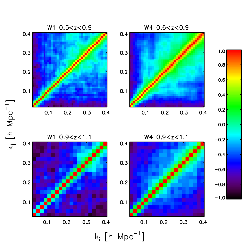
Figure 5: Estimates of the correlation matrices for the four VIPERS subsamples analysed here, constructed using the BigMD mock catalogues as described in Sect. 5.1. It should be noted that the binning is different in the low- and high-redshift samples. Non-Gaussian contributions to the covariance matrix on small scales have greater importance at low redshift.

4.2 Projection effects

The conversion of observed angular coordinates and redshifts into comoving positions introduces an additional dependence on the cosmological model (Alcock & Paczynski 1979). Formally the coordinates must be recomputed for each point in the model parameter space; however, the effort can be avoided by using the method introduced by Ballinger et al. (1996) that we follow here. The following scaling parameters are introduced to express the conservation of the redshift and angular separation of galaxy pairs, $\Delta z$ and $\Delta\theta$:

$$\alpha=(\alpha_{\perp}^{2}\alpha_{\parallel})^{\frac{1}{3}}\;.$$ (21)

Here

$$\alpha_{\perp}=\frac{D_{A,\rm{model}}}{D_{A,\rm{fiducial}}}\;,$$ (22)

where $D_{A}$ is the angular comoving distance, and

$$\alpha_{\parallel}=\frac{H_{\rm{fiducial}}(\bar{z})}{H_{\rm{model}}(\bar{z})}\;,$$ (23)

where $H(\bar{z})$ is the Hubble rate at the mean redshift $\bar{z}$ of the sample.

In the case of a compact survey with fairly isotropic window function, $1/\alpha$ can be used directly to re-scale pair separations $r$ when computing the galaxy correlation function. In the case of $P(k)$, we need to rescale wave numbers as follows:

$$\begin{cases}k_{\rm{x,fiducial}}&=\;k_{\rm{x,model}}\times\alpha_{\perp}\\ k_{\rm{y,fiducial}}&=\;k_{\rm{y,model}}\times\alpha_{\perp}\\ k_{\rm{z,fiducial}}&=\;k_{\rm{z,model}}\times\alpha_{\parallel}\;,\end{cases}$$ (24)

and also multiply the power by $\rm{1/\alpha^{3}}$. This must be done before the convolution with the anisotropic window function.

5 Likelihood Analysis

5.1 Covariance matrix

We now have in hand all the ingredients needed in order to infer cosmological parameters from the measured clustering power spectrum in VIPERS. However, in order to compute the likelihood of the data for a given model, we need to know the covariance matrix between the power in different modes – which in general has a complicated non-diagonal structure. This is easily computed if we have a number of independent realisations of the power spectrum (e.g. from mock data). The estimator for the covariance between the $i$ and $j$ power bins is

$$C_{ij}=\frac{1}{N_{\rm{r}}-1}\sum_{m=0}^{N_{r}}\big{[}P_{\rm m}(k_{i})-\bar{P}(k_{i})\big{]}\big{[}P_{\rm{m}}(k_{j})-\bar{P}(k_{j})\big{]}\;,$$ (25)

where $P_{\rm m}(k)$ is one of $N_{\rm r}$ independent estimates of the power spectrum and $\bar{P}(k)$ is the mean. For a number of bins $N_{\rm{b}}\sim 40$, a few hundred mocks is required in order to obtain a precise covariance matrix (Percival et al. 2014). The BigMD mocks described in Sect. 2.2 fulfil this need. An unbiased estimate of the inverse covariance matrix is then given by (Percival et al. 2014)

$$\Psi_{ij}=(1-D)\;C^{-1}_{ij},\,\,D=\frac{N_{\rm{b}}+1}{N_{\rm{r}}-1}\,\,\,.$$ (26)

The covariance is approximately diagonal as would be expected for a Gaussian random field although coupling between modes is evident. On large scales the dominant effect is due to the window function (Sect. 3.3). On small scales the processes of structure formation produce non-Gaussian correlations that are indeed more evident in the low-redshift bin.

5.2 Overall Consistency test

Before turning to real data, we need to perform an overall test of the modelling pipeline: at which level can our analysis recover an unbiased estimate of the input cosmology of the mock samples, given realistic errors?

To this end, we have constructed a precise estimate of the monopole power spectrum in two redshift ranges, $0.6<z<0.9$ and $0.9<z<1.1$, by averaging respectively the $306$ (for W1) and $549$ (for W4) measurements of the corresponding BigMD mocks. Results are shown here for the low-redshift bin, where non-linearities are expected to be more severe, but we also checked that the same conclusions are valid in the high-redshift sample. The two ‘super-estimates’ for W1 and W4 have then been combined in a single likelihood with the models, as we do for the data. Since the volume of W1 is essentially twice that of W4, this is overall equivalent – in terms of volume – to a measurement performed over $(306\times 2+549)/3=387$ quasi-independent VIPERS surveys. This leads to an expected reduction of the statistical errors by a factor $\smash{\sqrt{387}}\simeq 20$), but the measurement will be characterised by the same window function and non-linear effects that we have modelled in the previous sections.

We have obtained theoretical power spectra $P_{M}(k)$ using CAMB, using the HALOFIT option to give an approximate model of non-linear evolution. The matter density parameter $\Omega_{M}$, the baryon fraction $f_{B}$, the Hubble parameter $h$ and the bias $b$ are left free, while all remaining cosmological parameters are fixed to the values used in the BigMD simulation. Each model power spectrum is derived at our empirical mean redshift, $\bar{z}=0.73$. We then evaluate the VIPERS window function separately for the W1 and W4 fields and perform the 3D convolution using the redshift-space model of Eq. 20; in this expression, the velocity dispersion $\sigma_{v}$, with the inclusion of Gaussian redshift errors, has been estimated thanks to previous tests where $\Omega_{M}$ was fixed to the true value. Finally, we subtract the integral constraint.

The likelihood between the measurements and the model is then computed accounting for the inverse covariance matrix as estimated above

$$\chi^{2}(\mathbf{p})\equiv\sum_{ij}\big{[}P(k_{i})-P_{\rm{M}}(k_{i},\mathbf{p})\big{]}\,\Psi_{ij}\,\big{[}P(k_{j})-P_{\rm M}(k_{j},\mathbf{p})\big{]}\;,$$ (27)

where $\mathbf{p}=\{\Omega_{M},f_{B},h,b,\sigma_{v}\}$ is the parameter vector. On four parameters we set flat priors: $\Omega_{M}$ ($0.2<\;\Omega_{M}<0.4$), $f_{B}$ ($0<\;f_{B}<0.3$), Hubble parameter ($0.6<\;h<0.8$), bias $(1<\;b<2\;$), while for the velocity dispersion we assume a Gaussian prior with a dispersion of $\pm 12\;\rm{km\,s^{-1}}$ consistent with VIPERS data (see below). We consider a restricted range of wave number, $0.01<k<k_{\rm{max}}$, estimated in bins spaced by $\Delta k=0.01\smash{\,h\,{\rm Mpc}^{-1}}$. The minimum value of $k$ corresponds to the maximum extent of the sample in the redshift direction; the choice of $k_{\rm{max}}$ has a more critical impact on the precision and accuracy of the parameter estimates. Statistical errors on $P(k)$ are small on smaller scales, but non-linearities may not be properly modelled if we set $k_{\rm{max}}$ too high.

In Fig. 6, we test this effect by progressively increasing $k_{\rm{max}}$ and showing the impact on the $\chi^{2}$ contours in the $(\Omega_{M}h,f_{B})$ plane for the simulated combined W1 and W4 fields. We see that using a maximum wave number $k_{\rm{max}}=0.40\,h\rm{Mpc}^{-1}$ (i.e. including $N_{\rm b}=40$ bins in the fit) we are still able to properly describe non-linearities, while excluding significant effects from non-linear bias and slit-exclusion effects. The values $\Omega_{M}h\simeq 0.208$ and $f_{B}\simeq 0.157$ of the BigMD are well recovered even compared to the tiny statistical uncertainty of the ‘super-mock-sample’ used for the test. In the case of the real VIPERS measurements, the statistical errors will be a factor of $\smash{\sim\sqrt{387}}$ larger, indicating that the overall systematic biases in our methodology should be at least an order of magnitude smaller than the error bars.

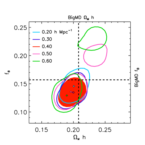
Figure 6: Mean power spectrum from the set of VIPERS mocks used to test the systematic accuracy of the model in recovering the cosmological parameters when including progressively smaller scales. The cosmology of the simulation is indicated by the horizontal and vertical reference lines, and the coloured lines show 68% confidence levels for different values of $k_{\rm max}$. We find no indication of systematic bias when using scales up to $k_{\rm max}=0.40\smash{\,h\,{\rm Mpc}^{-1}}$. Using $k_{\rm max}\geq 0.50\smash{\,h\,{\rm Mpc}^{-1}}$ we find a degeneracy in the constraints. We select $k_{\rm max}=0.40\smash{\,h\,{\rm Mpc}^{-1}}$ for our standard analysis indicated by the filled contour.

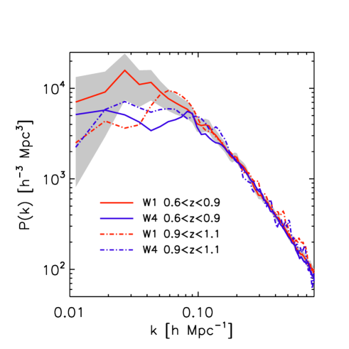
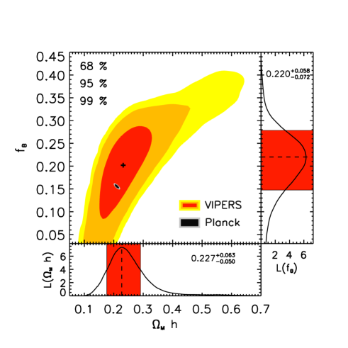
Figure 7: Left: estimates of the monopole of the redshift-space power spectrum from the four independent VIPERS subsamples in W1 and W4 and two redshift bins. The shaded area gives the diagonal error corridor around the $0.6<z<0.9$ W1 sample, as provided by the dispersion of the corresponding mock catalogues. Right: corresponding likelihood surfaces for the simultaneous fit to the four power spectra. The contours correspond to two-parameter confidence levels of 68, 95 and 99 per cent. The measurements have been used down to scales corresponding to $k_{\rm{max}}=0.40\smash{\,h\,{\rm Mpc}^{-1}}$ and we have marginalised over the galaxy bias and velocity dispersion.

6 Results

6.1 The VIPERS galaxy power spectrum

We now apply the machinery developed and tested in the previous sections. Figure 7 shows the estimated power spectra from the four subsamples of the full VIPERS data defined in Sect. 2. The grey area indicates the $1-\sigma$ error corridor (for one sample only, for clarity; it is similar for all samples). Errors correspond to the square root of diagonal elements of the covariance matrix, $\sqrt{C_{\rm{ii}}}$. The contribution of the shot-noise term is ${P_{\rm SN}\simeq 250\;h^{-3}\rm{Mpc}^{3}}$ for the two low redshift bins and ${P_{\rm SN}\simeq 800\;h^{-3}\rm{Mpc}^{3}}$, in the high-redshift range (due to the sparser galaxy density). We have tested with mock samples that the different effects of the four window functions on the overall shape are significant at $k<0.02\smash{\,h\,{\rm Mpc}^{-1}}$, but all four estimates are statistically consistent in this regime – thus cosmic variance dominates over any differences in the windows.

The consistency between the high- and low-redshift samples further confirms that the linear biasing and redshfit-space distortion model is adequate over the full redshift range. This would not necessarily be true if the high-redshift sample suffers from incompleteness which could introduce a scale dependence in the bias. Any such effect was expected to be small, given the stability of the estimated spectroscopic success rate as a function of redshift and spectral type, at least up to $z=1$ (left panel in Fig.7 of Scodeggio et al. 2016); nevertheless, the observed consistency in the spectral shape between the two redshift ranges, especially over the scales used in the likelihood analysis, confirms this. Performing the likelihood analysis in the two redshift samples separately, we obtain fully consistent values for the matter density ${\Omega_{M}h}$ and the baryon fraction $f_{B}$ within the error bars. On the basis of this, we feel even more confident that the power spectra from the two bins can be safely combined into a single likelihood to obtain the VIPERS reference estimates, as we do in the next section.

6.2 Constraints on the matter density parameter and the baryon fraction

Following Percival et al. (2001), Cole et al. (2005a) and Blake et al. (2010), we now investigate the constraints that our results can place on the values of the matter density ${\Omega_{M}h}$ and the baryon fraction $f_{B}$. The density is mainly constrained through the combination ${\Omega_{M}}h$, which fixes the wave number corresponding to the horizon size at matter-radiation equality $k_{\rm{eq}}$, while the baryon fraction is measured through the amplitude of the BAO oscillations (the fact that these are small gives very direct evidence that the Universe is dominated by collisionless matter). Both these aspects are tightly constrained by the CMB, of course, but for clarity it is interesting to see what information is given by LSS alone. However, our analysis cannot be made entirely CMB-free, since there is a degeneracy with the spectral tilt that is hard to break. Cole et al. (2005a) showed that the best-fitting value of $\Omega_{M}h$ from the 2dFGRS reduced linearly with increasing $n_{s}$, with a coefficient of 0.3, and we expect a similar coefficient here. We adopt as exact the value $n_{s}=0.9677$ (Planck Collaboration et al. 2015), so that $\Omega_{M}h$ is raised by 0.010 from the value that would have been obtained on the assumption of scale-invariant primordial fluctuations.

For other parameters, we adopt relatively broad priors and checked that our marginalised results are not sensitive to the prior range. Unless otherwise noted, we assume a flat $\Lambda$CDM Universe with flat priors on $f_{B}$ $(0<f_{B}<0.5)$, $\Omega_{M}$ $(0.1<\Omega_{M}<0.9)$, bias $(1<b<2)$ and the Hubble parameter $(0.6<h<0.8)$. The range of bias explored contains the estimates made in previous VIPERS analyses but is large enough to be non-informative, even for the high-redshift bin (Marulli et al. 2013; Di Porto et al. 2014; Cappi et al. 2015). For the dispersion factor in the RSD model, we adopt a Gaussian prior for the effective velocity dispersion of $\sigma_{\rm{TOT}}=257\pm 12\,\rm{km\,s^{-1}}$ estimated directly from the VIPERS correlation function anisotropy (de la Torre et al. 2013; Bel et al. 2014), which implicitly includes also the redshift measurement errors.

In the analysis of the mock samples we fixed the normalisation of the power spectrum using the known simulation value of ${\sigma_{8}}$. Here we fix the scalar amplitude ${A_{s}}$ to the best-fit Planck prior (${A_{s}=2.137\times 10^{-9}}$), as this is the quantity directly measured by CMB anisotropy observations. Our results do not depend strongly on the value of the scalar amplitude since we marginalise over galaxy bias.

With this set of priors and the machinery for computing the likelihood as described in Sect. 4 & 5, we can derive the posterior likelihood distribution on the parameters of interest. This is estimated by running MCMC chains on the combined W1 and W4 data (accounting for the different window functions), while allowing the two redshift bins to have different bias parameters. Based on our earlier tests for systematics in analysis of mocks, we evaluate the likelihood using the $k$-range $0.01<k<0.40\smash{\,h\,{\rm Mpc}^{-1}}$. The binning size is $\Delta\mathbf{k}=0.01\smash{\,h\,{\rm Mpc}^{-1}}$ in the low-redshift bin and $\Delta\mathbf{k}=0.02\smash{\,h\,{\rm Mpc}^{-1}}$ in the high-redshift bin in order to consider the different maximum scale sampled by the two redshift bin volumes. We thus obtain a marginalised probability density in the $(\Omega_{M}h,f_{B})$ plane for the whole VIPERS dataset, shown on the right in Fig. 7. The best fit values for the two parameters (after marginalising over the remaining ones), are, respectively, $\Omega_{M}h=0.227^{+0.063}_{-0.050}$ and $f_{B}=0.220^{+0.058}_{-0.072}$. We also obtain marginalised posteriors on the bias values for the two redshift bins, $b=1.32^{+0.14}_{-0.14}$ and $b=1.54^{+0.19}_{-0.14}$, respectively; the increase is consistent with the combination of the intrinsic evolution of bias with the higher mean luminosity of the high-redshift sample.

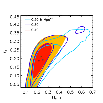
Figure 8: Stability of the estimates of $\Omega_{M}h$ and $f_{B}$ when varying the minimum fitting scale $k_{\rm{max}}$. The contours show 68 and 95% confidence levels. The filled contour corresponds to $k_{\rm{max}}=0.40\smash{\,h\,{\rm Mpc}^{-1}}$. The best-fit from each likelihood analysis is marked with a cross. No systematic trend with $k_{\rm{max}}$ is evident, confirming the conclusions drawn using the mock samples in Sect. 5.2.

6.3 Stability of the estimates with scale

Our extensive tests with mock data have indicated that our modelling of non-linear effects is fully adequate, with systematic errors well below the statistical uncertainties, which justified extending our likelihood analysis down to $k_{\rm max}=0.40\smash{\,h\,{\rm Mpc}^{-1}}$. But it is of interest to see whether the results from the real data display the same robustness to variations in $k_{\rm max}$ that we saw in the mocks.

We have thus repeated our analysis for $k_{\rm max}=0.20$, $0.30$ and $0.40\smash{\,h\,{\rm Mpc}^{-1}}$. The results in the plane $(\Omega_{M}h,f_{B})$ are compared in Fig. 8. This shows that, as seen with the mock samples, the best-fit values do not change significantly. Naturally, uncertainties are the largest for the lowest $k_{\rm max}$, since less information (fewer modes) is used.

6.4 Consistency with VIPERS PDR-1 estimates in configuration space

Using 60% of the full VIPERS data (the PDR-1 sample: Garilli et al. 2014), in Bel et al. (2014) we used the clustering ratio statistic in configuration space (see Bel & Marinoni 2014, for a definition), to derive the estimate of the matter density $\Omega_{M}=0.270^{+0.029}_{-0.025}$. To carry out a comparison we have repeated our likelihood estimates here with the same priors. We assume a flat $\Lambda$CDM cosmological model, described by parameter vector ${\bf p}=\{\Omega_{M},\Omega_{B}h^{2},H_{0},A_{s},n_{s},\sigma_{\rm TOT},b\}$. A flat prior for the matter density is assumed ($0.1$–$0.9$), while the other parameters are characterised by Gaussian priors $\Omega_{B}h^{2}=0.0213\pm 0.0010$ (from BBN: Pettini et al. 2008), $H_{0}=73.8\pm 0.024\,{\rm km\,s^{-1}Mpc^{-1}}$ (from HST: Riess et al. 2011), $\ln(10^{10}A_{s})=3.103\pm 0.072$ and $n_{s}=0.9616\pm 0.0094$ (Planck Collaboration et al. 2013). Bias and effective velocity dispersion $\sigma_{\rm TOT}$ are treated as in Sect. 6.2.

With these prior assumptions the power spectrum data yield a measurement of the matter density parameter ${\Omega_{M}=0.261^{+0.027}_{-0.027}}$. This value is in excellent agreement with the result of Bel et al. (2014) but it is in tension with the 2015 Planck result (Planck Collaboration et al. 2015). This apparent discrepancy derives from our adopted prior on $H_{0}$, which differs significantly from the Planck best-fit. As discussed in Bel & Marinoni (2014) it may be reconciled by the fact that the shape of the power spectrum is sensitive to the combination $\Omega_{M}h$ in the linear regime (which becomes $\Omega_{M}h^{2}$ on non-linear scales). As we will see in Sect. 7.1 the VIPERS constraints on $\Omega_{M}h$ are in much better consistency with the Planck measurements.

7 Discussion and Conclusions

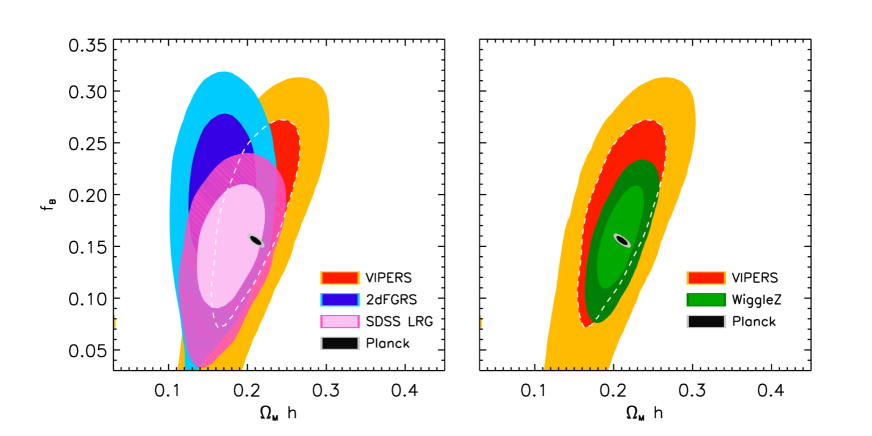
Figure 9: Comparison of VIPERS constraints on $f_{B}$ and $\Omega_{M}h$ with other galaxy surveys at low and high redshift. To test consistency with the cosmological model we have fixed the remaining cosmological parameters in the analysis of each survey. The expansion history is fixed to the fiducial model which restricts the allowed parameter space particularly at high redshift (compare with the VIPERS constraints in Fig. 7). Left panel: at low redshift we show the constraints from 2dFGRS at redshift $z=0.2$ (Cole et al. 2005a) and SDSS LRG at redshift $z=0.35$ (Tegmark et al. 2004b). Right panel: the constraints from WiggleZ (Parkinson et al. 2012) are shown. In both panels the constraints from Planck are overplotted (Planck Collaboration et al. 2015).

7.1 Comparison with previous redshift surveys

Comparing the VIPERS measurement with the constraints from datasets at different redshifts provides a consistency test of the cosmological model. To perform this test, we analyse other public datasets using the same set of priors as adopted for our own analysis (Sect. 6.2).

Our prime concern here is to see if the physical shape of the VIPERS $P(k)$ is consistent with constraints from other galaxy redshift surveys and from the Planck results. We therefore do not include Alcock-Paczyński effects and choose to fix the expansion history to the fiducial model with $\Omega_{M}=0.30$. This configuration allows us to test the consistency of $P(k)$ shape with maximum statistical power. We use the likelihood routines publicly available in the CosmoMC code (Lewis & Bridle 2002) to compute the constraints for 2dFGRS (Cole et al. 2005a), SDSS DR4 LRG (Tegmark et al. 2004b) and WiggleZ (Parkinson et al. 2012) as well as for the Planck 2015 measurements (Planck Collaboration et al. 2015).

The left panel of Fig. 9 shows the constraints on the $(\Omega_{M}h,f_{B})$ plane from the pioneering 2dFGRS measurements at redshift $z=0.2$ (Percival et al. 2001; Cole et al. 2005a). The 2dFGRS analysis used power data up to $k_{\rm max}=0.15\smash{\,h\,{\rm Mpc}^{-1}}$. We overplot the constraints from the SDSS LRG sample at redshift $z=0.35$. The SDSS LRG analysis used power data up to to $k_{\rm max}=0.20\smash{\,h\,{\rm Mpc}^{-1}}$. Both analyses marginalise over the parameters of the $Q$-model to fit the scale dependence of the power spectrum on small scales (Cole et al. 2005b). We find a lower value of $\Omega_{M}$ from 2dFGRS, although it is consistent with SDSS and Planck within the 95% confidence interval. The size of the likelihood region allowed by 2dFGRS and VIPERS is comparable, reflecting their similar survey volumes.

The right panel of Fig. 9 provides a similar comparison at higher redshift, contrasting the results of the present paper with the WiggleZ dataset (Parkinson et al. 2012; Blake et al. 2010). The WiggleZ analysis used power data up to $k_{\rm max}=0.20\smash{\,h\,{\rm Mpc}^{-1}}$ in each redshift bin ranging from $z=0.2$ to $z=0.8$. This is more conservative than $k_{\rm max}=0.30$ adopted in Parkinson et al. (2012). We find excellent agreement between the VIPERS and WiggleZ constraints and both are consistent with the Planck measurements.

7.2 Combined constraints

Given the consistency of the results found in Sect. 7.1, we may combine the constraints on the matter density and baryon fraction from the external LSS surveys. These constraints are most relevant if we allow the expansion history to vary according to the model; thus we now adopt the methodology described in Sect. 4.2 to account for the distance scaling. Again, we use the priors described in Sect. 6.2.

We compute the combined constraints from the external LSS surveys consisting of 2dFGRS, SDSS LRG and WiggleZ as shown in Fig. 10. We find this constraint to be fully consistent with VIPERS. Combining with the VIPERS likelihood gives the best available constraints from the LSS surveys to redshift $z=1.1$. We find marginalised values: $\Omega_{M}h=0.206_{-0.015}^{+0.013}$ and $f_{B}=0.170_{-0.025}^{+0.028}$. These values are consistent with the Planck ones, $\Omega_{M}h=0.211\pm 0.004$ and $f_{B}=0.158\pm 0.002$ (Planck Collaboration et al. 2015) within the statistical uncertainties.

It is interesting to ask if our determination of $\Omega_{M}h$ can shed any light on the disagreement concerning $H_{0}$ between Planck and direct measurements. For flat cosmological models, the angular location of the acoustic scale in the CMB temperature power spectrum is approximately sensitive to the parameter combination $\Omega_{M}h^{3}$, and this quantity should be robust even in the face of small scale-dependent systematics in Planck, which have been proposed as a possible explanation for the $H_{0}$ tension (Addison et al. 2016). Using the Planck temperature likelihood routine in CosmoMC we determine the marginalised value $\Omega_{M}h^{3}=0.0965\pm 0.0005$. Here we assume that the peak location is the dominant source for this constraint. Adopting the local estimate $H_{0}=73.24\pm 1.74\ \rm{km\,s^{-1}\,Mpc^{-1}}$ (Riess et al. 2016) leads to a low value of $\Omega_{M}h=0.180\pm 0.009$ indicated by the vertical shaded band in Fig. 10. This value is displaced from the full Planck constraint due to the 3.5$\sigma$ tension in the best-fit value of $H_{0}$. The combined LSS constraints lie between Planck and this lower value, and are consistent with both. The precision of current data therefore does not permit LSS to adjudicate in the $H_{0}$ dispute – but this diagnostic will sharpen with data from future surveys of larger volumes, and this is one way in which the $H_{0}$ debate could be resolved.

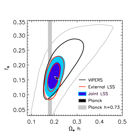
Figure 10: Joint parameter constraints from LSS surveys including 2dFGRS, SDSS LRG, WiggleZ, and VIPERS. The combined constraint including VIPERS is indicated by the solid contour. The reference from Planck is indicated by the ellipse. Rescaling the constraint on $\Omega_{M}h^{3}$ from the Planck temperature power spectrum using the local estimate of $H_{0}$ gives a prior on $\Omega_{M}h$ indicated by the vertical grey band.

7.3 Summary and Conclusions

In this paper we have presented the first measurement of the galaxy power spectrum from a sample extending beyond redshift $z=1$, using the final data from the VIMOS Public Extragalactic Redshift Survey (VIPERS). In particular

• we have discussed and tested in detail how the geometry and selection function of the VIPERS survey can be modelled, yielding an accurate description of the corresponding window function in Fourier space;

• we have tested and validated the corrections for all observation-specific effects affecting the VIPERS data, using a large set of custom-built mock samples. We similarly assessed the degree of modelling uncertainties related to non-linear clustering, galaxy biasing and redshift-space distortions. We show that residual systematic errors on the cosmological parameters deriving from these effects are about 20 times smaller than the statistical errors;

• we have presented new measurements of the power spectrum of galaxy clustering using 51,728 galaxies distributed within four independent subsamples defined by two redshift ranges $0.6<z<0.9$ and $0.9<z<1.2$ over the two VIPERS fields W1 and W4;

• we have used the set of mocks to estimate covariance matrices for all the measurements, and to access the range of scales where the effects of non-linear evolution on the shape of the power spectrum can be considered to be under control;

• we have used these ingredients to fit the data with a cosmological model for $P(k)$ with three free cosmological parameters ($\Omega_{M},f_{B},h$) and three parameters that encode galaxy physics (bias in each redshift bin and velocity dispersion); combining the four power spectrum measurements, this yields an estimate of the mean value of the matter density (scaled to the current epoch), $\Omega_{M}h=0.227^{+0.063}_{-0.050}$, and baryon fraction $f_{B}=0.220^{+0.058}_{-0.072}$, after marginalising over galaxy bias;

• these values, which describe the galaxy distribution when the Universe was about half its current age, are in agreement with measurements at lower redshift from 2dFGRS at $z=0.2$, SDSS LRG at $z=0.35$, and WiggleZ at $0.2<z<0.8$. We further demonstrate consistency with the Planck determination of $\Omega_{M}h$ and $f_{B}$;

• comparison to previous configuration space constraints on $\Omega_{M}$ from VIPERS (counts in cells) shows consistency despite the intrinsically different nature of the measurements and their covariances.

These results have extended the classical cosmological test of determining the matter content of the Universe from the shape of the galaxy power spectrum. There is no reason to believe that this method has reached the limit of its precision, and we expect the error contours to continue to shrink with new generations of larger galaxy surveys. In this way, the galaxy power spectrum has the potential to clarify current areas of cosmological uncertainty, such as the true value of $H_{0}$.