The VIMOS Public Extragalactic Redshift Survey (VIPERS): Galaxy segregation inside filaments at $z\simeq 0.7$

Abstract

We present the first quantitative detection of large-scale filamentary structure at $z\simeq 0.7$ in the large cosmological volume probed by the VIMOS Public Extragalactic Redshift Survey (VIPERS). We use simulations to show the capability of VIPERS to recover robust topological features in the galaxy distribution, in particular the filamentary network. We then investigate how galaxies with different stellar masses and stellar activities are distributed around the filaments and find a significant segregation, with the most massive or quiescent galaxies being closer to the filament axis than less massive or active galaxies. The signal persists even after down-weighting the contribution of peak regions. Our results suggest that massive and quiescent galaxies assemble their stellar mass through successive mergers during their migration along filaments towards the nodes of the cosmic web. On the other hand, low-mass star-forming galaxies prefer the outer edge of filaments, a vorticity rich region dominated by smooth accretion, as predicted by the recent spin alignment theory. This emphasizes the role of large scale cosmic flows in shaping galaxy properties.

1 Introduction

A major success of the $\Lambda$CDM model is its ability to reproduce the wealth of large-scale structures (LSS) observed in the galaxy distribution (e.g. Springel et al., 2006). These structures arise from the growth of primordial, nearly Gaussian, matter density fluctuations under the effect of gravity. In this process, matter departs from underdense regions and flows through dense sheets that wind up, forming filaments along which matter drifts and progressively gets accreted onto high-density peaks. This leads to a cosmic web (CW) where dense nodes are connected by filaments, framing walls separated by large voids (Bond et al., 1996). The baryonic gas follows the gravitational potential gradients imposed by the dark matter distribution, then is shocked, forming (among other structures) tenuous ionised hydrogen filaments, the intergalactic medium (IGM), in which galaxies can form. These filaments are regions where gas, momentum, and energy are exchanged through the complex processes of infall and outflow. While it has long been established that the local density environment on typical scales below a few Mpc plays a role in shaping galaxy properties (see e.g. Dressler, 1980; Zehavi et al., 2005), the extent to which large-scale anisotropic structures and the tidal field of the CW influence the evolution of galaxies (and subsequently properties such as morphology, accretion mode, and merging rate) still remains an open issue.

There is significant numerical evidence that large-scale environment has an impact on the formation and evolution of galaxies. In particular, N-body dark matter simulations have shown that the spin and the shape of dark matter haloes depend on the large-scale environment in which they reside (Aragón-Calvo et al., 2007; Hahn et al., 2007; Sousbie et al., 2009). Moreover, using hydrodynamical simulations, Kereš et al. (2005) found that at high redshift cold streams can penetrate deep inside haloes and feed galaxies with fresh gas to sustain intense star formation (SF) activity (see also Dekel et al., 2009; Dekel & Birnboim, 2006). Pichon et al. (2011) proposed that the filamentary flows advect angular momentum onto the disks of galaxies and that the spin of newly formed galaxies tends preferentially to be parallel to the axis of their closest filament. Codis et al. (2012) quantified a mass transition, with the most massive haloes ending up with a spin perpendicular to the filaments as a result of successive mergers along the filaments. These results have been extended to galaxies by Dubois et al. (2014) with the state-of-the-art hydrodynamical simulation Horizon-AGN (see also Codis et al., 2015, for a theoretical motivation for this transition based on constrained tidal torque theory). On the side of observations, the correlation between the spin of galaxies and their filaments or sheets has been recently detected in the Sloan Digital Sky Survey (Tempel et al., 2013; Zhang et al., 2013; Trujillo et al., 2006). This remarkable result confirms the role played by the large scale dynamical environment in the evolution of galaxies, which is usually neglected in galaxy formation models (e.g. Zehavi et al., 2005; Guo et al., 2011).

In the local Universe ($z\leq 0.3$) the large galaxy redshift surveys 2dF (Colless et al., 2001), SDSS (York et al., 2000), and GAMA (Driver et al., 2011) have captured the CW in great detail and led to several analyses showing variations of individual (Beygu et al., 2013; Alpaslan et al., 2015, 2016) and statistical (Eardley et al., 2015; Martínez et al., 2016) galaxy properties as a function of their CW environment. At higher redshifts, because of the small volumes probed and the low sampling rates achieved by redshift surveys, this kind of analysis has not been possible until recently. The state-of-the-art redshift survey VIPERS (Guzzo et al., 2014) overcomes these limitations by probing a volume equivalent to the local 2dF survey with a dense spectroscopic sampling of galaxies. It allowed the first measurement of the growth rate of the LSS at $0.5\leq z\leq 1.2$ (de la Torre et al., 2013) and the fine mapping of the CW at an epoch when the Universe was about half its current age.

In this paper, we exploit the final, complete sample of the VIPERS survey to detect the filamentary structure of the CW at high redshift and to study the correlation between galaxy properties and their distance to the closest filament. After describing the data in Sect. 2, we illustrate in Sect. 3 the filament reconstruction with the Discrete Persistent Structure Extractor (DisPerSE, Sousbie, 2011) on mock samples of the VIPERS survey and its fidelity. We present the application to the VIPERS data in Sect. 4, where we also report a significative mass and type segregation within filaments. Finally, we discuss in Sect. 5 our results within the current paradigm of galaxy assembly. Unless stated otherwise, we assume the Planck Collaboration et al. (2015) cosmology with $H_{0}=67.51$ km s^-1 Mpc^-1, $h=H_{0}/100$, $\Omega_{m}=0.3121$, and $\Omega_{\Lambda}=0.6879$.

2 Data

The VIMOS Public Extragalactic Redshift Survey (VIPERS) is a magnitude-limited spectroscopic galaxy survey to $i_{AB}\leq 22.5$. It covers an overall footprint of about $16\deg^{2}$ and $8\deg^{2}$ in the W1 and W4 fields of the CFHTLS-Wide imaging survey, respectively. VIPERS spectra were collected in low resolution mode, $R=230$, leading to a radial velocity error of $\sigma_{v}=175(1+z_{\rm spec})$ km s^-1. The spectroscopic targets were pre-selected in a colour-colour space to remove galaxies below $z=0.5$, which coupled with an optimized observing strategy, provides an average effective sampling rate of about $40\%$. We refer the reader to the survey description papers by Guzzo et al. (2014) and Garilli et al. (2014) and to the parallel paper by Scodeggio et al. (2016) for more details.

In this work we use the final galaxy sample, described in the latter paper (the so-called PDR-2). We consider only the most secure redshifts, corresponding to quality flag $\geq 2$ in the VIPERS grading scheme (confidence level, CL $>97\%$). The mean number density of galaxies, $\overline{n}(z)$, varies significantly at the redshift boundaries of the survey, due to the magnitude limit, the target sampling rate, and the colour selection (see de la Torre et al., 2013; Guzzo et al., 2014, for details). For this reason we limit this analysis to the 50 980 galaxies in the range $0.5\leq z\leq 0.85$, where the typical spatial resolution in terms of mean inter-galaxy separation, $\langle D_{z}\rangle\sim\overline{n}{(z)}^{-1/3}$, is the highest ($7.7<\langle D_{z}\rangle/\mathrm{Mpc}<10$). These values are comparable with those of the GAMA survey (Driver et al., 2011, with $4.6<\langle D_{z}\rangle/\mathrm{Mpc}<8.8$ for $0.1<z<0.3$ and $r\leq 19.8$), and make VIPERS the first galaxy redshift survey well suited for studying the CW at high redshift. The stellar masses for the objects in our sample and the classification between active and passive populations were derived according to Moutard et al. (2016b), on the basis of the SED-fitting analysis of the multi-wavelength data collected in the VIPERS regions (Moutard et al., 2016a).

3 Detecting filaments in the VIPERS survey

The DisPerSE code.

In order to trace the CW in VIPERS, we rely on the Discrete Persistent Structure Extractor (DisPerSE, see Sousbie, 2011; Sousbie et al., 2011, for a complete description). DisPerSE identifies filaments as ridges in the density field (calculated using the Delaunay Tessellation Field Estimator, DTFE). DisPerSE uses the discrete Morse theory to extract critical points, where the gradient of the density field vanishes (e.g. maxima and saddle points), and the field lines connecting them. It then pairs the critical points in topological features, called “critical pairs”, using the persistent homology theory. The robustness of each feature (including the filaments) is assessed by the relative density contrast of its critical pair, the so-called persistence, which is chosen to pass a certain signal-to-noise (S/N) threshold. The noise level is defined relative to the variance of persistence values obtained from random sets of points. Because DisPerSE is based on a topologically-motivated algorithm, it is both very robust and flexible through the choice of the persistence threshold. Since it filters out the sampling noise, it enables an unsmoothed density field, more noisy but less biased, to be analysed. By construction it is also multi-scale: it builds a network which adapts naturally to the uneven sampling of observed catalogues. The persistence threshold is calibrated on mocks to account for the specific design of VIPERS. To prevent the spurious detection of filaments near the edges of the survey, DisPerSE encloses each field in a larger volume. New particles are added by interpolating the density field measured at the boundary of the survey (see e.g. Sousbie et al., 2011).

Tests on VIPERS mock galaxy catalogues.

We test the performance of DisPerSE on an updated version of the VIPERS mock galaxy catalogues described in de la Torre et al. (2013) matching the VIPERS final geometry. The upgrades are described in the parallel paper by de la Torre et al. (2016). The parent catalogues include all the galaxies down to the magnitude limit $i_{AB}=22.5$ together with the correct selection function at $0.4<z<0.6$ due to the VIPERS colour pre-selection. The VIPERS-like catalogues are built from the parent ones with all the observational effects applied (i.e. pointing strategy, target sampling rate, gaps between VIMOS quadrants, photometric mask and random errors on redshift).

The impact of observational biases on the skeleton reconstruction can be assessed by comparing the skeletons obtained from the parent and the VIPERS-like mock catalogues. To quantify the differences between two skeletons we define a pseudo-distance between the two skeletons to be compared. In practice, a skeleton S_a is composed by $N_{a}$ short straight segments, s${}_{a}^{i}$. We define the pseudo-distance from a skeleton S_a to a skeleton S_b, D(S_a, S_b), as the probability distribution function (PDF) of the distances between each segment of S_a, s${}_{a}^{i}$, and its closest segment in S_b, s${}_{b}^{j}$ (Sousbie et al., 2009). The distributions D(S_a, S_b) and D(S_b, S_a) are composed by $N_{a}$ and $N_{b}$ distances respectively. There is no reason for the pseudo-distance D(S_a, S_b) to be identical to D(S_b, S_a). Indeed the discrepancy between the two PDFs is related to the differences between the two skeletons.

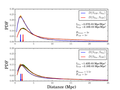
Figure 1: PDFs of the pseudo-distances (defined in Sect. 3) between the Parent and VIPERS-like skeletons. Blue lines and orange shaded areas refer to S_VIP projected onto S_Par while red lines and green shaded areas are the reverse. Solid lines correspond to the mean of 10 mocks and the shaded areas enclose the $1\sigma$ r.m.s. (please note that uncertainties are negligible). Arrows show the modes of the distributions. Top: The two skeletons are extracted with a $3\sigma$ persistence threshold. Bottom: S_Par is extracted with a $5.5\sigma$ threshold.

Fig. 1 presents the PDFs of the pseudo-distances obtained by comparing the skeletons S_Par and S_VIP measured from the Parent and VIPERS-like catalogues, respectively, in the redshift range $0.5<z<0.85$. In the upper panel, DisPerSE is run with a persistence threshold of $3\sigma$ in both catalogues. This threshold guarantees that less than 1% of critical pairs are spurious, as tested on random field simulations (Sousbie, 2011). S_VIP is reconstructed with less accuracy and detail due to the lower sampling. An estimate of the uncertainty in the location of the filaments is given by the modes of the PDFs which do not peak at distance $D\sim 0$ (corresponding to a perfect match between the segments of the two skeletons) but $D\sim 1.5-2$ Mpc (marked as vertical arrows). The asymmetry between D($S_{\rm Par},S_{\rm VIP}$) and D($S_{\rm VIP},S_{\rm Par}$) reflects the fact that S_Par (full sampling) has much more details (i.e. the leaves of branches, or small branches) which have no counterpart in $S_{\rm VIP}$. On the other hand 90% of the segments of $S_{\rm VIP}$ have a counterpart in $S_{\rm Par}$ with distances $D\leq 10$ Mpc, illustrating the small fraction of spurious filaments. We also report the average length of the VIPERS-like (L_VIP) and the Parent (L_Par) skeletons, defined as the total skeleton length divided by the survey volume (expressed in Mpc/Mpc³). L_VIP is shorter than L_Par as expected for a skeleton with fewer details. In the lower panel, the persistence threshold on the Parent catalogue is increased to 5.5$\sigma$. The length, L_Par, is shortened with only the most significant filaments still present. The two PDFs for D($S_{\rm VIP},S_{\rm Par}$) and D($S_{\rm Par},S_{\rm VIP}$) are now much closer in amplitude and shape. Most of the segments in $S_{\rm Par}$ (75%) have a counterpart in $S_{\rm VIP}$ with $D\leq 10$ Mpc. The modes of the distributions are almost unchanged. Even if the two skeletons are more similar, the skeleton $S_{\rm VIP}$ tends to oscillate around its true location (as reconstructed by $S_{\rm Par}$), making the length L_VIP longer than L_Par.

In conclusion, the close match between the two PDFs indicates that the skeleton reconstructed at 3$\sigma$ for the VIPERS-like catalogue is able to detect the most robust filaments (corresponding to a $5.5\sigma$ persistence threshold in a fully sampled dataset) and contains a small fraction of spurious filaments.

4 Results

The filamentary structures of the Cosmic Web.

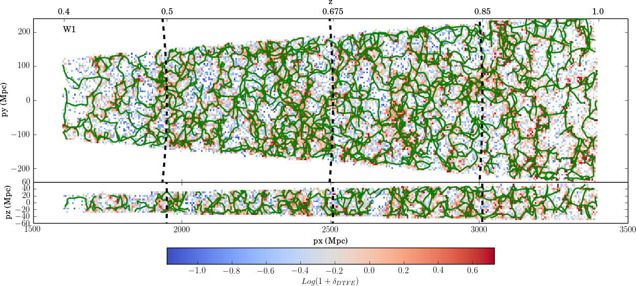
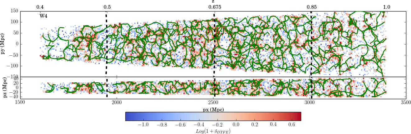
Figure 2: Projected distribution of the filaments reconstructed with DisPerSE (in dark green) in the VIPERS W1 (top panel) and W4 (bottom panel) fields between $0.4\leq z\leq 1$. The density contrast, $\log(1+\delta_{\rm DTFE})$, is averaged on cells of $5\times 5$ Mpc² and colour-coded as indicated (white for empty cells). Top rows: projected distribution along the declination direction ($\Delta\delta=2$). Bottom rows: projected distribution along the right ascension direction (in the central regions with $\Delta\alpha=2$). 3D movies are available on the VIPERS website.

We run DisPerSE on the VIPERS fields with a $3\sigma$ persistence threshold. Fig. 2 shows the filamentary network (green lines) for W1 (top panels) and W4 (bottom panels) fields, overplotted on a map of the density contrast $\delta={n_{\rm DTFE}}/{\overline{n}(z)}-1$, where $n_{\rm DTFE}$ is the local DTFE density estimate. Even in the 2D projections, we can see that filaments reveal the ridges of the 3D density field which, by construction, connect the density peaks between them via saddle points. The averaged length of the skeletons are similar with $L\sim$ 0.0013 and 0.0016 Mpc/Mpc³ in W1 and W4 respectively. At low ($z\leq 0.5$) and high redshift ($z\geq 0.85$), the number of filaments drops as a consequence of the lower sampling and only the most secure filaments are detected, as expected with DisPerSE. Thanks to the large contiguous volume probed by VIPERS, large voids, partly delineated by the filaments, are visible in both fields with radii as large as $R\sim 30$ Mpc (see Micheletti et al. 2014 and the parallel paper by Hawken et al. 2016 for void analysis in VIPERS).

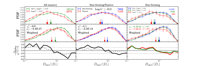
Figure 3: Distributions of the unweighted (top row) and density-weighted (middle row) normalised distances ($D_{\rm skel}/\langle D_{z}\rangle$), for three selections: low vs high mass galaxies (left column), quiescent vs star-forming galaxies (middle column) and star-forming galaxies in three mass bins (right column). Vertical arrows indicate the medians of the PDFs and errorbars represent the dispersions computed with block-wise jackknife resampling. The PDFs after reshuffling of the samples (see text) are shown with dashed lines. The differences between the weighted distributions are shown in the bottom row. For star-forming galaxies (right panel) only the differences between high-intermediate (green) and high-low (red) mass bins are shown. The values resulting from the $\chi^{2}$ test of independence are reported in the middle panels.

Mass segregation inside filaments.

We now investigate how different galaxy populations are distributed within this filamentary network in the redshift range $0.5\leq z\leq 0.85$. We measure the distance of each galaxy to the nearest filament, $D_{\rm skel}$ (which, in the figure, we report normalised to $\langle D_{z}\rangle$ to take care of the variations of the mean inter-galaxy separation across the redshift range considered). The normalised PDFs of the distances, in the W1 and W4 fields combined, are shown in Fig. 3 for three selections: low vs high mass galaxies, star-forming vs quiescent galaxies, and star-forming galaxies in three mass bins. The errorbars are estimated with a block-wise ($1\deg^{2}$) jackknife resampling. The first two samples are limited to $M^{\ast}\geq 10^{10.5}M_{\sun}$ to be complete in stellar mass for both quiescent and star-forming galaxies (see Davidzon et al., 2016) while a mass cut of $M^{\ast}\sim 10^{10}M_{\sun}$ is used when only star-forming galaxies are considered.

A trend between distance and stellar mass is observed (left column), with more massive galaxies being closer to filaments as indicated by the shift in the median values of the two PDFs (downward arrows). Passive galaxies are also found to be closer to filaments (middle column). While a large fraction ($47\%$) of our massive ($M^{\ast}\geq 10^{10.5}M_{\sun}$) galaxies are also passive, by looking at the star-forming population alone we observe a similar trend, albeit weaker, with the most massive star-forming galaxies being closer to filaments (right column). However, since we wish to evaluate the impact of the filaments on galaxy properties, we have to take into account the contribution of the nodes of the density field, usually related to galaxy groups and clusters, which are at the intersections of filaments and are known to be privileged regions where quenching is more efficient. This task is not easy, as there are partial overlaps between the local density and the CW environment (Aragón-Calvo et al., 2010). As proposed by Gay et al. (2010), to minimize the node contributions we weight each galaxy by the inverse of the density field smoothed using a Gaussian filter with $\sigma=3$ Mpc. The weighted PDFs are shown in the middle row of Fig. 3. A shift in the medians of the PDFs to larger distances is observed but the trends remain. We also adopted alternative approaches by rejecting galaxies in high density regions ($\delta\geq 4$), located within groups, according to a parallel analysis (Iovino et al., in prep.), or by keeping only the filaments with a higher persistence threshold. They do not qualitatively change the results discussed in this section.

The significance of the observed trends is illustrated by the residuals between the weighted distributions expressed in units of $\sigma$ (bottom row of Fig. 3). The deviations exceed $2\sigma$ in most of the bins except for star-forming samples alone (due to shot noise in the most massive bin). We also quantify the differences with the $\chi^{2}$ test of independence and the probabilities of observing such a difference by chance which are negligible (listed in middle panels). This confirms the existence of a weak but statistically significant segregation effect inside the filaments and suggests that galaxy processing happens also during the drift of galaxies towards the nodes of the CW.

In Fig. 3 we also look at how the mass-density relation is hidden in the observed mass segregation. We split the sample in local density bins and reshuffle the stellar masses between the galaxies in each bin. The mean PDF distributions for 10 random reshufflings are shown as dashed lines on the middle left panel. The PDFs for the low and high mass bins are close to the original ones, which shows that the mass segregation exists even after reshuffling the masses, if the mass-density relation is preserved. Therefore the mass segregation inside the filaments emerges naturally from the mass-density relation and the anisotropic distribution of the density in the CW.

A similar approach is adopted for the galaxy type segregation. We randomly attribute a galaxy type (passive/star-forming) to galaxies by conserving the type fraction observed in different stellar mass bins. The mean PDFs for 10 random reshufflings are shown as dashed lines (middle panel). In this case the segregation almost vanishes, with a difference between the two PDFs of less than $1\sigma$. The observed type segregation therefore does not arise just from the mass-type fraction relation but could have its origin in the dynamic of the large scale anisotropic structures of the CW.

5 Discussion and conclusions

We reported the first characterization of large scale filamentary structures at $z\sim 0.7$, carried out in the cosmological volume probed by the VIPERS spectroscopic survey. The reconstruction is based on the DisPerSE code and the capability of VIPERS to capture such a CW’s filamentary network is tested on simulations. We observe a small but significant trend for galaxies with different stellar masses and stellar activity to segregate near the filaments with the most massive and/or passive galaxies being closer to filaments. The signal persists even after down-weighting the contribution of nodes and high density regions.

The galaxy segregation quantified in this paper is a first step in support of a new paradigm in galaxy formation where large scale cosmic flows play a role in shaping galaxy properties. Beyond the observed anisotropy of the mass distribution (which follows naturally from the mass-density relation and the anisotropy of density in the CW), we expect that other physical parameters (e.g. stellar activity controlled in part by gas accretion or morphology and size controlled in part by angular momentum) will be impacted by this large scale environment. Indeed, our results are fully consistent with the ingredients of the spin alignment theory presented in Codis et al. (2015) which relies on these large-scale cosmic flows. The stellar activity segregation observed here can be interpreted inside this theory. Low mass or star-forming galaxies are preferentially located at the outskirts of filaments, a vorticity rich environment (Laigle et al., 2015), where galaxies acquire both their angular momentum (leading to a spin parallel to the filaments) and their stellar mass essentially via smooth accretion (Welker et al., 2015). The stellar-mass segregation observed here is the next step, where at higher mass, a transition is predicted in simulations, when more massive post-mergers drifting along filaments convert the orbital momentum of their progenitors into spin perpendicular to the axis of the filament, with increased efficiency for higher merger rate (Dubois et al., 2014; Welker et al., 2015). The most massive galaxies, dominated by the quiescent population, should preferentially complete their stellar mass assembly in the core of filaments by merging.

We plan to extend the characterization of the CW in VIPERS in a future paper. It will be of interest to extend our analysis to other physical quantities such as star-formation rate or specific star-formation rate, spin orientation and extent to different CW perspective: the distance to nodes within the filaments or, of particular interest, the distance from the saddle of the filaments, expected to be the region in the filament where galaxies have been the less affected by environmental effects. This will become within reach with the upcoming large and deep spectroscopic surveys such as PFS (Prime Focus Spectrograph). With its higher sampling and high-redshift extension ($z\sim 1.5-2$), PFS-deep survey will offer the opportunity to explore such dependencies near the peak of the cosmic star formation activity with an unprecedented accuracy.

Meanwhile, alternative approaches based on large multi-band photometric surveys (e.g. COSMOS, J-PAS, Benitez et al. 2014) with accurate photometric redshifts allow us to analyze the projected 2D CW in narrow redshift slices. Preliminary results on the filamentary structures in the COSMOS field yield consistent results for the mass segregation inside the filaments (Laigle et al., in prep.).

References

- Alpaslan et al. (2015) Alpaslan M., et al., 2015, MNRAS, 451, 3249
- Alpaslan et al. (2016) Alpaslan M., et al., 2016, MNRAS, 457, 2287
- Aragón-Calvo et al. (2007) Aragón-Calvo M. A., van de Weygaert R., Jones B. J. T., van der Hulst J. M., 2007, ApJ, 655, L5
- Aragón-Calvo et al. (2010) Aragón-Calvo M. A., Platen E., van de Weygaert R., Szalay A. S., 2010, ApJ, 723, 364
- Aragon-Calvo et al. (2015) Aragon-Calvo M. A., Weygaert R. v. d., Jones B. J. T., Mobasher B., 2015, MNRAS, 454, 463
- Benitez et al. (2014) Benitez N., et al., 2014, preprint, (arXiv:1403.5237)
- Beygu et al. (2013) Beygu B., Kreckel K., van de Weygaert R., van der Hulst J. M., van Gorkom J. H., 2013, AJ, 145, 120
- Bond et al. (1996) Bond J. R., Kofman L., Pogosyan D., 1996, Nature, 380, 603
- Chisari et al. (2015) Chisari N., et al., 2015, MNRAS, 454, 2736
- Codis et al. (2012) Codis S., Pichon C., Devriendt J., Slyz A., Pogosyan D., Dubois Y., Sousbie T., 2012, MNRAS, 427, 3320
- Codis et al. (2015) Codis S., Pichon C., Pogosyan D., 2015, MNRAS, 452, 3369
- Colless et al. (2001) Colless M., et al., 2001, MNRAS, 328, 1039
- Davidzon et al. (2016) Davidzon I., et al., 2016, A&A, 586, A23
- Dekel & Birnboim (2006) Dekel A., Birnboim Y., 2006, MNRAS, 368, 2
- Dekel et al. (2009) Dekel A., et al., 2009, Nature, 457, 451
- Dressler (1980) Dressler A., 1980, ApJ, 236, 351
- Driver et al. (2011) Driver S. P., et al., 2011, MNRAS, 413, 971
- Dubois et al. (2014) Dubois Y., et al., 2014, MNRAS, 444, 1453
- Eardley et al. (2015) Eardley E., et al., 2015, MNRAS, 448, 3665
- Garilli et al. (2014) Garilli B., et al., 2014, A&A, 562, A23
- Gay et al. (2010) Gay C., Pichon C., Le Borgne D., Teyssier R., Sousbie T., Devriendt J., 2010, MNRAS, 404, 1801
- Guo et al. (2011) Guo Q., et al., 2011, MNRAS, 413, 101
- Guzzo et al. (2014) Guzzo L., et al., 2014, A&A, 566, A108
- Hahn et al. (2007) Hahn O., Porciani C., Carollo C. M., Dekel A., 2007, MNRAS, 375, 489
- Hawken et al. (2016) Hawken A. J., et al., 2016, in prep.
- Kereš et al. (2005) Kereš D., Katz N., Weinberg D. H., Davé R., 2005, MNRAS, 363, 2
- Laigle et al. (2015) Laigle C., et al., 2015, MNRAS, 446, 2744
- Martínez et al. (2016) Martínez H. J., Muriel H., Coenda V., 2016, MNRAS, 455, 127
- Micheletti et al. (2014) Micheletti D., et al., 2014, A&A, 570, A106
- Moutard et al. (2016a) Moutard T., et al., 2016a, A&A, 590, A102
- Moutard et al. (2016b) Moutard T., et al., 2016b, A&A, 590, A103
- Pichon et al. (2011) Pichon C., Pogosyan D., Kimm T., Slyz A., Devriendt J., Dubois Y., 2011, MNRAS, 418, 2493
- Planck Collaboration et al. (2015) Planck Collaboration et al., 2015, preprint, (arXiv:1502.01589)
- Scodeggio et al. (2016) Scodeggio M., et al., 2016, in prep.
- Sousbie (2011) Sousbie T., 2011, MNRAS, 414, 350
- Sousbie et al. (2009) Sousbie T., Colombi S., Pichon C., 2009, MNRAS, 393, 457
- Sousbie et al. (2011) Sousbie T., Pichon C., Kawahara H., 2011, MNRAS, 414, 384
- Springel et al. (2006) Springel V., Frenk C. S., White S. D. M., 2006, Nature, 440, 1137
- Tempel et al. (2013) Tempel E., Stoica R. S., Saar E., 2013, MNRAS, 428, 1827
- Trujillo et al. (2006) Trujillo I., Carretero C., Patiri S. G., 2006, ApJ, 640, L111
- Welker et al. (2015) Welker C., Dubois Y., Devriendt J., Pichon C., Kaviraj S., Peirani S., 2015, preprint, (arXiv:1502.05053)
- York et al. (2000) York D. G., et al., 2000, AJ, 120, 1579
- Zehavi et al. (2005) Zehavi I., et al., 2005, ApJ, 630, 1
- Zhang et al. (2013) Zhang Y., Yang X., Wang H., Wang L., Mo H. J., van den Bosch F. C., 2013, ApJ, 779, 160
- de la Torre et al. (2013) de la Torre S., et al., 2013, A&A, 557, A54
- de la Torre et al. (2016) de la Torre S., et al., 2016, in prep.