Scalable Approximations for Generalized Linear Problems

Abstract

In stochastic optimization, the population risk is generally approximated by the empirical risk. However, in the large-scale setting, minimization of the empirical risk may be computationally restrictive. In this paper, we design an efficient algorithm to approximate the population risk minimizer in generalized linear problems such as binary classification with surrogate losses and generalized linear regression models. We focus on large-scale problems, where the iterative minimization of the empirical risk is computationally intractable, i.e., the number of observations $n$ is much larger than the dimension of the parameter $p$, i.e. $n\gg p\gg 1$. We show that under random sub-Gaussian design, the true minimizer of the population risk is approximately proportional to the corresponding ordinary least squares (OLS) estimator. Using this relation, we design an algorithm that achieves the same accuracy as the empirical risk minimizer through iterations that attain up to a cubic convergence rate, and that are cheaper than any batch optimization algorithm by at least a factor of $\mathcal{O}(p)$. We provide theoretical guarantees for our algorithm, and analyze the convergence behavior in terms of data dimensions. Finally, we demonstrate the performance of our algorithm on well-known classification and regression problems, through extensive numerical studies on large-scale datasets, and show that it achieves the highest performance compared to several other widely used and specialized optimization algorithms.

1 Introduction

We consider the following optimization problem

$$\underset{\beta\in{\mathbb{R}}^{p}}{\text{minimize}}\ R(\beta)\coloneqq\mathbb{E}\left[\vphantom{\big{[}}\Psi\left({\langle x,\beta\rangle}\right)-y{\langle x,\beta\rangle}\right],$$ (1.1)

where $\Psi:{\mathbb{R}}\to{\mathbb{R}}$ is a non-linear function, $y\in\mathcal{Y}\subset{\mathbb{R}}$ denotes the response variable, $x\in\mathcal{X}\subset{\mathbb{R}}^{p}$ denotes the predictor (or covariate), and the expectation is over the joint distribution of $(y,x)$. The above minimization is called a generalized linear problem in its canonical representation, and it is commonly encountered in the statistical learning. Celebrated examples include binary classification with smooth surrogate losses [BSS05, RW10], and generalized linear models (GLMs) such as Poisson regression, logistic regression, ordinary least squares, multinomial regression and many applications involving graphical models [NB72, MN89, WJ08, KF09]. These methods play a crucial role in numerous machine learning and statistics problems, and provide a miscellaneous framework for many regression and classification tasks.

The exact minimization of the stochastic optimization problem (1.1), requires the knowledge of the underlying distribution of the variables $(y,x)$. In practice, however, the joint distribution is not available. Therefore, after observing $n$ independent data points $(y_{i},x_{i})$, the standard approach is to minimize the empirical risk approximation given as

$$\underset{\beta\in{\mathbb{R}}^{p}}{\text{minimize}}\ \widehat{R}(\beta)\coloneqq\frac{1}{n}\sum_{i=1}^{n}\Psi\left({\langle x_{i},\beta\rangle}\right)-y_{i}{\langle x_{i},\beta\rangle}\,.$$ (1.2)

In the case of GLMs, the empirical risk minimization given in (1.2) is called the maximum likelihood estimation, whereas in the case of binary classification, it is generally referred to as surrogate loss minimization. Due to non-linear structure of the optimization task given in (1.2), for both problems, the minimization of the empirical risk requires iterative methods. Regardless of the problem formulation, the most commonly used optimization method is the Newton-Raphson method, which may be viewed as a reweighted least squares algorithm [MN89, BSS05]. This method uses a second-order approximation to benefit from the curvature of the log-likelihood and achieves locally quadratic convergence. A drawback of this approach is its excessive per-iteration cost of $\mathcal{O}(np^{2})$. To remedy this, Hessian-free Krylov sub-space based methods such as conjugate gradient and minimal residual are used, but the resulting direction is imprecise [HS52, PS75, Mar10]. On the other hand, first-order approximation yields the gradient descent algorithm, which attains a linear convergence rate with $\mathcal{O}(np)$ per-iteration cost. Although its convergence rate is slow compared to that of the second-order methods, its modest per-iteration cost makes it practical for large-scale problems. In the regime $n\gg p$, another popular optimization technique is the class of Quasi-Newton methods [Bis95, Nes04], which can attain a per-iteration cost of $\mathcal{O}(np)$, and the convergence rate is locally super-linear; a well-known member of this class of methods is the BFGS algorithm [Bro70, Fle70, Gol70, Sha70]. There are recent studies that exploit the special structure of GLMs [Erd15a], and achieve near-quadratic convergence with a per-iteration cost of $\mathcal{O}\left(np\right)$, and an additional cost of covariance estimation.

In this paper, we take an alternative approach for minimizing (1.1), based on an identity that is well-known in some areas of statistics, but appears to have received relatively little attention for its computational implications in large-scale problems. Let $\beta^{\sf pop}$ denote the true minimizer of the population risk given in (1.1), and let $\beta^{\sf ols}$ denote the corresponding ordinary least squares (OLS) coefficients defined as $\beta^{\sf ols}=\mathbb{E}\left[xx^{T}\right]^{-1}\mathbb{E}\left[xy\right]$. Then, under certain random predictor (design) models,

$$\beta^{\sf pop}\propto\beta^{\sf ols}.$$ (1.3)

For logistic regression with Gaussian design (which is equivalent to Fisher’s discriminant analysis), (1.3) was noted by Fisher in the 1930s [Fis36]; a more general formulation for models with Gaussian design is given in [Bri82]. The relationship (1.3) suggests that if the constant of proportionality is known, then $\beta^{\sf pop}$ can be estimated by computing the OLS estimator, which may be substantially simpler than minimizing the empirical risk. In fact, in some applications like binary classification, it may not be necessary to find the constant of proportionality in (1.3). Our work in this paper builds on this idea.

Our contributions can be summarized as follows.

1. We show that $\beta^{\sf pop}$ is approximately proportional to $\beta^{\sf ols}$ in the random design setting, regardless of the covariate (predictor) distribution. That is, we prove

   $$\left\|\beta^{\sf pop}-c_{\Psi}\times\beta^{\sf ols}\right\|_{\infty}\lesssim\frac{1}{p},$$

   for some $c_{\Psi}\in{\mathbb{R}}$ which depends on the non-linearity $\Psi$. Our generalization uses zero-bias transformations [GR97]. We also show that the above relation still holds under certain types of regularization.

2. We design a computationally efficient estimator for $\beta^{\sf pop}$ by first estimating the OLS coefficients, and then estimating the proportionality constant $c_{\Psi}$ via line search. We refer to the resulting estimator as the Scaled Least Squares (SLS) estimator and denote it by $\hat{\beta}^{\sf\hskip 0.72229ptsls}$. After estimating the OLS coefficients, the second step of our algorithm involves finding a root of a real valued function; this can be accomplished using iterative methods with up to a cubic convergence rate and only $\mathcal{O}(n)$ per-iteration cost. This is cheaper than the classical batch methods mentioned above by at least a factor of $\mathcal{O}(p)$.

3. For random design with sub-Gaussian predictors, we show that

   $$\left\|\hat{\beta}^{\sf\hskip 0.72229ptsls}-\beta^{\sf pop}\right\|_{\infty}\lesssim\frac{1}{p}+\sqrt{\frac{p}{n/\log(n)}}.$$

   This bound characterizes the performance of the proposed estimator in terms of data dimensions, and justifies the use of the algorithm in the regime $n\gg p\gg 1$.

4. We demonstrate how to transform a binary classification problem with smooth surrogate loss into a generalized linear problem, and how our methods can be applied to obtain a computationally efficient optimization scheme. We further discuss the canonicalization of the square loss, which may be of independent interest to non-convex optimization community.

5. We propose a scalable algorithm for converting one generalized linear problem to another by exploiting the proportionality relation (1.3). The proposed algorithm requires only $\mathcal{O}\left(n\right)$ per each iteration, with no additional cost.

6. We study the statistical and computational performance of $\hat{\beta}^{\sf\hskip 0.72229ptsls}$, and compare it to that of the empirical risk minimizer (using several well-known implementations), on a variety of large-scale datasets.

The rest of the paper is organized as follows: Section 1.1 surveys the related work and Section 2 introduces the required background and the notation. In Section 3, we provide the intuition behind the relationship (1.3), which are based on exact calculations for the Gaussian design setting. In Section 4, we propose our algorithm and discuss its computational properties. Theoretical results are given in Section 5. In Section 6, we propose an algorithm to convert one GLM type to another. We discuss how a binary classification problem can be cast as a generalized linear problem in Section 7, and in Section 8 we propose a method to canonicalize the square loss. Section 9 provides a thorough comparison between the proposed algorithm and other existing methods. Finally, we conclude with a brief discussion in Section 10.

1.1 Related work

As mentioned in Section 1, the relationship (1.3) is well-known in several forms in statistics. Brillinger [Bri82] derived (1.3) for models with Gaussian predictors using Stein’s lemma. Li & Duan [LD89] studied model misspecification problems in statistics and derived (1.3) when the predictor distribution has linear conditional means (this is a slight generalization of Gaussian predictors). The relation (1.3) has led to various techniques for dimension reduction [Li91, LD09], and more recently, it has been studied by [PV15, TAH15] in the context of compressed sensing. It has been shown that the standard lasso estimator may be very effective when used in models where the relationship between the expected response and the signal is nonlinear, and the predictors (i.e. the design or sensing matrix) are Gaussian. A common theme for all of this previous work is that it focuses solely on settings where (1.3) holds exactly and the predictors are Gaussian (or, in the case of [LD89], very nearly Gaussian). Two key novelties of the present paper are (i) our focus on the computational benefits following from (1.3) for large scale problems with $n\gg p\gg 1$; and (ii) our rigorous finite sample analysis of models with non-Gaussian predictors, where (1.3) is shown to be approximately valid. To the best of our knowledge, the present paper and its earlier version [EBD16] are the first to consider the relation (1.3) in the context of optimization.

2 Preliminaries and notation

We assume a random design setting, where the observed data consists of $n$ random iid pairs $(y_{1},x_{1})$, $(y_{2},x_{2})$, $\ldots$, $(y_{n},x_{n})$; $y_{i}\in\mathcal{Y}\subset{\mathbb{R}}$ is the response variable and $x_{i}=(x_{i1},\ldots,x_{ip})^{T}\in\mathcal{X}\subset{\mathbb{R}}^{p}$ is the vector of predictors or covariates. We focus on problems where the minimization (1.1) is desirable, but we do not need to assume that $(y_{i},x_{i})$ are actually drawn from a particular distribution or the corresponding statistical model (i.e. we allow for model misspecification).

$$\beta^{\sf pop}=\operatorname{argmin}\displaylimits_{\beta\in{\mathbb{R}}^{p}}\ \mathbb{E}\left[\vphantom{\big{[}}\Psi(\langle x_{i},\beta\rangle)-y_{i}\langle x_{i},\beta\rangle\right].$$ (2.1)

While we make no assumptions on $\Psi$ beyond smoothness, note that when the optimization problem is GLM, and $\Psi$ is the cumulant generating function for $y_{i}\mid x_{i}$, then the problem reduces to the standard GLM with canonical link and regression parameters $\beta^{\sf pop}$ [MN89]. Examples of GLMs in this form include logistic regression with $\Psi(w)=\log\{1+e^{w}\}$, Poisson regression with $\Psi(w)=e^{w}$, and linear regression (least squares) with $\Psi(w)=w^{2}/2$.

Our objective is to find a computationally efficient estimator for $\beta^{\sf pop}$. The alternative estimator for $\beta^{\sf pop}$ proposed in this paper is related to the OLS coefficient vector, which is defined by $\beta^{\sf ols}\coloneqq\mathbb{E}[{x_{i}x_{i}^{T}}]^{-1}\mathbb{E}\left[x_{i}y_{i}\right]$; the corresponding OLS estimator is $\hat{\beta}^{\sf ols}\coloneqq(\mathbb{X}^{T}\mathbb{X})^{-1}\mathbb{X}^{T}y$, where $\mathbb{X}=(x_{1},\ldots,x_{n})^{T}$ is the $n\times p$ design matrix and $y=(y_{1},\ldots,y_{n})^{T}\in{\mathbb{R}}^{n}$.

Additionally, throughout the text we let $[m]\!=\!\{1,2,...,m\}$, for positive integers $m$, and we denote the size of a set $S$ by $|S|$. The $m$-th derivative of a function $g:{\mathbb{R}}\to{\mathbb{R}}$ is denoted by $g^{(m)}$. For a vector $u\in{\mathbb{R}}^{p}$ and a $n\times p$ matrix $\mathbf{U}$, we let $\|u\|_{q}$ and $\|\mathbf{U}\|_{q}$ denote the $\ell_{q}$-vector and -operator norms, respectively. If $S\subseteq[n]$, let $\mathbf{U}_{S}$ denote the $|S|\times p$ matrix obtained from $\mathbf{U}$ by extracting the rows that are indexed by $S$. For a symmetric matrix $\mathbf{M}\in{\mathbb{R}}^{p\times p}$, $\lambda_{\text{max}}(\mathbf{M})$ and $\lambda_{\text{min}}(\mathbf{M})$ denote the maximum and minimum eigenvalues, respectively, and $\rho_{k}(\mathbf{M})$ denotes the condition number of $\mathbf{M}$ with respect to $k$-norm. We denote by ${\sf N}_{q}$ the $q$-variate normal distribution, and all expectations are over all randomness inside the brackets. Finally, we use $a\lesssim b$ and $a\leq\mathcal{O}\left(b\right)$ interchangeably, whichever is convenient (where $\mathcal{O}\left(\cdot\right)$ refers to the big O notation).

3 OLS is equivalent to the true minimizer up to a scalar factor

To motivate our methodology, we assume in this section that the covariates are multivariate normal, as in [Bri82]. These distributional assumptions will be relaxed in Section 5.

Proposition 3.1.

Assume that the covariates are multivariate normal with mean 0 and covariance matrix ${\boldsymbol{\Sigma}}$, i.e. $x_{i}\sim{\sf N}_{p}(0,{\boldsymbol{\Sigma}})$. Then $\beta^{\sf pop}$ can be written as

$$\beta^{\sf pop}=c_{\Psi}\times\beta^{\sf ols},$$ (3.1)

where $c_{\Psi}\in{\mathbb{R}}$ is the fixed point of the mapping

$$z\to\mathbb{E}\left[{\Psi^{(2)}}(\langle x_{i},\beta^{\sf ols}\rangle z)\right]^{-1}.$$ (3.2)

Proof of Proposition 3.1.

The optimal point in the optimization problem (2.1), has to satisfy the following normal equations,

$$\mathbb{E}\left[yx_{i}\right]=\mathbb{E}\left[x_{i}{\Psi^{(1)}}(\langle x_{i},\beta\rangle)\right].$$ (3.3)

Now, denote by $\phi(x\mid{\boldsymbol{\Sigma}})$ the multivariate normal density with mean 0 and covariance matrix ${\boldsymbol{\Sigma}}$. We recall the well-known property of Gaussian density $\mathrm{d}\phi(x\mid{\boldsymbol{\Sigma}})/\mathrm{d}x=-{\boldsymbol{\Sigma}}^{-1}x\phi(x\mid{\boldsymbol{\Sigma}})$. Using this and integration by parts on the right hand side of the above equation, we obtain

$$\mathbb{E}\left[x_{i}{\Psi^{(1)}}(\langle x_{i},\beta\rangle)\right]= \int x{\Psi^{(1)}}(\langle x,\beta\rangle)\phi(x\mid{\boldsymbol{\Sigma}})\ \mathrm{d}x,$$ (3.4)

$$= {\boldsymbol{\Sigma}}\beta\ \underbrace{\mathbb{E}\big{[}{\Psi^{(2)}}(\langle x_{i},\beta\rangle)\big{]}}_{\in\ {\mathbb{R}}},$$

which is basically the Stein’s lemma. Combining this with the normal equations (3.3) and multiplying both side with ${\boldsymbol{\Sigma}}^{-1}$, we obtain the desired result.

∎

Proposition 3.1 and its proof provide the main intuition behind our proposed method. Observe that in our derivation, we only worked with the right hand side of the normal equations (3.3) which does not depend on the response variable $y_{i}$. Therefore, the equivalence will hold regardless of the joint distribution of $(y_{i},x_{i})$. This is the main difference from the proof of [Bri82] where $y_{i}$ is assumed to follow a single index model. In Section 5, where we extend the method to non-Gaussian predictors, the identity (3.4) is generalized via the zero-bias transformations [GR97].

3.1 Regularization

A version of Proposition 3.1 incorporating regularization — an important tool for datasets where $p$ is large relative to $n$ or the predictors are highly collinear — is also possible, as outlined briefly in this section. We focus on $\ell^{2}$-regularization (ridge regression) in this section; some connections with lasso ($\ell^{1}$-regularization) are discussed in Section 5 and Corollary 5.2.

For $\lambda\geq 0$, define the $\ell_{2}$-regularized empirical risk minimizer,

$$\beta^{\sf pop}_{\lambda}=\operatorname{argmin}\displaylimits_{\beta\in{\mathbb{R}}^{p}}\ \mathbb{E}\left[\Psi({\langle x_{i},\beta\rangle})-y_{i}{\langle x_{i},\beta\rangle}\right]+\frac{\lambda}{2}\left\|\beta\right\|_{2}^{2}$$ (3.5)

and the corresponding $\ell^{2}$-regularized OLS coefficients $\beta^{\sf ols}_{\lambda}=\left(\mathbb{E}\left[x_{i}x_{i}^{T}\right]+\lambda\mathbb{I}\right)^{-1}\mathbb{E}\left[x_{i}y_{i}\right]$ (so $\beta^{\sf pop}=\beta^{\sf pop}_{0}$ and $\beta^{\sf ols}=\beta^{\sf ols}_{0}$). The same argument as above implies that

$$\beta^{\sf pop}_{\lambda}=c_{\Psi}\times\beta^{\sf ols}_{\gamma},\ \text{ where }\ \gamma=\lambda c_{\Psi}.$$ (3.6)

This suggests that the ordinary ridge regression for the linear model can be used to estimate the $\ell^{2}$-regularized empirical risk minimizer $\beta^{\sf pop}_{\lambda}$. Further pursuing these ideas for problems where regularization is a critical issue may be an interesting area for future research.

4 SLS: Scaled Least Squares estimator

Algorithm 1 SLS: Scaled Least Squares Estimator

  Input: Data $(y_{i},x_{i})_{i=1}^{n}$

  Step 1. Compute the least squares estimator: $\hat{\beta}^{\sf ols}$ and $\hat{y}=\mathbb{X}\hat{\beta}^{\sf ols}$.

            For a sub-sampling based OLS estimator, let $S\subset[n]$ be a

            random subset and take $\hat{\beta}^{\sf ols}=\frac{|S|}{n}(\mathbb{X}^{T}_{S}\mathbb{X}_{S}^{\text{\vphantom{T}}})^{-1}\mathbb{X}^{T}y$.

  Step 2. Solve the following equation for $c\in{\mathbb{R}}$: $1=\frac{c}{n}\sum_{i=1}^{n}{\Psi^{(2)}}(c\,\hat{y}_{i})$.

            Use Newton’s root-finding method:

                  Initialize $c$;

                  Repeat until convergence:

                    $c\leftarrow c-\cfrac{c\,\frac{1}{n}\sum_{i=1}^{n}{\Psi^{(2)}}(c\,\hat{y}_{i})-1}{\frac{1}{n}\sum_{i=1}^{n}\left\{{\Psi^{(2)}}(c\,\hat{y}_{i})+c\,\hat{y}_{i}{\Psi^{(3)}}(c\,\hat{y}_{i})\right\}}$.

              

  Output: $\hat{\beta}^{\sf\hskip 0.72229ptsls}=c\times\hat{\beta}^{\sf ols}$.

Motivated by the results in the previous section, we design a computationally efficient algorithm that approximates the stochastic optimization problem (1.1) that is as simple as solving the least squares problem; it is described in Algorithm 1. The algorithm has two basic steps. First, we estimate the OLS coefficients, and then in the second step we estimate the proportionality constant via a simple root-finding algorithm.

There are numerous fast optimization methods to solve the least squares problem, and even a superficial review of these could go beyond the page limits of this paper. We emphasize that this step (finding the OLS estimator) does not have to be iterative and it is the main computational cost of the proposed algorithm. We suggest using a sub-sampling based estimator for $\beta^{\sf ols}$, where we only use a subset of the observations to estimate the covariance matrix. Let $S\subset[n]$ be a random sub-sample and denote by $\mathbb{X}_{S}$ the sub-matrix formed by the rows of $\mathbb{X}$ in $S$. Then the sub-sampled OLS estimator is given as $\hat{\beta}^{\sf ols}=\big{(}\frac{1}{|S|}\mathbb{X}^{T}_{S}\mathbb{X}_{S}^{\text{\vphantom{T}}}\big{)}^{-1}\frac{1}{n}\mathbb{X}^{T}y$. Properties of sub-sampling and sketching based estimators have been well-studied [Ver10, DLFU13, EM15, PW15, RKM16]. For sub-Gaussian covariates, it suffices to use a sub-sample size of $\mathcal{O}\left(p\log(p)\right)$ [Ver10]. Hence, this step requires a single time computational cost of $\mathcal{O}\left(|S|p^{2}+p^{3}+np\right)\approx\mathcal{O}\left(p\max\{p^{2}\log(p),n\}\right)$. For other approaches, we refer reader to [RT08, DMMS11, DLFU13, EM15] and the references therein.

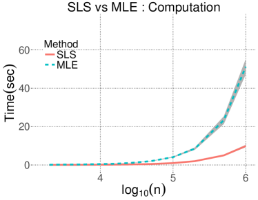
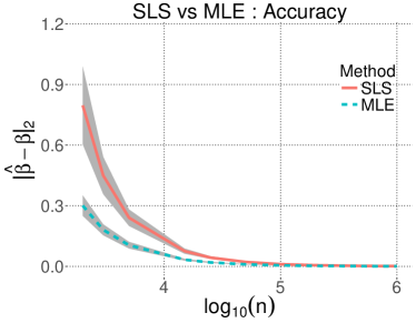
Figure 1: Logistic regression with iid standard Gaussian design. The left plot shows the computational cost (time) for finding the MLE and SLS as $n$ grows and $p=200$. The right plot depicts the accuracy of the estimators. In the regime where the MLE is expensive to compute, the SLS is found much more rapidly and has the same accuracy. R’s built-in functions are used to find the MLE.

The second step of Algorithm 1 involves solving a simple root-finding problem. As with the first step of the algorithm, there are numerous methods available for completing this task. Newton’s root-finding method with quadratic convergence or Halley’s method with cubic convergence may be appropriate choices. We highlight that this step costs only $\mathcal{O}\left(n\right)$ per-iteration and that we can attain up to a cubic rate of convergence. The resulting per-iteration cost is cheaper than other commonly used batch algorithms by at least a factor of $\mathcal{O}\left(p\right)$ — indeed, the cost of computing the gradient is $\mathcal{O}\left(np\right)$. For simplicity, we use Newton’s root-finding method.

Correct initialization of the scaling constant $c$ depends on the optimization problem. For example, in the case of GLM problems, assuming that the GLM is a good approximation to the true conditional distribution, by the law of total variance and basic properties of GLMs, we have

$$\mathrm{Var}\left(y_{i}\right)=\mathbb{E}\left[\mathrm{Var}\left(y_{i}\mid x_{i}\right)\right]+\mathrm{Var}\left(\mathbb{E}\left[y_{i}\mid x_{i}\right]\right)\approx c_{\Psi}^{-1}+\text{Var}\big{(}{\Psi^{(1)}}({\langle x_{i},\beta\rangle})\big{)}.$$ (4.1)

It follows that the initialization $c=2/\mathrm{Var}\left(y_{i}\right)$ is reasonable as long as $c_{\Psi}^{-1}\approx\mathbb{E}\left[\mathrm{Var}\left(y_{i}\mid x_{i}\right)\right]$ is not much smaller than $\text{Var}\big{(}{\Psi^{(1)}}({\langle x_{i},\beta\rangle})\big{)}$. Our experiments show that SLS is very robust to initialization.

In Figure 1, we compare the performance of our SLS estimator to that of the MLE in a GLM optimization problem, when both are used to analyze synthetic data generated from a logistic regression model under general Gaussian design with randomly generated covariance matrix. The left plot shows the computational cost of obtaining both estimators as $n$ increases for fixed $p$. The right plot shows the accuracy of the estimators. In the regime $n\gg p\gg 1$ — where the MLE is hard to compute — the MLE and the SLS achieve the same accuracy, yet SLS has significantly smaller computation time. We refer the reader to Section 5 for theoretical results characterizing the finite sample behavior of the SLS.

5 Theoretical results

In this section, we use the zero-bias transformations [GR97] to generalize the equivalence relation given in the previous section to the settings where the covariates are non-Gaussian.

Definition 1.

Let $z$ be a random variable with mean 0 and variance $\sigma^{2}$. Then, there exists a random variable $z^{*}$ that satisfies $\mathbb{E}\left[zf(z)\right]=\sigma^{2}\mathbb{E}[f^{(1)}(z^{*})],$  for all differentiable functions $f$. The distribution of $z^{*}$ is said to be the $z$-zero-bias distribution.

The existence of $z^{*}$ in Definition 1 is a consequence of Riesz representation theorem [GR97]. The normal distribution is the unique distribution whose zero-bias transformation is itself (i.e. the normal distribution is a fixed point of the operation mapping the distribution of $z$ to that of $z^{*}$ – which is basically Stein’s lemma).

To provide some intuition behind the usefulness of the zero-bias transformation, we refer back to the proof of Proposition 3.1. For simplicity, assume that the covariate vector $x_{i}$ has iid entries with mean 0, and variance 1. Then the zero-bias transformation applied to the $j$-th normal equation in (3.3) yields

$$\underbrace{\mathbb{E}\left[y_{i}x_{ij}\right]=\mathbb{E}\left[x_{ij}{\Psi^{(1)}}\big{(}x_{ij}\beta_{j}+\Sigma_{k\neq j}x_{ik}\beta_{k}\big{)}\right]}_{\text{$j$-th normal equation}}=\underbrace{\beta_{j}\mathbb{E}\left[{\Psi^{(2)}}\left(x_{ij}^{*}\beta_{j}+\Sigma_{k\neq j}x_{ik}\beta_{ik}\right)\right]}_{\text{Zero-bias transformation}}.$$ (5.1)

The distribution of $x_{ij}^{*}$ is the $x_{ij}$-zero-bias distribution and is entirely determined by the distribution of $x_{ij}$; general properties of $x_{ij}^{*}$ can be found, for example, in [CGS10]. If $\beta$ is well spread, it turns out that taken together, with $j=1,\ldots,p$, the far right-hand side in (5.1) behaves similar to the right side of (3.4), with ${\boldsymbol{\Sigma}}=\mathbb{I}$; that is, the behavior is similar to the Gaussian case, where the proportionality relationship given in Proposition 3.1 holds. This argument leads to an approximate proportionality relationship for problems with non-Gaussian predictors, which, when carried out rigorously, yields the following result.

Theorem 5.1.

Suppose that the whitened covariates $w_{i}={\boldsymbol{\Sigma}}^{-\nicefrac{{1}}{{2}}}x_{i}$ are independent with mean 0, covariance $\mathbb{I}$, and have sub-Gaussian norm bounded by $\kappa$. Furthermore, $w_{i}$’s have constant first and second conditional moments, i.e., $\forall j\in[p]$ and $\tilde{\beta}={\boldsymbol{\Sigma}}^{\nicefrac{{1}}{{2}}}\beta^{\sf pop}$, $\mathbb{E}[{w_{ij}\big{|}\Sigma_{k\neq j}\tilde{\beta}_{k}w_{ik}}]$ and $\mathbb{E}[{w_{ij}^{2}\big{|}\Sigma_{k\neq j}\tilde{\beta}_{k}w_{ik}}]$ are constant. Let $\|\beta^{\sf pop}\|_{2}=\tau$ and assume $\beta^{\sf pop}$ is $r$-well-spread in the sense that $\tau/\left\|\beta^{\sf pop}\right\|_{\infty}=r\sqrt{p}$ for some $r\in(0,1]$, and the function ${\Psi^{(2)}}$ is Lipschitz continuous with constant $k$. Then, for $c_{\Psi}=1/\mathbb{E}\left[{\Psi^{(2)}}({\langle x_{i},\beta^{\sf pop}\rangle})\right]$, and $\rho=\rho_{\infty}({\boldsymbol{\Sigma}}^{1/2})$ denoting the condition number of ${\boldsymbol{\Sigma}}^{1/2}$, we have

$$\left\|\frac{1}{c_{\Psi}}\times\beta^{\sf pop}-\beta^{\sf ols}\right\|_{\infty}\leq\frac{\eta}{p},\ \text{ where }\ \eta=8k\kappa^{3}\rho\|{\boldsymbol{\Sigma}}^{1/2}\|_{\infty}(\tau/r)^{2}.$$ (5.2)

Theorem 5.1 is proved in the Appendix. It implies that the population parameters $\beta^{\sf ols}$ and $\beta^{\sf pop}$ are approximately equivalent up to a scaling factor, with an error bound of $\mathcal{O}\left(1/p\right)$. The assumption that $\beta^{\sf pop}$ is well-spread can be relaxed with minor modifications. For example, if we have a sparse coefficient vector, where $\mathrm{supp}(\beta^{\sf pop})=\{j;\ \beta^{\sf pop}_{j}\neq 0\}$ is the support set of $\beta^{\sf pop}$, then Theorem 5.1 holds with $p$ replaced by the size of the support set.

The assumptions on the conditional moments are the relaxed versions of assumptions that are commonly encountered in dimension reduction techniques. For example, sliced inverse regression methods assume that the first conditional moment $\mathbb{E}\left[x\big{|}{\langle x,\beta\rangle}\right]$ is linear in $x$ for all $\beta$ [LD89, Li91], which is satisfied by elliptically distributed random vectors. An important case that is not covered by these methods is the independent coordinate case, i.e., when the whitened covariates have independent, but not necessarily identical entries. It is straightforward to observe that this case satisfies the assumptions of Theorem 5.1. We refer reader to [LD09], for a good review of dimension reduction techniques and their corresponding assumptions. We also highlight that our moment assumptions can be relaxed further, at the expense of introducing some additional complexity into the results.

An interesting consequence of Theorem 5.1 and the remarks following the theorem is that whenever an entry of $\beta^{\sf pop}$ is zero, the corresponding entry of $\beta^{\sf ols}$ has to be small, and conversely. For $\lambda\geq 0$, define the lasso coefficients

$${\beta}^{\sf lasso}_{\lambda}=\operatorname{argmin}\displaylimits_{\beta\in{\mathbb{R}}^{p}}\ \frac{1}{2}\mathbb{E}\left[(y_{i}-{\langle x_{i},\beta\rangle})^{2}\right]+\lambda\left\|\beta\right\|_{1}.$$ (5.3)

Corollary 5.2.

For any $\lambda\geq\eta/|\mathrm{supp}(\beta^{\sf pop})|$, if $\mathbb{E}\left[x_{i}\right]=0$ and $\mathbb{E}\left[x_{i}x_{i}^{T}\right]=\mathbb{I}$, we have $\mathrm{supp}({\beta}^{\sf lasso})\subset\mathrm{supp}(\beta^{\sf pop}).$ Further, if $\lambda$ and $\beta^{\sf pop}$ also satisfy that $\forall j\in\mathrm{supp}(\beta^{\sf pop})$, $|\beta^{\sf pop}_{j}|>c_{\Psi}\left(\lambda+\eta/|\mathrm{supp}(\beta^{\sf pop})|\right)$, then we have $\mathrm{supp}({\beta}^{\sf lasso})=\mathrm{supp}(\beta^{\sf pop}).$

So far in this section, we have only discussed properties of the population parameters, such as $\beta^{\sf pop}$ and $\beta^{\sf ols}$. In the remainder of this section, we turn our attention to results for the estimators that are the main focus of this paper; these results ultimately build on our earlier results, i.e. Theorem 5.1.

In order to precisely describe the performance of $\hat{\beta}^{\sf\hskip 0.72229ptsls}$, we first need bounds on the OLS estimator. The OLS estimator has been studied extensively in the literature; however, for our purposes, we find it convenient to derive a new bound on its accuracy. While we have not seen this exact bound elsewhere, it is very similar to Theorem 5 of [DLFU13].

Proposition 5.3.

Assume that $\mathbb{E}\left[x_{i}\right]=0$, $\mathbb{E}\left[x_{i}x_{i}^{T}\right]={\boldsymbol{\Sigma}}$, and that ${\boldsymbol{\Sigma}}^{-\nicefrac{{1}}{{2}}}x_{i}$ and $y_{i}$ are sub-Gaussian with norms $\kappa$ and $\gamma$, respectively. For $\lambda_{\text{min}}$ denoting the smallest eigenvalue of ${\boldsymbol{\Sigma}}$, and $|S|>\eta p$,

$$\left\|\hat{\beta}^{\sf ols}-\beta^{\sf ols}\right\|_{2}\leq\eta\lambda_{\text{min}}^{\scalebox{0.8}{ $-\nicefrac{{1}}{{2}}$}}\sqrt{\frac{p}{|S|}},$$ (5.4)

with probability at least $1-3e^{-p}$, where $\eta$ depends only on $\gamma$ and $\kappa$.

Proposition 5.3 is proved in the Supplementary Material. Our main result on the performance of $\hat{\beta}^{\sf\hskip 0.72229ptsls}$ is given next.

Theorem 5.4.

Let the assumptions of Theorem 5.1 and Proposition 5.3 hold with $\mathbb{E}[\|{\boldsymbol{\Sigma}}^{-\nicefrac{{1}}{{2}}}x\|_{2}]=\tilde{\mu}\sqrt{p}$. Further assume that the function $f(z)=z\mathbb{E}\left[{\Psi^{(2)}}({\langle x,\beta^{\sf ols}\rangle}z)\right]$ satisfies $f(\bar{c})>1+\bar{\delta}\sqrt{p}$ for some $\bar{c}$ and $\bar{\delta}$ such that the derivative of $f$ in the interval $[0,\bar{c}]$ does not change sign, i.e., its absolute value is lower bounded by $\upsilon>0$. Then, for $n$ and $|S|$ sufficiently large, with probability at least $1-5e^{-p}$, we have

$$\left\|\hat{\beta}^{\sf\hskip 0.72229ptsls}-\beta^{\sf pop}\right\|_{\infty}\leq\eta_{1}\frac{1}{p}+\eta_{2}\sqrt{\frac{p}{\min\left\{n/\log(n),|S|\right\}}},$$ (5.5)

where the constants $\eta_{1}$ and $\eta_{2}$ are defined by

$$\eta_{1}= \eta k\bar{c}\kappa^{3}\rho\|{\boldsymbol{\Sigma}}^{1/2}\|_{\infty}(\tau/r)^{2}$$ (5.6)

$$\eta_{2}= \eta\bar{c}\lambda_{\text{min}}^{-1/2}\left(1+\upsilon^{-1}\lambda_{\text{min}}^{1/2}\|\beta^{\sf ols}\|_{\infty}\max\left\{(b+k/\tilde{\mu}),k\bar{c}\kappa\right\}\right),$$ (5.7)

and $\eta>0$ is a constant depending on $\kappa$ and $\gamma$.

Note that the convergence rate of the upper bound in (5.5) depends on the sum of the two terms, both of which are functions of the data dimensions $n$ and $p$. The first term on the right in (5.5) comes from Theorem 5.1, which bounds the discrepancy between $c_{\Psi}\times\beta^{\sf ols}$ and $\beta^{\sf pop}$. This term is small when $p$ is large, and it does not depend on the number of observations $n$.

The second term in the upper bound (5.5) comes from estimating $\beta^{\sf ols}$ and $c_{\Psi}$. This term is increasing in $p$, which reflects the fact that estimating $\beta^{\sf pop}$ is more challenging when $p$ is large. As expected, this term is decreasing in $n$ and $|S|$, i.e. larger sample size yields better estimates. When the full OLS solution is used ($|S|=n$), the second term becomes $\mathcal{O}(\sqrt{p\log(n)/n})$, which suggests that $n/\log(n)$ should be at least of order $p$ for good performance. Also, note that there is a theoretical threshold for the sub-sampling size $|S|$, namely $\mathcal{O}\left(n/\log(n)\right)$, beyond which further sub-sampling provides no improvement. This suggests that the sub-sampling size should be smaller than $\mathcal{O}\left(n/\log(n)\right)$.

6 Converting One GLM to Another by Scaling

In this section, we describe an efficient algorithm to transform a generalized linear model to another. It is often the case that a practitioner would like to change the loss function (equivalently the model) he/she uses based on its performance. When the dataset is large, training a new model from the scratch is computationally inefficient and will be time consuming. In the following, we will use the proportionality relation to transition between different loss functions.

Assume that a practitioner fitted a GLM using the loss function (or cumulant generating function) $\Psi_{1}$, but he/she would like to train a new model using the loss function $\Psi_{2}$. Instead of maximizing the log-likelihood based on $\Psi_{2}$, one can exploit the proportionality relation and obtain the coefficients for the new GLM problem.

Algorithm 2 Conversion from one GLM to another

  Input: Data $(y_{i},x_{i})_{i=1}^{n}$, and $\hat{\beta}^{\text{glm}}_{1}$

  Step 1. Compute $\hat{y}=\mathbb{X}\hat{\beta}^{\text{glm}}_{1}$, and $\kappa=\frac{1}{n}\sum_{i=1}^{n}\Psi_{1}^{(2)}(\hat{y}_{i})$.

  Step 2. Solve the following equation for $\rho\in{\mathbb{R}}$: $\kappa=\frac{\rho}{n}\sum_{i=1}^{n}\Psi_{2}^{(2)}(\hat{y}_{i}\rho)$

            Use Newton’s root-finding method:

                  Initialize $\rho=1$;

                  Repeat until convergence:

                    $\rho\leftarrow\rho-\cfrac{\rho\,\frac{1}{n}\sum_{i=1}^{n}\Psi_{2}^{(2)}(\rho\,\hat{y}_{i})-\kappa}{\frac{1}{n}\sum_{i=1}^{n}\left\{\Psi_{2}^{(2)}(\rho\,\hat{y}_{i})+\rho\,\hat{y}_{i}\Psi_{2}^{(3)}(\rho\,\hat{y}_{i})\right\}}$.

              

  Output: $\hat{\beta}^{\text{glm}}_{2}=\rho\times\hat{\beta}^{\text{glm}}_{1}$.

Denote by $\beta^{\sf pop}_{1}$ and $\beta^{\sf pop}_{2}$ the GLM coefficients corresponding to the loss functions $\Psi_{1}$ and $\Psi_{2}$, respectively. We have

$$\frac{1}{c_{\Psi_{1}}}\beta^{\sf pop}_{1}=\frac{1}{c_{\Psi_{2}}}\beta^{\sf pop}_{2}=\beta^{\sf ols},$$

that is, both coefficients are proportional to the OLS coefficients which does not depend on the loss function. Therefore, these coefficients $\beta^{\sf pop}_{1}$ and $\beta^{\sf pop}_{2}$ are also proportional to each other and we can write

$$\beta^{\sf pop}_{2}=\frac{c_{\Psi_{2}}}{c_{\Psi_{1}}}\ \beta^{\sf pop}_{1}\coloneqq\rho\ \beta^{\sf pop}_{1},$$ (6.1)

where the proportionality constant between two GLM types turns out to be the ratio between $c_{\Psi_{1}}$ and $c_{\Psi_{2}}$, i.e. $\rho=c_{\Psi_{2}}/c_{\Psi_{1}}$. Using the definition of $c_{\Psi_{2}}$, we write

$$1 =c_{\Psi_{2}}\ \mathbb{E}\left[\Psi_{2}^{(2)}({\langle x,\beta^{\sf pop}_{2}\rangle})\right],$$

$$=c_{\Psi_{1}}\rho\ \mathbb{E}\left[\Psi_{2}^{(2)}({\langle x,\beta^{\sf pop}_{1}\rangle}\rho)\right].$$

Dividing the both sides by $c_{\Psi_{1}}$ and using the equality $1/c_{\Psi_{1}}=\mathbb{E}\left[\Psi_{1}^{(2)}({\langle x,\beta^{\sf pop}_{1}\rangle})\right]$, we obtain

$$\mathbb{E}\left[\Psi_{1}^{(2)}({\langle x,\beta^{\sf pop}_{1}\rangle})\right]=\rho\ \mathbb{E}\left[\Psi_{2}^{(2)}({\langle x,\beta^{\sf pop}_{1}\rangle}\rho)\right].$$

The above equation only involves $\beta^{\sf pop}_{1}$ as the coefficients (which is already assumed to be known or fitted by the practitioner). Therefore, if we solve it for the ratio $\rho$, we can estimate $\beta^{\sf pop}_{2}$ by simply using the proportionality relation given in (6.1).

The procedure described above is summarized as Algorithm 2. We emphasize that this procedure does not require the computation of the OLS estimator which was the main cost of SLS. The procedure only requires a per-iteration cost of $\mathcal{O}\left(n\right)$. In other words, conversion from one GLM type to another is much simpler than obtaining the GLM coefficients from the scratch.

7 Binary Classification with Proper Scoring Rules

In this section, we assume that for $i\in[n]$, the response is binary $y_{i}\ \in\{0,1\}$. The binary classification problem can be described by the following minimization of an empirical risk

$$\underset{\beta\in{\mathbb{R}}^{p}}{\text{minimize}}\ \frac{1}{n}\sum_{i=1}^{n}\ell(y_{i};q({\langle x_{i},\beta\rangle})),$$ (7.1)

where $\ell$ and $q$ are referred to as the loss and the link functions, respectively. There are various loss functions that are used in practice. Examples include log-loss, boosting loss, square loss etc (See Table 1). As before, we constrain our analysis on the canonical links. The concept of canonical links for binary classification is introduced by [BSS05], and it is quite similar to the generalized linear problems.

Table 1: Common loss functions and their canonical links

Name	Loss function: $\ell(y;q)$	Weight: $w(q)$	Canonical link: $q(z)$
Log-loss	$-y\log(q)-(1-y)\log(1-q)$	$\frac{1}{q(1-q)}$	$\frac{1}{1+\exp(-z)}$
Boosting loss	$y(q^{-1}-1)^{1/2}+(1-y)(q^{-1}-1)^{-1/2}$	$\frac{1}{[q(1-q)]^{3/2}}$	$\frac{1}{2}+\frac{z/2}{2(z^{2}/4+1)^{1/2}}$
Square loss	$y(1-q)^{2}+(1-y)q^{2}$	$1$	$\frac{1+z}{2}$

For any given loss function, we define the partial losses $\ell_{k}(\cdot)=\ell(y=k;\cdot)$ for $k\in\{0,1\}$. Since we have a binary response variable, we can write any loss in the following format

$$\ell(y;q)= y\ell_{1}(q)+(1-y)\ell_{0}(q),$$

$$= y\left(\ell_{1}(q)-\ell_{0}(q)\right)+\ell_{0}(q).$$

The above formulation is of the form of a generalized linear problem. Before moving forward, we recall the concept of proper scoring in binary classification, which is sometimes referred to as Fisher consistency.

Definition 2 (Proper scoring rules).

Assume that $y\sim\text{Bernoulli}(\eta)$. If the expected loss $\mathbb{E}\left[\ell(y,q)\right]$ is minimized by $q=\eta$ for all $\eta\in(0,1)$, we call the loss function a proper scoring rule.

The following theorem by [Sch89] provides a methodology for constructing a loss function for the proper scoring rules.

Theorem 7.1 ([Sch89]).

Let $w(dt)$ be a positive measure on $(0,1)$ that is finite on interval $({\epsilon},1-{\epsilon})$ $\forall{\epsilon}>0$. Then the following defines a proper scoring rule

$$\ell_{1}(q)=\int^{1}_{q}(1-t)w(dt),\text{ and }\ell_{0}(q)=\int^{q}_{0}tw(dt).$$

The measure $w(dt)$ uniquely defines the loss function (generally referred to as the weight function, since all losses can be written as weighted average of cost weighted misclassification error [BSS05, RW10]). Examples of weight functions is given in Table 1. The above theorem has many interesting interpretations; one that is most useful to us is that $\ell_{0}^{(1)}(q)=qw(q)$.

The notion of canonical links for proper scoring rules are introduced by [BSS05], which corresponds to the notion of matching loss [HKW99, RW10]. The derivation of canonical links stems from the Hessian of the above minimization, which remedies two potential problems: non-convexity and asymptotic variance inflation. It turns out that by setting $w(q)q^{(1)}$ as constant, one can remedy both problems [BSS05]. We will skip the derivation and, without loss of generality, assume that the canonical link-loss pair satisfies $w(q)q^{(1)}=1$. Note that any loss function has a natural canonical link. The following Theorem summarizes this concept.

Theorem 7.2 ([BSS05]).

For proper scoring rules with $w>0$, there exists a canonical link function which is unique up to addition and multiplication by constants. Conversely, any link function is canonical for a unique proper scoring rule.

The canonical link for a given loss function can be explicitly derived from the equation $w(q)q^{(1)}=1$. We have provided some examples in Table 1. Using the definition of canonical link for proper scoring rules, we write the normal equations $\frac{\mathrm{d}}{\mathrm{d}\beta}\mathbb{E}\left[\ell(y,q({\langle x,\beta\rangle}))\right]=0$ as

$$\mathbb{E}\left[xq^{(1)}({\langle x,\beta\rangle})\ell_{0}^{(1)}(q({\langle x,\beta\rangle}))\right]= \mathbb{E}\left[yxq^{(1)}({\langle x,\beta\rangle})\left(\ell_{0}^{(1)}(q({\langle x,\beta\rangle}))-\ell_{1}^{(1)}(q({\langle x,\beta\rangle}))\right)\right],$$

$$\mathbb{E}\left[xq^{(1)}({\langle x,\beta\rangle})q({\langle x,\beta\rangle})w(q({\langle x,\beta\rangle}))\right]= \mathbb{E}\left[yq^{(1)}({\langle x,\beta\rangle})w(q({\langle x,\beta\rangle}))\right],$$

$$\mathbb{E}\left[xq({\langle x,\beta\rangle})\right]= \mathbb{E}\left[yx\right],$$

$${\boldsymbol{\Sigma}}\beta\mathbb{E}\left[q^{(1)}({\langle x,\beta\rangle})\right]= \mathbb{E}\left[yx\right].$$

The last equation provides us with the analog of the proportionality relation we observed in generalized linear problems. In this case, we observe that the proportionality constant becomes $1/\mathbb{E}\left[q^{(1)}({\langle x,\beta\rangle})\right]$. Therefore, our algorithm can be used to obtain a fast training procedure for the binary classification problems under canonical links.

8 Canonicalization of the Square Loss

In this section, we present a method to approximate the square loss with a canonical form. Using this canonical approximation, we can use the techniques developed in previous sections to gain computational benefits. Consider a minimization problem of the following form

$$\underset{\beta}{\text{minimize}}\ \frac{1}{n}\sum_{i=1}^{n}[y_{i}-f({\langle x_{i},\beta\rangle})]^{2}.$$ (8.1)

The above problem is commonly encountered in many machine learning tasks – specifically, in the context of neural networks, the function $f$ is called the activation function. Here, we consider a toy example to demonstrate how our methodology can be useful in a minimization problem of the above form.

We first use Taylor series expansion around a point $\theta$ (which should be close to ${\langle x,\beta\rangle}$), in order to approximate the function $f(z)$ with a linear function around $f(\theta)$. This way, the square loss can be approximated with a generalized linear loss. We write

$$\min_{\beta}(y-f({\langle x,\beta\rangle}))^{2} =\min_{\beta}f({\langle x,\beta\rangle})^{2}-2yf({\langle x,\beta\rangle})$$ (8.2)

$$\approx\min_{\beta}\frac{f({\langle x,\beta\rangle})^{2}}{2f^{\prime}(\theta)}-y{\langle x,\beta\rangle}.$$

Then, we would have

$$\Psi(z)=\frac{f(z)^{2}}{2f^{\prime}(\theta)},$$ (8.3)

and the proportionality relation given in previous sections would hold approximately. The above approximation will be accurate when the activation function is smooth around the user-specified point $\theta$. We suggest to use $\theta=0$ since when $p$ is large and $\beta$ is well-spread, the inner product ${\langle x,\beta\rangle}$ should be close to its expectation $\mathbb{E}\left[{\langle x,\beta\rangle}\right]=0$. This method can be used to derive proportionality relations for GLMs with non-canonical links (conditional on link being nice), and also may be of interest in non-convex optimization.

9 Experiments

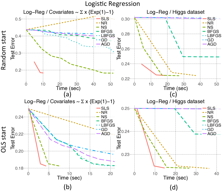
Figure 2: We compared the performance of SLS to that of MLE for the logistic regression problem on several datasets. MLE optimization is solved by various optimization algorithms. SLS is represented with red straight line. The details are provided in Table 2.

This section contains the results of a variety of numerical studies, which show that the Scaled Least Squares estimator reaches the minimum achievable test error substantially faster than commonly used batch algorithms for finding the MLE. Both logistic and Poisson regression models (two types of GLMs) are utilized in our analyses, which are based on several synthetic and real datasets.

Below, we briefly describe the optimization algorithms for the MLE that were used in the experiments.

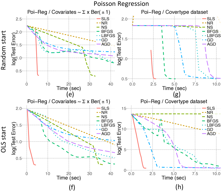
Figure 3: We compared the performance of SLS to that of MLE for the Poisson regression problem on several datasets. MLE optimization is solved by various optimization algorithms. SLS is represented with red straight line. The details are provided in Table 2.

1. Newton-Raphson (NR) achieves locally quadratic convergence by scaling the gradient by the inverse of the Hessian evaluated at the current iterate. Computing the Hessian has a per-iteration cost of $\mathcal{O}\left(np^{2}\right)$, which makes it impractical for large-scale datasets.

2. Newton-Stein (NS) is a recently proposed second-order batch algorithm specifically designed for GLMs [Erd15a, Erd15b]. The algorithm uses Stein’s lemma and sub-sampling to efficiently estimate the Hessian with a cost of $\mathcal{O}\left(np\right)$ per-iteration, achieving near quadratic rates.

3. Broyden-Fletcher-Goldfarb-Shanno (BFGS) is the most popular and stable quasi-Newton method [Nes04]. At each iteration, the gradient is scaled by a matrix that is formed by accumulating information from previous iterations and gradient computations. The convergence is locally super-linear with a per-iteration cost of $\mathcal{O}\left(np\right)$.

4. Limited memory BFGS (LBFGS) is a variant of BFGS, which uses only the recent iterates and gradients to approximate the Hessian, providing significant improvement in terms of memory usage. LBFGS has many variants; we use the formulation given in [Bis95].

5. Gradient descent (GD) takes a step in the opposite direction of the gradient, evaluated at the current iterate. Its performance strongly depends on the condition number of the design matrix. Under certain assumptions, the convergence is linear with $\mathcal{O}\left(np\right)$ per-iteration cost.

6. Accelerated gradient descent (AGD) is a modified version of gradient descent with an additional “momentum” term [Nes83]. Its per iteration cost is $\mathcal{O}\left(np\right)$ and its performance strongly depends on the smoothness of the objective function.

For all the algorithms for computing the MLE, the step size at each iteration is chosen via the backtracking line search [BV04].

Recall that the proposed Algorithm 1 is composed of two steps; the first finds an estimate of the OLS coefficients. This up-front computation is not needed for any of the MLE algorithms described above. On the other hand, each of the MLE algorithms requires some initial value for $\beta$, but no such initialization is needed to find the OLS estimator in Algorithm 1. This raises the question of how the MLE algorithms should be initialized, in order to compare them fairly with the proposed method. We consider two scenarios in our experiments: first, we use the OLS estimator computed for Algorithm 1 to initialize the MLE algorithms; second, we use a random initial value.

On each dataset, the main criterion for assessing the performance of the estimators is how rapidly the minimum test error is achieved. The test error is measured as the mean squared error of the estimated mean using the current parameters at each iteration on a test dataset, which is a randomly selected (and set-aside) 10% portion of the entire dataset. As noted previously, the MLE is more accurate for small $n$ (see Figure 1). However, in the regime considered here ($n\gg p\gg 1$), the MLE and the SLS perform very similarly in terms of their error rates; for instance, on the Higgs dataset, the SLS and MLE have test error rates of $22.40\%$ and $22.38\%$, respectively. For each dataset, the minimum achievable test error is set to be the maximum of the final test errors, where the maximum is taken over all of the estimation methods. Let ${\boldsymbol{\Sigma}}^{(1)}$ and ${\boldsymbol{\Sigma}}^{(2)}$ be two randomly generated covariance matrices. The datasets we analyzed were: (i) a synthetic dataset generated from a logistic regression model with iid $\{\mbox{exponential}(1)\!-\!1\}$ predictors scaled by ${\boldsymbol{\Sigma}}^{(1)}$; (ii) the Higgs dataset (logistic regression) [BSW14]; (iii) a synthetic dataset generated from a Poisson regression model with iid binary($\pm 1$) predictors scaled by ${\boldsymbol{\Sigma}}^{(2)}$; (iv) the Covertype dataset (Poisson regression) [BD99].

In all cases, the SLS outperformed the alternative algorithms for finding the MLE by a large margin, in terms of computation. Detailed results may be found in Figures 2 and 3, and Table 2. We provide additional experiments with different datasets in the Supplementary Material.

Table 2: Details of the experiments shown in Figures 2 and 3.

Model	Logistic regression				Poisson regression
Dataset	${\boldsymbol{\Sigma}}\times${Exp(1)-1}		Higgs [BSW14]		${\boldsymbol{\Sigma}}\times$Ber($\pm 1$)		Covertype [BD99]
Size	$n=6.0\times 10^{5}$, $p=300$		$n=1.1\!\times\!10^{7}$, $p=29$		$\!n=6.0\!\times\!10^{5}$, $p=300$​		$\!n=5.8\!\times\!10^{5}$, $p=53$​​​​
Initialized​​​​	Rnd	Ols	Rnd	Ols	Rnd	Ols	Rnd	Ols
Plot​	(a)	(b)	(c)	(d)	(e)	(f)	(g)	(h)
Method	Time in seconds / number of iterations  (to reach min test error)
Sls	8.34/4	2.94/3	13.18/3	9.57/3	5.42/5	3.96/5	2.71/6	1.66/20
Nr	301.06/6	82.57/3	37.77/3	36.37/3	170.28/5	130.1/4	16.7/8	32.48/18
Ns	51.69/8	7.8/3	27.11/4	26.69/4	32.71/5	36.82/4	21.17/10	​​282.1/216​​​​
Bfgs	148.43/31	24.79/8	660.92/68	701.9/68	67.24/29	72.42/26	5.12/7	22.74/59
Lbfgs	125.33/39	24.61/8	​​6368.1/651​​	​​6946.1/670​​	​224.6/106​	​​357.1/88​​	10.01/14	10.05/17
Gd	669/138	134.91/25	​​​100871/10101​​​​	​​​141736/13808​​​​	1711/513	​​1364/374​​	14.35/25	33.58/87
Agd	218.1/61	35.97/12	​​ 2405.5/251​​	​​2879.69/277​​	103.3/51	​​102.74/40​​	11.28/15	11.95/25

10 Discussion

In this paper, we showed that the true minimizer of a generalized linear problem and the OLS estimator are approximately proportional under the general random design setting. Using this relation, we proposed a computationally efficient algorithm for large-scale problems that achieves the same accuracy as the empirical risk minimizer by first estimating the OLS coefficients and then estimating the proportionality constant through iterations that can attain quadratic or cubic convergence rate, with only $\mathcal{O}\left(n\right)$ per-iteration cost.

We briefly mentioned that the proportionality between the coefficients holds even when there is regularization in Section 3.1. Further pursuing this idea may be interesting for large-scale problems where regularization is crucial. Another interesting line of research is to find similar proportionality relations between the parameters in other large-scale optimization problems such as support vector machines. Such relations may reduce the problem complexity significantly.

Appendix A Proof of Main Results

In this section, we provide the details and the proofs of our technical results. For convenience, we briefly state the following definitions.

Definition 3 (Sub-Gaussian).

For a given constant $\kappa$, a random variable $x\in{\mathbb{R}}$ is said to be sub-Gaussian if it satisfies

$$\sup_{m\geq 1}m^{\nicefrac{{-1}}{{2}}}\mathbb{E}\left[|x|^{m}\right]^{1/m}\leq\kappa.$$

Smallest such $\kappa$ is the sub-Gaussian norm of $x$ and it is denoted by $\|x\|_{\psi_{2}}$. Similarly, a random vector $y\in{\mathbb{R}}^{p}$ is a sub-Gaussian vector if there exists a constant $\kappa^{\prime}$ such that

$$\sup_{v\in S^{p-1}}\|\langle y,v\rangle\|_{\psi_{2}}\leq\kappa^{\prime}.$$

Definition 4 (Sub-exponential).

For a given constant $\kappa$, a random variable $x\in{\mathbb{R}}$ is called sub-exponential if it satisfies

$$\sup_{m\geq 1}m^{-1}\mathbb{E}\left[|x|^{m}\right]^{1/m}\leq\kappa.$$

Smallest such $\kappa$ is the sub-exponential norm of $x$ and it is denoted by $\|x\|_{\psi_{1}}$. Similarly, a random vector $y\in{\mathbb{R}}^{p}$ is a sub-exponential vector if there exists a constant $\kappa^{\prime}$ such that

$$\sup_{v\in S^{p-1}}\|\langle y,v\rangle\|_{\psi_{1}}\leq\kappa^{\prime}.$$

We start with the proof of Theorem 5.1.

Proof of Theorem 5.1.

For simplicity, we denote the whitened covariate by $w={\boldsymbol{\Sigma}}^{-1/2}x$. Since $w$ is sub-Gaussian with norm $\kappa$, its $j$-th entry $w_{j}$ has bounded third moment. That is,

$$\kappa= \sup_{\left\|u\right\|_{2}=1}\left\|{\langle u,w\rangle}\right\|_{\psi_{2}},$$ (A.1)

$$\geq \left\|w_{j}\right\|_{\psi_{2}}=\sup_{m\geq 1}m^{-1/2}\mathbb{E}\left[|w_{j}|^{m}\right]^{1/m},$$

$$\geq \frac{1}{\sqrt{3}}\mathbb{E}\left[|w_{j}|^{3}\right]^{1/3},$$

where in the first step, we used $u=e_{j}$, the $j$-th standard basis vector. Hence, we obtain a bound on the third moment, i.e,

$$\max_{j}\mathbb{E}\left[|w_{j}|^{3}\right]\leq 3^{3/2}\kappa^{3}.$$ (A.2)

Using the normal equations, we write

$$\mathbb{E}\left[yx\right]=\mathbb{E}\left[x{\Psi^{(1)}}(\langle x,\beta\rangle)\right]= {\boldsymbol{\Sigma}}^{1/2}\mathbb{E}\left[w{\Psi^{(1)}}(\langle w,{\boldsymbol{\Sigma}}^{1/2}\beta\rangle)\right],$$ (A.3)

$$= {\boldsymbol{\Sigma}}^{1/2}\mathbb{E}\left[w{\Psi^{(1)}}(\langle w,\tilde{\beta}\rangle)\right],$$

where we defined $\tilde{\beta}={\boldsymbol{\Sigma}}^{1/2}\beta$. By multiplying both sides with ${\boldsymbol{\Sigma}}^{-1}$, we obtain

$$\beta^{\sf ols}={\boldsymbol{\Sigma}}^{-1/2}\mathbb{E}\left[w{\Psi^{(1)}}(\langle w,\tilde{\beta}\rangle)\right].$$ (A.4)

Now we define the partial sums $W_{-i}=\sum_{j\neq i}\tilde{\beta}_{j}w_{j}={\langle\tilde{\beta},w\rangle}-\tilde{\beta}_{i}w_{i}$. We will focus on the $i$-th entry of the above expectation given in (A.4). Denoting the zero biased transformation of $w_{i}$ conditioned on $W_{-i}$ by $w_{i}^{*}$, we have

$$\mathbb{E}\left[w_{i}{\Psi^{(1)}}(\langle w,\tilde{\beta}\rangle)\right]= \mathbb{E}\left[\mathbb{E}\left[w_{i}{\Psi^{(1)}}\left(\tilde{\beta}_{i}w_{i}+W_{-i}\right)\big{|}W_{-i}\right]\right],$$ (A.5)

$$= \tilde{\beta}_{i}\mathbb{E}\left[{\Psi^{(2)}}(\tilde{\beta}_{i}w_{i}^{*}+W_{-i})\right],$$

$$= \tilde{\beta}_{i}\mathbb{E}\left[{\Psi^{(2)}}(\tilde{\beta}_{i}(w_{i}^{*}-w_{i})+\langle w,\tilde{\beta}\rangle)\right],$$

where in the second step, we used the assumption on conditional moments. Let $\mathbf{D}$ be a diagonal matrix with diagonal entries $\mathbf{D}_{ii}=\mathbb{E}\left[{\Psi^{(2)}}(\tilde{\beta}_{i}(w_{i}^{*}-w_{i})+\langle w,\tilde{\beta}\rangle)\right]$. Using (A.4) together with (A.5), we obtain the equality

$$\beta^{\sf ols}= {\boldsymbol{\Sigma}}^{-1/2}\mathbf{D}\tilde{\beta},$$ (A.6)

$$= {\boldsymbol{\Sigma}}^{-1/2}\mathbf{D}{\boldsymbol{\Sigma}}^{1/2}\beta.$$

Now, using the Lipschitz continuity assumption of the variance function, we have

$$\left|\mathbb{E}\left[{\Psi^{(2)}}(\tilde{\beta}_{i}(w_{i}^{*}-w_{i})+\langle w,\tilde{\beta}\rangle)\right]-\mathbb{E}\left[{\Psi^{(2)}}(\langle w,\tilde{\beta}\rangle)\right]\right|\leq k|\tilde{\beta}_{i}|\mathbb{E}\left[|w_{i}^{*}-w_{i}|\right].$$ (A.7)

In the following, we will use the properties of zero-biased transformations. Consider the quantity

$$r=\sup\frac{\mathbb{E}\left[|w^{*}_{i}-w_{i}|\big{|}W_{-i}\right]}{\mathbb{E}\left[|w_{i}|^{3}\big{|}W_{-i}\right]}$$ (A.8)

where $w^{*}_{i}$ has $w_{i}$-zero biased distribution (conditioned on $W_{-i}$) and the supremum is taken with respect to all random variables with mean 0, standard deviation 1 and finite third moment, and $w^{*}_{i}$ is achieving the minimal $\ell_{1}$ coupling to $w_{i}$ conditioned on $W_{-i}$. It is shown in [Gol07] that the above bound holds for $r=1.5$ for the unconditional zero-bias transformations. Here, we take a similar approach to show that the same bound holds for the conditional case as well. By using the triangle inequality, we have

$$\mathbb{E}\left[|w^{*}_{i}-w_{i}|\big{|}W_{-i}\right]\leq \mathbb{E}\left[|w^{*}_{i}|\big{|}W_{-i}\right]+\mathbb{E}\left[|w_{i}|\big{|}W_{-i}\right]$$

$$\leq \frac{1}{2}\mathbb{E}\left[|w_{i}|^{3}\big{|}W_{-i}\right]+\mathbb{E}\left[|w_{i}|^{3}\big{|}W_{-i}\right]^{1/3}.$$

Since $\mathbb{E}\left[|w_{i}|^{2}\big{|}W_{-i}\right]$ is constant, it is equal to $\mathbb{E}\left[|w_{i}|^{2}\right]=1$. This yields that the second term in the last line is upper bounded by $\mathbb{E}\left[|w_{i}|^{3}\big{|}W_{-i}\right]$. Consequently, by taking expectations over both hand sides we obtain that

$$\mathbb{E}\left[|w^{*}_{i}-w_{i}|\right]\leq 1.5\ \mathbb{E}\left[|w_{i}|^{3}\right].$$

Then the right hand side of (A.7) can be upper bounded by

$$k|\tilde{\beta}_{i}|\mathbb{E}\left[|w_{i}^{*}-w_{i}|\right]\leq rk\max_{i}\left\{|\tilde{\beta}_{i}|\mathbb{E}\left[|w_{i}|^{3}\right]\right\},$$ (A.9)

$$\leq 1.5k\left\|{\boldsymbol{\Sigma}}^{1/2}\beta\right\|_{\infty}3^{3/2}\kappa^{3},$$

$$\leq 8k\kappa^{3}\|{\boldsymbol{\Sigma}}^{1/2}\beta\|_{\infty},$$

where in the second step we used the bound on the third moment given in (A.2). The last inequality provides us with the following result,

$$\max_{i}\left|\mathbf{D}_{ii}-\frac{1}{c_{\Psi}}\right|\leq 8k\kappa^{3}\|{\boldsymbol{\Sigma}}^{1/2}\beta\|_{\infty}.$$ (A.10)

Finally, combining this with (A.4) and (A.6), we obtain

$$\left\|\beta^{\sf ols}-\frac{1}{c_{\Psi}}\beta\right\|_{\infty}= \left\|{\boldsymbol{\Sigma}}^{-1/2}\mathbf{D}{\boldsymbol{\Sigma}}^{1/2}\beta-\frac{1}{c_{\Psi}}\beta\right\|_{\infty},$$ (A.11)

$$= \left\|{\boldsymbol{\Sigma}}^{-1/2}\left(\mathbf{D}-\frac{1}{c_{\Psi}}\mathbb{I}\right){\boldsymbol{\Sigma}}^{1/2}\beta\right\|_{\infty},$$

$$\leq \max_{i}\left|\mathbf{D}_{ii}-\frac{1}{c_{\Psi}}\right|\left\|{\boldsymbol{\Sigma}}^{1/2}\right\|_{\infty}\left\|{\boldsymbol{\Sigma}}^{-1/2}\right\|_{\infty}\left\|\beta\right\|_{\infty}^{2},$$

$$\leq 8k\kappa^{3}\rho({\boldsymbol{\Sigma}}^{1/2})\|{\boldsymbol{\Sigma}}^{1/2}\|_{\infty}\frac{\tau^{2}}{r^{2}p},$$

where in the last step, we used the assumption that $\beta$ is $r$-well-spread. ∎

Proof of Proposition 5.3.

For convenience, we denote the whitened covariates with $w_{i}={\boldsymbol{\Sigma}}^{-1/2}x_{i}$. We have $\mathbb{E}\left[w_{i}\right]=0$, $\mathbb{E}\left[w_{i}w_{i}^{T}\right]=\mathbb{I}$, and $\left\|w_{i}\right\|_{\psi_{2}}\leq\kappa$. Also denote the sub-sampled covariance matrix with $\widehat{\boldsymbol{\Sigma}}=\frac{1}{|S|}\sum_{i\in S}x_{i}x_{i}^{T}$, and its whitened version as $\widetilde{{\boldsymbol{\Sigma}}}=\frac{1}{|S|}\sum_{i\in S}w_{i}w_{i}^{T}$. Further, define $\hat{\zeta}=\frac{1}{n}\sum_{i=1}^{n}w_{i}y_{i}$ and $\zeta=\mathbb{E}\left[wy\right]$. Then, we have

$$\hat{\beta}^{\sf ols}=\widehat{\boldsymbol{\Sigma}}^{-1}{\boldsymbol{\Sigma}}^{1/2}\hat{\zeta}\ \ \text{ and }\ \ \beta^{\sf ols}={\boldsymbol{\Sigma}}^{-1/2}\zeta.$$

For now, we work on the event that $\widehat{\boldsymbol{\Sigma}}$ is invertible. We will see that this event holds with very high probability. We write

$$\left\|{\boldsymbol{\Sigma}}^{1/2}(\hat{\beta}^{\sf ols}-\beta^{\sf ols})\right\|_{2}= \left\|{\boldsymbol{\Sigma}}^{1/2}\widehat{\boldsymbol{\Sigma}}^{-1}{\boldsymbol{\Sigma}}^{1/2}\hat{\zeta}-{\boldsymbol{\Sigma}}^{-1/2}\zeta\right\|_{2},$$ (A.12)

$$= \left\|\widetilde{{\boldsymbol{\Sigma}}}^{-1}\left\{\hat{\zeta}-\zeta+\left(\mathbb{I}-{\boldsymbol{\Sigma}}^{-1/2}\widehat{\boldsymbol{\Sigma}}{\boldsymbol{\Sigma}}^{-1/2}\right)\zeta\right\}\right\|_{2},$$

$$\leq \left\|\widetilde{{\boldsymbol{\Sigma}}}^{-1}\right\|_{2}\left\{\left\|\hat{\zeta}-\zeta\right\|_{2}+\left\|\mathbb{I}-\widetilde{{\boldsymbol{\Sigma}}}\right\|_{2}\left\|\zeta\right\|_{2}\right\},$$

where we used the triangle inequality and the properties of the operator norm.

For the first term on the right hand side of (A.12), we write

$$\left\|\widetilde{{\boldsymbol{\Sigma}}}^{-1}\right\|_{2}= \frac{1}{\lambda_{\text{min}}(\widetilde{{\boldsymbol{\Sigma}}})},$$

$$\leq \frac{1}{1-\delta},$$

where we assumed that such a $\delta>0$ exists. In fact, when $\delta<0.5$, we obtain a bound of $2$ on the right hand side, which also justifies the invertibility assumption of $\widehat{\boldsymbol{\Sigma}}$. By Lemma C.4 and the following remark, we have with probability at least $1-2\exp\left\{-p\right\}$,

$$\left\|\widetilde{{\boldsymbol{\Sigma}}}-\mathbb{I}\right\|_{2}\leq c\sqrt{\frac{p}{|S|}},$$

where $c$ is a constant depending only on $\kappa$. When $|S|>4c^{2}p$, we obtain

$$\left|\lambda_{\text{min}}(\widetilde{{\boldsymbol{\Sigma}}})-1\right|\leq\left\|\widetilde{{\boldsymbol{\Sigma}}}-\mathbb{I}\right\|_{2}\leq 0.5,$$

where the first inequality follows from the Lipschitz property of the eigenvalues.

Next, we bound the difference between $\hat{\zeta}$ and its expectation $\zeta$. We write the bounds on the sub-exponential norm

$$\left\|wy\right\|_{\psi_{1}}= \sup_{\left\|v\right\|_{2}=1}\sup_{m\geq 1}m^{-1}\mathbb{E}\left[|{\langle v,w\rangle}y|^{m}\right]^{1/m},$$ (A.13)

$$\leq \sup_{\left\|v\right\|_{2}=1}\sup_{m\geq 1}m^{-1}\mathbb{E}\left[|{\langle v,w\rangle}|^{2m}\right]^{1/2m}\mathbb{E}\left[|y|^{2m}\right]^{1/2m},$$

$$\leq \sup_{\left\|v\right\|_{2}=1}\sup_{m\geq 1}m^{-1/2}\mathbb{E}\left[|{\langle v,w\rangle}|^{2m}\right]^{1/2m}\sup_{m\geq 1}m^{-1/2}\mathbb{E}\left[|y|^{2m}\right]^{1/2m},$$

$$\leq 2\left\|w\right\|_{\psi_{2}}\left\|y\right\|_{\psi_{2}}=2\gamma\kappa.$$

Hence, we have $\max_{i}\left\|w_{i}y_{i}-\mathbb{E}\left[w_{i}y_{i}\right]\right\|_{\psi_{1}}\leq 4\gamma\kappa$. Further, let $e_{j}$ denote the $j$-th standard basis, and notice that each entry of $w$ is also sub-Gaussian with norm upper bounded by $\kappa$, i.e.,

$$\kappa=\left\|w\right\|_{\psi_{2}}= \sup_{\left\|u\right\|_{2}=1}\left\|{\langle u,w\rangle}\right\|_{\psi_{2}},$$ (A.14)

$$\geq \left\|{\langle e_{j},w\rangle}\right\|_{\psi_{2}}=\left\|w_{j}\right\|_{\psi_{2}}.$$

Also, we can write

$$2\gamma\kappa\geq\left\|wy\right\|_{\psi_{1}}= \sup_{\left\|u\right\|_{2}=1}\sup_{m\geq 1}m^{-1}\mathbb{E}\left[\left|{\langle u,w\rangle}y\right|^{m}\right]^{1/m},$$ (A.15)

$$\geq \sup_{\left\|u\right\|_{2}=1}\mathbb{E}\left[\left|{\langle u,w\rangle}y\right|\right],$$

$$\geq \sup_{\left\|u\right\|_{2}=1}\mathbb{E}\left[{{\langle u,w\rangle}y}\right],$$

$$= \sup_{\left\|u\right\|_{2}=1}{\langle u,\zeta\rangle}=\left\|\zeta\right\|_{2},$$

where in the last step, we used the fact that dual norm of $\ell_{2}$ norm is itself.

Next, we apply Lemma C.1 to $\hat{\zeta}-\zeta$, and obtain with probability at least $1-\exp\left\{-p\right\}$

$$\left\|\hat{\zeta}-\zeta\right\|_{2}\leq c\gamma\kappa\sqrt{\frac{p}{n}},$$

whenever $n>c^{2}p$ for an absolute constant $c$.

Combining the above results in (A.12), we obtain with probability at least $1-3\exp\left\{-p\right\}$

$$\left\|{\boldsymbol{\Sigma}}^{1/2}(\hat{\beta}^{\sf ols}-\beta^{\sf ols})\right\|_{2}\leq 2\left\{c_{1}\gamma\kappa\sqrt{\frac{p}{n}}+c_{2}\gamma\kappa\sqrt{\frac{p}{|S|}}\right\}\leq\eta\sqrt{\frac{p}{|S|}}$$ (A.16)

where $\eta$ depends only on $\kappa$ and $\gamma$, and $|S|>\eta p$. Finally, we write

$$\left\|\hat{\beta}^{\sf ols}-\beta^{\sf ols}\right\|_{2}\leq \lambda_{\text{min}}^{-1/2}\left\|{\boldsymbol{\Sigma}}^{1/2}(\hat{\beta}^{\sf ols}-\beta^{\sf ols})\right\|_{2},$$

$$\leq \eta\lambda_{\text{min}}^{-1/2}\sqrt{\frac{p}{|S|}},$$

with probability at least $1-3\exp\left\{-p\right\}$, whenever $|S|>\eta p$. ∎

The following lemma – combined with the Proposition 5.3 – provides the necessary tools to prove Theorem 5.4.

Lemma A.1.

For a given function ${\Psi^{(2)}}$ that is Lipschitz continuous with $k$, and uniformly bounded by $b$, we define the function $f:{\mathbb{R}}\times{\mathbb{R}}^{p}\to{\mathbb{R}}$ as

$$f(c,\beta)=c\ \mathbb{E}\left[{\Psi^{(2)}}({\langle x,\beta\rangle}c)\right],$$

and its empirical counterpart as

$$\hat{f}(c,\beta)=c\ \frac{1}{n}\sum_{i=1}^{n}{\Psi^{(2)}}({\langle x_{i},\beta\rangle}c).$$

Assume that for some $\delta,\bar{c}>0$, we have $f(\bar{c},\beta^{\sf ols})\geq 1+\delta$. Then, $\exists c_{\Psi}>0$ satisfying the equation

$$1=f(c_{\Psi},\beta^{\sf ols}).$$

Further, assume that for some $\tilde{\delta}>0$, we have $\delta=\tilde{\delta}\sqrt{p}$, and $n$ and $|S|$ sufficiently large, i.e.,

$$\min\left\{\frac{n}{\log(n)},|S|\right\}>K^{2}/\tilde{\delta}^{2}$$

for $K=\eta\bar{c}\max\left\{b+\kappa/\tilde{\mu},k\bar{c}\kappa\right\}$. Then, with probability $1-5\exp\left\{-p\right\}$, there exists a constant $\hat{c}_{\Psi}\in(0,\bar{c})$ satisfying the equation

$$1=\hat{c}_{\Psi}\ \frac{1}{n}\sum_{i=1}^{n}{\Psi^{(2)}}({\langle x_{i},\hat{\beta}^{\sf ols}\rangle}\hat{c}_{\Psi}).$$

Moreover, if the derivative of $z\to f(z,\beta^{\sf ols})$ is bounded below in absolute value (i.e. does not change sign) by $\upsilon>0$ in the interval $z\in[0,\bar{c}]$, then with probability $1-5\exp\left\{-p\right\}$, we have

$$\left|\hat{c}_{\Psi}-c_{\Psi}\right|\leq C\sqrt{\frac{p}{\min\left\{n/\log\left(n\right),|S|\right\}}},$$

where $C=K/\upsilon$.

Proof of Lemma A.1.

First statement is obvious. We notice that $f(c,\beta^{\sf ols})$ is a continuous function in its first argument with $f(0,\beta^{\sf ols})=0$ and $f(\bar{c},\beta^{\sf ols})\geq 1+\delta$. Hence, there exists $c_{\Psi}>0$ such that $f(c_{\Psi},\beta^{\sf ols})=1$. If there are many solutions to the above equation, we choose the one that is closest to zero. The condition on the derivative will guarantee the uniqueness of the solution.

Next, we will show the existence of $\hat{c}_{\Psi}$ using a uniform concentration given by Lemma C.2. Define the ellipsoid centered around $\beta^{\sf ols}$ with radius $\delta$,

$$\mathcal{B}_{\boldsymbol{\Sigma}}^{\delta}(\beta^{\sf ols})=\left\{\beta:\big{\|}{\boldsymbol{\Sigma}}^{1/2}(\beta-\beta^{\sf ols})\big{\|}_{2}\leq\delta\right\},$$

and the event $\mathcal{E}$ that $\hat{\beta}^{\sf ols}$ falls into $\mathcal{B}^{\delta}_{\boldsymbol{\Sigma}}(\beta^{\sf ols})$, i.e.,

$$\mathcal{E}=\left\{\hat{\beta}^{\sf ols}\in\mathcal{B}^{\delta}_{\boldsymbol{\Sigma}}(\beta^{\sf ols})\right\}.$$

By Proposition 5.3 and the inequality given in (A.16), whenever $|S|>\eta p\max\left\{1,\eta/\delta^{2}\right\}$, we obtain

$$\mathbb{P}\left(\mathcal{E}^{C}\right)\leq 3\exp\left\{-p\right\},$$

where $\mathcal{E}^{C}$ denotes the complement of the event $\mathcal{E}$, and $\eta$ is a constant depending only on $\kappa$ and $\gamma$. For any $c\in[0,\bar{c}]$, on the event $\mathcal{E}$, we have

$$\left|\hat{f}(c,\hat{\beta}^{\sf ols})-f(c,\hat{\beta}^{\sf ols})\right|\leq\sup_{\beta\in\mathcal{B}^{\delta}_{\boldsymbol{\Sigma}}(\beta^{\sf ols})}\left|\hat{f}(c,\beta)-f(c,\beta)\right|.$$

Hence, we obtain the following inequality

$$\mathbb{P}\left(\sup_{c\in[0,\bar{c}]}\left|\hat{f}(c,\hat{\beta}^{\sf ols})-f(c,\hat{\beta}^{\sf ols})\right|>{\epsilon}\right)\leq \mathbb{P}\left(\sup_{c\in[0,\bar{c}]}\left|\hat{f}(c,\hat{\beta}^{\sf ols})-f(c,\hat{\beta}^{\sf ols})\right|>{\epsilon};\mathcal{E}\right)+\mathbb{P}\left(\mathcal{E}^{C}\right),$$

$$\leq \mathbb{P}\left(\sup_{c\in[0,\bar{c}]}\sup_{\beta\in\mathcal{B}^{\delta}_{\boldsymbol{\Sigma}}(\beta^{\sf ols})}\left|\hat{f}(c,\beta)-f(c,\beta)\right|>{\epsilon}\right)+3\exp\left\{-p\right\}.$$

In the following, we will use Lemma C.2 for the first term in the last line above. Denoting by $w$, the whitened covariates, we have ${\langle x,\beta\rangle}={\langle w,{\boldsymbol{\Sigma}}^{1/2}\beta\rangle}$. Therefore,

$$\sup_{c\in[0,\bar{c}]}\sup_{\beta\in\mathcal{B}^{\delta}_{\boldsymbol{\Sigma}}(\beta^{\sf ols})}\left|\hat{f}(c,\beta)-f(c,\beta)\right|$$

$$\leq\bar{c}\sup_{c\in[0,\bar{c}]}\sup_{\beta\in\mathcal{B}^{\delta}_{\boldsymbol{\Sigma}}(\beta^{\sf ols})}\left|\frac{1}{n}\sum_{i=1}^{n}{\Psi^{(2)}}({\langle w_{i},{\boldsymbol{\Sigma}}^{1/2}\beta\rangle}c)-\mathbb{E}\left[{\Psi^{(2)}}({\langle w,{\boldsymbol{\Sigma}}^{1/2}\beta\rangle}c)\right]\right|.$$

Next, define the ball centered around $\tilde{\beta}^{\sf ols}={\boldsymbol{\Sigma}}^{1/2}\beta^{\sf ols}$, with radius $\delta$ as $\mathcal{B}_{\delta}(\tilde{\beta}^{\sf ols})={\boldsymbol{\Sigma}}^{1/2}\mathcal{B}^{\delta}_{\boldsymbol{\Sigma}}(\beta^{\sf ols})$. We have $\beta\in\mathcal{B}^{\delta}_{\boldsymbol{\Sigma}}(\beta^{\sf ols})$ if and only if ${\boldsymbol{\Sigma}}^{1/2}\beta\in\mathcal{B}_{\delta}(\tilde{\beta}^{\sf ols})$. Then, the right hand side of the above inequality can be written as

$$\bar{c}\sup_{c\in[0,\bar{c}]}\sup_{\beta\in\mathcal{B}_{\delta}(\tilde{\beta}^{\sf ols})}\left|\frac{1}{n}\sum_{i=1}^{n}{\Psi^{(2)}}({\langle w_{i},\beta\rangle}c)-\mathbb{E}\left[{\Psi^{(2)}}({\langle w,\beta\rangle}c)\right]\right|,$$

$$=\bar{c}\sup_{\beta\in\mathcal{B}_{\bar{c}\delta}(\tilde{\beta}^{\sf ols})}\left|\frac{1}{n}\sum_{i=1}^{n}{\Psi^{(2)}}({\langle w_{i},\beta\rangle})-\mathbb{E}\left[{\Psi^{(2)}}({\langle w,\beta\rangle})\right]\right|.$$

Then, by Lemma C.2, we obtain

$$\mathbb{P}\left(\sup_{c\in[0,\bar{c}]}\left|\hat{f}(c,\hat{\beta}^{\sf ols})-f(c,\hat{\beta}^{\sf ols})\right|>c^{\prime}\bar{c}(b+\kappa/\tilde{\mu})\sqrt{\frac{p}{n/\log\left(n\right)}}\right)\leq 5\exp\left\{-p\right\}$$ (A.17)

whenever $np>51\max\left\{\chi,\chi^{-1}\right\}$ where $\chi=(b+\kappa/\tilde{\mu})^{2}/(c^{\prime}\delta^{2}k^{2}\bar{c}^{2}\tilde{\mu}^{2})$.

Also, by the Lipschitz condition for ${\Psi^{(2)}}$, we have for any $c\in[0,\bar{c}]$, and $\beta_{1},\beta_{2}$,

$$\left|f(c,\beta_{1})-f(c,\beta_{2})\right|\leq kc^{2}\mathbb{E}\left[\left|{\langle w,{\boldsymbol{\Sigma}}^{1/2}(\beta_{1}-\beta_{2})\rangle}\right|\right]$$

$$\leq k\bar{c}^{2}\kappa\left\|{\boldsymbol{\Sigma}}^{1/2}(\beta_{1}-\beta_{2})\right\|_{2}.$$

Applying the above bound for $\beta_{1}=\hat{\beta}^{\sf ols}$ and $\beta_{2}=\beta^{\sf ols}$, we obtain with probability $1-3\exp\left\{-p\right\}$

$$\left|f(c,\hat{\beta}^{\sf ols})-f(c,\beta^{\sf ols})\right|\leq\eta k\bar{c}^{2}\kappa\sqrt{\frac{p}{|S|}},$$ (A.18)

where the last step follows from Proposition 5.3 and the inequality given in (A.16).

Combining this with the previous bound, and taking into account that $\mu=\tilde{\mu}\sqrt{p}$, for any $c\in[0,\bar{c}]$, with probability $1-5\exp\left\{-p\right\}$, we obtain

$$\left|\hat{f}(c,\hat{\beta}^{\sf ols})-f(c,\beta^{\sf ols})\right|\leq c^{\prime}\bar{c}(b+\kappa/\tilde{\mu})\sqrt{\frac{p}{n/\log\left(n\right)}}+\eta k\bar{c}^{2}\kappa\sqrt{\frac{p}{|S|}}$$

$$\leq K\sqrt{\frac{p}{\min\left\{n/\log\left(n\right),|S|\right\}}}$$

where $K=\eta\bar{c}\max\left\{b+\kappa/\tilde{\mu},k\bar{c}\kappa\right\}$. Here, $\eta$ depends only on $\kappa$ and $\gamma$.

In particular, for $c=\bar{c}$ we observe that

$$\hat{f}(\bar{c},\hat{\beta}^{\sf ols})\geq f(\bar{c},\beta^{\sf ols})-K\sqrt{\frac{p}{\min\left\{n/\log\left(n\right),|S|\right\}}}$$

$$\geq 1+\delta-K\sqrt{\frac{p}{\min\left\{n/\log\left(n\right),|S|\right\}}}.$$

Therefore, for sufficiently large $n$ and $|S|$ satisfying

$$\min\left\{\frac{n}{\log(n)},|S|\right\}>K^{2}/\tilde{\delta}^{2}$$

we obtain $\hat{f}(\bar{c},\hat{\beta}^{\sf ols})>1$. Since this function is continuous and $\hat{f}(0,\hat{\beta}^{\sf ols})=0$, we obtain the existence of $\hat{c}_{\Psi}\in[0,\bar{c}]$ with probability at least $1-5\exp\left\{-p\right\}$.

Now, since $\hat{c}_{\Psi}$ and $c_{\Psi}$ satisfy the equations $\hat{f}(\hat{c}_{\Psi},\hat{\beta}^{\sf ols})=f(c_{\Psi},\beta^{\sf ols})=1$ (with high probability), by the inequality given in (A.17), with probability at least $1-5\exp\left\{-p\right\}$, we obtain

$$\left|1-f(\hat{c}_{\Psi},\hat{\beta}^{\sf ols})\right|= \left|\hat{f}(\hat{c}_{\Psi},\hat{\beta}^{\sf ols})-f(\hat{c}_{\Psi},\hat{\beta}^{\sf ols})\right|$$

$$\leq c^{\prime}\bar{c}(b+\kappa/\tilde{\mu})\sqrt{\frac{p}{n/\log(n)}}.$$

Also, by the same argument in (A.18), and Proposition 5.3, we get

$$\left|f(\hat{c}_{\Psi},\hat{\beta}^{\sf ols})-f(\hat{c}_{\Psi},\beta^{\sf ols})\right|\leq k\bar{c}^{2}\kappa\left\|{\boldsymbol{\Sigma}}(\hat{\beta}^{\sf ols}-\beta^{\sf ols})\right\|_{2}$$

$$\leq \eta k\bar{c}^{2}\kappa\sqrt{\frac{p}{|S|}}.$$

Now, using the Taylor’s series expansion of $c\to f(c,\beta^{\sf ols})$ around $c_{\Psi}$, and the assumption on the derivative of $f$ with respect to its first argument, we obtain

$$\upsilon\left|\hat{c}_{\Psi}-c_{\Psi}\right|\leq \left|f(\hat{c}_{\Psi},\beta^{\sf ols})-f(c_{\Psi},\beta^{\sf ols})\right|$$

$$\leq \left|f(\hat{c}_{\Psi},\beta^{\sf ols})-f(\hat{c}_{\Psi},\hat{\beta}^{\sf ols})\right|+\left|f(\hat{c}_{\Psi},\hat{\beta}^{\sf ols})-1\right|$$

$$\leq \eta k\bar{c}^{2}\kappa\sqrt{\frac{p}{|S|}}+c^{\prime}\bar{c}(b+\kappa/\tilde{\mu})\sqrt{\frac{p}{n/\log(n)}}$$

$$\leq K\sqrt{\frac{p}{\min\left\{n/\log\left(n\right),|S|\right\}}}$$

with probability at least $1-5\exp\left\{-p\right\}$. Here, the constant $K$ is the same as before

$$K=\eta\bar{c}\max\left\{b+\kappa/\tilde{\mu},k\bar{c}\kappa\right\}.$$

∎

Proof of Theorem 5.4.

We have

$$\left\|\hat{\beta}^{\sf\hskip 0.72229ptsls}-\beta^{\sf pop}\right\|_{\infty}= \left\|\hat{c}_{\Psi}\hat{\beta}^{\sf ols}-\beta^{\sf pop}\right\|_{\infty},$$ (A.19)

$$\leq \left\|c_{\Psi}\beta^{\sf ols}-\beta^{\sf pop}\right\|_{\infty}+\left\|\hat{c}_{\Psi}\hat{\beta}^{\sf ols}-c_{\Psi}\beta^{\sf ols}\right\|_{\infty},$$

where we used the triangle inequality for the $\ell_{\infty}$ norm. The first term on the right hand side can be bounded using Theorem 5.1. We write

$$\left\|c_{\Psi}\beta^{\sf ols}-\beta^{\sf pop}\right\|_{\infty}\leq\eta_{1}\ \frac{1}{p},$$ (A.20)

for $\eta_{1}=8k\bar{c}\kappa^{3}\rho({\boldsymbol{\Sigma}}^{1/2})\|{\boldsymbol{\Sigma}}^{1/2}\|_{\infty}(\tau/r)^{2}$.

For the second term, we write

$$\left\|\hat{c}_{\Psi}\hat{\beta}^{\sf ols}-c_{\Psi}\beta^{\sf ols}\right\|_{\infty}= \left\|\hat{c}_{\Psi}\hat{\beta}^{\sf ols}\pm\hat{c}_{\Psi}\beta^{\sf ols}-c_{\Psi}\beta^{\sf ols}\right\|_{\infty},$$ (A.21)

$$\leq \left\|\hat{c}_{\Psi}\hat{\beta}^{\sf ols}-\hat{c}_{\Psi}\beta^{\sf ols}\right\|_{\infty}+\left\|\hat{c}_{\Psi}\beta^{\sf ols}-c_{\Psi}\beta^{\sf ols}\right\|_{\infty},$$

$$\leq \left|\hat{c}_{\Psi}\right|\left\|\hat{\beta}^{\sf ols}-\beta^{\sf ols}\right\|_{\infty}+\left|\hat{c}_{\Psi}-c_{\Psi}\right|\left\|\beta^{\sf ols}\right\|_{\infty},$$

where the first step follows from triangle inequality. By Lemma A.1, for sufficiently large $n$ and $|S|$, with probability $1-5\exp\left\{-p\right\}$, the constant $\hat{c}_{\Psi}$ exists and it is in the interval $(0,\bar{c}]$. By the same lemma, with probability $1-5\exp\left\{-p\right\}$, we have

$$\left|\hat{c}_{\Psi}-c_{\Psi}\right|\leq\eta_{4}\sqrt{\frac{p}{\min\left\{n/\log\left(n\right),|S|\right\}}},$$ (A.22)

where $\eta_{4}=\eta^{\prime}\upsilon^{-1}\bar{c}\max\left\{b+\kappa/\tilde{\mu},k\bar{c}\kappa\right\}$, for some constant $\eta^{\prime}$ depending on the sub-Gaussian norms $\kappa$ and $\gamma$.

Also, by the norm equivalence and Proposition 5.3, we have with probability $1-3\exp\left\{-p\right\}$

$$\left\|\hat{\beta}^{\sf ols}-\beta^{\sf ols}\right\|_{\infty}\leq \eta_{3}\sqrt{\frac{p}{|S|}},$$ (A.23)

for $\eta_{3}=\eta^{\prime\prime}\lambda_{\text{min}}^{-1/2}$, where $\eta^{\prime\prime}$ is constant depending only on $\gamma$ and $\kappa$.

Finally, combining all these inequalities with the last line of (A.19), we have with probability $1-5\exp\left\{-p\right\}$,

$$\left\|\hat{\beta}^{\sf\hskip 0.72229ptsls}-\beta^{\sf pop}\right\|_{\infty} \leq\eta_{1}\frac{1}{p}+\eta_{3}\bar{c}\ \sqrt{\frac{p}{|S|}}+\eta_{4}\left\|\beta^{\sf ols}\right\|_{\infty}\sqrt{\frac{p}{\min\{n/\log(n),|S|\}}},$$ (A.24)

$$\leq\eta_{1}\frac{1}{p}+\left(\eta_{3}\bar{c}+\eta_{4}\left\|\beta^{\sf ols}\right\|_{\infty}\right)\sqrt{\frac{p}{\min\left\{n/\log\left(n\right),|S|\right\}}},$$

$$= \eta_{1}\frac{1}{p}+\eta_{2}\sqrt{\frac{p}{\min\left\{n/\log\left(n\right),|S|\right\}}},$$

where

$$\eta_{1}= 8k\bar{c}\kappa^{3}\rho({\boldsymbol{\Sigma}}^{1/2})\|{\boldsymbol{\Sigma}}^{1/2}\|_{\infty}(\tau/r)^{2}$$ (A.25)

$$\eta_{2}= \eta_{3}\bar{c}+\eta_{4}\left\|\beta^{\sf ols}\right\|_{\infty},$$

$$= \eta\bar{c}\lambda_{\text{min}}^{-1/2}\left(1+\upsilon^{-1}\lambda_{\text{min}}^{1/2}\|\beta^{\sf ols}\|_{\infty}\max\left\{(b+k/\tilde{\mu}),k\bar{c}\kappa\right\}\right).$$

∎

Proof of Corollary 5.2.

The normal equations for the lasso minimization yields

$$\mathbb{E}\left[xx^{T}\right]{\beta}^{\sf lasso}_{\lambda}-\beta^{\sf ols}+\lambda s=0,$$

where $s\in\partial\left\|{\beta}^{\sf lasso}_{\lambda}\right\|_{1}$. It is well-known that under the orthogonal design where the covariates have i.i.d. entries, the above equation reduces to

$${\sf soft}(\beta^{\sf ols};\lambda)={\beta}^{\sf lasso}_{\lambda},$$

where ${\sf soft}(\ \cdot\ ;\lambda)$ denotes the soft thresholding operator at level $\lambda$. For any $\beta\in{\mathbb{R}}^{p}$, let $\mathrm{supp}(\beta)$ denote the support of $\beta$, i.e., the set $\{i\in[p]:\beta_{i}\neq 0\}$. We have

$$\mathrm{supp}({\beta}^{\sf lasso}_{\lambda}) =\{i\in[p]:{\beta}^{\sf lasso}_{\lambda,i}\neq 0\},$$

$$=\{i\in[p]:|\beta^{\sf ols}_{i}|>\lambda\}$$

By Theorem 5.1, we have

$$|\beta^{\sf ols}_{i}|\leq\frac{1}{c_{\Psi}}|\beta^{\sf pop}_{i}|+\frac{\eta}{|\mathrm{supp}(\beta^{\sf pop})|},$$

which implies that

$$\mathrm{supp}({\beta}^{\sf lasso}_{\lambda})\subset\left\{i\in[p]:\frac{1}{c_{\Psi}}|\beta^{\sf pop}_{i}|+\frac{\eta}{|\mathrm{supp}(\beta^{\sf pop})|}>\lambda\right\}.$$

Hence, whenever $\lambda>\eta/|\mathrm{supp}(\beta^{\sf pop})|$, we have

$$\mathrm{supp}({\beta}^{\sf lasso}_{\lambda})\subset\mathrm{supp}(\beta^{\sf pop}).$$

Further, we have by Theorem 5.1

$$\frac{1}{c_{\Psi}}|\beta^{\sf pop}_{i}|\leq|\beta^{\sf ols}_{i}|+\frac{\eta}{|\mathrm{supp}(\beta^{\sf pop})|}.$$

Hence, whenever $|\beta^{\sf pop}_{i}|>c_{\Psi}\left(\lambda+\eta/|\mathrm{supp}(\beta^{\sf pop})|\right)$, we get $|\beta^{\sf ols}_{i}|>\lambda$. If this condition is satisfied for any entry in the support of $\beta^{\sf pop}$, the corresponding lasso coefficient will be non-zero. Therefore, we get

$$\mathrm{supp}(\beta^{\sf pop})\subset\mathrm{supp}({\beta}^{\sf lasso}_{\lambda})$$

under this assumption. Combining this with the previous result, we conclude the proof. ∎

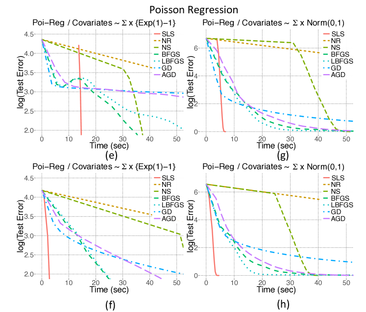
Figure 4: Additional experiments comparing the performance of SLS to that of MLE obtained with various optimization algorithms on several datasets. SLS is represented with red straight line. The details are provided in Table 3

Appendix B Additional Experiments

In this section, we provide additional experiments. The overall setting is the same as Section 9. The only difference is that we change the sampling distribution of the datasets, which are stated in the title of each plot. As in Section 9, SLS estimator outperforms its competitors by a large margin in terms of the computation time.

The results are provided in Figures 4 and 5, and Table 3.

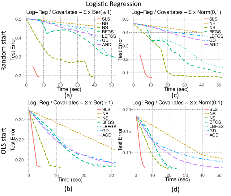
Figure 5: Additional experiments comparing the performance of SLS to that of MLE obtained with various optimization algorithms on several datasets. SLS is represented with red straight line. The details are provided in Table 3

Table 3: Details of the experiments shown in Figures 4 and 5.

Model	Logistic Regression				Poisson Regression
Dataset	${\boldsymbol{\Sigma}}\times$Ber($\pm 1$)		${\boldsymbol{\Sigma}}\times$Norm(0,1)		${\boldsymbol{\Sigma}}\times${Exp(1)-1}		${\boldsymbol{\Sigma}}\times$Norm(0,1)
Size	$n=6.0\!\times\!10^{5}$, $p\!=\!300$		$n=6.0\!\times\!10^{5}$, $p\!=\!300$		$n=6.0\!\times\!10^{5}$, $p\!=\!300$		$n=6.0\!\times\!10^{5}$, $p\!=\!300$
Initialize​​	Rnd	Ols	Rnd	Ols	Rnd	Ols	Rnd	Ols
Plot​	(a)	(b)	(c)	(d)	(e)	(f)	(g)	(h)
Method$\downarrow$​​	Time in Seconds / Number of Iterations  (to reach min test error)
Sls	6.61/3	2.97/3	9.38/5	4.25/4	14.68/4	2.99/4	6.66/10	4.13/10
Nr	222.21/6	84.08/3	186.33/6	115.76/4	218.1/6	218.9/4	364.63/9	363.4/9
Ns	40.68/10	11.57/3	53.06/9	19.52/4	39.22/6	59.61/4	51.48/10	39.8/10
Bfgs	125.83/33	35.41/9	155.3/48	24.78/8	46.61/20	48.71/12	92.84/36	74.22/38
LBfgs	142.09/38	44.41/12	444.62/143	21.79/7	96.53/39	50.56/12	296.4/111	228.1/117
Gd	409.9/134	79.45/22	1773.1/509	135.62/44	569.1/211	124.31/48	792.3/344	1041.1/366
Agd	177.3/159	43.76/12	359.56/95	53.73/18	157.9/57	63.16/16	74.74/32	62.21/32

Appendix C Auxiliary Lemmas

Lemma C.1 (Sub-exponential vector concentration).

Let $x_{1},x_{2},...,x_{n}$ be independent centered sub-exponential random vectors with $\max_{i}\|x_{i}\|_{\psi_{1}}=\kappa$. Then we have

$$\mathbb{P}\left(\left\|\frac{1}{n}\sum_{i=1}^{n}x_{i}\right\|_{2}>c\kappa\sqrt{\frac{p}{n}}\right)\leq\exp\left\{-p\right\}.$$ (C.1)

whenever $n>4c^{2}p$ for an absolute constant $c$.

Proof of Lemma C.1.

For a vector $z\in{\mathbb{R}}^{p}$, we have $\left\|z\right\|_{2}=\sup_{\left\|u\right\|_{2}=1}{\langle u,z\rangle}$ since the dual of $\ell_{2}$ norm is itself. Therefore, we write

$$\mathbb{P}\left(\left\|\frac{1}{n}\sum_{i=1}^{n}x_{i}\right\|_{2}>t\right)= \mathbb{P}\left(\sup_{\left\|u\right\|_{2}=1}\frac{1}{n}\sum_{i=1}^{n}{\langle u,x_{i}\rangle}>t\right).$$

Now, let $\mathcal{N}_{\epsilon}$ be an ${\epsilon}$-net over $\mathcal{S}^{p-1}=\{u\in{\mathbb{R}}^{p}:\ \left\|u\right\|_{2}=1\}$, and observe that

$$\max_{u\in\mathcal{N}_{\epsilon}}\ \langle u,x\rangle\geq (1-{\epsilon})\sup_{\left\|u\right\|_{2}=1}\langle u,x\rangle,$$

$$= (1-{\epsilon})\|x\|_{2},$$

with $\left|\mathcal{N}_{\epsilon}\right|\leq(1+2/{\epsilon})^{p}$. Hence, we may write

$$\mathbb{P}\left(\sup_{\left\|u\right\|_{2}=1}\frac{1}{n}\sum_{i=1}^{n}{\langle u,x_{i}\rangle}>t\right)\leq \mathbb{P}\left(\max_{u\in\mathcal{N}_{\epsilon}}\frac{1}{n}\sum_{i=1}^{n}{\langle u,x_{i}\rangle}>{t}(1-{\epsilon})\right),$$

$$\leq \left|\mathcal{N}_{\epsilon}\right|\mathbb{P}\left(\frac{1}{n}\sum_{i=1}^{n}{\langle u,x_{i}\rangle}>t(1-{\epsilon})\right).$$

For any $u\in\mathcal{S}^{p-1}$, we have $\left\|{\langle u,x_{i}\rangle}\right\|_{\psi_{1}}\leq\kappa$. Then, by the Bernstein-type inequality for sub-exponential random variables [Ver10], we have

$$\mathbb{P}\left(\frac{1}{n}\sum_{i=1}^{n}{\langle u,x_{i}\rangle}>{t}(1-{\epsilon})\right)\leq\exp\left\{-cn\min\left\{\frac{t^{2}(1-{\epsilon})^{2}}{\kappa^{2}},\frac{t(1-{\epsilon})}{\kappa}\right\}\right\},$$

for an absolute constant $c$. Therefore, the probability on the left hand side of (C.1) can be bounded by

$$\left(1+\frac{2}{{\epsilon}}\right)^{p}\exp\left\{-cn\frac{t^{2}(1-{\epsilon})^{2}}{\kappa^{2}}\right\}= \exp\left\{-cn\frac{t^{2}(1-{\epsilon})^{2}}{\kappa^{2}}+p\log\left(1+\frac{2}{{\epsilon}}\right)\right\},$$

whenever $t<\kappa/(1-{\epsilon})$. Choosing ${\epsilon}=0.5$ and for an absolute constant $c^{\prime}>3.24/c$ and letting

$$t=c^{\prime}\kappa\sqrt{\frac{p}{n}},$$

we conclude the proof. ∎

Lemma C.2.

Let $B(\tilde{\beta})$ denote the ball centered around $\tilde{\beta}$ with radius $\delta$, i.e.,

$$B(\tilde{\beta})=\left\{\beta:\big{\|}\beta-\tilde{\beta}\big{\|}_{2}\leq\delta\right\}.$$

For $i=1,...,n$, let $x_{i}\in{\mathbb{R}}^{p}$ be i.i.d. centered sub-Gaussian random vectors with norm bounded by $\kappa$ and $\mathbb{E}\left[\left\|x\right\|_{2}\right]=\tilde{\mu}\sqrt{p}$. Given a function $g:{\mathbb{R}}\to{\mathbb{R}}$ that is uniformly bounded by $b>0$, and Lipschitz continuous with $k$,

$$\mathbb{P}\left(\sup_{\beta\in B}\left|\frac{1}{n}\sum_{i=1}^{n}g(\langle x_{i},\beta\rangle)-\mathbb{E}\left[g(\langle x,\beta\rangle)\right]\right|>c(b+\kappa/\tilde{\mu})\sqrt{\frac{p}{n/\log(n)}}\right)\leq 2\exp\left\{-p\right\},$$

whenever $np>51\max\{\chi,\chi^{-1}\}$ for $\chi=(b+\kappa/\tilde{\mu})^{2}/(c\delta^{2}k^{2}\tilde{\mu}^{2})$. Above, $c$ is an absolute constant.

Proof of Lemma C.2.

Let $\mathbb{E}\left[\|x\|_{2}\right]=\mu=\tilde{\mu}\sqrt{p}$ and for ${\epsilon}>0$, $\beta\in B(\tilde{\beta})$ and $w\in{\mathbb{R}}^{p}$ define the bounding functions

$$l_{\beta}(w)= g(\langle w,\beta\rangle)-{\epsilon}{\|w\|_{2}}/{4\mu},$$

$$u_{\beta}(w)= g(\langle w,\beta\rangle)+{\epsilon}{\|w\|_{2}}/{4\mu}.$$

Let $\mathcal{N}_{\Delta}$ be a net over $B(\tilde{\beta})$ in the sense that for any $\beta_{1}\in B(\tilde{\beta})$, $\exists\beta_{2}\in\mathcal{N}_{\Delta}$ such that $\left\|\beta_{1}-\beta_{2}\right\|_{2}\leq\Delta$. We fix $\Delta_{*}=\epsilon/(4k\mu)$ and write $\forall\beta_{1}\in B$, $\exists\beta_{2}\in\mathcal{N}_{\Delta_{*}}$,

1. an upper bound of the form:

   $$g({\langle w,\beta_{1}\rangle})\leq g({\langle w,\beta_{2}\rangle})+k\left|{\langle w,\beta_{1}-\beta_{2}\rangle}\right|,$$

   $$\leq g({\langle w,\beta_{2}\rangle})+k\left\|w\right\|_{2}\Delta_{*},$$

   $$= u_{\beta_{2}}(w),$$

2. and a lower bound of the form:

   $$g({\langle w,\beta_{1}\rangle})\geq g({\langle w,\beta_{2}\rangle})-k\left|{\langle w,\beta_{1}-\beta_{2}\rangle}\right|,$$

   $$\geq g({\langle w,\beta_{2}\rangle})-k\left\|w\right\|_{2}\Delta_{*},$$

   $$= l_{\beta_{2}}(w),$$

where the second steps in the above inequalities follow from the Cauchy-Schwarz inequality. These functions are called bracketing functions in the context of empirical process theory.

Hence, we can write that $\forall\beta_{1}\in B(\tilde{\beta})$, $\exists\beta_{2}\in\mathcal{N}_{\Delta_{*}}$ such that

$$\frac{1}{n}\sum_{i=1}^{n}l_{\beta_{2}}(x_{i})-\mathbb{E}\left[l_{\beta_{2}}(x)\right]-{\epsilon}/2 \leq\frac{1}{n}\sum_{i=1}^{n}g(\langle x_{i},\beta_{1}\rangle)-\mathbb{E}\left[g(\langle x,\beta_{1}\rangle)\right],$$

$$\leq\frac{1}{n}\sum_{i=1}^{n}u_{\beta_{2}}(x_{i})-\mathbb{E}\left[u_{\beta_{2}}(x)\right]+{\epsilon}/2.$$

The above inequalities translate to the following conclusion: Whenever the following event happens,

$$\left\{\left|\frac{1}{n}\sum_{i=1}^{n}g(\langle x_{i},\beta_{1}\rangle)-\mathbb{E}\left[g(\langle x,\beta_{1}\rangle)\right]\right|>{\epsilon}\right\},$$

at least one of the following events happens

$$\left\{\frac{1}{n}\sum_{i=1}^{n}u_{\beta_{2}}(x_{i})-\mathbb{E}\left[u_{\beta_{2}}(x)\right]>{\epsilon}/2\right\}\ \ \text{or}\ \ \left\{\frac{1}{n}\sum_{i=1}^{n}l_{\beta_{2}}(x_{i})-\mathbb{E}\left[l_{\beta_{2}}(x)\right]<-{\epsilon}/2\right\}.$$

Therefore, using the union bound on the above events, we may obtain

$$\mathbb{P}\left(\sup_{\beta\in B(\tilde{\beta})}\left|\frac{1}{n}\sum_{i=1}^{n}g(\langle x_{i},\beta\rangle)-\mathbb{E}\left[g(\langle x,\beta\rangle)\right]\right|>{\epsilon}\right)$$ (C.2)

$$\leq\mathbb{P}\left(\max_{\beta\in\mathcal{N}_{\Delta_{*}}}\frac{1}{n}\sum_{i=1}^{n}u_{\beta}(x_{i})-\mathbb{E}\left[u_{\beta}(x)\right]>{\epsilon}/2\right)$$

$$\ \ +\mathbb{P}\left(\max_{\beta\in\mathcal{N}_{\Delta_{*}}}\frac{1}{n}\sum_{i=1}^{n}l_{\beta}(x_{i})-\mathbb{E}\left[l_{\beta}(x)\right]<-{\epsilon}/2\right).$$

Note that the right hand side of the above inequality has two terms both of which are of the same form. For simplicity, we bound only the first one. The bound for the second one follows from the exact same steps.

The relation between sub-Gaussian and sub-exponential norms [Ver10] allows us to write

$$\|\|x\|_{2}\|^{2}_{\psi_{2}}\leq\|\|x\|^{2}_{2}\|_{\psi_{1}}\leq \sum_{i=1}^{p}\|x_{i}^{2}\|_{\psi_{1}},$$ (C.3)

$$\leq 2\sum_{i=1}^{p}\|x_{i}\|^{2}_{\psi_{2}}\leq 2\kappa^{2}p,$$

where the second step follows from the triangle inequality. Hence, we conclude that $\|x\|_{2}-\mathbb{E}\left[\|x\|_{2}\right]$ is a centered sub-Gaussian random variable with norm upper bounded by $3\kappa\sqrt{p}$.

For ${\epsilon}<4/3$, we notice that the random variable $u_{\beta}(x)=g(\langle x,\beta\rangle)+{\epsilon}{\|x\|_{2}}/{4\mu}$ is also sub-Gaussian with norm

$$\|u_{\beta}(x)\|_{\psi_{2}} \leq b+\frac{\epsilon}{4\tilde{\mu}}3\kappa$$

$$\leq b+\kappa/\tilde{\mu},$$

and consequently, the centered random variable $u_{\beta}(x)-\mathbb{E}\left[u_{\beta}(x)\right]$ has the sub-Gaussian norm upper bounded by $2b+2\kappa/\tilde{\mu}$.

Then, by the Hoeffding-type inequality for the sub-Gaussian random variables, we obtain

$$\mathbb{P}\left(\frac{1}{n}\sum_{i=1}^{n}u_{\beta}(x_{i})-\mathbb{E}\left[u_{\beta}(x)\right]>{\epsilon}/2\right)\leq \exp\left\{-cn\frac{{\epsilon}^{2}}{(b+\kappa/\tilde{\mu})^{2}}\right\}$$

for an absolute constant $c>0$.

By the same argument above, one can obtain the same result for the function $l_{\beta}(x)$. Using Hoeffding bounds in (C.2) along with the union bound over the net, we immediately obtain

$$\mathbb{P}\left(\sup_{\beta\in B(\tilde{\beta})}\left|\frac{1}{n}\sum_{i=1}^{n}g(\langle x_{i},\beta\rangle)-\mathbb{E}\left[g(\langle x,\beta\rangle)\right]\right|>{\epsilon}\right)\leq 2\left|\mathcal{N}_{\Delta_{*}}\right|\exp\left\{-cn\frac{{\epsilon}^{2}}{(b+\kappa/\tilde{\mu})^{2}}\right\}$$

for some absolute constant $c$.

Using a standard covering argument over the net $\mathcal{N}_{\Delta_{*}}$ as given in Lemma C.3, we have

$$\left|\mathcal{N}_{\Delta_{*}}\right|\leq\left(\frac{\delta\sqrt{p}}{\Delta_{*}}\right)^{p}=\left(\frac{4\delta k\tilde{\mu}p}{{\epsilon}}\right)^{p}.$$

Combining this with the previous bound, and choosing

$${\epsilon}^{2}=\frac{p}{n}\frac{(b+\kappa/\tilde{\mu})^{2}}{2c}\log\left(\frac{32c\delta^{2}k^{2}\tilde{\mu}^{2}pn}{(b+\kappa/\tilde{\mu})^{2}}\right)$$

we get

$$2\left(\frac{4\delta k\tilde{\mu}p}{{\epsilon}}\right)^{p}\exp\left\{-cn\frac{{\epsilon}^{2}}{(b+\kappa/\tilde{\mu})^{2}}\right\}$$

$$=2\exp\left\{-\frac{p}{2}\log\log\left(\frac{32c\delta^{2}k^{2}\tilde{\mu}^{2}pn}{(b+\kappa/\tilde{\mu})^{2}}\right)\right\}$$

$$\leq 2\exp\left\{-p\right\},$$

whenever $np>51\max\{\chi,\chi^{-1}\}$ for $\chi=(b+\kappa/\tilde{\mu})^{2}/(c\delta^{2}k^{2}\tilde{\mu}^{2})$.

∎

Lemma C.3 ([EM15]).

Let $B\subset{\mathbb{R}}^{p}$ be the ball of radius $\delta$ centered around some $\beta\in{\mathbb{R}}^{p}$ and $\mathcal{N}_{\epsilon}$ be an ${\epsilon}$-net over $B$. Then,

$$\left|\mathcal{N}_{\epsilon}\right|\leq\left(\frac{\delta\sqrt{p}}{{\epsilon}}\right)^{p}.$$

Proof of Lemma C.3.

The set $B$ can be contained in a $p$-dimensional cube of size $2\delta$. Consider a grid over this cube with mesh width $2{\epsilon}/\sqrt{p}$. Then $B$ can be covered with at most $(2\delta/(2{\epsilon}/\sqrt{p}))^{p}$ many cubes of edge length $2{\epsilon}/\sqrt{p}$. If ones takes the projection of the centers of such cubes onto $B$ and considers the circumscribed balls of radius ${\epsilon}$, we may conclude that $B$ can be covered with at most

$$\left(\frac{2\delta}{2{\epsilon}/\sqrt{p}}\right)^{p}$$

many balls of radius ${\epsilon}$. ∎

Lemma C.4 (Corollary 5.50 of [Ver10]).

Let $w_{1},w_{2},...,w_{n}$ be isotropic random vectors with sub-Gaussian norm upper bounded by $\kappa$. Then for every $t>0$, with probability at least $1-2\exp\left\{-c_{1}t^{2}\right\}$, the empirical covariance $\widetilde{{\boldsymbol{\Sigma}}}$ satisfies,

$$\left\|\widetilde{{\boldsymbol{\Sigma}}}-\mathbb{I}\right\|_{2}\leq\max\{\delta,\delta^{2}\}\ \ \ \text{where}\ \ \ \delta=c_{2}\sqrt{\frac{p}{n}}+\frac{t}{\sqrt{n}}$$

where $c_{1},c_{2}$ are constants depending only on $\kappa$.

Remark 1.

For $t=\sqrt{p/c_{1}}$, we get with probability at least $1-2\exp\left\{-p\right\}$,

$$\left\|\widetilde{{\boldsymbol{\Sigma}}}-\mathbb{I}\right\|_{2}\leq C\sqrt{\frac{p}{n}}$$

where

$$C=\left\{c_{2}+\frac{1}{\sqrt{c_{1}}}\right\},$$

and $n>C^{2}p$. Here, $C$ only depends on $\kappa$.

Lemma C.5 (Corollary 5.52 of [Ver10]).

Let $x_{1},x_{2},...,x_{n}$ be random vectors with mean 0 and covariance ${\boldsymbol{\Sigma}}$ supported on a centered Euclidean ball of radius $\sqrt{R}$, i.e., $\|x_{i}\|_{2}\leq\sqrt{R}$. For ${\epsilon}\in(0,1)$ and $c>0$ an absolute constant, with probability at least $1-1/p^{2}$, the empirical covariance matrix satisfies

$$\left\|\widehat{\boldsymbol{\Sigma}}-{\boldsymbol{\Sigma}}\right\|_{2}\leq{\epsilon}\left\|{\boldsymbol{\Sigma}}\right\|_{2},$$

for $n>cR\log(p)/({\epsilon}^{2}\left\|{\boldsymbol{\Sigma}}\right\|_{2})$.

References

• [BD99] J. A. Blackard and D. J. Dean, Comparative accuracies of artificial neural networks and discriminant analysis in predicting forest cover types from cartographic variables, Comput. Electron. Agr. 24 (1999), 131–151.
• [Bis95] C. M. Bishop, Neural Networks for Pattern Recognition, Oxford University Press, 1995.
• [Bri82] D. R Brillinger, A generalized linear model with ”Gaussian” regressor variables, A Festschrift For Erich L. Lehmann, CRC Press, 1982, pp. 97–114.
• [Bro70] Charles G Broyden, The convergence of a class of double-rank minimization algorithms 2. the new algorithm, IMA Journal of Applied Mathematics 6 (1970), no. 3, 222–231.
• [BSS05] Andreas Buja, Werner Stuetzle, and Yi Shen, Loss functions for binary class probability estimation and classification: Structure and applications.
• [BSW14] Pierre Baldi, Peter Sadowski, and Daniel Whiteson, Searching for exotic particles in high-energy physics with deep learning, Nature communications 5 (2014).
• [BV04] S. Boyd and L. Vandenberghe, Convex Optimization, Cambridge University Press, 2004.
• [CGS10] L. H. Y. Chen, L. Goldstein, and Q.-M. Shao, Normal approximation by Stein’s method, Springer, 2010.
• [DLFU13] Paramveer Dhillon, Yichao Lu, Dean P Foster, and Lyle Ungar, New subsampling algorithms for fast least squares regression, Advances in Neural Information Processing Systems, 2013, pp. 360–368.
• [DMMS11] Petros Drineas, Michael W. Mahoney, S. Muthukrishnan, and Sarlòs, Faster least squares approximation, Numer. Math. 117 (2011), no. 2.
• [EBD16] Murat A Erdogdu, Mohsen Bayati, and Lee H Dicker, Scaled least squares estimator for glms in large-scale problems, Advances in Neural Information Processing Systems, 2016.
• [EM15] Murat A Erdogdu and Andrea Montanari, Convergence rates of sub-sampled newton methods, Advances in Neural Information Processing Systems, 2015, pp. 3052–3060.
• [Erd15a] Murat A Erdogdu, Newton-stein method: A second order method for glms via stein’s lemma, Advances in Neural Information Processing Systems, 2015, pp. 1216–1224.
• [Erd15b]  , Newton-stein method: An optimization method for glms via stein’s lemma, arXiv preprint arXiv:1511.08895 (2015).
• [Fis36] R. A. Fisher, The use of multiple measurements in taxonomic problems, Annals Eugenic 7 (1936), 179–188.
• [Fle70] Roger Fletcher, A new approach to variable metric algorithms, The computer journal 13 (1970), no. 3, 317–322.
• [Gol70] Donald Goldfarb, A family of variable-metric methods derived by variational means, Mathematics of computation 24 (1970), no. 109, 23–26.
• [Gol07] L. Goldstein, $l^{1}$ bounds in normal approximation, Annals Probability 35 (2007), 1888–1930.
• [GR97] L. Goldstein and G. Reinert, Stein’s method and the zero bias transformation with application to simple random sampling, Annals of Applied Probability 7 (1997), 935–952.
• [HKW99] David P Helmbold, Jyrki Kivinen, and Manfred K Warmuth, Relative loss bounds for single neurons, IEEE Transactions on Neural Networks 10 (1999), no. 6, 1291–1304.
• [HS52] M. R. Hestenes and E. Stiefel, Methods of conjugate gradients for solving linear systems, J. Res. Nat. Bur. Stand. 49 (1952), 409–436.
• [KF09] D. Koller and N. Friedman, Probabilistic Graphical Models: Principles and Techniques, MIT press, 2009.
• [LD89] K.-C. Li and N. Duan, Regression analysis under link violation, Annals of Statistics 17 (1989), 1009–1052.
• [LD09] Bing Li and Yuexiao Dong, Dimension reduction for nonelliptically distributed predictors, The Annals of Statistics (2009), 1272–1298.
• [Li91] Ker-Chau Li, Sliced inverse regression for dimension reduction, Journal of the American Statistical Association 86 (1991), no. 414, 316–327.
• [Mar10] James Martens, Deep learning via hessian-free optimization, Proceedings of the 27th International Conference on Machine Learning (ICML-10), 2010, pp. 735–742.
• [MN89] P. McCullagh and J. A. Nelder, Generalized Linear Models, 2nd ed., Chapman and Hall, 1989.
• [NB72] John A Nelder and R. Jacob Baker, Generalized linear models, Wiley Online Library, 1972.
• [Nes83] Y. Nesterov, A method of solving a convex programming problem with convergence rate $O(1/k^{2})$, Soviet Math. Dokl. 27 (1983), 372–376.
• [Nes04]  , Introductory Lectures on Convex Optimization: A Basic Course, Springer, 2004.
• [PS75] C. C. Paige and M. A. Saunders, Solution of sparse indefinite systems of linear equations, SIAM Journal of Numerical Analysis 12 (1975), 617–629.
• [PV15] Y. Plan and R. Vershynin, The generalized lasso with non-linear observations, 2015, arXiv preprint arXiv:1502.04071.
• [PW15] Mert Pilanci and Martin J Wainwright, Newton sketch: A linear-time optimization algorithm with linear-quadratic convergence, arXiv preprint arXiv:1505.02250 (2015).
• [RKM16] Farbod Roosta-Khorasani and Michael W Mahoney, Sub-sampled newton methods i: globally convergent algorithms, arXiv preprint arXiv:1601.04737 (2016).
• [RT08] V. Rokhlin and M. Tygert, A fast randomized algorithm for overdetermined linear least-squares regression, P. Natl. Acad. Sci. 105 (2008), 13212–13217.
• [RW10] Mark D Reid and Robert C Williamson, Composite binary losses, Journal of Machine Learning Research 11 (2010), no. Sep, 2387–2422.
• [Sch89] Mark J Schervish, A general method for comparing probability assessors, The Annals of Statistics (1989), 1856–1879.
• [Sha70] David F Shanno, Conditioning of quasi-newton methods for function minimization, Mathematics of computation 24 (1970), no. 111, 647–656.
• [TAH15] Christos Thrampoulidis, Ehsan Abbasi, and Babak Hassibi, Lasso with non-linear measurements is equivalent to one with linear measurements, Advances in Neural Information Processing Systems, 2015, pp. 3420–3428.
• [Ver10] R. Vershynin, Introduction to the non-asymptotic analysis of random matrices, 2010, arXiv:1011.3027.
• [WJ08] M. J. Wainwright and M. I. Jordan, Graphical models, exponential families, and variational inference, Foundations and Trends in Machine Learning 1 (2008), 1–305.