Path integrals for awkward actions

Abstract

Time derivatives of scalar fields occur quadratically in textbook actions. A simple Legendre transformation turns the lagrangian into a hamiltonian that is quadratic in the momenta. The path integral over the momenta is gaussian. Mean values of operators are euclidian path integrals of their classical counterparts with positive weight functions. Monte Carlo simulations can estimate such mean values.

This familiar framework falls apart when the time derivatives do not occur quadratically. The Legendre transformation becomes difficult or so intractable that one can’t find the hamiltonian. Even if one finds the hamiltonian, it usually is so complicated that one can’t path-integrate over the momenta and get a euclidian path integral with a positive weight function. Monte Carlo simulations don’t work when the weight function assumes negative or complex values.

This paper solves both problems. It shows how to make path integrals without knowing the hamiltonian. It also shows how to estimate complex path integrals by combining the Monte Carlo method with parallel numerical integration and a lookup table. This “Atlantic City” method lets one estimate the energy densities of theories that, unlike those with quadratic time derivatives, may have finite energy densities. It may lead to a theory of dark energy.

The approximation of multiple integrals over weight functions that assume negative or complex values is the long-standing sign problem. The Atlantic City method solves it for problems in which numerical integration leads to a positive weight function.

I Introduction

Despite the success of renormalization, infinities remain a major problem in quantum field theory. This problem grows more important as cosmological observations continue to support the existence of dark energy Ade and others (Planck Collaboration), which may be the energy density of empty space. We need to be able to compute finite energy densities. This paper advances theories of scalar fields a step closer to that goal.

The ground-state energy of a theory is the low-temperature limit of the logarithmic derivative of the partition function $Z(\beta)$ with respect to the inverse temperature $\beta$. If the action density $L$ is quadratic in the time derivatives $\dot{\phi}=\dot{\phi}_{1},\dots,\dot{\phi}_{n}$ of the fields, then a linear Legendre transformation gives a hamiltonian $H$ that is quadratic in the momenta $\pi=\pi_{1},\dots,\pi_{n}$. One can use the hamiltonian to write the partition function as a euclidian path integral in which the momentum integrals are gaussian. Integrating over the momenta, one gets the partition function as a path integral of a probability distribution in the fields. One then can use Monte Carlo methods to estimate the partition function and the mean values of various observables.

This simple framework falls apart when the time derivatives do not occur quadratically. This collapse is unfortunate because theories of scalar fields that are quadratic in the time derivatives of the fields have infinite energy densities.

An awkward action is one that is not quadratic in the time derivatives but that is simple enough for one to find its hamiltonian. One typically can’t integrate over the momentum $\pi$, and the partition function is a double path integral with a complex weight function Weinberg (1995)

$$Z(\beta)={} \int\exp\left\{\int_{0}^{\beta}\int\left[i\dot{\phi}\pi-H(\phi,\pi)\right]dt\,d^{3}x\right\}D\phi D\pi.$$ (1)

Standard Monte Carlo methods fail when the weight function assumes negative or complex values.

A very awkward action is one in which the time derivatives of the fields are related to their momenta, the fields, and their spatial derivatives by equations that are not even quartic and so have no algebraic solutions. Very awkward actions usually have no known hamiltonians. To study the ground states of this wide class of theories, we show in Sec. III how to write the partition function of such a theory as a path integral without knowledge of the hamiltonian. Our formula Cahill (2015) is a double path integral over the fields $\phi$ and over auxilliary time derivatives $\dot{\psi}$

$$\begin{split}Z(\beta)={}&\!\int\exp\bigg{\{}\int_{0}^{\beta}\!\int\Big{[}(i\dot{\phi}_{\ell}-\dot{\psi}_{\ell})\frac{\partial L(\phi,\dot{\psi})}{\partial\dot{\psi}_{\ell}}+L(\phi,\dot{\psi})\Big{]}dtd^{3}x\bigg{\}}\left|\det\!\left(\frac{\partial^{2}L(\phi,\dot{\psi})}{\partial\dot{\psi}_{k}\partial\dot{\psi}_{\ell}}\right)\right|\,D\phi D\dot{\psi}\end{split}$$ (2)

in which the $n\times n$ determinant is over the indices $k=1,\dots,n$ and $\ell=1,\dots,n$ of the fields. We give four examples of this formula, in one of which we incidentally show that the classical energy of the Nambu-Gotō string is identically zero. The path integral (2), like the one (1) for awkward actions, has a complex weight function that is not a probability distribution. Again the usual Monte Carlo methods do not work. Both path integrals are examples of what has been called the sign problem.

To estimate such complex path integrals, we introduce in Sec. IV a way that combines the Monte Carlo method with parallel numerical integration and lookup tables. In theories with awkward actions, we numerically integrate over the momenta $\pi$ in the double path integral (1). In theories with very awkward actions, we numerically integrate over the auxilliary time derivatives $\dot{\psi}$ in the double path integral (2). In both cases, we store the values of the integrals in lookup tables and then use the lookup tables to guide standard Monte Carlo estimates. We call this the Atlantic City way. It is well suited to parallel computation and may solve some versions of the sign problem. We demonstrate and test the method by applying it to a quantum-mechanical version of the scalar Born-Infeld model Born and Infeld (1934a); *Born:1934dia; *Born:1935ap considered as a theory with an awkward action in Sec. V and as a theory with a very awkward action in Sec. VI. In Sec. VII, we extend the Atlantic City way to field theory and use it to estimate the known Green’s functions of the scalar free field theory. The paper ends with a summary (Sec. VIII) and an appendix.

The paper does not discuss theories of fields with non-zero spin or higher derivatives Bender and Mannheim (2008a); *BenderMannheim2008 or those in which some fields have no time derivatives Dirac (1950); *Dirac1958; *Dirac1964.

II Review of Legendre transformations and path integrals

The lagrangian of a theory tells us about symmetries and equations of motion, but one needs a hamiltonian to determine the time evolution of states and their energies. To find the hamiltonian of a theory of scalar fields $\phi=\{\phi_{1},\dots,\phi_{n}\}$, one defines the conjugate momenta $\pi=\{\pi_{1},\dots,\pi_{n}\}$ as the derivatives of the action density

$$\pi_{j}=\frac{\partial L}{\partial\dot{\phi}_{j}},$$ (3)

and inverts these equations so as to write the time derivatives $\dot{\phi}_{j}=\dot{\phi}_{j}(\phi,\pi)$ of the fields in terms of the fields $\phi_{\ell}$ (and possibly their spatial derivatives) and their momenta $\pi_{\ell}$. The hamiltonian density then is

$$H=\sum_{j=1}^{n}\pi_{j}\dot{\phi}_{j}(\phi,\pi)-L(\phi,\dot{\phi}(\phi,\pi)).$$ (4)

When the action is quadratic in the time derivatives, Legendre’s equations (3) are linear.

Once one has a hamiltonian, one inserts complete sets of eigenstates of the fields $\phi_{j}$ and their conjugate momenta $\pi_{j}$ into the Boltzmann operator $\exp(-\beta H)=(\exp(-\beta H/n))^{n}$ and writes the partition function as the complex path integral Weinberg (1995)

$$Z(\beta)={}{\rm Tr}\,e^{-\beta H}=\int\langle\phi|e^{-\beta H}|\phi\rangle D\phi=\int\exp\left\{\int_{0}^{\beta}\int\left[i\dot{\phi}_{j}\pi_{j}-H(\phi,\pi)\right]dt\,d^{3}x\right\}D\phi D\pi.$$ (5)

If one can integrate over the momenta, then one gets Feynman’s formula Weinberg (1995); Cahill (2013a)

$$Z(\beta)={}\int\exp\left[\int_{0}^{\beta}\int{}-L_{e}(\phi,\dot{\phi})\,dt\,d^{3}x\right]D\phi$$ (6)

in which $L_{e}$ is the euclidian action density, and $D\phi$ is suitably redefined. In textbook theories, $L_{e}$ is real and positive, and the exponential $\exp[{}-L_{e}(\phi,\dot{\phi})]$ is a probability distribution well-suited to Monte Carlo methods.

This procedure is straightforward when the action is quadratic in its time derivatives, and the integrals over the momenta are gaussian. But when the equations (3) that define the momenta have square roots, the hamiltonian usually has a square root. When those equations are cubic or quartic, the Legendre transformation and the hamiltonian are complicated. When they are worse than quartic, no algebraic solution exists, and the hamiltonian typically is unknown. We show how to make path integrals for such very awkward actions in Sec. III.

III Path integrals for very awkward actions

Our solution to the problem of making a path integral without a hamiltonian is to use delta functionals to impose Legendre’s relation (3) between momenta and the fields and their derivatives. Our formula for the partition function is a double path integral over the fields $\phi$ and over auxiliary time derivatives $\dot{\psi}$

$$\begin{split}Z(\beta)={}&\!\int\exp\bigg{\{}\int_{0}^{\beta}\!\int\Big{[}(i\dot{\phi}_{\ell}-\dot{\psi}_{\ell})\frac{\partial L(\phi,\dot{\psi})}{\partial\dot{\psi}_{\ell}}+L(\phi,\dot{\psi})\Big{]}dtd^{3}x\bigg{\}}\left|\det\!\left(\frac{\partial^{2}L(\phi,\dot{\psi})}{\partial\dot{\psi}_{k}\partial\dot{\psi}_{\ell}}\right)\right|\,D\phi D\dot{\psi}\end{split}$$ (7)

in which the $n\times n$ determinant converts $D\dot{\psi}$ into $D\pi$, and the energy density

$$E(\phi,\dot{\psi})={}\dot{\psi}_{\ell}\,\frac{\partial L(\phi,\dot{\psi})}{\partial\dot{\psi}_{\ell}}-L(\phi,\dot{\psi})$$ (8)

is the hamiltonian density when the time derivatives $\dot{\psi}_{\ell}$ respect Legendre’s relation (3). If the action is time independent, then the spatial integral of $E(\phi,\dot{\psi})$ is a constant when $\dot{\psi}_{\ell}=\dot{\phi}_{\ell}(\phi,\pi)$, and the equations of motion are obeyed.

The double path integral (7) for the partition function $Z(\beta)$ is complex and ill-suited to estimation by Monte Carlo methods. We solve this problem in section IV.

To derive our formula (7), we write the path integral (5) as

$$\begin{split}Z(\beta)={}&\int\exp\left\{\int_{0}^{\beta}\int\left[i\,\dot{\phi}_{j}\pi_{j}-(\pi_{k}\dot{\psi}_{k}-L(\phi,\dot{\psi}))\right]dtd^{3}x\right\}\\ {}&\times\exp\left[i\int\left(\pi_{\ell}-\frac{\partial L}{\partial\dot{\psi}_{\ell}}\right)a_{\ell}\,d^{4}x\right]\left|\det\left(\frac{\partial^{2}L}{\partial\dot{\psi}_{k}\partial\dot{\psi}_{\ell}}\right)\right|D\phi D\pi D\dot{\psi}Da\end{split}$$ (9)

in which the integration over the $n$ auxiliary fields $a_{\ell}$ makes the second exponential a delta functional $\delta[\pi-\partial L/\partial\dot{\psi}]$ that enforces the definition (3) of the momentum $\pi_{j}$ as the derivative of the action density $L$ with respect to the time derivative $\dot{\phi}_{j}$. The jacobian is an $n\times n$ determinant that converts $D\dot{\psi}$ to $D\pi$. The integration is over all fields that are periodic with period $\beta$. Integrating first over $a$, we get

$$\begin{split}Z(\beta)={}&\int\exp\left\{\int_{0}^{\beta}\int\left[i\dot{\phi}_{j}\pi_{j}-(\pi_{k}\dot{\psi}_{k}-L(\phi,\dot{\psi}))\right]dtd^{3}x\right\}\\ {}&\times\left\{\prod_{\ell=1}^{n}\delta\left[\pi_{\ell}-\frac{\partial L}{\partial\dot{\psi}_{\ell}}\right]\right\}\left|\det\left(\frac{\partial^{2}L}{\partial\dot{\psi}_{k}\partial\dot{\psi}_{\ell}}\right)\right|D\phi D\pi D\dot{\psi}.\end{split}$$ (10)

To integrate over the auxiliary time derivatives $\dot{\psi}$, we recall the delta-function rule that if a vector $g(x)=(g_{1}(x_{1},\dots,x_{n}),\dots,g_{n}(x_{1},\dots,x_{n}))$ is zero only at $x=x^{0}$, then

$$\delta^{n}(g_{1}(x_{1},\dots,x_{n}),\dots,g_{n}(x_{1},\dots,x_{n}))\left|\det\left(\frac{\partial g_{k}(x)}{\partial x_{\ell}}\right)\right|={}\delta^{n}(x_{1}-x^{0}_{1},\dots,x_{n}-x^{0}_{n}).$$ (11)

Thus integrating the triple path integral (10) over $\dot{\psi}$, we find that the delta functional and the jacobian require the time derivatives to assume the values $\dot{\psi}_{0}(\phi,\pi)=\dot{\phi}(\phi,\pi)$ that satisfy the definition (3) of the momenta, and we get the path integral (5) over $\phi$ and $\pi$

$$\begin{split}Z(\beta)={}&\int\exp\left\{\int_{0}^{\beta}\int\left[i\dot{\phi}\pi-(\pi\dot{\psi}_{0}(\phi,\pi)-L(\phi,\dot{\psi}_{0}(\phi,\pi)))\right]dtd^{3}x\right\}D\phi D\pi\\ ={}&\int\exp\left\{\int_{0}^{\beta}\int\left[i\dot{\phi}_{j}\pi_{j}-H(\phi,\pi)\right]dt\,d^{3}x\right\}D\phi D\pi.\end{split}$$ (12)

On the other hand, if we integrate the triple path integral (10) over $\pi$, then we get our proposed formula (7)

$$\begin{split}Z(\beta)={}&\!\int\exp\left\{\int_{0}^{\beta}\!\int\left[(i\dot{\phi}_{\ell}-\dot{\psi}_{\ell})\frac{\partial L(\phi,\dot{\psi})}{\partial\dot{\psi}_{\ell}}+L(\phi,\dot{\psi})\right]dtd^{3}x\right\}\left|\det\left(\frac{\partial^{2}L(\phi,\dot{\psi})}{\partial\dot{\psi}_{k}\partial\dot{\psi}_{\ell}}\right)\right|D\phi D\dot{\psi}.\end{split}$$ (13)

This functional integral generalizes the path integral to theories of scalar fields in which the hamiltonian is unknown. A similar formula should work in theories of vector and tensor fields, apart from the issue of constraints.

Our first example is a free scalar field with action density

$$L=-\frac{1}{2}\,\partial_{\mu}\phi\,\partial^{\mu}\phi-\frac{1}{2}m^{2}\phi^{2}.$$ (14)

The determinant in our formula (13) is unity because

$$\frac{\partial^{2}L(\phi,\dot{\psi})}{\partial\dot{\psi}^{2}}=1.$$ (15)

Using the abbreviation

$$\int_{0}^{\beta}dt\!\int d^{3}x\,\equiv\int^{\beta}d^{4}x,$$ (16)

we see that the proposed path integral (13) for the free field theory (14) is

$$\begin{split}Z(\beta)={}&\int\exp\left\{\int^{\beta}\left[L(\phi,\dot{\psi})+\dot{\psi}(i\dot{\phi}-\dot{\psi})\right]d^{4}x\right\}D\phi D\dot{\psi}\\ ={}&\int\exp\left\{\int^{\beta}\left[\frac{1}{2}\dot{\psi}^{2}-\frac{1}{2}(\nabla\phi)^{2}-\frac{1}{2}m^{2}\phi^{2}+\dot{\psi}(i\dot{\phi}-\dot{\psi})\right]d^{4}x\right\}D\phi D\dot{\psi}\\ ={}&\int\exp\left\{\int^{\beta}\left[{}-\frac{1}{2}\left(\dot{\psi}-i\dot{\phi}\right)^{2}-\frac{1}{2}\dot{\phi}^{2}-\frac{1}{2}(\nabla\phi)^{2}-\frac{1}{2}m^{2}\phi^{2}\right]d^{4}x\right\}D\phi D\dot{\psi}\\ ={}&\int\exp\left\{\int^{\beta}\left[{}-\frac{1}{2}\dot{\phi}^{2}-\frac{1}{2}(\nabla\phi)^{2}-\frac{1}{2}m^{2}\phi^{2}\right]d^{4}x\right\}D\phi\\ ={}&\int\exp\left[{}-\int^{\beta}\!\!L_{e}(\phi,\dot{\phi})\,d^{4}x\right]D\phi\end{split}$$ (17)

the standard result.

Our second example is the scalar Born-Infeld theory Born and Infeld (1934a); *Born:1934dia; *Born:1935ap with action density

$$L={}M^{4}\left(1-\sqrt{1-M^{-4}\left(\dot{\phi}^{2}-(\nabla\phi)^{2}-m^{2}\phi^{2}\right)}\right)$$ (18)

and conjugate momentum

$$\pi=\frac{\partial L(\phi,\dot{\phi})}{\partial\dot{\phi}}=\frac{\dot{\phi}}{\sqrt{1-M^{-4}\left(\dot{\phi}^{2}-(\nabla\phi)^{2}-m^{2}\phi^{2}\right)}}.$$ (19)

The proposed path integral (13) is

$$\begin{split}Z(\beta)={}&\int\exp\left\{\int^{\beta}\left[(i\dot{\phi}-\dot{\psi})\frac{\partial L(\phi,\dot{\psi})}{\partial\dot{\psi}}+L(\phi,\dot{\psi})\right]d^{4}x\right\}\left|\frac{\partial^{2}L(\phi,\dot{\psi})}{\partial\dot{\psi}^{2}}\right|D\phi D\dot{\psi}\end{split}$$ (20)

in which

$$\frac{\partial L(\phi,\dot{\psi})}{\partial\dot{\psi}}=\frac{\dot{\psi}}{\sqrt{1-M^{-4}\left(\dot{\psi}^{2}-(\nabla\phi)^{2}-m^{2}\phi^{2}\right)}}$$ (21)

and

$$\frac{\partial^{2}L(\phi,\dot{\psi})}{\partial\dot{\psi}^{2}}={}\frac{1+M^{-4}\left((\nabla\phi)^{2}+m^{2}\phi^{2}\right)}{\left[1-M^{-4}\left(\dot{\psi}^{2}-(\nabla\phi)^{2}-m^{2}\phi^{2}\right)\right]^{3/2}}.$$ (22)

Substituting these formulas into (20) gives

$$\begin{split}Z(\beta)={}&\int\exp\Bigg{\{}\int^{\beta}\Bigg{[}\frac{(i\dot{\phi}-\dot{\psi})\dot{\psi}}{\sqrt{1-M^{-4}\left(\dot{\psi}^{2}-(\nabla\phi)^{2}-m^{2}\phi^{2}\right)}}\\ {}&{}+M^{4}\left(1-\sqrt{1-M^{-4}\left(\dot{\psi}^{2}-(\nabla\phi)^{2}-m^{2}\phi^{2}\right)}\right)\Bigg{]}d^{4}x\Bigg{\}}\\ {}&\times\frac{1+M^{-4}\left((\nabla\phi)^{2}+m^{2}\phi^{2}\right)}{\left[1-M^{-4}\left(\dot{\psi}^{2}-(\nabla\phi)^{2}-m^{2}\phi^{2}\right)\right]^{3/2}}\,D\phi D\dot{\psi}.\end{split}$$ (23)

We can set

$$\pi={}\frac{\partial L(\phi,\dot{\psi})}{\partial\dot{\psi}}=\frac{\dot{\psi}}{\sqrt{1-M^{-4}\left(\dot{\psi}^{2}-(\nabla\phi)^{2}-m^{2}\phi^{2}\right)}}$$ (24)

and so absorb the jacobian in

$$d\pi={}\frac{\partial\pi}{\partial\dot{\psi}}\,d\dot{\psi}=\frac{\partial^{2}L(\phi,\dot{\psi})}{\partial\dot{\psi}^{2}}\,d\dot{\psi}={}\frac{1+M^{-4}\left((\nabla\phi)^{2}+m^{2}\phi^{2}\right)}{\left[1-M^{-4}\left(\dot{\psi}^{2}-(\nabla\phi)^{2}-m^{2}\phi^{2}\right)\right]^{3/2}}\,d\dot{\psi}.$$ (25)

The partition function (23) then is

$$\begin{split}Z(\beta)={}&\int\exp\Bigg{[}\int^{\beta}(i\dot{\phi}-\dot{\psi})\pi+M^{4}\left(1-\sqrt{1-\left(\dot{\psi}^{2}-(\nabla\phi)^{2}-m^{2}\phi^{2}\right)/M^{4}}\right)d^{4}x\Bigg{]}D\phi D\pi\end{split}$$ (26)

where now $\dot{\psi}(\phi,\pi)$ is the function of $\phi$ and $\pi$ defined by (24).

The action of this theory is awkward, but not very awkward. We can solve Legendre’s equation (24) for the time derivative $\dot{\phi}$

$$\dot{\phi}=\frac{\pi}{\sqrt{1+M^{-4}\,\pi^{2}}}\sqrt{1+M^{-4}\left((\nabla\phi)^{2}+m^{2}\phi^{2}\right)}$$ (27)

and find as the hamiltonian density

$$\begin{split}H(\phi,\pi)={}&\pi\dot{\phi}-L(\phi,\dot{\phi})\\ ={}&\frac{\pi^{2}\sqrt{1+M^{-4}\left((\nabla\phi)^{2}+m^{2}\phi^{2}\right)}}{\sqrt{1+M^{-4}\,\pi^{2}}}-M^{4}\\ {}&+M^{4}\sqrt{1-M^{-4}\left(\frac{\pi^{2}\left(1+M^{-4}\left((\nabla\phi)^{2}+m^{2}\phi^{2}\right)\right)}{1+M^{-4}\,\pi^{2}}-(\nabla\phi)^{2}-m^{2}\phi^{2}\right)}\\ ={}&\frac{\pi^{2}\sqrt{M^{4}+(\nabla\phi)^{2}+m^{2}\phi^{2}}}{\sqrt{M^{4}+\pi^{2}}}+M^{4}\frac{\sqrt{M^{4}+(\nabla\phi)^{2}+m^{2}\phi^{2}}}{\sqrt{M^{4}+\pi^{2}}}-M^{4}\\ ={}&\sqrt{\left(M^{4}+\pi^{2}\right)\left(M^{4}+(\nabla\phi)^{2}+m^{2}\phi^{2}\right)}-M^{4}.\end{split}$$ (28)

Thus for this theory, the double path integral (1) is

$$\begin{split}Z(\beta)={}&\int\exp\left\{\int^{\beta}\left[i\dot{\phi}\pi{}-\sqrt{\left(M^{4}+\pi^{2}\right)\left(M^{4}+(\nabla\phi)^{2}+m^{2}\phi^{2}\right)}+M^{4}\right]d^{4}x\right\}D\phi D\pi.\end{split}$$ (29)

Our third example is the theory defined by the action density

$$L=M^{4}\exp(L_{0}/M^{4})$$ (30)

in which $L_{0}$ is the action density (14) of the free field. The derivatives of $L$ are

$$\frac{\partial L}{\partial\dot{\psi}}=M^{-4}\dot{\psi}\,L\quad\mbox{and}\quad\frac{\partial^{2}L}{\partial\dot{\psi}^{2}}=M^{-4}(1+M^{-4}\dot{\psi}^{2})\,L.$$ (31)

So the proposed path integral is

$$\begin{split}Z(\beta)={}&\int\exp\left\{\int^{\beta}\left[L(\phi,\dot{\psi})+\frac{\partial L(\phi,\dot{\psi})}{\partial\dot{\psi}}(i\dot{\phi}-\dot{\psi})\right]d^{4}x\right\}\left|\frac{\partial^{2}L(\phi,\dot{\psi})}{\partial\dot{\psi}^{2}}\right|D\phi D\dot{\psi}\\ ={}&\int\exp\left\{\int^{\beta}\left[1+\frac{\dot{\psi}(i\dot{\phi}-\dot{\psi})}{M^{4}}\right]L(\phi,\dot{\psi})\,d^{4}x\right\}M^{-4}(1+M^{-4}\dot{\psi}^{2})\,L\,D\phi D\dot{\psi}.\end{split}$$ (32)

Our fourth example is the Nambu-Gotō action density

$$L={}-T_{0}\,\sqrt{\left(\dot{X}\cdot X^{\prime}\right)^{2}-\left(\dot{X}\right)^{2}\left(X^{\prime}\right)^{2}}$$ (33)

in which the tau or time derivatives of the coordinate fields $X^{\mu}$ do not occur quadratically Cahill (a). The momenta are

$$\mathcal{P}^{\tau}_{\mu}=\frac{\partial L}{\partial\dot{X}^{\mu}}={}-T_{0}\,\frac{(\dot{X}\cdot X^{\prime})X^{\prime}_{\mu}-(X^{\prime})^{2}\dot{X}_{\mu}}{\sqrt{\left(\dot{X}\cdot X^{\prime}\right)^{2}-\left(\dot{X}\right)^{2}\left(X^{\prime}\right)^{2}}}$$ (34)

and the second derivatives of the Lagrange density are

$$\begin{split}\frac{\partial^{2}L}{\partial\dot{X}^{\mu}\partial\dot{X}^{\nu}}={}&T_{0}\,\left[\frac{\eta_{\mu\nu}X^{\prime 2}-X^{\prime}_{\mu}X^{\prime}_{\nu}}{\sqrt{\left(\dot{X}\cdot X^{\prime}\right)^{2}-\left(\dot{X}\right)^{2}\left(X^{\prime}\right)^{2}}}\right.\\ {}&\left.-\frac{\left((\dot{X}\cdot X^{\prime})X^{\prime}_{\mu}-(X^{\prime})^{2}\dot{X}_{\mu}\right)\left((\dot{X}\cdot X^{\prime})X^{\prime}_{\nu}-(X^{\prime})^{2}\dot{X}_{\nu}\right)}{\left[\left(\dot{X}\cdot X^{\prime}\right)^{2}-\left(\dot{X}\right)^{2}\left(X^{\prime}\right)^{2}\right]^{3/2}}\right].\end{split}$$ (35)

The proposed partition function (13) for the Nambu-Gotō action is then

$$\begin{split}Z(\beta)={}&\!\!\int\!\exp\!\left\{\int^{\beta}\left[(i\dot{X}^{\mu}-\dot{Y}^{\mu})\frac{\partial L(X,\dot{Y})}{\partial\dot{Y}^{\mu}}+L(X,\dot{Y})\right]d\sigma d\tau\right\}\left|\det\!\left[\frac{\partial^{2}L(X,\dot{Y})}{\partial\dot{Y}^{\mu}\partial\dot{Y}^{\nu}}\right]\right|DXD\dot{Y}\end{split}$$ (36)

in which the formulas (34) and (35) (with $\dot{X}^{\mu}\to\dot{Y}^{\mu}$) are to be substituted for the first and second derivatives of the action density $L$ with respect to the tau derivatives $\dot{Y}^{\mu}$. But because the action density $L$ is a homogeneous function of degree 1 of the time (and space) derivatives of the fields $X^{\mu}$, its energy density vanishes independently of the equations of motion

$$E={}\dot{X}^{\mu}\frac{\partial L}{\dot{X}^{\mu}}-L=0$$ (37)

by Euler’s theorem. Thus the partition function (36) is simply

$$\begin{split}Z(\beta)={}&\!\!\int\!\exp\!\left[\int^{\beta}i\dot{X}^{\mu}\frac{\partial L(X,\dot{Y})}{\partial\dot{Y}^{\mu}}d\sigma d\tau\right]\left|\det\!\left[\frac{\partial^{2}L(X,\dot{Y})}{\partial\dot{Y}^{\mu}\partial\dot{Y}^{\nu}}\right]\right|DXD\dot{Y}.\end{split}$$ (38)

But since we know that the hamiltonian (37) vanishes, we can use the simpler formula (5) and get for the partition function the badly divergent expression

$$\begin{split}Z(\beta)={}&\!\!\int\!\exp\!\left[\int^{\beta}i\dot{X}^{\mu}\mathcal{P}^{\tau}_{\mu}\,d\sigma d\tau\right]DXD\mathcal{P}.\end{split}$$ (39)

IV The Atlantic City method

Monte Carlos let us estimate the mean values of observables weighted by probability distributions Cahill (b). They fail when the weight function assumes negative or complex values. This failure is one aspect of the sign problem. The double-ratio trick (99–100) outlined in the appendix A is unreliable.

These problems are not hopeless however. For although the weight functions of the double path integrals (1) and (2) are complex, the integrals of these complex weight functions over the momenta $\pi$ or over the auxiliary time derivatives $\dot{\psi}$ are real and positive. They are the probability distribution that determines the partition function and the mean values of observables.

If one can’t do these integrals analytically, one can do them numerically. These numerical integrations are well suited to parallel computation. In the Atlantic City method, one numerically integrates in parallel over the momenta $\pi$ or over the auxiliary time derivatives $\dot{\psi}$ in the double path integrals (1 or 2) and stores the values of these integrals in a lookup table. One then uses the Monte Carlo method guided by the stored integrals to estimate the mean values of observables.

Our main goal is to study the ground states of field theories, but for simplicity in this paper we will explain and test the Atlantic City method in the context of quantum mechanics.

If the action is awkward, but not very awkward, then we can find the hamiltonian $H(q,p)$ but can’t integrate analytically over the momentum $p$. Then the partition function $Z(\beta)$ is

$$\begin{split}Z(\beta)={}&{\rm Tr}\,e^{-\beta H}=\int\exp\left\{\int_{0}^{\beta}\left[i\dot{q}p-H(q,p)\right]dt\right\}DpDq.\end{split}$$ (40)

We use the approximation

$$\begin{split}\langle q_{\ell+1}|e^{-aH(q,p)}|q_{\ell}\rangle\approx{}&\int dp\,\langle q_{\ell+1}|p\rangle\langle p|e^{-aH(q_{\ell},p)}|q_{\ell}\rangle\\ ={}&\int_{-\infty}^{\infty}\frac{dp}{\sqrt{2\pi}}\,\exp\left[i(q_{\ell+1}-q_{\ell})p\,-a\,H(q_{\ell},p)\right]\end{split}$$ (41)

to estimate the partition function as the multiple integral

$$\begin{split}Z(\beta)={}&\prod_{j=1}^{n}\int\frac{dp_{j}dq_{j}}{2\pi}\exp\left[i(q_{j+1}-q_{j})p_{j}-aH(q_{j},p_{j})\right]\end{split}$$ (42)

in which $n=\beta/a$, and the paths are periodic $q_{n+1}=q_{1}$.

The path integral

$$P[q,\beta]={}\int\exp\left\{\int_{0}^{\beta}\left[i\dot{q}p-H(q,p)\right]dt\right\}Dp$$ (43)

is an unnormalized functional probability distribution that assigns a number $P[q,\beta]$ to every path $q(t)$. It is the limit as $n\to\infty$ and $a=\beta/n\to 0$ of the multiple integral

$$P_{n}[q,\beta]={}\prod_{j=1}^{n}\int\frac{dp_{j}}{\sqrt{2\pi}}\exp\left[i(q_{j+1}-q_{j})p_{j}-aH(q_{j},p_{j})\right].$$ (44)

If the hamiltonian is even in the momentum, then this probability distribution is real

$$P_{n}[q,\beta]={}\prod_{j=1}^{n}\int\frac{dp_{j}}{\sqrt{2\pi}}\cos[(q_{j+1}-q_{j})p_{j}]e^{-aH(q_{j},p_{j})}.$$ (45)

The partition function $Z(\beta)$ is

$$\begin{split}Z(\beta)={}&\int P[q,\beta]\,Dq={}\int\prod_{j=1}^{n}\frac{dq_{j}}{\sqrt{2\pi}}\,P_{n}[q,\beta].\end{split}$$ (46)

The mean value of the energy at inverse temperature $\beta$ is

$$\begin{split}\langle H\rangle_{\beta}={}\frac{{\rm Tr}\,H\,e^{-\beta H}}{{\rm Tr}\,e^{-\beta H}}={}&-\frac{1}{Z(\beta)}\frac{dZ(\beta)}{d\beta}=-\frac{1}{Z(\beta)}\int\prod_{j=1}^{n}\frac{dq_{j}}{\sqrt{2\pi}}\,\frac{dP_{n}[q,\beta]}{d\beta}.\end{split}$$ (47)

The derivative of the probability distribution with respect to $\beta=n\,a$ is

$$\begin{split}{}-\frac{dP_{n}[q,\beta]}{d\beta}={}&\frac{1}{n}\sum_{k=1}^{n}\int\prod_{j=1}^{n}\frac{dp_{j}}{\sqrt{2\pi}}\,H(q_{k},p_{k})\,e^{i(q_{j+1}-q_{j})p_{j}-aH(q_{j},p_{j})}.\end{split}$$ (48)

So the mean value of the hamiltonian at inverse temperature $\beta$ is

$$\begin{split}\langle H\rangle_{\beta}={}&\frac{1}{n}\sum_{k=1}^{n}\int\prod_{j=1}^{n}dq_{j}\,dp_{j}\,\,H(q_{k},p_{k})\,e^{i(q_{j+1}-q_{j})p_{j}-aH(q_{j},p_{j})}\\ {}&\left/\int\prod_{j=1}^{n}dq_{j}\,dp_{j}\,e^{i(q_{j+1}-q_{j})p_{j}-aH(q_{j},p_{j})}\right..\end{split}$$ (49)

In the Atlantic City method, one does the $p$ integrations numerically, setting

$$\begin{split}A(q_{\ell+1},q_{\ell})=\int_{-\infty}^{\infty}\frac{dp}{\sqrt{2\pi}}\,\exp\left[i(q_{\ell+1}-q_{\ell})p\,-a\,H(q_{\ell},p)\right]\end{split}$$ (50)

and

$$C(q_{\ell+1},q_{\ell})={}\int_{-\infty}^{\infty}\frac{dp}{\sqrt{2\pi}}\,H(q_{\ell},p)\,\exp\left[i(q_{\ell+1}-q_{\ell})p\,-a\,H(q_{\ell},p)\right].$$ (51)

If one uses $N$ values of $q_{\ell}$, then one does these $2N^{2}$ numerical integrals. One may do them in parallel.

In most problems of interest, the hamiltonian is an even function of the momentum, $H(q,-p)=H(q,p)$, and the integrals (50 & 51) are real

$$\begin{split}A(q_{\ell+1},q_{\ell})={}&\sqrt{\frac{2}{\pi}}\int_{0}^{\infty}dp\,\cos\left[(q_{\ell+1}-q_{\ell})\,p\right]\,e^{-a\,H(q_{\ell},p)}\\ C(q_{\ell+1},q_{\ell})={}&\sqrt{\frac{2}{\pi}}\int_{0}^{\infty}dp\,H(q_{\ell},p)\,\cos\left[(q_{\ell+1}-q_{\ell})\,p\right]\,e^{-a\,H(q_{\ell},p)}.\end{split}$$ (52)

One’s tables need run only over $q_{\ell+1}\geq q_{\ell}$. We have found it convenient to use the variables $dq_{\ell}=|q_{\ell+1}-q_{\ell}|$ and $q_{\ell}$ and to adjust the resolution of the tables according to the variation of the integrals $A(dq_{\ell},q_{\ell})$ and $C(dq_{\ell},q_{\ell})$.

In terms of these numerical integrals, the mean value of the hamiltonian is

$$\begin{split}\langle H\rangle_{\beta}={}&\frac{1}{n}\sum_{k=1}^{n}\int dq_{k}\prod_{j=1,\,j\neq k}^{n}\!dq_{j}\,C(q_{k+1},q_{k})\,A(q_{j+1},q_{j})\left/\int\prod_{j=1}^{n}dq_{j}\,A(q_{j+1},q_{j})\right.\end{split}$$ (53)

which we may write as

$$\begin{split}\langle H\rangle_{\beta}={}&\frac{1}{n}\sum_{k=1}^{n}\int\prod_{j=1}^{n}\!dq_{j}\,\frac{C(q_{k+1},q_{k})}{A(q_{k+1},q_{k})}\,A(q_{j+1},q_{j})\left/\int\prod_{j=1}^{n}dq_{j}\,A(q_{j+1},q_{j})\right..\end{split}$$ (54)

We do a Monte Carlo over the probability distribution

$$P(q)={}\left.\prod_{j=1}^{n}A(q_{j+1},q_{j})\right/\int\prod_{j=1}^{n}dq_{j}\,A(q_{j+1},q_{j})$$ (55)

and measure the ratio

$$\langle H\rangle_{\beta}={}\left\langle\frac{1}{n}\sum_{k=1}^{n}\frac{C(q_{k+1},q_{k})}{A(q_{k+1},q_{k})}\right\rangle=\int\frac{1}{n}\sum_{k=1}^{n}\frac{C(q_{k+1},q_{k})}{A(q_{k+1},q_{k})}\,P(q)\,Dq.$$ (56)

When the hamiltonian is a monotonically increasing, even function of the momentum, the integration (52) for $A(q_{\ell+1},q_{\ell})$ is positive over every interval

$$\frac{2\pi n}{\Delta q_{\ell}}\,\leq\,{}p\,\leq{}\frac{2\pi(n+1)}{\Delta q_{\ell}}$$ (57)

for $n=0,1,2\dots$ where $\Delta q_{\ell}=q_{\ell+1}-q_{\ell}$. The reason is that when $H(q_{\ell},p)$ increases with $p$, the positive integral from $p=2\pi n/\Delta q_{\ell}$ to $p=2\pi(n+{\textstyle{\frac{1}{2}}})/\Delta q_{\ell}$ weighted by $\exp(-aH(q_{\ell},p))$ with $p$ in that interval exceeds the negative integral from $p=2\pi(n+{\textstyle{\frac{1}{2}}})/\Delta q_{\ell}$ to $p=2\pi(n+1)/\Delta q_{\ell}$ weighted by $\exp(-aH(q_{\ell},p))$ with $p$ in this second interval.

Thus as long as the hamiltonian is a monotonically increasing, even function of the momentum, the product $A(q_{j+1},q^{\prime}_{j})\,A(q^{\prime}_{j},q_{j-1})$ will be an unnormalized probability distribution in the variable $q^{\prime}_{j}$. It is a simple matter to have one’s Monte Carlo code report the minimum value of the integral $A(q_{\ell+1},q_{\ell})$ (52) and to check that it is positive.

To take a Metropolis step, we pick a new $q^{\prime}_{j}$ and look up the value of the (unnormalized) probability distribution

$$P(q^{\prime}_{j})={}A(q_{j+1},q^{\prime}_{j})\,A(q^{\prime}_{j},q_{j-1}).$$ (58)

Usually, the random points $q_{j+1}$, $q^{\prime}_{j}$, and $q_{j-1}$ are not be among the $q_{j}$’s in our tables, so our computers use a bilinear interpolation to approximate $A(q_{j+1},q^{\prime}_{j})$ and $A(q^{\prime}_{j},q_{j-1})$.

If $P(q^{\prime}_{j})\geq P(q_{j})$, then we accept the new $q^{\prime}_{j}$. If $P(q^{\prime}_{j})<P(q_{j})$, then we accept the new $q^{\prime}_{j}$ with conditional probability

$$P(q_{j}\to q^{\prime}_{j})=P(q_{j}^{\prime})/P(q_{j})$$ (59)

and otherwise reject it.

V Application of the Atlantic City method to the Born-Infeld oscillator

In this section we demonstrate and test our Atlantic City model on a theory with an awkward action, the quantum-mechanical version of the scalar Born-Infeld model (18–29). The lagrangian of this model is

$$L={}Mc^{2}-Mc^{2}\left[1-\frac{m}{Mc^{2}}\left(\dot{q}^{2}-\omega^{2}q^{2}\right)\right]^{1/2}.$$ (60)

The momentum is

$$p={}\frac{m\dot{q}}{\sqrt{1-m\left(\dot{q}^{2}-\omega^{2}q^{2}\right)/(Mc^{2})}},$$ (61)

and the velocity is

$$\dot{q}={}\frac{p}{m}\frac{\sqrt{1+m\omega^{2}q^{2}/Mc^{2}}}{\sqrt{1+p^{2}/(mMc^{2})}}.$$ (62)

The hamiltonian of the Born-Infeld oscillator is

$$H={}\sqrt{\left(p^{2}/m+Mc^{2}\right)\,\,\left(Mc^{2}+m\omega^{2}q^{2}\right)}-Mc^{2}.$$ (63)

In terms of the hamiltonian $H_{0}=p^{2}/2m+m\omega^{2}q^{2}/2$ of the harmonic oscillator, the hamiltonian $H$ of the Born-Infeld oscillator in the limit $M/m\gg 1$ is

$$\begin{split}H={}&H_{0}-\frac{1}{8Mc^{2}}\left(\frac{p^{2}}{2m}-\frac{m\omega^{2}q^{2}}{2}\right)^{2}\left(1-\frac{H_{0}}{Mc^{2}}\right)+\dots\end{split}$$ (64)

and

$$H={}\sqrt{Mc^{2}m\omega^{2}q^{2}}\Big{[}1+\frac{p^{2}}{2mMc^{2}}-\frac{p^{4}}{8(mMc^{2})^{2}}\Big{]}\Big{[}1+\frac{Mc^{2}}{2m\omega^{2}q^{2}}-\frac{(Mc^{2})^{2}}{32(m\omega^{2}q^{2})^{2}}\Big{]}+\dots$$ (65)

for $M/m\ll 1$.

With $\hbar=c=1$ and $\beta=n\,a$, the partition function is

$$\begin{split}Z(\beta)={}&{\rm Tr}\,e^{-\beta H}=\int\exp\left\{\int_{0}^{\beta}\left[i\dot{q}p-H(q,p)\right]dt\right\}DpDq\\ \approx{}&\prod_{j=1}^{n}\int\frac{dp_{j}dq_{j}}{2\pi}\exp\left[i(q_{j+1}-q_{j})p_{j}-aH(q_{j},p_{j})\right]\\ \approx{}&\prod_{j=1}^{n}\int\frac{dp_{j}dq_{j}}{2\pi}\exp\left[i(q_{j+1}-q_{j})p_{j}-a\left(\sqrt{\left(p^{2}_{j}/m+M\right)\left(M+m\omega^{2}q^{2}_{j}\right)}-M\right)\right].\end{split}$$ (66)

In the limit $M=0$, the hamiltonian (63) is $H_{M=0}={}|\omega\,p\,q|$, which is so simple that we can integrate over the momentum and write the partition function as an ordinary path integral

$$\begin{split}Z(\beta)\approx{}&\prod_{j=1}^{n}\int\frac{dp_{j}dq_{j}}{2\pi}\exp\left[i(q_{j+1}-q_{j})p_{j}-a|\omega\,p_{j}\,q_{j}|\right]\\ ={}&\prod_{j=1}^{n}\int\frac{dq_{j}}{\pi}\frac{a\,|\omega\,q_{j}|}{a^{2}\,\omega^{2}q_{j}^{2}+(q_{j+1}-q_{j})^{2}}.\end{split}$$ (67)

The naive formula for the partition function is to replace $t$ by $-i\beta$ in the path integral for the amplitude

$$\langle q(t)|e^{-itH}|q(0)\rangle={}\int e^{i\int Ldt}\,Dq.$$ (68)

If we applied this rule to the action density (60) in the limit $M\to 0$ keeping $mM=1$, then we’d get for the partition function

$$Z(\beta)_{\mbox{\footnotesize{naive}}}\approx{}\prod_{j=1}^{n}\int\frac{dq_{j}}{2\pi}\,e^{-\sqrt{(q_{j+1}-q_{j})^{2}+a^{2}\omega^{2}q_{j}^{2}}}$$ (69)

which is very different from the correct formula (67).

In terms of the variables to $q^{\prime}=q\sqrt{m}$ and $p^{\prime}=p/\sqrt{m}$, which satisfy the commutation relation $[q^{\prime},p^{\prime}]=i$, the Born-Infeld hamiltonian (63) is

$$H={}\sqrt{\left(p^{\prime 2}+M\right)\,\,\left(M+\omega^{2}q^{\prime 2}\right)}-M,$$ (70)

which shows that the energy levels are independent of the mass parameter $m$. To simplify our notation and expose the actual dependence of these energies, we change variables again to $p^{\prime}=\sqrt{M}p^{\prime\prime}$ and $q^{\prime}=\sqrt{M}q^{\prime\prime}/\omega$. After we drop all the primes, we have

$$H={}M\left[\sqrt{\left(p^{2}+1\right)\,\,\left(q^{2}+1\right)}-1\right],$$ (71)

and

$$\begin{split}Z(\beta)\approx{}&\prod_{j=1}^{n}\int\frac{Mdp_{j}dq_{j}}{2\pi\omega}\exp\left\{\left[i\frac{M}{\omega}(q_{j+1}-q_{j})p_{j}-aM\left(\sqrt{\left(p^{2}_{j}+1\right)\left(q^{2}_{j}+1\right)}-1\right)\right]\right\}.\end{split}$$ (72)

The mean value of the hamiltonian at inverse temperature $\beta=na$ is

$$\begin{split}\langle H\rangle_{\beta}={}&-\frac{{\rm Tr}\,H\,e^{-\beta H}}{{\rm Tr}\,e^{-\beta H}}={}-\frac{1}{Z(\beta)}\frac{dZ(\beta)}{d\beta}={}-\frac{1}{nZ(\beta)}\frac{dZ(\beta)}{da}.\end{split}$$ (73)

The energy $\langle H\rangle_{\beta}$ is a function of the ratio $M/\omega$ and is proportional to $M$

$$\begin{split}\langle H\rangle_{\beta}={}&\prod_{j=1}^{n}\int dp_{j}dq_{j}\left[\frac{M}{n}\sum_{\ell=0}^{n}\left(\sqrt{\left(p^{2}_{j}+1\right)\left(q^{2}_{j}+1\right)}-1\right)\right]\\ {}&\times\exp\left[i\frac{M}{\omega}(q_{j+1}-q_{j})p_{j}-aM\left(\sqrt{\left(p^{2}_{j}+1\right)\left(q^{2}_{j}+1\right)}-1\right)\right]\\ {}&\left/\prod_{j=1}^{n}\int\!dp_{j}dq_{j}\exp\left[i\frac{M}{\omega}(q_{j+1}-q_{j})p_{j}-aM\left(\sqrt{\left(p^{2}_{j}+1\right)\left(q^{2}_{j}+1\right)}-1\right)\right]\right..\end{split}$$ (74)

The ground-state energy is the limit of the ratio as $\beta\to\infty$ and $a\to 0$.

We wrote Fortran 90 codes to compute in parallel the momentum integrals

$$\begin{split}A(q_{\ell+1},q_{\ell})={}&\int_{0}^{\infty}\!dp\cos\left[\frac{M}{\omega}(q_{\ell+1}-q_{\ell})p\right]\exp\left[-aM\left(\sqrt{\left(p^{2}+1\right)\left(q^{2}_{\ell}+1\right)}-1\right)\right]\end{split}$$ (75)

and

$$\begin{split}C(q_{\ell+1},q_{\ell})={}&M\int_{0}^{\infty}\!dp\left(\sqrt{\left(p^{2}+1\right)\left(q^{2}_{\ell}+1\right)}-1\right)\\ {}&\times\cos\left[\frac{M}{\omega}(q_{\ell+1}-q_{\ell})p\right]\exp\left[-aM\left(\sqrt{\left(p^{2}+1\right)\left(q^{2}_{\ell}+1\right)}-1\right)\right]\end{split}$$ (76)

for suitably large sets of values of $q_{\ell}$ and $q_{\ell+1}$ and stored them in lookup tables. We then used the lookup tables in standard Monte Carlos with a Metropolis step (58–59) to estimate the mean value of the hamiltonian at inverse temperature $\beta$

$$\langle H\rangle_{\beta}={}\left\langle\frac{1}{n}\sum_{k=1}^{n}\frac{C(q_{k+1},q_{k})}{A(q_{k+1},q_{k})}\right\rangle=\int\frac{1}{n}\sum_{k=1}^{n}\frac{C(q_{k+1},q_{k})}{A(q_{k+1},q_{k})}\,P_{n}[q,\beta]\,Dq$$ (77)

in which the unnormalized probability distribution is

$$P_{n}(q,\beta)={}\prod_{\ell=1}^{n}A(q_{\ell+1},q_{\ell})$$ (78)

and $q_{n+1}\equiv q_{1}$.

The Monte Carlo codes run fast; all the work is in the lookup tables. We made lookup tables for $0.1\leq Mc^{2}/(\hbar\omega)\leq 10$, $a\omega=0.1$, and $\beta=10^{3}/M$. We plotted our Atlantic City (75–77) estimates of the ground-state energy of the Born-Infeld oscillator as blue dots in Fig. 1 and listed them in Table 1. The integrals (75 & 76) have the exponential term $\exp[{}-aM\sqrt{(p^{2}+1)(q^{2}_{\ell}+1)}]$ and so converge faster at big $M$ for fixed $a$ and $\omega$. The statistical errors are smaller than the dots.

To test these results, we used Matlab to compute the exact eigenvalues of the Born-Infeld oscillator. In terms of the harmonic-oscillator variables $a={}\sqrt{m\omega/2}\left[q+ip/(m\omega)\right]$ and $a^{\dagger}={}\sqrt{m\omega/2}\left[q-ip/(m\omega)\right]$, the operators $q$ and $p$ are $q=\left(a^{\dagger}+a\right)/\sqrt{2m\omega}$ and $p=i\sqrt{m\omega/2}\left(a^{\dagger}-a\right)$, and so the hamiltonian (63) is

$$H={}\sqrt{Mc^{2}-\frac{\omega}{2}\left(a^{\dagger}-a\right)^{2}}\sqrt{Mc^{2}+\frac{\omega}{2}\left(a^{\dagger}+a\right)^{2}}-Mc^{2}$$ (79)

in which the mass $m$ does not appear. We made a matrix $a$ as diag(sqrt([1:Nmax]),1) with Nmax = 1000 and $a^{\dagger}$ as its transpose. The Matlab command eig(sqrtm(H)) then gave the exact energy eigenvalues, which generated the red curves in the figures and the exact results in the tables.

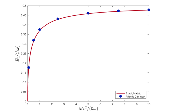
Figure 1: Our Atlantic City estimates (75–77, blue dots) of the ground-state energies $E_{0}/(\hbar\omega)$ of the Born-Infeld oscillator are plotted along with the exact values (Matlab, red curve) for $0.1\leq Mc^{2}/(\hbar\omega)\leq 10$, $a\omega=0.1$, and $\beta=10^{3}/M$.

Table 1: Exact (Matlab) and Atlantic City results (75–77) for the ground-state energy $E_{0}/(\hbar\omega)$ of the Born-Infeld hamiltonian (63) for $0.1\leq Mc^{2}/(\hbar\omega)\leq 10$.

$Mc^{2}/(\hbar\omega)$	$E_{0}/(\hbar\omega)$ exact	$E_{0}/(\hbar\omega)$ Atlantic City
0.1	0.1881	0.1759
0.5	0.3155	0.3191
1.0	0.3702	0.3746
2.5	0.4288	0.4308
5.0	0.4587	0.4603
7.5	0.4708	0.4723
10.0	0.4774	0.4781

VI The Atlantic City model applied to a very awkward action

In this section, we test our Atlantic City method by using it to find the ground-state energy of the Born-Infeld oscillator considered as a theory with a very awkward action. That is, we pretend that we don’t know the Born-Infeld hamiltonian (63) and use our Atlantic City method to evaluate the complex path integral (2) for its partition function.

Instead of the partition function (74), we have the partition function

$$\begin{split}Z(\beta)={}&\int\exp\left\{\int^{\beta}\left[(i\dot{q}-\dot{s})\frac{\partial L(q,\dot{s})}{\partial\dot{s}}+L(q,\dot{s})\right]dt\right\}\left|\frac{\partial^{2}L(q,\dot{s})}{\partial\dot{s}^{2}}\right|DqD\dot{s}\\ ={}&\int\exp\left\{\int^{\beta}\left[\frac{mi\dot{q}\dot{s}-m\omega^{2}q^{2}-M}{\sqrt{1-m\left(\dot{s}^{2}-\omega^{2}q^{2}\right)/M}}+M\right]\,dt\right\}\\ {}&\times\,\frac{m+m^{2}\omega^{2}q^{2}/M}{\left[1-m\left(\dot{s}^{2}-\omega^{2}q^{2}\right)/M\right]^{3/2}}\,DqD\dot{s}.\end{split}$$ (80)

Sending $q_{j}\to\sqrt{M/m}\,q_{j}/\omega$ and $\dot{s}_{j}\to\sqrt{M/m}\,\dot{s}_{j}$, we can write $Z(\beta)$ as

$$\begin{split}Z(\beta)={}&\int\exp\left\{\int^{\beta}\left[\frac{i(M/\omega)\dot{q}\dot{s}-Mq^{2}-M}{\sqrt{1+q^{2}-\dot{s}^{2}}}+M\right]\,dt\right\}\frac{1+q^{2}}{\left[1+q^{2}-\dot{s}^{2}\right]^{3/2}}\frac{M}{\omega}DqD\dot{s}.\end{split}$$ (81)

Setting $dt=a$ and sending $a\to a/M$, we approximate this path integral on an $n\times n$ lattice of spacing $a=\beta/n$ as the multiple integral

$$\begin{split}Z(\beta)={}&\prod_{j=1}^{n}\int\frac{Md\dot{s}_{j}dq_{j}}{2\pi\omega}\exp\left[i\frac{M}{\omega}\left(\frac{\left(q_{j+1}-q_{j}\right)\dot{s}_{j}}{\sqrt{1+q^{2}_{j}-\dot{s}^{2}_{j}}}\right)-aM\left(\frac{q^{2}_{j}+1}{\sqrt{1+q^{2}_{j}-\dot{s}^{2}_{j}}}-1\right)\right]\\ {}&\quad\times\,\frac{1+q^{2}_{j}}{\left[1+q^{2}_{j}-\dot{s}^{2}_{j}\right]^{3/2}}\end{split}$$ (82)

in which the lower limits are $q_{j}=\dot{s}_{j}=0$ and the upper limits are $q_{j}\to\infty$ and $\dot{s}_{j}\leq\sqrt{q^{2}_{j}+1}$.

Apart from the phase factor, the integrand is even in $\dot{s}$. We numerically compute the integrals

$$\begin{split}A(q_{j+1},q_{j})={}&\int_{0}^{\sqrt{q^{2}_{j}+1}}d\dot{s}\,\cos\left[\frac{M}{\omega}\left(\frac{\left(q_{j+1}-q_{j}\right)\dot{s}_{j}}{\sqrt{1+q^{2}_{j}-\dot{s}^{2}_{j}}}\right)\right]\exp\left[-aM\left(\frac{q^{2}_{j}+1}{\sqrt{1+q^{2}_{j}-\dot{s}^{2}_{j}}}-1\right)\right]\\ {}&\quad\times\,\frac{1+q^{2}_{j}}{\left[1+q^{2}_{j}-\dot{s}^{2}_{j}\right]^{3/2}}\end{split}$$ (83)

and

$$\begin{split}C(q_{j+1},q_{j})={}&M\int_{0}^{\sqrt{q^{2}_{j}+1}}d\dot{s}\,\left[\frac{q^{2}_{j}+1}{\sqrt{1+q^{2}_{j}-\dot{s}^{2}_{j}}}-1\right]\cos\left[\frac{M}{\omega}\left(\frac{\left(q_{j+1}-q_{j}\right)\dot{s}_{j}}{\sqrt{1+q^{2}_{j}-\dot{s}^{2}_{j}}}\right)\right]\\ {}&\times\exp\left[-aM\left(\frac{q^{2}_{j}+1}{\sqrt{1+q^{2}_{j}-\dot{s}^{2}_{j}}}-1\right)\right]\frac{1+q^{2}_{j}}{\left[1+q^{2}_{j}-\dot{s}^{2}_{j}\right]^{3/2}}.\end{split}$$ (84)

We do these integrals in parallel and store their values in a lookup table. We then use the lookup table and the Monte Carlo method to estimate the mean value

$$\langle H\rangle_{\beta}={}\left\langle\frac{1}{n}\sum_{k=1}^{n}\frac{C(q_{k+1},q_{k})}{A(q_{k+1},q_{k})}\right\rangle.$$ (85)

We plotted our results for $0.1\leq Mc^{2}/(\hbar\omega)\leq 10$, $a\omega=0.1$, and $\beta=10^{3}/M$ as green dots in Fig. 2 and listed them in Table 2. For comparable amounts of computation, these results are not quite as accurate as those of Table 1. The reason is that the argument of the cosine in the formulas (83 & 84) for $A(q_{j+1},q_{j})$ and $C(q_{j+1},q_{j})$ diverges as $\dot{s}^{2}\to q_{j}^{2}+1$. The integrals converge, but one needs more points at small $M$ for fixed $a$ and $\omega$.

Figure 2: Our Atlantic City estimates (83–85, blue-green dots) of the ground-state energies of the Born-Infeld oscillator are plotted along with the exact values (red curve) for $0.1\leq Mc^{2}/(\hbar\omega)\leq 10$, $a\omega=0.1$, and $\beta=10^{3}/M$.

Table 2: Exact (Matlab) and Atlantic City results (83–85) for the ground-state energies $E_{0}/(\hbar\omega)$ of the Born-Infeld oscillator (63) for $0.3\leq Mc^{2}/(\hbar\omega)\leq 8.75$.

$M/(\hbar\omega)$	$E_{0}/(\hbar\omega)$ exact	$E_{0}/(\hbar\omega)$ Atlantic City
0.3	0.2731	0.2884
0.75	0.3482	0.3599
1.75	0.4084	0.4145
3.75	0.4478	0.4502
6.25	0.4658	0.4678
8.75	0.4746	0.4766

VII Transition to field theory

In this section, we sketch how the Atlantic City method will work in field theory. Suppose the action is awkward, but not very, so that we have a hamiltonian

$$H={}H(\pi^{2},(\nabla\phi)^{2},\phi^{2}).$$ (86)

The form $\nabla\phi^{2}\equiv(\nabla\phi)^{2}$ follows from rotational invariance. The path integral for the partition function is

$$\begin{split}Z(\beta)={}&\int\exp\left\{\int^{\beta}\left[i\dot{\phi}\pi{}-H(\pi^{2},\nabla\phi^{2},\phi^{2})\right]d^{4}x\right\}D\phi D\pi.\end{split}$$ (87)

We derive this path integral from integrals of products of matrix elements like

$$\langle\phi(t+a)|\pi\rangle\langle\pi|e^{-aH}|\phi(t)\rangle,$$ (88)

and approximate it on a $n^{4}$ lattice with spacing $a$ and $\beta=na$ as

$$\begin{split}Z(\beta)\approx{}&\prod_{i,j,k,\ell=1}^{n}\int d\phi_{i,j,k,\ell}d\pi_{i,j,k,\ell}\exp\left[a^{3}i(\phi_{i,j,k,\ell+1}-\phi_{i,j,k,\ell})\pi_{i,j,k,\ell}\right.\\ {}&\left.-a^{4}H(\pi^{2}_{i,j,k,\ell},\nabla\phi^{2}_{i,j,k,\ell},\phi^{2}_{i,j,k,\ell})\right]\end{split}$$ (89)

in which the squared gradients are

$$\begin{split}(\nabla\phi)^{2}_{i,j,k,\ell}={}&\frac{(\phi_{i+1,j,k,\ell}-\phi_{i,j,k,\ell})^{2}}{a^{2}}+\frac{(\phi_{i,j+1,k,\ell}-\phi_{i,j,k,\ell})^{2}}{a^{2}}+\frac{(\phi_{i,j,k+1,\ell}-\phi_{i,j,k,\ell})^{2}}{a^{2}}.\end{split}$$ (90)

The lookup tables are three dimensional with entries

$$A(\phi_{+},\phi,\nabla\phi^{2})={}\int d\pi\,\cos[a^{3}(\phi_{+}-\phi)\pi]e^{-a^{4}H(\pi^{2},\nabla\phi^{2},\phi^{2})}$$ (91)

and if one seeks to compute the mean value of the energy density

$$C(\phi_{+},\phi,\nabla\phi^{2})={}\int d\pi\,H(\pi^{2},\nabla\phi^{2},\phi^{2})\cos[a^{3}(\phi_{+}-\phi)\pi]e^{-a^{4}H(\pi^{2},\nabla\phi^{2},\phi^{2})}.$$ (92)

We have tested the Atlantic City way by using it to estimate the euclidian Green’s functions

$$G(x,y)={}\langle 0|\mathcal{T}\left[\phi(x)\phi(y)\right]|0\rangle$$ (93)

of the free field theory (14). Using parallel computing, we made three-dimensional lookup tables of the values of $A(\phi_{+},\phi,\nabla\phi^{2})$ for $m=1$ and lattice spacings $a=1,1/2,1/4,...,1/32,$ and 0.01. We then used the standard Monte Carlo method to estimate the path integrals

$$G(x,y)={}\frac{\int\phi(x)\,\phi(y)\,A(\phi_{+},\phi,\nabla\phi^{2})\,D\phi}{\int A(\phi_{+},\phi,\nabla\phi^{2})\,D\phi}$$ (94)

on lattices as big as $80^{4}$. Our Atlantic City estimates are listed in Table 3 and plotted in Fig. 3.

Table 3: Atlantic City way estimate of the free-field Green’s function for $m=1$

$a$	$G(a)$	$G(2a)$	$G(3a)$	$G(4a)$
1.0	0.01853	0.003051	0.0005872	0.0001307
0.5	0.09947	0.02177	0.006156	0.002135
0.25	0.4462	0.1122	0.03877	0.01709
0.125	1.8643	0.4976	0.1878	0.0919
0.0625	7.6632	2.0909	0.8185	0.4185
0.03125	30.7463	8.4501	3.3537	1.7486
0.01	296.3381	81.6334	32.5551	17.0888

On an infinite lattice of spacing $a$, the exact euclidian Green’s function for $y$ at the origin and $x=(na,0,0,0)$ is Rothe (1997)

$$G(na)={}G_{\mbox{{\scriptsize lat}}}(na)={}\frac{1}{a^{2}}\int_{-\pi}^{\pi}\frac{e^{ip_{1}n}}{\left[a^{2}m^{2}+\sum_{i}4\sin^{2}(p_{i}/2)\right]}\frac{d^{4}p}{(2\pi)^{4}}.$$ (95)

We used Mathematica to numerically integrate this expression and got the values listed in Table 4. Fig. 3 shows that the agreement with our Atlantic City estimates is excellent.

Table 4: Exact infinite-lattice free-field Green’s function for $m=1$:

$a$	$G(a)$	$G(2a)$	$G(3a)$	$G(4a)$
1.0	0.0180008	0.00296172	0.000571368	0.000127571
0.5	0.0997255	0.0218474	0.00618522	0.00215997
0.25	0.450334	0.113275	0.0391267	0.0172243
0.125	1.87841	0.500742	0.189039	0.0924796
0.0625	7.61685	2.07525	0.811638	0.414713
0.03125	30.59684	8.399072	3.327155	1.728039
0.01	299.265	82.3963	32.8142	17.1637

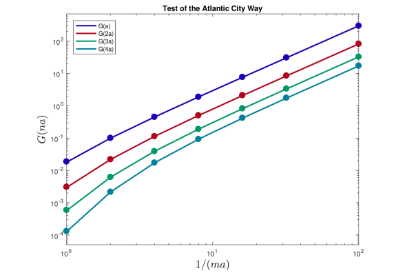
Figure 3: The exact infinite-lattice euclidian Green’s functions $G(na,0)$ (solid) for $n=1$ (blue), 2 (red), 3 (green), and 4 (blue green) and our Atlantic City estimates done on an $80^{4}$ lattice (dots).

VIII Summary

We divide the actions of theories of scalar fields into three classes—graceful, awkward, and very awkward. An action is graceful if it is quadratic in the time derivatives of the fields, which then are linearly related to the momenta, the fields, and their spatial derivatives. Its partition function is a path integral over the fields with a positive weight function. An action is awkward if it is not quadratic in the time derivatives of the fields but is simple enough for one to find its hamiltonian. One typically can’t integrate over the momenta, and the partition function is a path integral over the fields and their momenta with a complex weight function. An action is very awkward action if the equations for the time derivatives are worse than quartic, and one can’t find its hamiltonian.

We have shown how to write the partition function as a euclidian path integral when one doesn’t know the hamiltonian. We also have shown how to estimate euclidian path integrals that have weight functions that assume negative or complex values. One integrates numerically over the momenta if the action is awkward or over auxiliary time derivatives if it is very awkward. The numerical integrations are ideally suited to parallel computation. One stores the values of the integrals in lookup tables and uses them to guide standard Monte Carlos. We demonstrated and tested this Atlantic City method on the Born-Infeld oscillator by treating its action both as awkward and as very awkward. We sketched how to extend this method to field theory and tested it by computing the known euclidian Green’s functions of the free field theory.

Theories with graceful actions have infinite energy densities. The Atlantic City method lets one estimate the energy density of theories with awkward or very awkward actions, some of which may have finite or less than quartically divergent energy densities Boettcher and Bender (1990); *Cahill2013NA; *PhysRevD.88.125014NA. The Atlantic City method also provides a way to estimate the acceleration of the scale factor $a(t)$ which in terms of the energy-momentum tensor $T_{ij}$ and its trace is

$$\frac{\ddot{a}(t)}{a(t)}={}-\frac{8\pi G}{3}\left(T_{00}+\frac{T}{2}\right)$$ (96)

in theories with awkward or very awkward actions. So the Atlantic City way of estimating path integrals may lead to a theory of dark energy.

The approximation of multiple integrals with weight functions that assume negative or complex values is a long-standing problem in applied mathematics, called the sign problem. The Atlantic City method solves it for problems in which numerical integration leads to a positive weight function.

In the course of this paper, we incidentally showed that the classical hamiltonian of the Nambu-Gotō string vanishes identically and that the folk theorem linking path integrals in real and imaginary time can fail when the action is awkward or very awkward.

*

Appendix A Ratios of complex Monte Carlos are unreliable

The mean value of an observable $A[\phi]$ at inverse temperature $\beta$ is

$$\begin{split}\langle A[\phi]\rangle={}&\frac{{\rm Tr}\,A[\phi]e^{-\beta H}}{{\rm Tr}\,e^{-\beta H}}\\ ={}&\int A[\phi]\exp\left[\int\left(i\,\dot{\phi}_{j}-\dot{\psi}_{j}\right)\frac{\partial L}{\partial\dot{\psi}_{j}}+L(\phi,\dot{\psi})\,d^{4}x\right]{\left|\det\left(\frac{\partial^{2}L}{\partial\dot{\psi}_{k}\partial\dot{\psi}_{\ell}}\right)\right|}D\phi D\dot{\psi}\\ {}&\left/\int\exp\left[\int\left(i\,\dot{\phi}_{j}-\dot{\psi}_{j}\right)\frac{\partial L}{\partial\dot{\psi}_{j}}+L(\phi,\dot{\psi})\,d^{4}x\right]{\left|\det\left(\frac{\partial^{2}L}{\partial\dot{\psi}_{k}\partial\dot{\psi}_{\ell}}\right)\right|}D\phi D\dot{\psi}\right..\end{split}$$ (97)

The complex action

$$S={}\int\left(i\,\dot{\phi}_{j}-\dot{\psi}_{j}\right)\frac{\partial L}{\partial\dot{\psi}_{j}}+L(\phi,\dot{\psi})\,d^{4}x$$ (98)

oscillates and does not give us a probability distribution unless we can integrate over $D\dot{\psi}$. One can write the mean value (97) as a ratio of mean values

$$\begin{split}\langle A[\phi]\rangle={}&\left\langle A[\phi]\exp\left[\int i\,\dot{\phi}_{j}\,\frac{\partial L}{\partial\dot{\psi}_{j}}\,d^{4}x\right]\right\rangle\left/\left\langle\exp\left[\int i\,\dot{\phi}_{j}\,\frac{\partial L}{\partial\dot{\psi}_{j}}\,d^{4}x\right]\right\rangle\right.\\ ={}&\int A[\phi]\exp\left[\int i\,\dot{\phi}_{j}\,\frac{\partial L}{\partial\dot{\psi}_{j}}\,d^{4}x\right]P(\phi,\dot{\psi})D\phi D\dot{\psi}\\ {}&\quad\left/\int\exp\left[\int i\,\dot{\phi}_{j}\,\frac{\partial L}{\partial\dot{\psi}_{j}}\,d^{4}x\right]P(\phi,\dot{\psi})\,D\phi D\dot{\psi}\right.\end{split}$$ (99)

in which the functional $P(\phi,\dot{\psi})$ is a normalized probability distribution

$$\begin{split}P(\phi,\dot{\psi})={}&\exp\left[\int\left(L(\phi,\dot{\psi})-\dot{\psi}_{j}\,\frac{\partial L}{\partial\dot{\psi}_{j}}\right)d^{4}x\right]\left|\det\left(\frac{\partial^{2}L}{\partial\dot{\psi}_{k}\partial\dot{\psi}_{\ell}}\right)\right|\\ {}&\left/\int\exp\left[\int\left(L(\phi,\dot{\psi})-\dot{\psi}_{j}\,\frac{\partial L}{\partial\dot{\psi}_{j}}\right)d^{4}x\right]\left|\det\left(\frac{\partial^{2}L}{\partial\dot{\psi}_{k}\partial\dot{\psi}_{\ell}}\right)\right|\,D\phi D\dot{\psi}\right..\end{split}$$ (100)

Although in principle one can use the Monte Carlo method Cahill (2013d) to estimate the numerator $N$ and the denominator $D$ of the ratio (99), both $N$ and $D$ are the mean values of complex oscillating functionals. In many cases of interest, both $N$ and $D$ are smaller than the measurement errors $\delta N$ and $\delta D$ in computations of reasonable lengths. The error in the observable $A[\phi]$ is

$$\delta\langle A[\phi]\rangle={}\delta\frac{N}{D}=\frac{\delta N}{D}-\frac{N}{D^{2}}\delta D=\frac{\delta N}{D}-\langle A[\phi]\rangle\frac{\delta D}{D},$$ (101)

and both $N$ and $D$ often are zero in the limit in which $\beta\to\infty$.

For instance, suppose we apply the technique (99–100) to the computation of the ground-state energy $\langle H\rangle=N/D$ of the harmonic oscillator in which the numerator is

$$N={} \int\left(\frac{p^{2}}{2m}+\frac{1}{2}m\omega^{2}q^{2}\right)\exp\left[\int\left(i\dot{q}p-\frac{p^{2}}{2m}-\frac{1}{2}m\omega^{2}q^{2}\right)dt\right]DpDq$$

$$\left/\int\exp\left[\int\left(-\frac{p^{2}}{2m}-\frac{1}{2}m\omega^{2}q^{2}\right)dt\right]DpDq\right.,$$ (102)

the denominator $D$ is

$$D={} \int\exp\left[\int\left(i\dot{q}p-\frac{p^{2}}{2m}-\frac{1}{2}m\omega^{2}q^{2}\right)dt\right]DpDq$$

$$\left/\int\exp\left[\int\left(-\frac{p^{2}}{2m}-\frac{1}{2}m\omega^{2}q^{2}\right)dt\right]DpDq\right.,$$ (103)

and the measure $DpDq$ is

$$DpDq=\prod_{j=1}^{n}\frac{1}{2\pi}dp_{j}dq_{j}.$$ (104)

In the continuum limit ($n\rightarrow\infty$, $dt\rightarrow 0$, with $\beta=n\>dt$ fixed), the numerator $\mathcal{N}$ of the denominator $D\equiv\mathcal{N}/\mathcal{D}$ of the ratio $N/D$ is the partition function

$$\mathcal{N}={} Z(\beta)={\rm Tr}\,e^{-\beta H}$$

$$={} \int\exp\left[\int\left(i\dot{q}p-\frac{p^{2}}{2m}-\frac{1}{2}m\omega^{2}q^{2}\right)dt\right]DpDq$$

$$={} \frac{1}{2\sinh(\beta\omega/2)},$$ (105)

and the denominator is

$$\mathcal{D}={} \int\exp\left[\int\left(-\frac{p^{2}}{2m}-\frac{1}{2}m\omega^{2}q^{2}\right)dt\right]DpDq$$

$$={} \prod_{j=1}^{n}\int\frac{dp_{j}dq_{j}}{2\pi}\exp\left[\sum_{j=1}^{n}\left(-\frac{p^{2}_{j}}{2m}-\frac{1}{2}m\omega^{2}q^{2}_{j}\right)\frac{\beta}{n}\right]$$

$$={} \left(\frac{1}{2\pi}\right)^{n}\left(\frac{2\pi mn}{\beta}\right)^{n/2}\prod_{j=1}^{n}\int dq_{j}\exp\left[\sum_{j=1}^{n}\left(-\frac{1}{2}m\omega^{2}q^{2}_{j}\right)\frac{\beta}{n}\right]$$

$$={} \left(\frac{1}{2\pi}\right)^{n}\left(\frac{2\pi mn}{\beta}\right)^{n/2}\left(\frac{2\pi n}{m\omega^{2}\beta}\right)^{n/2}=\left(\frac{n}{\beta\omega}\right)^{n}.$$ (106)

This denominator goes to infinity as $n\to\infty$ and $\beta/n\to 0$ for any $\beta\neq 0$. So the denominator $D$ vanishes

$$D=\frac{1}{2\sinh(\beta\omega/2)\,\mathcal{D}}=0.$$ (107)

The numerator also vanishes, so the ratio $\langle H\rangle=N/D$ is hard to estimate, being $0/0$.

Thus the double-ratio trick (99–100) is not in general reliable.

References

• Ade and others (Planck Collaboration) P. Ade and others (Planck Collaboration), Astron. Astrophys. 566, A54 (2014)  (2013).
• Weinberg (1995) S. Weinberg, The Quantum Theory of Fields, Vol. I (Cambridge University Press, 1995) Chap. 9.
• Cahill (2015) K. Cahill, “Path integrals for actions that are not quadratic in their time derivatives,”  (2015), arXiv:1501.00473 [hep-th] .
• Born and Infeld (1934a) M. Born and L. Infeld, Proc. Roy. Soc. Lond. A144, 425 (1934a).
• Born and Infeld (1934b) M. Born and L. Infeld, Proc. Roy. Soc. Lond. A147, 522 (1934b).
• Born and Infeld (1935) M. Born and L. Infeld, Proc. Roy. Soc. Lond. A150, 141 (1935).
• Bender and Mannheim (2008a) C. M. Bender and P. D. Mannheim, Phys. Rev. Letters 100, 110402 (2008a).
• Bender and Mannheim (2008b) C. M. Bender and P. D. Mannheim, J. Phys. A 41, 304018 (2008b).
• Dirac (1950) P. A. M. Dirac, Can. J. Math. 2, 129 (1950).
• Dirac (1958) P. A. M. Dirac, Proc. Roy. Soc. London, ser. A 246, 326 (1958).
• Dirac (1964) P. A. M. Dirac, Lectures on Quantum Mechanics (Yeshiva University and Dover Publications, 1964).
• Cahill (2013a) K. Cahill, “Physical Mathematics,”  (Cambridge University Press, 2013) Chap. 16.
• Cahill (a) K. Cahill, ibid, Chap. 19.
• Cahill (b) K. Cahill, ibid, Chap. 14.
• Rothe (1997) H. J. Rothe, Lattice Gauge Theories: An Introduction, 2nd ed. (World Scientific, 1997) Chap. 3.
• Boettcher and Bender (1990) S. Boettcher and C. Bender, J. Math. Phys. 31(11), 2579 (1990).
• Cahill (2013b) K. Cahill, Phys. Rev. D 87, 065024 (2013b).
• Cahill (2013c) K. Cahill, Phys. Rev. D 88, 125014 (2013c).
• Cahill (2013d) K. Cahill, “Physical Mathematics,”  (Cambridge University Press, 2013) Chap. 14.