Testable Baryogenesis in Seesaw Models
NuFact 2016

Abstract

We revisit the production of baryon asymmetries in the minimal type I seesaw model with heavy Majorana singlets in the GeV range. We include “washout” effects from scattering processes with gauge bosons, higgs decays and inverse decays, besides the dominant top scatterings. We show that in the minimal model with two singlets, and for an inverted light neutrino ordering, future measurements from SHiP and neutrinoless double beta decay could in principle provide sufficient information to predict the matter-antimatter asymmetry in the universe. [1]

1 Introduction

The origin of the observed baryon asymmetry in the Universe is one of the unresolved fundamental questions. To dynamically generate the this asymmetry, three Sakharov conditions need to be fulfilled: processes that violate baryon number, processes that violate both C and CP, and the out-of equilibrium processes should be present. In the popular models of baryogenesis through leptogenesis, all three conditions are satisfied in the decay of a heavy particle, usually above TeV scale. However, in the so-called low scale seesaw model, where the masses of sterile neutrinos are below the electroweak scale, it is possible to generate the asymmetry in the lepton sector via the oscillations of the sterile states, as firstly proposed in [2]. Generated asymmetry is stored in the sterile sector at least until the time of the electroweak phase transition when the sphaleron processes that violate the baryon number become inefficient. For the asymmetry not to be washed-out sterile neutrinos should not reach thermal equilibrium. This reflects in the sterile neutrinos couplings and masses, and put them to be in the $\mathcal{O}$(GeV) scale. Note that this is exactly the mass range future experiments as SHiP [3], DUNE [4] and FCC [5] will be sensitive to, which makes this model potentially testable.

In this work we focus in two different questions: what are constraints on the parameter space of the model assyming that the described mechanism generetes all the observed baryon asymmetry, and, can we predict the baryon asymmetry if the sterile neutrinos are measured in SHiP or FCC together with the $\delta_{CP}$ phase in DUNE and the neutrinoless double beta decay effective mass $m_{\beta\beta}$.

2 Formalism

The evolution of the sterile (anti)neutrino and the lepton asymmetry in the form of chemical potential is well described by the density matrix formalism proposed by Raffelt and Sigl [7]. The previous analysis [9, 8] usually assumed the production rate of the sterile neutrinos to be dominant by the top quark scattering and the Pauli blocking terms in the kinetic equations are usually neglected. Here we derive the set of kinetic equations that beside the top quark interactions include $2\leftrightarrow 2$ scatterings at tree level with gauge bosons, as well as $1\leftrightarrow 2$ scatterings including the resummation of scatterings mediated by soft gauge bosons. Those effects were derived in [6] for the case of vanishing leptonic potential and we re-evaluated them including the chemical potential up to the linear order. We also kept Fermi-Dirac or Bose-Einstein statistic throughout and include the spectators effects.

The evolution of sterile (anti)neutrino $r_{N/\bar{N}}\equiv\rho_{N/\bar{N}}/\rho_{F}$ and the chemical potentials defined as $n_{B/3-L_{\alpha}}={T^{3}\over 6}\mu_{B/3-L_{\alpha}}$, are:

$$xH_{u}{dr_{N}\over dx} = -i[\langle H\rangle,r_{N}]-{\langle\gamma^{(0)}_{N}\rangle\over 2}\{Y^{\dagger}Y,r_{N}-1\}+\langle\gamma_{N}^{(1)}\rangle Y^{\dagger}\mu Y-{\langle\gamma_{N}^{(2)}\rangle\over 2}\big{\{}Y^{\dagger}\mu Y,r_{N}\big{\}},$$

$$xH_{u}{dr_{\bar{N}}\over dx} = -i[\langle H^{*}\rangle,r_{\bar{N}}]-{\langle\gamma^{(0)}_{N}\rangle\over 2}\{Y^{T}Y^{*},r_{\bar{N}}-1\}-\langle\gamma_{N}^{(1)}\rangle Y^{T}\mu Y^{*}+{\langle\gamma_{N}^{(2)}\rangle\over 2}\big{\{}Y^{T}\mu Y^{*},r_{\bar{N}}\big{\}},$$

$$xH_{u}{d{\mu}_{B/3-L_{\alpha}}\over dx} = {\int_{k}\rho_{F}\over\int_{k}\rho^{\prime}_{F}}\Bigg{\{}{\langle\gamma_{N}^{(0)}\rangle\over 2}(Yr_{N}Y^{\dagger}-Y^{*}r_{\bar{N}}Y^{T})_{\alpha\alpha}+\mu_{\alpha}\Bigg{(}{\langle\gamma_{N}^{(2)}\rangle\over 2}(Yr_{N}Y^{\dagger}+Y^{*}r_{\bar{N}}Y^{T})_{\alpha\alpha}$$

$$- \langle\gamma_{N}^{(1)}\rangle{\rm Tr}[YY^{\dagger}I_{\alpha}]\Bigg{)}\bigg{\}},$$

$$\mu_{\alpha} = -\sum_{\beta}C_{\alpha\beta}\mu_{B/3-L_{\beta}},$$ (1)

where $\gamma_{N}$ are momentum averaged interaction rates, $Y$ is the Yukawa matrix and $\rho_{F}$ is the Fermi-Dirac equilibrium distribution.

The baryon asymmetry is expressed in terms of $\mu_{B/3-L_{\alpha}}$ as

$$Y_{B}\simeq 1.3\times 10^{-3}\sum_{\alpha}\mu_{B/3-L_{\alpha}}.$$ (2)

The current value given by the Planck collaboration is,

$$Y_{B}^{\rm exp}\simeq 8.65(8)\times 10^{-11}.$$ (3)

The numerical solution of kinetic equations is very challenging due to the fast oscillating terms and the analytic approximations are usually made. Even though they are useful for understanding the general behavior of the solutions, they can not be applied to all the parameter space. To preform the numerical scan over all the parameter space we used MultiNest and the solution of the equations is done numerically using the public available code SQuIDS [10].

3 Results

We use a Gaussian likelihood consistent with the Planck measurement 3 and perform a Bayesian analysis of the model parameters. The results are summarized in Table 1, where we have considered flat priors in all the Casas-Ibarra parameters except the masses where we assume a flat prior in $\log_{10}\left({M_{1}\over{\rm GeV}}\right)$, within the range $M_{1}\in[0.1{\rm GeV},10^{2}{\rm GeV}]$, and two possibilities: Blue contours, with a flat prior in $\log_{10}\left({M_{2}\over GeV}\right)$ in the same range; and red contours, with a flat prior in $\log_{10}\left({|M_{2}-M_{1}|\over{\rm GeV}}\right)$ in the range $[10^{-8}{\rm GeV},10^{2}{\rm GeV}]$. The second option force the Bayesian sampling to explore the high degeneracy of the mass parameters.

NO	Prior	$M_{1}({\rm GeV})$	$\Delta M_{12}({\rm GeV})$	$|U_{e4}|^{2}$	$|U_{\mu 4}|^{2}$	$|U_{\tau 4}|^{2}$	$m_{\beta\beta}({\rm eV})$
IH	M	$-0.55^{+0.16}_{-0.38}$	$-2.23^{+0.22}_{-0.19}$	$-7.2^{+0.9}_{-0.4}$	$-8.5^{+1.0}_{-0.6}$	$-8.5^{+0.8}_{-0.7}$	$-0.84\pm 0.55$
	$\Delta$M	$0.23^{+0.68}_{-0.82}$	$-2.36^{+0.71}_{-0.51}$	$-9.2^{+1.7}_{-1.4}$	$-10.1^{+1.5}_{-1.2}$	$-9.9^{+1.4}_{-1.2}$	$-1.48^{+0.15}_{-0.28}$
NH	M	$-0.39^{+0.31}_{-0.42}$	$-3.1\pm 0.4$	$-8.9^{+0.8}_{-0.7}$	$-7.4\pm 0.7$	$-7.3^{+0.7}_{-0.5}$	$-2.66\pm 0.20$
	$\Delta$M	$0.8^{+0.82}_{-0.66}$	$-2.76\pm 0.62$	$-11.2^{1.4}_{-1.6}$	$-9.9^{+1.3}_{-1.8}$	$-10.0^{+1.3}_{-1.6}$	$-2.62\pm 0.14$

Table 1: Result for the ranges for the measured value eq.3

In Fig.1 we give the posterior probabilities of the mass differences versus the sum of the mixing matrix elements over the flavor, the electron mixing and the neutrinoless double beta decay effective mass. Note that the blue region, that represent the less fine-tuned solutions, can contribute significantly to the $m_{\beta\beta}$ and also give the higher mixings.

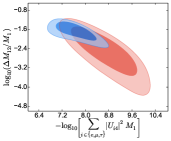
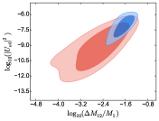
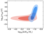
Figure 1: The mass degeneracy versus the sum of the mixing, the electron mixing and $m_{\beta\beta}$.

The mixings of the sterile state with all three neutrino flavors are given in Fig 2, where the shaded region represents the parameter space excluded from the direct searches experiment. Note that the blue region is inside the sensitivity region of the proposed SHiP experiment.

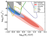
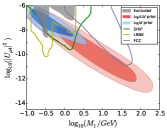
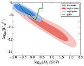
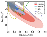
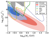
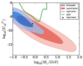
Figure 2: Contours for the active sterile matrix elements overlapped with the expected sensitivity of the proposed SHiP experiment. The plots are for electron, muon, and tau from left to right and normal and inverted mass ordering top and bottom respectively.

Next we assumed a putative measurement in SHiP, that we fix to the values denoted by the star in the Fig 2.

The correlation of the baryon asymmetry and $m_{\beta\beta}$ is presented on Fig 3, where optimistic errors of 0.1% and 1% error in the masses and mixings are considered, as well as a putative measurement of the $\delta_{CP}$ phase.

Figure 3: Baryon asymmetry as a function of the $m_{\beta\beta}$ if a putative measure of SHiP is assumed (red region), and if we assume additional measurement of the $\delta_{CP}$ phase (blue region).

The last and more detailed results about the implications of a SHiP signal in the leptonic CP-violation can be found in the paper[11].

4 Conclusion

• We have studied the production of the matter-antimatter asymmetry in low-scale ${\mathcal{O}}({\rm GeV})$ seesaw models.

• Our analysis include the washout processes from gauge interactions and Higgs decays and inverse decays, quantum statistics in the computation of all rates, as well as spectator processes. This together with a more efficient numerical treatment of the equations have allowed us to perform the first Bayesian exploration of the full parameter space.

• We have demonstrated that successful baryogenesis is possible with a mild heavy neutrino degeneracy, and more interestingly that these less fine-tuned solutions prefer smaller masses $M_{i}\leq 1$GeV, which is the target region of SHiP.

• If singlets with masses in the GeV range would be discovered in SHiP and the neutrino ordering is inverted, the possibility to predict the baryon asymmetry (maybe up to a sign) looks in principle viable, in contrast with previous beliefs.

References

References

- [1] P. Hernández, M. Kekic, J. López-Pavón, J. Racker and J. Salvado, JHEP 1608, 157 (2016) doi:10.1007/JHEP08(2016)157 [arXiv:1606.06719 [hep-ph]].
- [2] E. K. Akhmedov, V. A. Rubakov and A. Y. Smirnov, Phys. Rev. Lett. 81, 1359 (1998) [hep-ph/9803255].
- [3] M. Anelli et al. [SHiP Collaboration], arXiv:1504.04956 [physics.ins-det].
- [4] R. Acciarri et al. [DUNE Collaboration], arXiv:1512.06148 [physics.ins-det].
- [5] A. Blondel et al. [FCC-ee study Team Collaboration], doi:10.1016/j.nuclphysbps.2015.09.304 arXiv:1411.5230 [hep-ex].
- [6] D. Besak and D. Bodeker, JCAP 1203 (2012) 029 doi:10.1088/1475-7516/2012/03/029 [arXiv:1202.1288 [hep-ph]].
- [7] G. Sigl and G. Raffelt, Nucl. Phys. B 406, 423 (1993).
- [8] T. Asaka, S. Eijima and H. Ishida, JCAP 1202, 021 (2012) [arXiv:1112.5565 [hep-ph]].
- [9] T. Asaka and M. Shaposhnikov, Phys. Lett. B 620, 17 (2005) [hep-ph/0505013].
- [10] C. A. Argüelles Delgado, J. Salvado and C. N. Weaver, Comput. Phys. Commun. 196 (2015) 569 doi:10.1016/j.cpc.2015.06.022 [arXiv:1412.3832 [hep-ph]].
- [11] A. Caputo, P. Hernandez, M. Kekic, J. López-Pavón and J. Salvado, arXiv:1611.05000 [hep-ph].