Combining the AFLOW GIBBS and Elastic Libraries
for efficiently and robustly screening thermo-mechanical properties of solids

Abstract

Thorough characterization of the thermo-mechanical properties of materials requires difficult and time-consuming experiments. This severely limits the availability of data and is one of the main obstacles for the development of effective accelerated materials design strategies. The rapid screening of new potential materials requires highly integrated, sophisticated and robust computational approaches. We tackled the challenge by developing an automated, integrated workflow with robust error-correction within the AFLOW framework which combines the newly developed “Automatic Elasticity Library” with the previously implemented GIBBS method. The first extracts the mechanical properties from automatic self-consistent stress-strain calculations, while the latter employs those mechanical properties to evaluate the thermodynamics within the Debye model. This new thermo-elastic workflow is benchmarked against a set of 74 experimentally characterized systems to pinpoint a robust computational methodology for the evaluation of bulk and shear moduli, Poisson ratios, Debye temperatures, Grüneisen parameters, and thermal conductivities of a wide variety of materials. The effect of different choices of equations of state and exchange-correlation functionals is examined and the optimum combination of properties for the Leibfried-Schlömann prediction of thermal conductivity is identified, leading to improved agreement with experimental results than the GIBBS-only approach. The framework has been applied to the AFLOW.org data repositories to compute the thermo-elastic properties of over 3500 unique materials. The results are now available online by using an expanded version of the REST-API described in the appendix.

I Introduction

Calculating the thermal and elastic properties of materials is important for predicting the thermodynamic and mechanical stability of structural phases Greaves_Poisson_NMat_2011 ; Poirier_Earth_Interior_2000 ; Mouhat_Elastic_PRB_2014 ; curtarolo:art106 and assessing their importance for a variety of applications. Elastic and mechanical properties such as the shear and bulk moduli are important for predicting the hardness of materials Chen_hardness_Intermetallics_2011 , and thus their resistance to wear and distortion. Thermal properties, such as specific heat capacity and lattice thermal conductivity, are important for applications including thermal barrier coatings, thermoelectrics zebarjadi_perspectives_2012 ; curtarolo:art84 ; Garrity_thermoelectrics_PRB_2016 , and heat sinks Watari_MRS_2001 ; Yeh_2002 .

Elasticity. There are two main methods for calculating the elastic constants, based on the response of either the stress tensor or the total energy to a set of applied strains Mehl_TB_Elastic_1996 ; Mehl_Elastic_1995 ; Golesorkhtabar_ElaStic_CPC_2013 ; curtarolo:art100 ; Silveira_Elastic_CPC_2008 ; Silveira_Elastic_CPC_2008 ; Silva_Elastic_PEPI_2007 . In this study, we obtain the elastic constants from the calculated stress tensors for a set of independent deformations of the crystal lattice. This method is implemented within the AFLOW framework for computational materials design curtarolo:art65 ; curtarolo:art49 ; curtarolo:art87 , where it is referred to as the Automatic Elasticity Library (AEL). A similar implementation within the Materials Project curtarolo:art100 allows extensive screening studies by combining data from these two large repositories of computational materials data.

Thermal properties. The determination of the thermal conductivity of materials from first principles requires either calculation of anharmonic interatomic force constants (IFCs) for use in the Boltzmann Transport Equation (BTE) Broido2007 ; Wu_PRB_2012 ; ward_ab_2009 ; ward_intrinsic_2010 ; Zhang_JACS_2012 ; Li_PRB_2012 ; Lindsay_PRL_2013 ; Lindsay_PRB_2013 , or molecular dynamics simulations in combination with the Green-Kubo formula Green_JCP_1954 ; Kubo_JPSJ_1957 , both of which are highly demanding computationally even within multiscale approaches curtarolo:art12 . These methods are unsuitable for rapid generation and screening of large databases of materials properties in order to identify trends and simple descriptors curtarolo:art81 . Previously, we have implemented the “GIBBS” quasi-harmonic Debye model Blanco_CPC_GIBBS_2004 ; Blanco_jmolstrthch_1996 within both the Automatic GIBBS Library (AGL) curtarolo:art96 of the AFLOW curtarolo:art65 ; curtarolo:art75 ; curtarolo:art92 ; curtarolo:art104 ; curtarolo:art110 and Materials Project materialsproject.org ; APL_Mater_Jain2013 ; CMS_Ong2012b frameworks. This approach does not require large supercell calculations since it relies merely on first-principles calculations of the energy as a function of unit cell volume. It is thus much more tractable computationally and eminently suited to investigating the thermal properties of entire classes of materials in a highly-automated fashion to identify promising candidates for more in-depth experimental and computational analysis.

The data set of computed thermal and elastic properties produced for this study is available in the AFLOW curtarolo:art75 online data repository, either using the AFLOW REpresentational State Transfer Application Programming Interface (REST-API) curtarolo:art92 or via the aflow.org web portal curtarolo:art75 ; curtarolo:art58 .

II The AEL-AGL Methodology

The AEL-AGL methodology combines elastic constants calculations, in the Automatic Elasticity Library (AEL), with the calculation of thermal properties within the Automatic GIBBS Library (AGL curtarolo:art96 ) - “GIBBS” Blanco_CPC_GIBBS_2004 implementation of the Debye model. This integrated software library includes automatic error correction to facilitate high-throughput computation of thermal and elastic materials properties within the AFLOW framework curtarolo:art65 ; curtarolo:art75 ; curtarolo:art92 ; curtarolo:art104 ; curtarolo:art53 ; curtarolo:art57 ; curtarolo:art63 ; curtarolo:art67 ; curtarolo:art54 . The principal ingredients of the calculation are described in the following Sections.

II.1 Elastic properties

The elastic constants are evaluated from the stress-strain relations

$$\left(\begin{array}[]{l}s_{11}\\ s_{22}\\ s_{33}\\ s_{23}\\ s_{13}\\ s_{12}\end{array}\right)=\left(\begin{array}[]{l l l l l l}c_{11}\ c_{12}\ c_{13}\ c_{14}\ c_{15}\ c_{16}\\ c_{12}\ c_{22}\ c_{23}\ c_{24}\ c_{25}\ c_{26}\\ c_{13}\ c_{23}\ c_{33}\ c_{34}\ c_{35}\ c_{36}\\ c_{14}\ c_{24}\ c_{34}\ c_{44}\ c_{45}\ c_{46}\\ c_{15}\ c_{25}\ c_{35}\ c_{45}\ c_{55}\ c_{56}\\ c_{16}\ c_{26}\ c_{36}\ c_{46}\ c_{56}\ c_{66}\end{array}\right)\left(\begin{array}[]{c}\epsilon_{11}\\ \epsilon_{22}\\ \epsilon_{33}\\ 2\epsilon_{23}\\ 2\epsilon_{13}\\ 2\epsilon_{12}\end{array}\right)$$ (1)

with stress tensor elements $s_{ij}$ calculated for a set of independent normal and shear strains $\epsilon_{ij}$. The elements of the elastic stiffness tensor $c_{ij}$, written in the 6x6 Voigt notation using the mapping Poirier_Earth_Interior_2000 : $11\mapsto 1$, $22\mapsto 2$, $33\mapsto 3$, $23\mapsto 4$, $13\mapsto 5$, $12\mapsto 6$; are derived from polynomial fits for each independent strain, where the polynomial degree is automatically set to be less than the number of strains applied in each independent direction to avoid overfitting. The elastic constants are then used to compute the bulk and shear moduli, using either the Voigt approximation

$$B_{{\begin{subarray}{c}\scalebox{0.6}{Voigt}\end{subarray}}}=\frac{1}{9}\left[(c_{11}+c_{22}+c_{33})+2(c_{12}+c_{23}+c_{13})\right]$$ (2)

for the bulk modulus, and

$$G_{{\begin{subarray}{c}\scalebox{0.6}{Voigt}\end{subarray}}}=\frac{1}{15}\left[(c_{11}+c_{22}+c_{33})-(c_{12}+c_{23}+c_{13})\right]+\\ +\frac{1}{5}(c_{44}+c_{55}+c_{66})$$ (3)

for the shear modulus; or the Reuss approximation, which uses the elements of the compliance tensor $s_{ij}$ (the inverse of the stiffness tensor), where the bulk modulus is given by

$$\frac{1}{B_{{\begin{subarray}{c}\scalebox{0.6}{Reuss}\end{subarray}}}}=(s_{11}+s_{22}+s_{33})+2(s_{12}+s_{23}+s_{13})$$ (4)

and the shear modulus is

$$\frac{15}{G_{{\begin{subarray}{c}\scalebox{0.6}{Reuss}\end{subarray}}}}=4(s_{11}+s_{22}+s_{33})-4(s_{12}+s_{23}+s_{13})+\\ +3(s_{44}+s_{55}+s_{66}).$$ (5)

For polycrystalline materials, the Voigt approximation corresponds to assuming that the strain is uniform and that the stress is supported by the individual grains in parallel, giving the upper bound on the elastic moduli; while the Reuss approximation assumes that the stress is uniform and that the strain is the sum of the strains of the individual grains in series, giving the lower bound on the elastic moduli Poirier_Earth_Interior_2000 . The two approximations can be combined in the Voigt-Reuss-Hill (VRH) Hill_elastic_average_1952 averages for the bulk modulus

$$B_{{\begin{subarray}{c}\scalebox{0.6}{VRH}\end{subarray}}}=\frac{B_{{\begin{subarray}{c}\scalebox{0.6}{Voigt}\end{subarray}}}+B_{{\begin{subarray}{c}\scalebox{0.6}{Reuss}\end{subarray}}}}{2};$$ (6)

and the shear modulus

$$G_{{\begin{subarray}{c}\scalebox{0.6}{VRH}\end{subarray}}}=\frac{G_{{\begin{subarray}{c}\scalebox{0.6}{Voigt}\end{subarray}}}+G_{{\begin{subarray}{c}\scalebox{0.6}{Reuss}\end{subarray}}}}{2}.$$ (7)

The Poisson ratio $\sigma$ is then obtained by:

$$\sigma=\frac{3B_{{\begin{subarray}{c}\scalebox{0.6}{VRH}\end{subarray}}}-2G_{{\begin{subarray}{c}\scalebox{0.6}{VRH}\end{subarray}}}}{6B_{{\begin{subarray}{c}\scalebox{0.6}{VRH}\end{subarray}}}+2G_{{\begin{subarray}{c}\scalebox{0.6}{VRH}\end{subarray}}}}$$ (8)

These elastic moduli can also be used to compute the speed of sound for the transverse and longitudinal waves, as well as the average speed of sound in the material Poirier_Earth_Interior_2000 . The speed of sound for the longitudinal waves is

$$v_{\begin{subarray}{c}\scalebox{0.6}{L}\end{subarray}}=\left(\frac{B+\frac{4}{3}G}{\rho}\right)^{\frac{1}{2}}\!\!\!,$$ (9)

and for the transverse waves

$$v_{\begin{subarray}{c}\scalebox{0.6}{T}\end{subarray}}=\left(\frac{G}{\rho}\right)^{\frac{1}{2}}\!\!\!,$$ (10)

where $\rho$ is the mass density of the material. The average speed of sound is then evaluated by

$${\overline{v}}=\left[\frac{1}{3}\left(\frac{2}{v_{\begin{subarray}{c}\scalebox{0.6}{T}\end{subarray}}^{3}}+\frac{1}{v_{\begin{subarray}{c}\scalebox{0.6}{L}\end{subarray}}^{3}}\right)\right]^{-\frac{1}{3}}\!\!\!.$$ (11)

II.2 The AGL quasi-harmonic Debye-Grüneisen model

The Debye temperature of a solid can be written as Poirier_Earth_Interior_2000

$$\theta_{\begin{subarray}{c}\scalebox{0.6}{D}\end{subarray}}=\frac{\hbar}{k_{\begin{subarray}{c}\scalebox{0.6}{B}\end{subarray}}}\left[\frac{6\pi^{2}n}{V}\right]^{1/3}\!\!{\overline{v}},$$ (12)

where $n$ is the number of atoms in the cell, $V$ is its volume, and ${\overline{v}}$ is the average speed of sound of Eq. (11). It can be shown by combining Eqs. (8), (9), (10) and (11) that ${\overline{v}}$ is equivalent to Poirier_Earth_Interior_2000

$${\overline{v}}=\sqrt{\frac{B_{\begin{subarray}{c}\scalebox{0.6}{S}\end{subarray}}}{\rho}}f(\sigma).$$ (13)

where $B_{\begin{subarray}{c}\scalebox{0.6}{S}\end{subarray}}$ is the adiabatic bulk modulus, $\rho$ is the density, and $f(\sigma)$ is a function of the Poisson ratio $\sigma$:

$$f(\sigma)=\left\{3\left[2\left(\frac{2}{3}\!\cdot\!\frac{1+\sigma}{1-2\sigma}\right)^{3/2}\!\!\!\!\!\!\!+\left(\frac{1}{3}\!\cdot\!\frac{1+\sigma}{1-\sigma}\right)^{3/2}\right]^{-1}\right\}^{\frac{1}{3}}\!\!\!\!,$$ (14)

In an earlier version of AGL curtarolo:art96 , the Poisson ratio in Eq. (14) was assumed to have the constant value $\sigma=0.25$ which is the ratio for a Cauchy solid. This was found to be a reasonable approximation, producing good correlations with experiment. The AEL approach, Eq. (8), directly evaluates $\sigma$ assuming only that it is independent of temperature and pressure. Substituting Eq. (13) into Eq. (12), the Debye temperature is obtained as

$$\theta_{\begin{subarray}{c}\scalebox{0.6}{D}\end{subarray}}=\frac{\hbar}{k_{\begin{subarray}{c}\scalebox{0.6}{B}\end{subarray}}}[6\pi^{2}V^{1/2}n]^{1/3}f(\sigma)\sqrt{\frac{B_{\begin{subarray}{c}\scalebox{0.6}{S}\end{subarray}}}{M}},$$ (15)

where $M$ is the mass of the unit cell. The bulk modulus $B_{\begin{subarray}{c}\scalebox{0.6}{S}\end{subarray}}$ is obtained from a set of DFT calculations for different volume cells, either by fitting the resulting $E_{\begin{subarray}{c}\scalebox{0.6}{DFT}\end{subarray}}(V)$ data to a phenomenological equation of state or by taking the numerical second derivative of a polynomial fit

$$B_{\begin{subarray}{c}\scalebox{0.6}{S}\end{subarray}}(V) \approx B_{\mathrm{static}}(\vec{x})\approx B_{\mathrm{static}}(\vec{x}_{\begin{subarray}{c}\scalebox{0.6}{opt}\end{subarray}}(V))=$$

$$= V\left(\frac{\partial^{2}E(\vec{x}_{\begin{subarray}{c}\scalebox{0.6}{opt}\end{subarray}}(V))}{\partial V^{2}}\right)=V\left(\frac{\partial^{2}E(V)}{\partial V^{2}}\right).$$

Inserting Eq. (II.2) into Eq. (15) gives the Debye temperature as a function of volume $\theta_{\begin{subarray}{c}\scalebox{0.6}{D}\end{subarray}}(V)$, for each value of pressure, $p$, and temperature, $T$.

The equilibrium volume at any particular $(p,T)$ point is obtained by minimizing the Gibbs free energy with respect to volume. First, the vibrational Helmholtz free energy, $F_{\begin{subarray}{c}\scalebox{0.6}{vib}\end{subarray}}(\vec{x};T)$, is calculated in the quasi-harmonic approximation

$$F_{\begin{subarray}{c}\scalebox{0.6}{vib}\end{subarray}}(\vec{x};T)\!=\!\!\int_{0}^{\infty}\!\!\left[\frac{\hbar\omega}{2}\!+\!k_{\begin{subarray}{c}\scalebox{0.6}{B}\end{subarray}}T\ \mathrm{log}\!\left(1\!-\!{\mathrm{e}}^{-\hbar\omega/k_{\begin{subarray}{c}\scalebox{0.6}{B}\end{subarray}}T}\right)\!\right]\!g(\vec{x};\omega)d\omega,$$ (17)

where $g(\vec{x};\omega)$ is the phonon density of states and $\vec{x}$ describes the geometrical configuration of the system. In the Debye-Grüneisen model, $F_{\begin{subarray}{c}\scalebox{0.6}{vib}\end{subarray}}$ can be expressed in terms of the Debye temperature $\theta_{\begin{subarray}{c}\scalebox{0.6}{D}\end{subarray}}$

$$F_{\begin{subarray}{c}\scalebox{0.6}{vib}\end{subarray}}(\theta_{\begin{subarray}{c}\scalebox{0.6}{D}\end{subarray}};T)\!=\!nk_{\begin{subarray}{c}\scalebox{0.6}{B}\end{subarray}}T\!\left[\frac{9}{8}\frac{\theta_{\begin{subarray}{c}\scalebox{0.6}{D}\end{subarray}}}{T}\!+\!3\ \mathrm{log}\!\left(1\!-\!{\mathrm{e}}^{-\theta_{\begin{subarray}{c}\scalebox{0.6}{D}\end{subarray}}/T}\!\right)\!\!-\!\!D\left(\frac{\theta_{\begin{subarray}{c}\scalebox{0.6}{D}\end{subarray}}}{T}\right)\!\!\right],$$ (18)

where $D(\theta_{\begin{subarray}{c}\scalebox{0.6}{D}\end{subarray}}/T)$ is the Debye integral

$$D\left(\theta_{\begin{subarray}{c}\scalebox{0.6}{D}\end{subarray}}/T\right)=3\left(\frac{T}{\theta_{\begin{subarray}{c}\scalebox{0.6}{D}\end{subarray}}}\right)^{3}\int_{0}^{\theta_{\begin{subarray}{c}\scalebox{0.6}{D}\end{subarray}}/T}\frac{x^{3}}{e^{x}-1}dx.$$ (19)

The Gibbs free energy is calculated as

$${\sf G}(V;p,T)=E_{\begin{subarray}{c}\scalebox{0.6}{DFT}\end{subarray}}(V)+F_{\begin{subarray}{c}\scalebox{0.6}{vib}\end{subarray}}(\theta_{\begin{subarray}{c}\scalebox{0.6}{D}\end{subarray}}(V);T)+pV,$$ (20)

and fitted by a polynomial of $V$. The equilibrium volume, $V_{\mathrm{eq}}$, is that which minimizes ${\sf G}(V;p,T)$.

Once $V_{\mathrm{eq}}$ has been determined, $\theta_{\begin{subarray}{c}\scalebox{0.6}{D}\end{subarray}}$ can be determined, and then other thermal properties including the Grüneisen parameter and thermal conductivity can be calculated as described in the following Sections.

II.3 Equations of State

Within AGL  the bulk modulus can be determined either numerically from the second derivative of the polynomial fit of $E_{\begin{subarray}{c}\scalebox{0.6}{DFT}\end{subarray}}(V)$, Eq. (II.2), or by fitting the $(p,V)$ data to a phenomenological equation of state (EOS). Three different analytic EOS have been implemented within AGL: the Birch-Murnaghan EOS Birch_Elastic_JAP_1938 ; Poirier_Earth_Interior_2000 ; Blanco_CPC_GIBBS_2004 ; the Vinet EOS Vinet_EoS_JPCM_1989 ; Blanco_CPC_GIBBS_2004 ; and the Baonza-Cáceres-Núñez spinodal EOS Baonza_EoS_PRB_1995 ; Blanco_CPC_GIBBS_2004 .

The Birch-Murnaghan EOS is

$$\frac{p}{3f(1+2f)^{\frac{5}{2}}}=\sum_{i=0}^{2}a_{i}f^{i},$$ (21)

where $p$ is the pressure, $a_{i}$ are polynomial coefficients, and $f$ is the “compression” given by

$$f=\frac{1}{2}\left[\left(\frac{V}{V_{0}}\right)^{-\frac{2}{3}}-1\right].$$ (22)

The zero pressure bulk modulus is equal to the coefficient $a_{0}$.

The Vinet EOS is Vinet_EoS_JPCM_1989 ; Blanco_CPC_GIBBS_2004

$$\log\left[\frac{px^{2}}{3(1-x)}\right]=\log B_{0}+a(1-x),$$ (23)

where $a$ and $\log B_{0}$ are fitting parameters and

$$x=\left(\frac{V}{V_{0}}\right)^{\frac{1}{3}}\!\!\!,\ a=3(B_{0}^{\prime}-1)/2.$$ (24)

The isothermal bulk modulus $B_{\begin{subarray}{c}\scalebox{0.6}{T}\end{subarray}}$ is given by Vinet_EoS_JPCM_1989 ; Blanco_CPC_GIBBS_2004

$$B_{\begin{subarray}{c}\scalebox{0.6}{T}\end{subarray}}=-x^{-2}B_{0}e^{a(1-x)}f(x),$$ (25)

where

$$f(x)=x-2-ax(1-x).$$

The Baonza-Cáceres-Núñez spinodal equation of state has the form Baonza_EoS_PRB_1995 ; Blanco_CPC_GIBBS_2004

$$V=V_{\mathrm{sp}}\exp\left[-\left(\frac{K^{*}}{1-\beta}\right)(p-p_{\mathrm{sp}})^{1-\beta}\right],$$ (26)

where $K^{*}$, $p_{\mathrm{sp}}$ and $\beta$ are the fitting parameters, and $V_{\mathrm{sp}}$ is given by

$$V_{\mathrm{sp}}=V_{0}\exp\left[\frac{\beta}{\left(1-\beta\right)B_{0}^{\prime}}\right],$$

where $B_{0}=[K^{*}]^{-1}(-p_{\mathrm{sp}})^{\beta}$ and $B_{0}^{\prime}=(-p_{\mathrm{sp}})^{-1}\beta B_{0}$. The isothermal bulk modulus $B_{\begin{subarray}{c}\scalebox{0.6}{T}\end{subarray}}$ is then given by Baonza_EoS_PRB_1995 ; Blanco_CPC_GIBBS_2004

$$B_{\begin{subarray}{c}\scalebox{0.6}{T}\end{subarray}}=\frac{(p-p_{\mathrm{sp}})^{\beta}}{K^{*}}.$$ (27)

Note that AGL uses $B_{\begin{subarray}{c}\scalebox{0.6}{T}\end{subarray}}$ instead of $B_{\begin{subarray}{c}\scalebox{0.6}{S}\end{subarray}}$ in Eq. 15 when one of these phenomenological EOS is selected. $B_{\begin{subarray}{c}\scalebox{0.6}{S}\end{subarray}}$ can then be calculated as

$$B_{\begin{subarray}{c}\scalebox{0.6}{S}\end{subarray}}=B_{\begin{subarray}{c}\scalebox{0.6}{T}\end{subarray}}(1+\alpha\gamma T),$$ (28)

where $\gamma$ is the Grüneisen parameter (described in Section II.4 below), and $\alpha$ is the thermal expansion

$$\alpha=\frac{\gamma C_{\begin{subarray}{c}\scalebox{0.6}{V}\end{subarray}}}{B_{\begin{subarray}{c}\scalebox{0.6}{T}\end{subarray}}V},$$ (29)

where $C_{\begin{subarray}{c}\scalebox{0.6}{V}\end{subarray}}$ is the heat capacity at constant volume, given by

$$C_{\begin{subarray}{c}\scalebox{0.6}{V}\end{subarray}}=3nk_{\begin{subarray}{c}\scalebox{0.6}{B}\end{subarray}}\left[4D\left(\frac{\theta_{\begin{subarray}{c}\scalebox{0.6}{D}\end{subarray}}}{T}\right)-\frac{3\theta_{\begin{subarray}{c}\scalebox{0.6}{D}\end{subarray}}/T}{\exp(\theta_{\begin{subarray}{c}\scalebox{0.6}{D}\end{subarray}}/T)-1}\right].$$ (30)

II.4 The Grüneisen Parameter

The Grüneisen parameter describes the variation of the thermal properties of a material with the unit cell size, and contains information about higher order phonon scattering which is important for calculating the lattice thermal conductivity Leibfried_formula_1954 ; slack ; Morelli_Slack_2006 ; Madsen_PRB_2014 ; curtarolo:art96 , and thermal expansion Poirier_Earth_Interior_2000 ; Blanco_CPC_GIBBS_2004 ; curtarolo:art114 . It is defined as the phonon frequencies dependence on the unit cell volume

$$\gamma_{i}=-\frac{V}{\omega_{i}}\frac{\partial\omega_{i}}{\partial V}.$$ (31)

Debye’s theory assumes that the volume dependence of all mode frequencies is the same as that of the cut-off Debye frequency, so the Grüneisen parameter can be expressed in terms of $\theta_{\begin{subarray}{c}\scalebox{0.6}{D}\end{subarray}}$

$$\gamma=-\frac{\partial\ \mathrm{log}(\theta_{\begin{subarray}{c}\scalebox{0.6}{D}\end{subarray}}(V))}{\partial\ \mathrm{log}V}.$$ (32)

This macroscopic definition of the Debye temperature is a weighted average of Eq. (31) with the heat capacities for each branch of the phonon spectrum

$$\gamma=\frac{\sum_{i}\gamma_{i}C_{V,i}}{\sum_{i}C_{V,i}}.$$ (33)

Within AGL curtarolo:art96 , the Grüneisen parameter can be calculated in several different ways, including direct evaluation of Eq. 32, by using the more stable Mie-Grüneisen equation Poirier_Earth_Interior_2000 ,

$$p-p_{T=0}=\gamma\frac{U_{\begin{subarray}{c}\scalebox{0.6}{vib}\end{subarray}}}{V},$$ (34)

where $U_{\begin{subarray}{c}\scalebox{0.6}{vib}\end{subarray}}$ is the vibrational internal energy Blanco_CPC_GIBBS_2004

$$U_{\begin{subarray}{c}\scalebox{0.6}{vib}\end{subarray}}=nk_{\begin{subarray}{c}\scalebox{0.6}{B}\end{subarray}}T\left[\frac{9}{8}\frac{\theta_{\begin{subarray}{c}\scalebox{0.6}{D}\end{subarray}}}{T}+3D\left(\frac{\theta_{\begin{subarray}{c}\scalebox{0.6}{D}\end{subarray}}}{T}\right)\right].$$ (35)

The “Slater gamma” expression Poirier_Earth_Interior_2000

$$\gamma=-\frac{1}{6}+\frac{1}{2}\frac{\partial B_{\begin{subarray}{c}\scalebox{0.6}{S}\end{subarray}}}{\partial p}$$ (36)

is the default method in the automated workflow used for the AFLOW database.

II.5 Thermal conductivity

In the AGL framework, the thermal conductivity is calculated using the Leibfried-Schlömann equation Leibfried_formula_1954 ; slack ; Morelli_Slack_2006

$$\kappa_{\mathrm{l}}(\theta_{\mathrm{a}}) = \frac{0.849\times 3\sqrt[3]{4}}{20\pi^{3}(1-0.514\gamma_{\mathrm{a}}^{-1}+0.228\gamma_{\mathrm{a}}^{-2})}\times$$

$$\times\left(\frac{k_{\begin{subarray}{c}\scalebox{0.6}{B}\end{subarray}}\theta_{\mathrm{a}}}{\hbar}\right)^{2}\frac{k_{\begin{subarray}{c}\scalebox{0.6}{B}\end{subarray}}mV^{\frac{1}{3}}}{\hbar\gamma_{\mathrm{a}}^{2}}.$$

where $V$ is the volume of the unit cell and $m$ is the average atomic mass. It should be noted that the Debye temperature and Grüneisen parameter in this formula, $\theta_{\mathrm{a}}$ and $\gamma_{\mathrm{a}}$, are slightly different from the traditional Debye temperature, $\theta_{\begin{subarray}{c}\scalebox{0.6}{D}\end{subarray}}$, calculated in Eq. (15) and Grüneisen parameter, $\gamma$, obtained from Eq. (36). Instead, $\theta_{\mathrm{a}}$ and $\gamma_{\mathrm{a}}$ are obtained by only considering the acoustic modes, based on the assumption that the optical phonon modes in crystals do not contribute to heat transport slack . This $\theta_{\mathrm{a}}$ is referred to as the “acoustic” Debye temperature slack ; Morelli_Slack_2006 . It can be derived directly from the phonon DOS by integrating only over the acoustic modes slack ; Wee_Fornari_TiNiSn_JEM_2012 . Alternatively, it can be calculated from the traditional Debye temperature $\theta_{\begin{subarray}{c}\scalebox{0.6}{D}\end{subarray}}$ slack ; Morelli_Slack_2006

$$\theta_{\mathrm{a}}=\theta_{\begin{subarray}{c}\scalebox{0.6}{D}\end{subarray}}n^{-\frac{1}{3}}.$$ (38)

There is no simple way to extract the “acoustic” Grüneisen parameter from the traditional Grüneisen parameter. Instead, it must be calculated from Eq. (31) for each phonon branch separately and summed over the acoustic branches curtarolo:art114 ; curtarolo:art119 . This requires using the quasi-harmonic phonon approximation which involves calculating the full phonon spectrum for different volumes Wee_Fornari_TiNiSn_JEM_2012 ; curtarolo:art114 ; curtarolo:art119 , and is therefore too computationally demanding to be used for high-throughput screening, particularly for large, low symmetry systems. Therefore, we use the approximation $\gamma_{\mathrm{a}}=\gamma$ in the AEL-AGL approach to calculate the thermal conductivity. The dependence of the expression in Eq. (II.5) on $\gamma$ is weak curtarolo:art96 ; Morelli_Slack_2006 , thus the evaluation of $\kappa_{l}$ using the traditional Grüneisen parameter introduces just a small systematic error which is insignificant for screening purposes curtarolo:art119 .

The thermal conductivity at temperatures other than $\theta_{\mathrm{a}}$ is estimated by slack ; Morelli_Slack_2006 ; Madsen_PRB_2014 :

$$\kappa_{\mathrm{l}}(T)=\kappa_{\mathrm{l}}(\theta_{\mathrm{a}})\frac{\theta_{\mathrm{a}}}{T}.$$ (39)

II.6 DFT calculations and workflow details

The DFT calculations to obtain $E(V)$ and the strain tensors were performed using the VASP software kresse_vasp with projector-augmented-wave pseudopotentials PAW and the PBE parameterization of the generalized gradient approximation to the exchange-correlation functional PBE , using the parameters described in the AFLOW Standard curtarolo:art104 . The energies were calculated at zero temperature and pressure, with spin polarization and without zero-point motion or lattice vibrations. The initial crystal structures were fully relaxed (cell volume and shape and the basis atom coordinates inside the cell).

For the AEL calculations, 4 strains were applied in each independent lattice direction (two compressive and two expansive) with a maximum strain of 1% in each direction, for a total of 24 configurations curtarolo:art100 . For cubic systems, the crystal symmetry was used to reduce the number of required strain configurations to 8. For each configuration, two ionic positions AFLOW Standard RELAX curtarolo:art104 calculations at fixed cell volume and shape were followed by a single AFLOW Standard STATIC curtarolo:art104 calculation. The elastic constants are then calculated by fitting the elements of stress tensor obtained for each independent strain. The stress tensor from the zero-strain configuration (i.e. the initial unstrained relaxed structure) can also be included in the set of fitted strains, although this was found to have negligible effect on the results. Once these calculations are complete, it is verified that the eigenvalues of the stiffness tensor are all positive, that the stiffness tensor obeys the appropriate symmetry rules for the lattice type Mouhat_Elastic_PRB_2014 , and that the applied strain is still within the linear regime, using the method described by de Jong et al. curtarolo:art100 . If any of these conditions fail, the calculation is repeated with adjusted applied strain.

The AGL calculation of $E(V)$ is fitted to the energy at 28 different volumes of the unit cell obtained by increasing or decreasing the relaxed lattice parameters in fractional increments of 0.01, with a single AFLOW Standard STATIC curtarolo:art104 calculation at each volume. The resulting $E(V)$ data is checked for convexity and to verify that the minimum energy is at the initial volume (i.e. at the properly relaxed cell size). If any of these conditions fail, the calculation is repeated with adjusted parameters, e.g. increased k-point grid density.

II.7 Correlation Analysis

Pearson and Spearman correlations are used to analyze the results for entire sets of materials. The Pearson coefficient $r$ is a measure of the linear correlation between two variables, $X$ and $Y$. It is calculated by

$$r=\frac{\sum_{i=1}^{n}\left(X_{i}-\overline{X}\right)\left(Y_{i}-\overline{Y}\right)}{\sqrt{\sum_{i=1}^{n}\left(X_{i}-\overline{X}\right)^{2}}\sqrt{\sum_{i=1}^{n}\left(Y_{i}-\overline{Y}\right)^{2}}},$$ (40)

where $\overline{X}$ and $\overline{Y}$ are the mean values of $X$ and $Y$.

The Spearman coefficient $\rho$ is a measure of the monotonicity of the relation between two variables. The raw values of the two variables $X_{i}$ and $Y_{i}$ are sorted in ascending order, and are assigned rank values $x_{i}$ and $y_{i}$ which are equal to their position in the sorted list. If there is more than one variable with the same value, the average of the position values are assigned to all duplicate entries. The correlation coefficient is then given by

$$\rho=\frac{\sum_{i=1}^{n}\left(x_{i}-\overline{x}\right)\left(y_{i}-\overline{y}\right)}{\sqrt{\sum_{i=1}^{n}\left(x_{i}-\overline{x}\right)^{2}}\sqrt{\sum_{i=1}^{n}\left(y_{i}-\overline{y}\right)^{2}}}.$$ (41)

It is useful for determining how well the ranking order of the values of one variable predict the ranking order of the values of the other variable.

The discrepancy between the AEL-AGL predictions and experiment is evaluated in terms normalized root-mean-square relative deviation

$${\small\mathrm{RMSrD}}=\sqrt{\frac{\sum_{i=1}^{n}\left(\frac{X_{i}-Y_{i}}{X_{i}}\right)^{2}}{N-1}},$$ (42)

In contrast to the correlations described above, lower values of the RMSrD indicate better agreement with experiment. This measure is particularly useful for comparing predictions of the same property using different methodologies that may have very similar correlations with, but different deviations from, the experimental results.

III Results

We used the AEL-AGL methodology to calculate the mechanical and thermal properties, including the bulk modulus, shear modulus, Poisson ratio, Debye temperature, Grüneisen parameter and thermal conductivity for a set of 74 materials with structures including diamond, zincblende, rocksalt, wurzite, rhombohedral and body-centred tetragonal. The results have been compared to experimental values (where available), and the correlations between the calculated and experimental values were deduced. In cases where multiple experimental values are present in the literature, we used the most recently reported value, unless otherwise specified.

In Section II.1, three different approximations for the bulk and shear moduli are described: Voigt (Eqs. (2), (3)), Reuss (Eqs. (4), (5)), and the Voigt-Reuss-Hill (VRH) average (Eqs. (6), (7)). These approximations give very similar values for the bulk modulus for the set of materials included in this work, particularly those with cubic symmetry. Therefore only $B_{\begin{subarray}{c}\scalebox{0.6}{VRH}\end{subarray}}^{\begin{subarray}{c}\scalebox{0.6}{AEL}\end{subarray}}$ is explicitly cited in the following listed results (the values obtained for all three approximations are available in the AFLOW database entries for these materials). The values for the shear modulus in these three approximations exhibit larger variations, and are therefore all listed and compared to experiment. In several cases, the experimental values of the bulk and shear moduli have been calculated from the measured elastic constants using Eqs. (2) through (7), and an experimental Poisson ratio $\sigma^{\mathrm{exp}}$ was calculated from these values using Eq. (8).

As described in Section II.3, the bulk modulus in AGL can be calculated from a polynomial fit of the $E(V)$ data as shown in Eq. (II.2), or by fitting the $E(V)$ data to one of three empirical equations of state: Birch-Murnaghan (Eq. (21)), Vinet (Eq. (23)), and the Baonza-Cáceres-Núñez (Eq. (26)). We compare the results of these four methods, labeled $B_{\begin{subarray}{c}\scalebox{0.6}{Static}\end{subarray}}^{\begin{subarray}{c}\scalebox{0.6}{AGL}\end{subarray}}$, $B_{\begin{subarray}{c}\scalebox{0.6}{Static}\end{subarray}}^{\begin{subarray}{c}\scalebox{0.6}{BM}\end{subarray}}$, $B_{\begin{subarray}{c}\scalebox{0.6}{Static}\end{subarray}}^{\begin{subarray}{c}\scalebox{0.6}{Vinet}\end{subarray}}$, and $B_{\begin{subarray}{c}\scalebox{0.6}{Static}\end{subarray}}^{\begin{subarray}{c}\scalebox{0.6}{BCN}\end{subarray}}$, respectively, with the experimental values $B^{\mathrm{exp}}$ and those obtained from the elastic calculations $B_{\begin{subarray}{c}\scalebox{0.6}{VRH}\end{subarray}}^{\begin{subarray}{c}\scalebox{0.6}{AEL}\end{subarray}}$. The Debye temperatures, Grüneisen parameters and thermal conductivities depend on the calculated bulk modulus and are therefore also cited below for each of the equations of state. Also included are the Debye temperatures derived from the calculated elastic constants and speed of sound as given by Eq. (11). The Debye temperatures, $\theta_{\begin{subarray}{c}\scalebox{0.6}{D}\end{subarray}}^{\begin{subarray}{c}\scalebox{0.6}{BM}\end{subarray}}$ (Eq. (21)), $\theta_{\begin{subarray}{c}\scalebox{0.6}{D}\end{subarray}}^{\begin{subarray}{c}\scalebox{0.6}{Vinet}\end{subarray}}$ (Eq. (23)), $\theta_{\begin{subarray}{c}\scalebox{0.6}{D}\end{subarray}}^{\begin{subarray}{c}\scalebox{0.6}{BCN}\end{subarray}}$, Eq. (26)), calculated using the Poisson ratio $\sigma^{\begin{subarray}{c}\scalebox{0.6}{AEL}\end{subarray}}$ obtained from Eq. (8), are compared to $\theta_{\begin{subarray}{c}\scalebox{0.6}{D}\end{subarray}}^{\begin{subarray}{c}\scalebox{0.6}{AGL}\end{subarray}}$, obtained from the numerical fit of $E(V)$ (Eq. (II.2)) using both $\sigma^{\begin{subarray}{c}\scalebox{0.6}{AEL}\end{subarray}}$ and the approximation $\sigma=0.25$ used in Ref. curtarolo:art96, , to $\theta_{\begin{subarray}{c}\scalebox{0.6}{D}\end{subarray}}^{\begin{subarray}{c}\scalebox{0.6}{AEL}\end{subarray}}$, calculated with the speed of sound obtained using Eq. (11), and to the experimental values $\theta^{\mathrm{exp}}$. The values of the acoustic Debye temperature ($\theta_{\mathrm{a}}$, Eq. (38)) are shown, where available, in parentheses below the traditional Debye temperature value.

The experimental Grüneisen parameter, $\gamma^{\mathrm{exp}}$, is compared to $\gamma^{\begin{subarray}{c}\scalebox{0.6}{AGL}\end{subarray}}$ (Eq. (II.2)), obtained using the numerical polynomial fit of $E(V)$ and both values of the Poisson ratio ($\sigma^{\begin{subarray}{c}\scalebox{0.6}{AEL}\end{subarray}}$ and the approximation $\sigma=0.25$ from Ref. curtarolo:art96, ), and to $\gamma^{\begin{subarray}{c}\scalebox{0.6}{BM}\end{subarray}}$ (Eq. (21)), $\gamma^{\begin{subarray}{c}\scalebox{0.6}{Vinet}\end{subarray}}$ (Eq. (23)), and $\gamma^{\begin{subarray}{c}\scalebox{0.6}{BCN}\end{subarray}}$ (Eq. (26)), calculated using $\sigma^{\begin{subarray}{c}\scalebox{0.6}{AEL}\end{subarray}}$ only. Similarly, the experimental lattice thermal conductivity $\kappa^{\mathrm{exp}}$ is compared to $\kappa^{\begin{subarray}{c}\scalebox{0.6}{AGL}\end{subarray}}$ (Eq. (II.2)), obtained using the numerical polynomial fit and both the calculated and approximated values of $\sigma$, and to $\kappa^{\begin{subarray}{c}\scalebox{0.6}{BM}\end{subarray}}$ (Eq. (21)), $\kappa^{\begin{subarray}{c}\scalebox{0.6}{Vinet}\end{subarray}}$ (Eq. (23)), and $\kappa^{\begin{subarray}{c}\scalebox{0.6}{BCN}\end{subarray}}$ (Eq. (26)), calculated using only $\sigma^{\begin{subarray}{c}\scalebox{0.6}{AEL}\end{subarray}}$.

The AEL method has been been previously implemented in the Materials Project framework for calculating elastic constants curtarolo:art100 . Data from the Materials Project database are included in the tables below for comparison for the bulk modulus $B_{\begin{subarray}{c}\scalebox{0.6}{VRH}\end{subarray}}^{\begin{subarray}{c}\scalebox{0.6}{MP}\end{subarray}}$, shear modulus $G_{\begin{subarray}{c}\scalebox{0.6}{VRH}\end{subarray}}^{\begin{subarray}{c}\scalebox{0.6}{MP}\end{subarray}}$, and Poisson ratio $\sigma^{\begin{subarray}{c}\scalebox{0.6}{MP}\end{subarray}}$.

III.1 Zincblende and diamond structure materials

The mechanical and thermal properties were calculated for a set of materials with the zincblende (spacegroup: F$\overline{4}3$m, $\#$216; Pearson symbol: cF8; AFLOW prototype: AB_cF8_216_c_a curtarolo:art121 ) and diamond (Fd$\overline{3}$m, $\#$227; cF8; A_cF8_227_a curtarolo:art121 ) structures. This is the same set of materials as in Table I of Ref. curtarolo:art96, , which in turn are from Table II of Ref. slack, and Table 2.2 of Ref. Morelli_Slack_2006, .

The elastic properties bulk modulus, shear modulus and Poisson ratio calculated using AEL and AGL are shown in Table 1 and Fig. 1, together with experimental values from the literature where available. As can be seen from the results in Table 1 and Fig. 1(a), the $B_{\begin{subarray}{c}\scalebox{0.6}{VRH}\end{subarray}}^{\begin{subarray}{c}\scalebox{0.6}{AEL}\end{subarray}}$ values are generally closest to experiment as shown by the RMSrD value of $0.13$, producing an underestimate of the order of 10%. The AGL values from both the numerical fit and the empirical equations of state are generally very similar to each other, while being slightly less than the $B_{\begin{subarray}{c}\scalebox{0.6}{VRH}\end{subarray}}^{\begin{subarray}{c}\scalebox{0.6}{AEL}\end{subarray}}$ values.

Table 1: Bulk modulus, shear modulus and Poisson ratio of zincblende (AFLOW prototype: AB_cF8_216_c_a curtarolo:art121 ) and diamond (A_cF8_227_a curtarolo:art121 ) structure semiconductors. “N/A”= Not available for that source. Units: $B$ and $G$ in (GPa).

Comp.	$B^{\mathrm{exp}}$	$B_{\begin{subarray}{c}\scalebox{0.6}{VRH}\end{subarray}}^{\begin{subarray}{c}\scalebox{0.6}{AEL}\end{subarray}}$	$B_{\begin{subarray}{c}\scalebox{0.6}{VRH}\end{subarray}}^{\begin{subarray}{c}\scalebox{0.6}{MP}\end{subarray}}$	$B_{\begin{subarray}{c}\scalebox{0.6}{Static}\end{subarray}}^{\begin{subarray}{c}\scalebox{0.6}{AGL}\end{subarray}}$	$B_{\begin{subarray}{c}\scalebox{0.6}{Static}\end{subarray}}^{\begin{subarray}{c}\scalebox{0.6}{BM}\end{subarray}}$	$B_{\begin{subarray}{c}\scalebox{0.6}{Static}\end{subarray}}^{\begin{subarray}{c}\scalebox{0.6}{Vinet}\end{subarray}}$	$B_{\begin{subarray}{c}\scalebox{0.6}{Static}\end{subarray}}^{\begin{subarray}{c}\scalebox{0.6}{BCN}\end{subarray}}$	$G^{\mathrm{exp}}$	$G_{\begin{subarray}{c}\scalebox{0.6}{Voigt}\end{subarray}}^{\begin{subarray}{c}\scalebox{0.6}{AEL}\end{subarray}}$	$G_{\begin{subarray}{c}\scalebox{0.6}{Reuss}\end{subarray}}^{\begin{subarray}{c}\scalebox{0.6}{AEL}\end{subarray}}$	$G_{\begin{subarray}{c}\scalebox{0.6}{VRH}\end{subarray}}^{\begin{subarray}{c}\scalebox{0.6}{AEL}\end{subarray}}$	$G_{\begin{subarray}{c}\scalebox{0.6}{VRH}\end{subarray}}^{\begin{subarray}{c}\scalebox{0.6}{MP}\end{subarray}}$	$\sigma^{\mathrm{exp}}$	$\sigma^{\begin{subarray}{c}\scalebox{0.6}{AEL}\end{subarray}}$	$\sigma^{\begin{subarray}{c}\scalebox{0.6}{MP}\end{subarray}}$
C	442 Semiconductors_BasicData_Springer ; Lam_BulkMod_PRB_1987 ; Grimsditch_ElasticDiamond_PRB_1975	434	N/A	408	409	403	417	534 Semiconductors_BasicData_Springer ; Grimsditch_ElasticDiamond_PRB_1975	520	516	518	N/A	0.069 Semiconductors_BasicData_Springer ; Grimsditch_ElasticDiamond_PRB_1975	0.073	N/A
SiC	248 Strossner_ElasticSiC_SSC_1987	212	211	203	207	206	206	196 Fate_ShearSiC_JACeramS_1974	195	178	187	187	0.145 Lam_BulkMod_PRB_1987 ; Fate_ShearSiC_JACeramS_1974	0.160	0.16
	211 Semiconductors_BasicData_Springer ; Lam_BulkMod_PRB_1987							170 Semiconductors_BasicData_Springer					0.183 Semiconductors_BasicData_Springer
Si	97.8 Semiconductors_BasicData_Springer ; Hall_ElasticSi_PR_1967	89.1	83.0	84.2	85.9	85.0	86.1	66.5 Semiconductors_BasicData_Springer ; Hall_ElasticSi_PR_1967	64	61	62.5	61.2	0.223 Semiconductors_BasicData_Springer ; Hall_ElasticSi_PR_1967	0.216	0.2
	98 Lam_BulkMod_PRB_1987
Ge	75.8 Semiconductors_BasicData_Springer ; Bruner_ElasticGe_PRL_1961	61.5	59.0	54.9	55.7	54.5	56.1	55.3 Semiconductors_BasicData_Springer ; Bruner_ElasticGe_PRL_1961	47.7	44.8	46.2	45.4	0.207 Semiconductors_BasicData_Springer ; Bruner_ElasticGe_PRL_1961	0.199	0.19
	77.2 Lam_BulkMod_PRB_1987
BN	367.0 Lam_BulkMod_PRB_1987	372	N/A	353	356	348	359	N/A	387	374	380	N/A	N/A	0.119	N/A
BP	165.0 Semiconductors_BasicData_Springer ; Lam_BulkMod_PRB_1987	162	161	155	157	156	157	136 Semiconductors_BasicData_Springer ; Wettling_ElasticBP_SSC_1984	164	160	162	162	0.186 Semiconductors_BasicData_Springer ; Wettling_ElasticBP_SSC_1984	0.125	0.12
	267 Semiconductors_BasicData_Springer ; Suzuki_ElasticBP_JAP_1983
	172 Semiconductors_BasicData_Springer ; Wettling_ElasticBP_SSC_1984
AlP	86.0 Lam_BulkMod_PRB_1987	82.9	85.2	78.9	80.4	79.5	80.4	N/A	48.6	44.2	46.4	47.2	N/A	0.264	0.27
AlAs	77.0 Lam_BulkMod_PRB_1987	67.4	69.8	63.8	65.1	64.0	65.3	N/A	41.1	37.5	39.3	39.1	N/A	0.256	0.26
	74 Greene_ElasticAlAs_PRL_1994
AlSb	58.2 Lam_BulkMod_PRB_1987 ; Semiconductors_BasicData_Springer ; Bolef_ElasticAlSb_JAP_1960 ; Weil_ElasticAlSb_JAP_1972	49.4	49.2	46.5	47.8	46.9	47.8	31.9 Semiconductors_BasicData_Springer ; Bolef_ElasticAlSb_JAP_1960 ; Weil_ElasticAlSb_JAP_1972	29.7	27.4	28.5	29.6	0.268 Semiconductors_BasicData_Springer ; Bolef_ElasticAlSb_JAP_1960 ; Weil_ElasticAlSb_JAP_1972	0.258	0.25
GaP	88.7 Lam_BulkMod_PRB_1987	78.8	76.2	71.9	73.4	72.2	73.8	55.3 Boyle_ElasticGaPSb_PRB_1975	53.5	49.1	51.3	51.8	0.244 Boyle_ElasticGaPSb_PRB_1975	0.232	0.22
	89.8 Boyle_ElasticGaPSb_PRB_1975
GaAs	74.8 Lam_BulkMod_PRB_1987	62.7	60.7	56.8	57.7	56.6	58.1	46.6 Bateman_ElasticGaAs_JAP_1975	42.6	39.1	40.8	40.9	0.244 Bateman_ElasticGaAs_JAP_1975	0.233	0.23
	75.5 Bateman_ElasticGaAs_JAP_1975
GaSb	57.0 Lam_BulkMod_PRB_1987	47.0	44.7	41.6	42.3	41.2	42.6	34.2 Boyle_ElasticGaPSb_PRB_1975	30.8	28.3	29.6	30.0	0.248 Boyle_ElasticGaPSb_PRB_1975	0.240	0.23
	56.3 Boyle_ElasticGaPSb_PRB_1975
InP	71.1 Lam_BulkMod_PRB_1987 ; Nichols_ElasticInP_SSC_1980	60.4	N/A	56.4	57.6	56.3	57.8	34.3 Nichols_ElasticInP_SSC_1980	33.6	29.7	31.6	N/A	0.292 Nichols_ElasticInP_SSC_1980	0.277	N/A
InAs	60.0 Lam_BulkMod_PRB_1987	50.1	49.2	45.7	46.6	45.4	46.9	29.5 Semiconductors_BasicData_Springer ; Gerlich_ElasticAlSb_JAP_1963	27.3	24.2	25.7	25.1	0.282 Semiconductors_BasicData_Springer ; Gerlich_ElasticAlSb_JAP_1963	0.281	0.28
	57.9 Semiconductors_BasicData_Springer ; Gerlich_ElasticAlSb_JAP_1963
InSb	47.3 Lam_BulkMod_PRB_1987 ; DeVaux_ElasticInSb_PR_1956	38.1	N/A	34.3	35.0	34.1	35.2	22.1 DeVaux_ElasticInSb_PR_1956	21.3	19.0	20.1	N/A	0.298 DeVaux_ElasticInSb_PR_1956	0.275	N/A
	48.3 Semiconductors_BasicData_Springer ; Slutsky_ElasticInSb_PR_1959							23.7 Semiconductors_BasicData_Springer ; Slutsky_ElasticInSb_PR_1959					0.289 Semiconductors_BasicData_Springer ; Slutsky_ElasticInSb_PR_1959
	46.5 Vanderborgh_ElasticInSb_PRB_1990
ZnS	77.1 Lam_BulkMod_PRB_1987	71.2	68.3	65.8	66.1	65.2	66.6	30.9 Semiconductors_BasicData_Springer	36.5	31.4	33.9	33.2	0.318 Semiconductors_BasicData_Springer	0.294	0.29
	74.5 Semiconductors_BasicData_Springer
ZnSe	62.4 Lam_BulkMod_PRB_1987 ; Lee_ElasticZnSeTe_JAP_1970	58.2	58.3	53.3	53.8	52.8	54.1	29.1 Lee_ElasticZnSeTe_JAP_1970	29.5	25.6	27.5	27.5	0.298 Lee_ElasticZnSeTe_JAP_1970	0.296	0.3
ZnTe	51.0 Lam_BulkMod_PRB_1987 ; Lee_ElasticZnSeTe_JAP_1970	43.8	46.0	39.9	40.5	39.4	40.7	23.4 Lee_ElasticZnSeTe_JAP_1970	23.3	20.8	22.1	22.4	0.30 Lee_ElasticZnSeTe_JAP_1970	0.284	0.29
CdSe	53.0 Lam_BulkMod_PRB_1987	46.7	44.8	41.5	42.1	41.1	42.3	N/A	16.2	13.1	14.7	15.3	N/A	0.358	0.35
CdTe	42.4 Lam_BulkMod_PRB_1987	36.4	35.3	32.2	32.7	31.9	32.8	N/A	14.2	11.9	13.0	13.6	N/A	0.340	0.33
HgSe	50.0 Lam_BulkMod_PRB_1987	43.8	41.2	39.0	39.7	38.5	39.9	14.8 Lehoczky_ElasticHgSe_PR_1969	15.6	11.9	13.7	13.3	0.361 Lehoczky_ElasticHgSe_PR_1969	0.358	0.35
	48.5 Lehoczky_ElasticHgSe_PR_1969
HgTe	42.3 Lam_BulkMod_PRB_1987 ; Semiconductors_BasicData_Springer ; Cottam_ElasticHgTe_JPCS_1975	35.3	N/A	31.0	31.6	30.8	31.9	14.7 Semiconductors_BasicData_Springer ; Cottam_ElasticHgTe_JPCS_1975	14.4	11.6	13.0	N/A	0.344 Semiconductors_BasicData_Springer ; Cottam_ElasticHgTe_JPCS_1975	0.335	N/A

For the shear modulus, the experimental values $G^{\mathrm{exp}}$ are compared to the AEL values $G_{\begin{subarray}{c}\scalebox{0.6}{Voigt}\end{subarray}}^{\begin{subarray}{c}\scalebox{0.6}{AEL}\end{subarray}}$, $G_{\begin{subarray}{c}\scalebox{0.6}{Reuss}\end{subarray}}^{\begin{subarray}{c}\scalebox{0.6}{AEL}\end{subarray}}$ and $G_{\begin{subarray}{c}\scalebox{0.6}{VRH}\end{subarray}}^{\begin{subarray}{c}\scalebox{0.6}{AEL}\end{subarray}}$. As can be seen from the values in Table 1 and Fig. 1(b), the agreement with the experimental values is generally good with a very low RMSrD of 0.111 for $G_{\begin{subarray}{c}\scalebox{0.6}{VRH}\end{subarray}}^{\begin{subarray}{c}\scalebox{0.6}{AEL}\end{subarray}}$, with the Voigt approximation tending to overestimate and the Reuss approximation tending to underestimate, as would be expected. The experimental values of the Poisson ratio $\sigma^{\mathrm{exp}}$ and the AEL values $\sigma^{\begin{subarray}{c}\scalebox{0.6}{AEL}\end{subarray}}$ (Eq. (8)) are also shown in Table 1 and Fig. 1(c), and the values are generally in good agreement. The Pearson (i.e. linear, Eq. (40)) and Spearman (i.e. rank order, Eq. (41)) correlations between all of the AEL-AGL elastic property values and experiment are shown in Table 3, and are generally very high for all of these properties, ranging from 0.977 and 0.982 respectively for $\sigma^{\mathrm{exp}}$ vs. $\sigma^{\begin{subarray}{c}\scalebox{0.6}{AEL}\end{subarray}}$, up to 0.999 and 0.992 for $B^{\mathrm{exp}}$ vs. $B_{\begin{subarray}{c}\scalebox{0.6}{VRH}\end{subarray}}^{\begin{subarray}{c}\scalebox{0.6}{AEL}\end{subarray}}$. These very high correlation values demonstrate the validity of using the AEL-AGL methodology to predict the elastic and mechanical properties of materials.

The Materials Project values of $B_{\begin{subarray}{c}\scalebox{0.6}{VRH}\end{subarray}}^{\begin{subarray}{c}\scalebox{0.6}{MP}\end{subarray}}$, $G_{\begin{subarray}{c}\scalebox{0.6}{VRH}\end{subarray}}^{\begin{subarray}{c}\scalebox{0.6}{MP}\end{subarray}}$ and $\sigma^{\begin{subarray}{c}\scalebox{0.6}{MP}\end{subarray}}$ for diamond and zincblende structure materials are also shown in Table 1, where available. The Pearson correlations values for the experimental results with the available values of $B_{\begin{subarray}{c}\scalebox{0.6}{VRH}\end{subarray}}^{\begin{subarray}{c}\scalebox{0.6}{MP}\end{subarray}}$, $G_{\begin{subarray}{c}\scalebox{0.6}{VRH}\end{subarray}}^{\begin{subarray}{c}\scalebox{0.6}{MP}\end{subarray}}$ and $\sigma^{\begin{subarray}{c}\scalebox{0.6}{MP}\end{subarray}}$ were calculated to be 0.995, 0.987 and 0.952, respectively, while the respective Spearman correlations were 0.963, 0.977 and 0.977, and the RMSrD values were 0.149, 0.116 and 0.126. For comparison, the corresponding Pearson correlations for the same subset of materials for $B_{\begin{subarray}{c}\scalebox{0.6}{VRH}\end{subarray}}^{\begin{subarray}{c}\scalebox{0.6}{AEL}\end{subarray}}$, $G_{\begin{subarray}{c}\scalebox{0.6}{VRH}\end{subarray}}^{\begin{subarray}{c}\scalebox{0.6}{AEL}\end{subarray}}$ and $\sigma^{\begin{subarray}{c}\scalebox{0.6}{AEL}\end{subarray}}$ are 0.997, 0.987, and 0.957 respectively, while the respective Spearman correlations were 0.982, 0.977 and 0.977, and the RMSrD values were 0.129, 0.114 and 0.108. These correlation values are very similar, and the general close agreement for $B_{\begin{subarray}{c}\scalebox{0.6}{VRH}\end{subarray}}^{\begin{subarray}{c}\scalebox{0.6}{AEL}\end{subarray}}$, $G_{\begin{subarray}{c}\scalebox{0.6}{VRH}\end{subarray}}^{\begin{subarray}{c}\scalebox{0.6}{AEL}\end{subarray}}$ and $\sigma^{\begin{subarray}{c}\scalebox{0.6}{AEL}\end{subarray}}$ with $B_{\begin{subarray}{c}\scalebox{0.6}{VRH}\end{subarray}}^{\begin{subarray}{c}\scalebox{0.6}{MP}\end{subarray}}$, $G_{\begin{subarray}{c}\scalebox{0.6}{VRH}\end{subarray}}^{\begin{subarray}{c}\scalebox{0.6}{MP}\end{subarray}}$ and $\sigma^{\begin{subarray}{c}\scalebox{0.6}{MP}\end{subarray}}$ demonstrate that the small differences in the parameters used for the DFT calculations make little difference to the results, indicating that the parameter set used here is robust for high-throughput calculations.

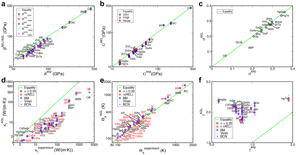
Figure 1: (a) Bulk modulus, (b) shear modulus, (c) Poisson ratio, (d) lattice thermal conductivity at 300K, (e) acoustic Debye temperature and (f) Grüneisen parameter of zincblende (AFLOW prototype: AB_cF8_216_c_a curtarolo:art121 ) and diamond (A_cF8_227_a curtarolo:art121 ) structure semiconductors.

The thermal properties Debye temperature, Grüneisen parameter and thermal conductivity calculated using AGL for this set of materials are compared to the experimental values taken from the literature in Table 2 and are also plotted in Fig. 1. For the Debye temperature, the experimental values $\theta^{\mathrm{exp}}$ are compared to $\theta_{\begin{subarray}{c}\scalebox{0.6}{D}\end{subarray}}^{\begin{subarray}{c}\scalebox{0.6}{AGL}\end{subarray}}$, $\theta_{\begin{subarray}{c}\scalebox{0.6}{D}\end{subarray}}^{\begin{subarray}{c}\scalebox{0.6}{BM}\end{subarray}}$, $\theta_{\begin{subarray}{c}\scalebox{0.6}{D}\end{subarray}}^{\begin{subarray}{c}\scalebox{0.6}{Vinet}\end{subarray}}$ and $\theta_{\begin{subarray}{c}\scalebox{0.6}{D}\end{subarray}}^{\begin{subarray}{c}\scalebox{0.6}{BCN}\end{subarray}}$ in Fig. 1(e), while the values for the empirical equations of state are provided in the supplementary information. Note that the $\theta^{\mathrm{exp}}$ values taken from Ref. slack, and Ref. Morelli_Slack_2006, are for $\theta_{\mathrm{a}}$, and generally are in good agreement with the $\theta_{\mathrm{a}}^{\begin{subarray}{c}\scalebox{0.6}{AGL}\end{subarray}}$ values. The values obtained using the numerical $E(V)$ fit and the three different equations of state are also in good agreement with each other, whereas the values of $\theta_{\begin{subarray}{c}\scalebox{0.6}{D}\end{subarray}}^{\begin{subarray}{c}\scalebox{0.6}{AGL}\end{subarray}}$ calculated using different $\sigma$ values differ significantly, indicating that for this property the value of $\sigma$ used is far more important than the equation of state used. The correlation between $\theta^{\mathrm{exp}}$ and the various AGL values is also very high, of the order of 0.999, and the RMSrD is low, of the order of 0.13.

Table 2: Thermal properties lattice thermal conductivity at 300K, Debye temperature and Grüneisen parameter of zincblende (AFLOW prototype: AB_cF8_216_c_a curtarolo:art121 ) and diamond (A_cF8_227_a curtarolo:art121 ) structure semiconductors, comparing the effect of using the calculated value of the Poisson ratio to the previous approximation of $\sigma=0.25$. The values listed for $\theta^{\mathrm{exp}}$ are $\theta_{\mathrm{a}}$, except 141K for HgTe which is $\theta_{\mathrm{D}}$ Snyder_jmatchem_2011 . Units: $\kappa$ in (W/(m$\cdot$K)), $\theta$ in (K).

Comp.	$\kappa^{\mathrm{exp}}$	$\kappa^{\begin{subarray}{c}\scalebox{0.6}{AGL}\end{subarray}}$	$\kappa^{\begin{subarray}{c}\scalebox{0.6}{AGL}\end{subarray}}$	$\theta^{\mathrm{exp}}$	$\theta_{\begin{subarray}{c}\scalebox{0.6}{D}\end{subarray}}^{\begin{subarray}{c}\scalebox{0.6}{AGL}\end{subarray}}$	$\theta_{\begin{subarray}{c}\scalebox{0.6}{D}\end{subarray}}^{\begin{subarray}{c}\scalebox{0.6}{AGL}\end{subarray}}$	$\theta_{\begin{subarray}{c}\scalebox{0.6}{D}\end{subarray}}^{\begin{subarray}{c}\scalebox{0.6}{AEL}\end{subarray}}$	$\gamma^{\mathrm{exp}}$	$\gamma^{\begin{subarray}{c}\scalebox{0.6}{AGL}\end{subarray}}$	$\gamma^{\begin{subarray}{c}\scalebox{0.6}{AGL}\end{subarray}}$
					($\theta_{\mathrm{a}}^{\begin{subarray}{c}\scalebox{0.6}{AGL}\end{subarray}}$)	($\theta_{\mathrm{a}}^{\begin{subarray}{c}\scalebox{0.6}{AGL}\end{subarray}}$)
		($\sigma=0.25$)curtarolo:art96			($\sigma=0.25$) curtarolo:art96				($\sigma=0.25$)curtarolo:art96
C	3000 Morelli_Slack_2006	169.1	419.9	1450 slack ; Morelli_Slack_2006	1536	2094	2222	0.75 Morelli_Slack_2006	1.74	1.77
					(1219)	(1662)		0.9 slack
SiC	360 Ioffe_Inst_DB	67.19	113.0	740 slack	928	1106	1143	0.76 slack	1.84	1.85
					(737)	(878)
Si	166 Morelli_Slack_2006	20.58	26.19	395 slack ; Morelli_Slack_2006	568	610	624	1.06 Morelli_Slack_2006	2.09	2.06
					(451)	(484)		0.56 slack
Ge	65 Morelli_Slack_2006	6.44	8.74	235 slack ; Morelli_Slack_2006	296	329	342	1.06 Morelli_Slack_2006	2.3	2.31
					(235)	(261)		0.76 slack
BN	760 Morelli_Slack_2006	138.4	281.6	1200 Morelli_Slack_2006	1409	1793	1887	0.7 Morelli_Slack_2006	1.73	1.75
					(1118)	(1423)
BP	350 Morelli_Slack_2006	52.56	105.0	670 slack ; Morelli_Slack_2006	811	1025	1062	0.75 Morelli_Slack_2006	1.78	1.79
					(644)	(814)
AlP	90 Landolt-Bornstein ; Spitzer_JPCS_1970	21.16	19.34	381 Morelli_Slack_2006	542	525	531	0.75 Morelli_Slack_2006	1.96	1.96
					(430)	(417)
AlAs	98 Morelli_Slack_2006	12.03	11.64	270 slack ; Morelli_Slack_2006	378	373	377	0.66 slack ; Morelli_Slack_2006	2.04	2.04
					(300)	(296)
AlSb	56 Morelli_Slack_2006	7.22	6.83	210 slack ; Morelli_Slack_2006	281	276	277	0.6 slack ; Morelli_Slack_2006	2.12	2.13
					(223)	(219)
GaP	100 Morelli_Slack_2006	11.76	13.34	275 slack ; Morelli_Slack_2006	396	412	423	0.75 Morelli_Slack_2006	2.15	2.15
					(314)	(327)		0.76 slack
GaAs	45 Morelli_Slack_2006	7.2	8.0	220 slack ; Morelli_Slack_2006	302	313	322	0.75 slack ; Morelli_Slack_2006	2.23	2.24
					(240)	(248)
GaSb	40 Morelli_Slack_2006	4.62	4.96	165 slack ; Morelli_Slack_2006	234	240	248	0.75 slack ; Morelli_Slack_2006	2.27	2.28
					(186)	(190)
InP	93 Morelli_Slack_2006	7.78	6.53	220 slack ; Morelli_Slack_2006	304	286	287	0.6 slack ; Morelli_Slack_2006	2.22	2.21
					(241)	(227)
InAs	30 Morelli_Slack_2006	5.36	4.33	165 slack ; Morelli_Slack_2006	246	229	231	0.57 slack ; Morelli_Slack_2006	2.26	2.26
					(195)	(182)
InSb	20 Morelli_Slack_2006	3.64	3.02	135 slack ; Morelli_Slack_2006	199	187	190	0.56 slack ; Morelli_Slack_2006	2.3	2.3
	16.5 Snyder_jmatchem_2011				(158)	(148)
ZnS	27 Morelli_Slack_2006	11.33	8.38	230 slack ; Morelli_Slack_2006	379	341	346	0.75 slack ; Morelli_Slack_2006	2.01	2.00
					(301)	(271)
ZnSe	19 Morelli_Slack_2006	7.46	5.44	190 slack ; Morelli_Slack_2006	290	260	263	0.75 slack ; Morelli_Slack_2006	2.07	2.06
	33 Snyder_jmatchem_2011				(230)	(206)
ZnTe	18 Morelli_Slack_2006	4.87	3.83	155 slack ; Morelli_Slack_2006	228	210	212	0.97 slack ; Morelli_Slack_2006	2.14	2.13
					(181)	(167)
CdSe	4.4 Snyder_jmatchem_2011	4.99	2.04	130 Morelli_Slack_2006	234	173	174	0.6 Morelli_Slack_2006	2.19	2.18
					(186)	(137)
CdTe	7.5 Morelli_Slack_2006	3.49	1.71	120 slack ; Morelli_Slack_2006	191	150	152	0.52 slack ; Morelli_Slack_2006	2.23	2.22
					(152)	(119)
HgSe	3 Whitsett_PRB_1973	3.22	1.32	110 slack	190	140	140	0.17 slack	2.4	2.38
					(151)	(111)
HgTe	2.5 Snyder_jmatchem_2011	2.36	1.21	141 Snyder_jmatchem_2011	162	129	130	1.9 Snyder_jmatchem_2011	2.46	2.45
				(100) slack	(129)	(102)

The experimental values $\gamma^{\mathrm{exp}}$ of the Grüneisen parameter are plotted against $\gamma^{\begin{subarray}{c}\scalebox{0.6}{AGL}\end{subarray}}$, $\gamma^{\begin{subarray}{c}\scalebox{0.6}{BM}\end{subarray}}$, $\gamma^{\begin{subarray}{c}\scalebox{0.6}{Vinet}\end{subarray}}$ and $\gamma^{\begin{subarray}{c}\scalebox{0.6}{BCN}\end{subarray}}$ in Fig. 1(f), and the values are listed in Table 2 and in the supplementary information. The very high RMSrD values (see Table 3) show that AGL has problems accurately predicting the Grüneisen parameter for this set of materials, as the calculated value is often 2 to 3 times larger than the experimental one. Note also that there are quite large differences between the values obtained for different equations of state, with $\gamma^{\begin{subarray}{c}\scalebox{0.6}{BCN}\end{subarray}}$ generally having the lowest values while $\gamma^{\begin{subarray}{c}\scalebox{0.6}{Vinet}\end{subarray}}$ has the highest values. On the other hand, in contrast to the case of $\theta_{\begin{subarray}{c}\scalebox{0.6}{D}\end{subarray}}^{\begin{subarray}{c}\scalebox{0.6}{AGL}\end{subarray}}$, the value of $\sigma$ used makes little difference to the value of $\gamma^{\begin{subarray}{c}\scalebox{0.6}{AGL}\end{subarray}}$. The correlations between $\gamma^{\mathrm{exp}}$ and the AGL values, as shown in Table 3, are also quite poor, with no value higher than 0.2 for the Pearson correlations, and negative Spearman correlations.

The experimental thermal conductivity $\kappa^{\mathrm{exp}}$ is compared in Fig. 1(d) to the thermal conductivities calculated with AGL using the Leibfried-Schlömann equation (Eq. (II.5)): $\kappa^{\begin{subarray}{c}\scalebox{0.6}{AGL}\end{subarray}}$, $\kappa^{\begin{subarray}{c}\scalebox{0.6}{BM}\end{subarray}}$, $\kappa^{\begin{subarray}{c}\scalebox{0.6}{Vinet}\end{subarray}}$ and $\kappa^{\begin{subarray}{c}\scalebox{0.6}{BCN}\end{subarray}}$, while the values are listed in Table 2 and in the supplementary information. The absolute agreement between the AGL values and $\kappa^{\mathrm{exp}}$ is quite poor, with RMSrD values of the order of 0.8 and discrepancies of tens, or even hundreds, of percent quite common. Considerable disagreements also exist between different experimental reports of these properties, in almost all cases where they exist. Unfortunately, the scarcity of experimental data from different sources on the thermal properties of these materials prevents reaching definite conclusions regarding the true values of these properties. The available data can thus only be considered as a rough indication of their order of magnitude.

The Pearson correlations between the AGL calculated thermal conductivity values and the experimental values are high, ranging from $0.871$ to $0.932$, while the Spearman correlations are even higher, ranging from $0.905$ to $0.954$, as shown in Table 3. In particular, note that using the $\sigma^{\begin{subarray}{c}\scalebox{0.6}{AEL}\end{subarray}}$ in the AGL calculations improves the correlations by about 5%, from $0.878$ to $0.927$ and from $0.905$ to $0.954$. For the different equations of state, $\kappa^{\begin{subarray}{c}\scalebox{0.6}{AGL}\end{subarray}}$ and $\kappa^{\begin{subarray}{c}\scalebox{0.6}{BCN}\end{subarray}}$ appear to correlate better with $\kappa^{\mathrm{exp}}$ than $\kappa^{\begin{subarray}{c}\scalebox{0.6}{BM}\end{subarray}}$ and $\kappa^{\begin{subarray}{c}\scalebox{0.6}{Vinet}\end{subarray}}$ for this set of materials.

Table 3: Correlations and deviations between experimental values and AEL and AGL results for elastic and thermal properties for zincblende and diamond structure semiconductors.

Property	Pearson	Spearman	RMSrD
	(Linear)	(Rank Order)
$\kappa^{\mathrm{exp}}$ vs. $\kappa^{\begin{subarray}{c}\scalebox{0.6}{AGL}\end{subarray}}$ ($\sigma=0.25$) curtarolo:art96	0.878	0.905	0.776
$\kappa^{\mathrm{exp}}$ vs. $\kappa^{\begin{subarray}{c}\scalebox{0.6}{AGL}\end{subarray}}$	0.927	0.95	0.796
$\kappa^{\mathrm{exp}}$ vs. $\kappa^{\begin{subarray}{c}\scalebox{0.6}{BM}\end{subarray}}$	0.871	0.954	0.787
$\kappa^{\mathrm{exp}}$ vs. $\kappa^{\begin{subarray}{c}\scalebox{0.6}{Vinet}\end{subarray}}$	0.908	0.954	0.815
$\kappa^{\mathrm{exp}}$ vs. $\kappa^{\begin{subarray}{c}\scalebox{0.6}{BCN}\end{subarray}}$	0.932	0.954	0.771
$\theta_{\mathrm{a}}^{\mathrm{exp}}$ vs. $\theta_{\mathrm{a}}^{\begin{subarray}{c}\scalebox{0.6}{AGL}\end{subarray}}$ ($\sigma=0.25$) curtarolo:art96	0.995	0.984	0.200
$\theta_{\mathrm{a}}^{\mathrm{exp}}$ vs. $\theta_{\mathrm{a}}^{\begin{subarray}{c}\scalebox{0.6}{AGL}\end{subarray}}$	0.999	0.998	0.132
$\theta_{\mathrm{a}}^{\mathrm{exp}}$ vs. $\theta_{\mathrm{a}}^{\begin{subarray}{c}\scalebox{0.6}{BM}\end{subarray}}$	0.999	0.998	0.132
$\theta_{\mathrm{a}}^{\mathrm{exp}}$ vs. $\theta_{\mathrm{a}}^{\begin{subarray}{c}\scalebox{0.6}{Vinet}\end{subarray}}$	0.999	0.998	0.127
$\theta_{\mathrm{a}}^{\mathrm{exp}}$ vs. $\theta_{\mathrm{a}}^{\begin{subarray}{c}\scalebox{0.6}{BCN}\end{subarray}}$	0.999	0.998	0.136
$\gamma^{\mathrm{exp}}$ vs. $\gamma^{\begin{subarray}{c}\scalebox{0.6}{AGL}\end{subarray}}$ ($\sigma=0.25$) curtarolo:art96	0.137	-0.187	3.51
$\gamma^{\mathrm{exp}}$ vs. $\gamma^{\begin{subarray}{c}\scalebox{0.6}{AGL}\end{subarray}}$	0.145	-0.165	3.49
$\gamma^{\mathrm{exp}}$ vs. $\gamma^{\begin{subarray}{c}\scalebox{0.6}{BM}\end{subarray}}$	0.169	-0.178	3.41
$\gamma^{\mathrm{exp}}$ vs. $\gamma^{\begin{subarray}{c}\scalebox{0.6}{Vinet}\end{subarray}}$	0.171	-0.234	3.63
$\gamma^{\mathrm{exp}}$ vs. $\gamma^{\begin{subarray}{c}\scalebox{0.6}{BCN}\end{subarray}}$	0.144	-0.207	3.32
$B^{\mathrm{exp}}$ vs. $B_{\begin{subarray}{c}\scalebox{0.6}{VRH}\end{subarray}}^{\begin{subarray}{c}\scalebox{0.6}{AEL}\end{subarray}}$	0.999	0.992	0.130
$B^{\mathrm{exp}}$ vs. $B_{\begin{subarray}{c}\scalebox{0.6}{Static}\end{subarray}}^{\begin{subarray}{c}\scalebox{0.6}{AGL}\end{subarray}}$	0.999	0.986	0.201
$B^{\mathrm{exp}}$ vs. $B_{\begin{subarray}{c}\scalebox{0.6}{Static}\end{subarray}}^{\begin{subarray}{c}\scalebox{0.6}{BM}\end{subarray}}$	0.999	0.986	0.189
$B^{\mathrm{exp}}$ vs. $B_{\begin{subarray}{c}\scalebox{0.6}{Static}\end{subarray}}^{\begin{subarray}{c}\scalebox{0.6}{Vinet}\end{subarray}}$	0.999	0.986	0.205
$B^{\mathrm{exp}}$ vs. $B_{\begin{subarray}{c}\scalebox{0.6}{Static}\end{subarray}}^{\begin{subarray}{c}\scalebox{0.6}{BCN}\end{subarray}}$	0.999	0.986	0.185
$G^{\mathrm{exp}}$ vs. $G_{\begin{subarray}{c}\scalebox{0.6}{VRH}\end{subarray}}^{\begin{subarray}{c}\scalebox{0.6}{AEL}\end{subarray}}$	0.998	0.980	0.111
$G^{\mathrm{exp}}$ vs. $G_{\begin{subarray}{c}\scalebox{0.6}{Voigt}\end{subarray}}^{\begin{subarray}{c}\scalebox{0.6}{AEL}\end{subarray}}$	0.998	0.980	0.093
$G^{\mathrm{exp}}$ vs. $G_{\begin{subarray}{c}\scalebox{0.6}{Reuss}\end{subarray}}^{\begin{subarray}{c}\scalebox{0.6}{AEL}\end{subarray}}$	0.998	0.980	0.152
$\sigma^{\mathrm{exp}}$ vs. $\sigma^{\begin{subarray}{c}\scalebox{0.6}{AEL}\end{subarray}}$	0.977	0.982	0.095

As we noted in our previous work on AGL curtarolo:art96 , some of the inaccuracy in the thermal conductivity results may be due to the inability of the Leibfried-Schlömann equation to fully describe effects such as the suppression of phonon-phonon scattering due to large gaps between the branches of the phonon dispersion Lindsay_PRL_2013 . This can be seen from the thermal conductivity values shown in Table 2.2 of Ref. Morelli_Slack_2006, calculated using the experimental values of $\theta_{\mathrm{a}}$ and $\gamma$ in the Leibfried-Schlömann equation. There are large discrepancies in certain cases such as diamond, while the Pearson and Spearman correlations of $0.932$ and $0.941$ respectively are very similar to the correlations we calculated using the AGL evaluations of $\theta_{\mathrm{a}}$ and $\gamma$.

Thus, the unsatisfactory quantitative reproduction of these quantities by the Debye quasi-harmonic model has little impact on its effectiveness as a screening tool for identifying high or low thermal conductivity materials. The model can be used when these experimental values are unavailable to help determine the relative values of these quantities and for ranking materials conductivity.

III.2 Rocksalt structure materials

The mechanical and thermal properties were calculated for a set of materials with the rocksalt structure (spacegroup: Fm$\overline{3}$m, $\#$225; Pearson symbol: cF8; AFLOW Prototype: AB_cF8_225_a_b curtarolo:art121 ). This is the same set of materials as in Table II of Ref. curtarolo:art96, , which in turn are from the sets in Table III of Ref. slack, and Table 2.1 of Ref. Morelli_Slack_2006, .

The elastic properties of bulk modulus, shear modulus and Poisson ratio, as calculated using AEL and AGL are shown in Table 4 and Fig. 2, together with experimental values from the literature where available. As can be seen from the results in Table 4 and Fig. 2(a), for this set of materials the $B_{\begin{subarray}{c}\scalebox{0.6}{VRH}\end{subarray}}^{\begin{subarray}{c}\scalebox{0.6}{AEL}\end{subarray}}$ values are closest to experiment, with an RMSrD of 0.078. The AGL values from both the numerical fit and the empirical equations of state are generally very similar to each other, while being slightly less than the $B_{\begin{subarray}{c}\scalebox{0.6}{VRH}\end{subarray}}^{\begin{subarray}{c}\scalebox{0.6}{AEL}\end{subarray}}$ values.

Table 4: Mechanical properties bulk modulus, shear modulus and Poisson ratio of rocksalt (AFLOW Prototype: AB_cF8_225_a_b curtarolo:art121 ) structure semiconductors. “N/A” = Not available for that source. Units: $B$ and $G$ in (GPa).

Comp.	$B^{\mathrm{exp}}$	$B_{\begin{subarray}{c}\scalebox{0.6}{VRH}\end{subarray}}^{\begin{subarray}{c}\scalebox{0.6}{AEL}\end{subarray}}$	$B_{\begin{subarray}{c}\scalebox{0.6}{VRH}\end{subarray}}^{\begin{subarray}{c}\scalebox{0.6}{MP}\end{subarray}}$	$B_{\begin{subarray}{c}\scalebox{0.6}{Static}\end{subarray}}^{\begin{subarray}{c}\scalebox{0.6}{AGL}\end{subarray}}$	$B_{\begin{subarray}{c}\scalebox{0.6}{Static}\end{subarray}}^{\begin{subarray}{c}\scalebox{0.6}{BM}\end{subarray}}$	$B_{\begin{subarray}{c}\scalebox{0.6}{Static}\end{subarray}}^{\begin{subarray}{c}\scalebox{0.6}{Vinet}\end{subarray}}$	$B_{\begin{subarray}{c}\scalebox{0.6}{Static}\end{subarray}}^{\begin{subarray}{c}\scalebox{0.6}{BCN}\end{subarray}}$	$G^{\mathrm{exp}}$	$G_{\begin{subarray}{c}\scalebox{0.6}{Voigt}\end{subarray}}^{\begin{subarray}{c}\scalebox{0.6}{AEL}\end{subarray}}$	$G_{\begin{subarray}{c}\scalebox{0.6}{Reuss}\end{subarray}}^{\begin{subarray}{c}\scalebox{0.6}{AEL}\end{subarray}}$	$G_{\begin{subarray}{c}\scalebox{0.6}{VRH}\end{subarray}}^{\begin{subarray}{c}\scalebox{0.6}{AEL}\end{subarray}}$	$G_{\begin{subarray}{c}\scalebox{0.6}{VRH}\end{subarray}}^{\begin{subarray}{c}\scalebox{0.6}{MP}\end{subarray}}$	$\sigma^{\mathrm{exp}}$	$\sigma^{\begin{subarray}{c}\scalebox{0.6}{AEL}\end{subarray}}$	$\sigma^{\begin{subarray}{c}\scalebox{0.6}{MP}\end{subarray}}$
LiH	33.7 Laplaze_ElasticLiH_SSC_1976	37.7	36.1	29.5	29.0	27.7	31.4	36.0 Laplaze_ElasticLiH_SSC_1976	43.4	42.3	42.8	42.9	0.106 Laplaze_ElasticLiH_SSC_1976	0.088	0.07
LiF	69.6 Haussuhl_ElasticRocksalt_ZP_1960	70.4	69.9	58.6	59.9	57.5	61.2	48.8 Haussuhl_ElasticRocksalt_ZP_1960	46.4	45.8	46.1	50.9	0.216 Haussuhl_ElasticRocksalt_ZP_1960	0.231	0.21
NaF	48.5 Haussuhl_ElasticRocksalt_ZP_1960	46.9	47.6	38.7	38.6	36.8	39.3	31.2 Haussuhl_ElasticRocksalt_ZP_1960	29.5	28.4	28.9	30.0	0.236 Haussuhl_ElasticRocksalt_ZP_1960	0.244	0.24
NaCl	25.1 Haussuhl_ElasticRocksalt_ZP_1960	24.9	22.6	20.0	20.5	19.2	20.7	14.6 Haussuhl_ElasticRocksalt_ZP_1960	14.0	12.9	13.5	14.3	0.255 Haussuhl_ElasticRocksalt_ZP_1960	0.271	0.24
NaBr	20.6 Haussuhl_ElasticRocksalt_ZP_1960	20.5	27.1	16.3	16.9	15.7	16.9	11.6 Haussuhl_ElasticRocksalt_ZP_1960	11.0	9.9	10.4	11.6	0.264 Haussuhl_ElasticRocksalt_ZP_1960	0.283	0.31
NaI	15.95 Haussuhl_ElasticRocksalt_ZP_1960	16.4	15.8	12.6	13.2	12.2	13.1	8.59 Haussuhl_ElasticRocksalt_ZP_1960	8.35	7.31	7.83	8.47	0.272 Haussuhl_ElasticRocksalt_ZP_1960	0.295	0.27
KF	31.6 Haussuhl_ElasticRocksalt_ZP_1960	29.9	28.9	25.1	24.2	22.9	24.7	16.7 Haussuhl_ElasticRocksalt_ZP_1960	16.5	15.4	15.9	16.5	0.275 Haussuhl_ElasticRocksalt_ZP_1960	0.274	0.26
KCl	18.2 Haussuhl_ElasticRocksalt_ZP_1960	16.7	15.8	13.8	13.7	12.7	13.6	9.51 Haussuhl_ElasticRocksalt_ZP_1960	10.1	8.51	9.30	9.24	0.277 Haussuhl_ElasticRocksalt_ZP_1960	0.265	0.26
KBr	15.4 Haussuhl_ElasticRocksalt_ZP_1960	13.8	21.6	11.1	11.4	10.5	11.2	7.85 Haussuhl_ElasticRocksalt_ZP_1960	8.14	6.46	7.30	7.33	0.282 Haussuhl_ElasticRocksalt_ZP_1960	0.276	0.35
KI	12.2 Haussuhl_ElasticRocksalt_ZP_1960	10.9	9.52	8.54	9.03	8.28	8.84	5.96 Haussuhl_ElasticRocksalt_ZP_1960	6.05	4.39	5.22	5.55	0.290 Haussuhl_ElasticRocksalt_ZP_1960	0.294	0.26
RbCl	16.2 Haussuhl_ElasticRocksalt_ZP_1960	14.3	14.6	12.1	11.8	11.0	11.8	7.63 Haussuhl_ElasticRocksalt_ZP_1960	8.06	6.41	7.24	7.67	0.297 Haussuhl_ElasticRocksalt_ZP_1960	0.284	0.28
RbBr	13.8 Haussuhl_ElasticRocksalt_ZP_1960	12.6	13.8	10.3	9.72	9.06	9.67	6.46 Haussuhl_ElasticRocksalt_ZP_1960	7.12	5.24	6.18	6.46	0.298 Haussuhl_ElasticRocksalt_ZP_1960	0.289	0.3
RbI	11.1 Haussuhl_ElasticRocksalt_ZP_1960	9.90	9.66	8.01	7.74	7.12	7.54	5.03 Haussuhl_ElasticRocksalt_ZP_1960	5.50	3.65	4.57	4.63	0.303 Haussuhl_ElasticRocksalt_ZP_1960	0.300	0.29
AgCl	44.0 Hughes_ElasticAgCl_PRB_1996	40.6	N/A	33.7	34.1	33.0	34.7	8.03 Hughes_ElasticAgCl_PRB_1996	8.68	8.66	8.67	N/A	0.414 Hughes_ElasticAgCl_PRB_1996	0.400	N/A
MgO	164 Sumino_ElasticMgO_JPE_1976	152	152	142	142	140	144	131 Sumino_ElasticMgO_JPE_1976	119	115	117	119	0.185 Sumino_ElasticMgO_JPE_1976	0.194	0.19
CaO	113 Chang_ElasticCaSrBaO_JPCS_1977	105	105	99.6	100	98.7	101	81.0 Chang_ElasticCaSrBaO_JPCS_1977	73.7	73.7	73.7	74.2	0.210 Chang_ElasticCaSrBaO_JPCS_1977	0.216	0.21
SrO	91.2 Chang_ElasticCaSrBaO_JPCS_1977	84.7	87.4	80.0	80.2	79.1	80.8	58.7 Chang_ElasticCaSrBaO_JPCS_1977	55.1	55.0	55.1	56.0	0.235 Chang_ElasticCaSrBaO_JPCS_1977	0.233	0.24
BaO	75.4 Chang_ElasticCaSrBaO_JPCS_1977	69.1	68.4	64.6	64.3	63.0	64.6	35.4 Chang_ElasticCaSrBaO_JPCS_1977	36.4	36.4	36.4	37.8	0.297 Chang_ElasticCaSrBaO_JPCS_1977	0.276	0.27
PbS	52.9 Semiconductors_BasicData_Springer ; Peresada_ElasticPbS_PSSa_1976	53.5	N/A	49.9	50.8	50.0	51.0	27.9 Semiconductors_BasicData_Springer ; Peresada_ElasticPbS_PSSa_1976	34.0	26.8	30.4	N/A	0.276 Semiconductors_BasicData_Springer ; Peresada_ElasticPbS_PSSa_1976	0.261	N/A
PbSe	54.1 Semiconductors_BasicData_Springer ; Lippmann_ElasticPbSe_PSSa_1971	47.7	N/A	43.9	44.8	43.9	44.9	26.2 Semiconductors_BasicData_Springer ; Lippmann_ElasticPbSe_PSSa_1971	31.7	23.6	27.6	N/A	0.291 Semiconductors_BasicData_Springer ; Lippmann_ElasticPbSe_PSSa_1971	0.257	N/A
PbTe	39.8 Semiconductors_BasicData_Springer ; Miller_ElasticPbTe_JPCSS_1981	39.5	N/A	36.4	36.6	35.8	36.8	23.1 Semiconductors_BasicData_Springer ; Miller_ElasticPbTe_JPCSS_1981	28.7	19.8	24.3	N/A	0.256 Semiconductors_BasicData_Springer ; Miller_ElasticPbTe_JPCSS_1981	0.245	N/A
SnTe	37.8 Semiconductors_BasicData_Springer ; Seddon_ElasticSnTe_SSC_1976	40.4	39.6	38.1	38.4	37.6	38.6	20.8 Semiconductors_BasicData_Springer ; Seddon_ElasticSnTe_SSC_1976	31.4	22.0	26.7	27.6	0.267 Semiconductors_BasicData_Springer ; Seddon_ElasticSnTe_SSC_1976	0.229	0.22

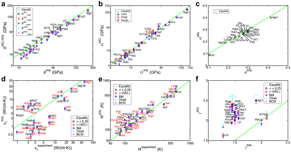
Figure 2: (a) Bulk modulus, (b) shear modulus, (c) Poisson ratio, (d) lattice thermal conductivity at 300K, (e) Debye temperature and (f) Grüneisen parameter of rocksalt structure (AFLOW Prototype: AB_cF8_225_a_b curtarolo:art121 ) semiconductors. The Debye temperatures plotted in (b) are $\theta_{\mathrm{a}}$, except for SnTe where $\theta_{\mathrm{D}}$ is quoted in Ref. Snyder_jmatchem_2011, .

For the shear modulus, the experimental values $G^{\mathrm{exp}}$ are compared to the AEL values $G_{\begin{subarray}{c}\scalebox{0.6}{Voigt}\end{subarray}}^{\begin{subarray}{c}\scalebox{0.6}{AEL}\end{subarray}}$, $G_{\begin{subarray}{c}\scalebox{0.6}{Reuss}\end{subarray}}^{\begin{subarray}{c}\scalebox{0.6}{AEL}\end{subarray}}$ and $G_{\begin{subarray}{c}\scalebox{0.6}{VRH}\end{subarray}}^{\begin{subarray}{c}\scalebox{0.6}{AEL}\end{subarray}}$. As can be seen from the values in Table 4 and Fig. 2(b), the agreement with the experimental values is generally good with an RMSrD of 0.105 for $G_{\begin{subarray}{c}\scalebox{0.6}{VRH}\end{subarray}}^{\begin{subarray}{c}\scalebox{0.6}{AEL}\end{subarray}}$, with the Voigt approximation tending to overestimate and the Reuss approximation tending to underestimate, as would be expected. The experimental values of the Poisson ratio $\sigma^{\mathrm{exp}}$ and the AEL values $\sigma^{\begin{subarray}{c}\scalebox{0.6}{AEL}\end{subarray}}$ (Eq. (8)) are also shown in Table 4 and Fig. 2(c), and the values are generally in good agreement. The Pearson (i.e. linear, Eq. (40)) and Spearman (i.e. rank order, Eq. (41)) correlations between all of the the AEL-AGL elastic property values and experiment are shown in Table 6, and are generally very high for all of these properties, ranging from 0.959 and 0.827 respectively for $\sigma^{\mathrm{exp}}$ vs. $\sigma^{\begin{subarray}{c}\scalebox{0.6}{AEL}\end{subarray}}$, up to 0.998 and 0.995 for $B^{\mathrm{exp}}$ vs. $B_{\begin{subarray}{c}\scalebox{0.6}{VRH}\end{subarray}}^{\begin{subarray}{c}\scalebox{0.6}{AEL}\end{subarray}}$. These very high correlation values demonstrate the validity of using the AEL-AGL methodology to predict the elastic and mechanical properties of materials.

The values of $B_{\begin{subarray}{c}\scalebox{0.6}{VRH}\end{subarray}}^{\begin{subarray}{c}\scalebox{0.6}{MP}\end{subarray}}$, $G_{\begin{subarray}{c}\scalebox{0.6}{VRH}\end{subarray}}^{\begin{subarray}{c}\scalebox{0.6}{MP}\end{subarray}}$ and $\sigma^{\begin{subarray}{c}\scalebox{0.6}{MP}\end{subarray}}$ for rocksalt structure materials are also shown in Table 4, where available. The Pearson correlations for the experimental results with the available values of $B_{\begin{subarray}{c}\scalebox{0.6}{VRH}\end{subarray}}^{\begin{subarray}{c}\scalebox{0.6}{MP}\end{subarray}}$, $G_{\begin{subarray}{c}\scalebox{0.6}{VRH}\end{subarray}}^{\begin{subarray}{c}\scalebox{0.6}{MP}\end{subarray}}$ and $\sigma^{\begin{subarray}{c}\scalebox{0.6}{MP}\end{subarray}}$ were calculated to be 0.997, 0.994 and 0.890, respectively, while the respective Spearman correlations were 0.979, 0.998 and 0.817, and the RMSrD values were 0.153, 0.105 and 0.126. For comparison, the corresponding Pearson correlations for the same subset of materials for $B_{\begin{subarray}{c}\scalebox{0.6}{VRH}\end{subarray}}^{\begin{subarray}{c}\scalebox{0.6}{AEL}\end{subarray}}$, $G_{\begin{subarray}{c}\scalebox{0.6}{VRH}\end{subarray}}^{\begin{subarray}{c}\scalebox{0.6}{AEL}\end{subarray}}$ and $\sigma^{\begin{subarray}{c}\scalebox{0.6}{AEL}\end{subarray}}$ are 0.998, 0.995, and 0.951 respectively, while the respective Spearman correlations were 0.996, 1.0 and 0.843, and the RMSrD values were 0.079, 0.111 and 0.071. These correlation values are very similar, and the general close agreement for the results for the values of $B_{\begin{subarray}{c}\scalebox{0.6}{VRH}\end{subarray}}^{\begin{subarray}{c}\scalebox{0.6}{AEL}\end{subarray}}$, $G_{\begin{subarray}{c}\scalebox{0.6}{VRH}\end{subarray}}^{\begin{subarray}{c}\scalebox{0.6}{AEL}\end{subarray}}$ and $\sigma^{\begin{subarray}{c}\scalebox{0.6}{AEL}\end{subarray}}$ with those of $B_{\begin{subarray}{c}\scalebox{0.6}{VRH}\end{subarray}}^{\begin{subarray}{c}\scalebox{0.6}{MP}\end{subarray}}$, $G_{\begin{subarray}{c}\scalebox{0.6}{VRH}\end{subarray}}^{\begin{subarray}{c}\scalebox{0.6}{MP}\end{subarray}}$ and $\sigma^{\begin{subarray}{c}\scalebox{0.6}{MP}\end{subarray}}$ demonstrate that the small differences in the parameters used for the DFT calculations make little difference to the results, indicating that the parameter set used here is robust for high-throughput calculations.

The thermal properties of Debye temperature, Grüneisen parameter and thermal conductivity calculated using AGL are compared to the experimental values taken from the literature in Table 5 and are also plotted in Fig. 2. For the Debye temperature, the experimental values $\theta^{\mathrm{exp}}$ are compared to $\theta_{\begin{subarray}{c}\scalebox{0.6}{D}\end{subarray}}^{\begin{subarray}{c}\scalebox{0.6}{AGL}\end{subarray}}$, $\theta_{\begin{subarray}{c}\scalebox{0.6}{D}\end{subarray}}^{\begin{subarray}{c}\scalebox{0.6}{BM}\end{subarray}}$, $\theta_{\begin{subarray}{c}\scalebox{0.6}{D}\end{subarray}}^{\begin{subarray}{c}\scalebox{0.6}{Vinet}\end{subarray}}$ and $\theta_{\begin{subarray}{c}\scalebox{0.6}{D}\end{subarray}}^{\begin{subarray}{c}\scalebox{0.6}{BCN}\end{subarray}}$ in Fig. 2(e), while the actual values for the empirical equations of state are provided in the supplementary information. Note that the $\theta^{\mathrm{exp}}$ values taken from Ref. slack, and Ref. Morelli_Slack_2006, are for $\theta_{\mathrm{a}}$, and generally are in good agreement with the $\theta_{\mathrm{a}}^{\begin{subarray}{c}\scalebox{0.6}{AGL}\end{subarray}}$ values. The values obtained using the numerical $E(V)$ fit and the three different equations of state are also in good agreement with each other, whereas the values of $\theta_{\begin{subarray}{c}\scalebox{0.6}{D}\end{subarray}}^{\begin{subarray}{c}\scalebox{0.6}{AGL}\end{subarray}}$ calculated using different $\sigma$ values differ significantly, indicating that, as in the case of the zincblende and diamond structures, the value of $\sigma$ used is far more important for this property than the equation of state used. The correlation between $\theta^{\mathrm{exp}}$ and the various AGL values is also quite high, of the order of 0.98 for the Pearson correlation and 0.92 for the Spearman correlation.

Table 5: Thermal properties lattice thermal conductivity at 300K, Debye temperature and Grüneisen parameter of rocksalt structure (AFLOW Prototype: AB_cF8_225_a_b curtarolo:art121 ) semiconductors, comparing the effect of using the calculated value of the Poisson ratio to previous approximation of $\sigma=0.25$. The values listed for $\theta^{\mathrm{exp}}$ are $\theta_{\mathrm{a}}$, except 155K for SnTe which is $\theta_{\mathrm{D}}$ Snyder_jmatchem_2011 . “N/A” = Not available for that source. Units: $\kappa$ in (W/(m$\cdot$K)), $\theta$ in (K).

Comp.	$\kappa^{\mathrm{exp}}$	$\kappa^{\begin{subarray}{c}\scalebox{0.6}{AGL}\end{subarray}}$	$\kappa^{\begin{subarray}{c}\scalebox{0.6}{AGL}\end{subarray}}$	$\theta^{\mathrm{exp}}$	$\theta_{\begin{subarray}{c}\scalebox{0.6}{D}\end{subarray}}^{\begin{subarray}{c}\scalebox{0.6}{AGL}\end{subarray}}$	$\theta_{\begin{subarray}{c}\scalebox{0.6}{D}\end{subarray}}^{\begin{subarray}{c}\scalebox{0.6}{AGL}\end{subarray}}$	$\theta_{\begin{subarray}{c}\scalebox{0.6}{D}\end{subarray}}^{\begin{subarray}{c}\scalebox{0.6}{AEL}\end{subarray}}$	$\gamma^{\mathrm{exp}}$	$\gamma^{\begin{subarray}{c}\scalebox{0.6}{AGL}\end{subarray}}$	$\gamma^{\begin{subarray}{c}\scalebox{0.6}{AGL}\end{subarray}}$
					($\theta_{\mathrm{a}}^{\begin{subarray}{c}\scalebox{0.6}{AGL}\end{subarray}}$)	($\theta_{\mathrm{a}}^{\begin{subarray}{c}\scalebox{0.6}{AGL}\end{subarray}}$)
		($\sigma=0.25$) curtarolo:art96			($\sigma=0.25$) curtarolo:art96				($\sigma=0.25$) curtarolo:art96
LiH	15 Morelli_Slack_2006	8.58	18.6	615 slack ; Morelli_Slack_2006	743	962	1175	1.28 slack ; Morelli_Slack_2006	1.62	1.66
					(590)	(764)
LiF	17.6 Morelli_Slack_2006	8.71	9.96	500 slack ; Morelli_Slack_2006	591	617	681	1.5 slack ; Morelli_Slack_2006	2.02	2.03
					(469)	(490)
NaF	18.4 Morelli_Slack_2006	4.52	4.67	395 slack ; Morelli_Slack_2006	411	416	455	1.5 slack ; Morelli_Slack_2006	2.2	2.21
					(326)	(330)
NaCl	7.1 Morelli_Slack_2006	2.43	2.12	220 slack ; Morelli_Slack_2006	284	271	289	1.56 slack ; Morelli_Slack_2006	2.23	2.23
					(225)	(215)
NaBr	2.8 Morelli_Slack_2006	1.66	1.33	150 slack ; Morelli_Slack_2006	203	188	198	1.5 slack ; Morelli_Slack_2006	2.22	2.22
					(161)	(149)
NaI	1.8 Morelli_Slack_2006	1.17	0.851	100 slack ; Morelli_Slack_2006	156	140	147	1.56 slack ; Morelli_Slack_2006	2.23	2.23
					(124)	(111)
KF	N/A	2.68	2.21	235 slack ; Morelli_Slack_2006	305	288	309	1.52 slack ; Morelli_Slack_2006	2.29	2.32
					(242)	(229)
KCl	7.1 Morelli_Slack_2006	1.4	1.25	172 slack ; Morelli_Slack_2006	220	213	226	1.45 slack ; Morelli_Slack_2006	2.38	2.40
					(175)	(169)
KBr	3.4 Morelli_Slack_2006	1.0	0.842	117 slack ; Morelli_Slack_2006	165	156	162	1.45 slack ; Morelli_Slack_2006	2.37	2.37
					(131)	(124)
KI	2.6 Morelli_Slack_2006	0.72	0.525	87 slack ; Morelli_Slack_2006	129	116	120	1.45 slack ; Morelli_Slack_2006	2.35	2.35
					(102)	(92)
RbCl	2.8 Morelli_Slack_2006	1.09	0.837	124 slack ; Morelli_Slack_2006	168	155	160	1.45 slack ; Morelli_Slack_2006	2.34	2.37
					(133)	(123)
RbBr	3.8 Morelli_Slack_2006	0.76	0.558	105 slack ; Morelli_Slack_2006	134	122	129	1.45 slack ; Morelli_Slack_2006	2.40	2.43
					(106)	(97)
RbI	2.3 Morelli_Slack_2006	0.52	0.368	84 slack ; Morelli_Slack_2006	109	97	102	1.41 slack ; Morelli_Slack_2006	2.47	2.47
					(87)	(77)
AgCl	1.0 Landolt-Bornstein ; Maqsood_IJT_2003	2.58	0.613	124 slack	235	145	148	1.9 slack	2.5	2.49
					(187)	(115)
MgO	60 Morelli_Slack_2006	31.9	44.5	600 slack ; Morelli_Slack_2006	758	849	890	1.44 slack ; Morelli_Slack_2006	1.95	1.96
					(602)	(674)
CaO	27 Morelli_Slack_2006	19.5	24.3	450 slack ; Morelli_Slack_2006	578	620	638	1.57 slack ; Morelli_Slack_2006	2.07	2.06
					(459)	(492)
SrO	12 Morelli_Slack_2006	12.5	13.4	270 slack ; Morelli_Slack_2006	399	413	421	1.52 slack ; Morelli_Slack_2006	2.09	2.13
					(317)	(328)
BaO	2.3 Morelli_Slack_2006	8.88	7.10	183 slack ; Morelli_Slack_2006	305	288	292	1.5 slack ; Morelli_Slack_2006	2.09	2.14
					(242)	(229)
PbS	2.9 Morelli_Slack_2006	6.48	6.11	115 slack ; Morelli_Slack_2006	226	220	221	2.0 slack ; Morelli_Slack_2006	2.02	2.00
					(179)	(175)
PbSe	2.0 Morelli_Slack_2006	4.88	4.81	100 Morelli_Slack_2006	197	194	196	1.5 Morelli_Slack_2006	2.1	2.07
					(156)	(154)
PbTe	2.5 Morelli_Slack_2006	4.15	4.07	105 slack ; Morelli_Slack_2006	170	172	175	1.45 slack ; Morelli_Slack_2006	2.04	2.09
					(135)	(137)
SnTe	1.5 Snyder_jmatchem_2011	4.46	5.24	155 Snyder_jmatchem_2011	202	210	212	2.1 Snyder_jmatchem_2011	2.15	2.11
					(160)	(167)

The experimental values $\gamma^{\mathrm{exp}}$ of the Grüneisen parameter are plotted against $\gamma^{\begin{subarray}{c}\scalebox{0.6}{AGL}\end{subarray}}$, $\gamma^{\begin{subarray}{c}\scalebox{0.6}{BM}\end{subarray}}$, $\gamma^{\begin{subarray}{c}\scalebox{0.6}{Vinet}\end{subarray}}$ and $\gamma^{\begin{subarray}{c}\scalebox{0.6}{BCN}\end{subarray}}$ in Fig. 2(f), and the values are listed in Table 5 and in the supplementary information. These results show that AGL has problems accurately predicting the Grüneisen parameter for this set of materials as well, as the calculated values are often 30% to 50% larger than the experimental ones and the RMSrD values are of the order of 0.5. Note also that there are quite large differences between the values obtained for different equations of state, with $\gamma^{\begin{subarray}{c}\scalebox{0.6}{BCN}\end{subarray}}$ generally having the lowest values while $\gamma^{\begin{subarray}{c}\scalebox{0.6}{Vinet}\end{subarray}}$ has the highest values, a similar pattern to that seen above for the zincblende and diamond structure materials. On the other hand, in contrast to the case of $\theta_{\begin{subarray}{c}\scalebox{0.6}{D}\end{subarray}}^{\begin{subarray}{c}\scalebox{0.6}{AGL}\end{subarray}}$, the value of $\sigma$ used makes little difference to the value of $\gamma^{\begin{subarray}{c}\scalebox{0.6}{AGL}\end{subarray}}$. The correlation values between $\gamma^{\mathrm{exp}}$ and the AGL values, as shown in Table 6, are also quite poor, with values ranging from -0.098 to 0.118 for the Pearson correlations, and negative values for the Spearman correlations.

The experimental thermal conductivity $\kappa^{\mathrm{exp}}$ is compared in Fig. 2(d) to the thermal conductivities calculated with AGL using the Leibfried-Schlömann equation (Eq. (II.5)): $\kappa^{\begin{subarray}{c}\scalebox{0.6}{AGL}\end{subarray}}$, $\kappa^{\begin{subarray}{c}\scalebox{0.6}{BM}\end{subarray}}$, $\kappa^{\begin{subarray}{c}\scalebox{0.6}{Vinet}\end{subarray}}$ and $\kappa^{\begin{subarray}{c}\scalebox{0.6}{BCN}\end{subarray}}$, while the values are listed in Table 5 and in the supplementary information. The linear correlation between the AGL values and $\kappa^{\mathrm{exp}}$ is somewhat better than for the zincblende materials set, with a Pearson correlation as high as $0.94$, although the Spearman correlations are somewhat lower, ranging from $0.445$ to $0.556$. In particular, note that using the $\sigma^{\begin{subarray}{c}\scalebox{0.6}{AEL}\end{subarray}}$ in the AGL calculations improves the correlations by about 2% to 8%, from $0.910$ to $0.932$ and from $0.445$ to $0.528$. For the different equations of state, the results for $\kappa^{\begin{subarray}{c}\scalebox{0.6}{BM}\end{subarray}}$ appear to correlate best with $\kappa^{\mathrm{exp}}$ for this set of materials.

Table 6: Correlations between experimental values and AEL and AGL results for elastic and thermal properties for rocksalt structure semiconductors.

Property	Pearson	Spearman	RMSrD
	(Linear)	(Rank Order)
$\kappa^{\mathrm{exp}}$ vs. $\kappa^{\begin{subarray}{c}\scalebox{0.6}{AGL}\end{subarray}}$ ($\sigma=0.25$) curtarolo:art96	0.910	0.445	1.093
$\kappa^{\mathrm{exp}}$ vs. $\kappa^{\begin{subarray}{c}\scalebox{0.6}{AGL}\end{subarray}}$	0.932	0.528	1.002
$\kappa^{\mathrm{exp}}$ vs. $\kappa^{\begin{subarray}{c}\scalebox{0.6}{BM}\end{subarray}}$	0.940	0.556	1.038
$\kappa^{\mathrm{exp}}$ vs. $\kappa^{\begin{subarray}{c}\scalebox{0.6}{Vinet}\end{subarray}}$	0.933	0.540	0.920
$\kappa^{\mathrm{exp}}$ vs. $\kappa^{\begin{subarray}{c}\scalebox{0.6}{BCN}\end{subarray}}$	0.930	0.554	1.082
$\theta_{\mathrm{a}}^{\mathrm{exp}}$ vs. $\theta_{\mathrm{a}}^{\begin{subarray}{c}\scalebox{0.6}{AGL}\end{subarray}}$ ($\sigma=0.25$) curtarolo:art96	0.985	0.948	0.253
$\theta_{\mathrm{a}}^{\mathrm{exp}}$ vs. $\theta_{\mathrm{a}}^{\begin{subarray}{c}\scalebox{0.6}{AGL}\end{subarray}}$	0.978	0.928	0.222
$\theta_{\mathrm{a}}^{\mathrm{exp}}$ vs. $\theta_{\mathrm{a}}^{\begin{subarray}{c}\scalebox{0.6}{BM}\end{subarray}}$	0.980	0.926	0.222
$\theta_{\mathrm{a}}^{\mathrm{exp}}$ vs. $\theta_{\mathrm{a}}^{\begin{subarray}{c}\scalebox{0.6}{Vinet}\end{subarray}}$	0.979	0.925	0.218
$\theta_{\mathrm{a}}^{\mathrm{exp}}$ vs. $\theta_{\mathrm{a}}^{\begin{subarray}{c}\scalebox{0.6}{BCN}\end{subarray}}$	0.978	0.929	0.225
$\gamma^{\mathrm{exp}}$ vs. $\gamma^{\begin{subarray}{c}\scalebox{0.6}{AGL}\end{subarray}}$ ($\sigma=0.25$) curtarolo:art96	0.118	-0.064	0.477
$\gamma^{\mathrm{exp}}$ vs. $\gamma^{\begin{subarray}{c}\scalebox{0.6}{AGL}\end{subarray}}$	0.036	-0.110	0.486
$\gamma^{\mathrm{exp}}$ vs. $\gamma^{\begin{subarray}{c}\scalebox{0.6}{BM}\end{subarray}}$	-0.019	-0.088	0.462
$\gamma^{\mathrm{exp}}$ vs. $\gamma^{\begin{subarray}{c}\scalebox{0.6}{Vinet}\end{subarray}}$	-0.098	-0.086	0.591
$\gamma^{\mathrm{exp}}$ vs. $\gamma^{\begin{subarray}{c}\scalebox{0.6}{BCN}\end{subarray}}$	0.023	-0.110	0.443
$B^{\mathrm{exp}}$ vs. $B_{\begin{subarray}{c}\scalebox{0.6}{VRH}\end{subarray}}^{\begin{subarray}{c}\scalebox{0.6}{AEL}\end{subarray}}$	0.998	0.995	0.078
$B^{\mathrm{exp}}$ vs. $B_{\begin{subarray}{c}\scalebox{0.6}{Static}\end{subarray}}^{\begin{subarray}{c}\scalebox{0.6}{AGL}\end{subarray}}$	0.998	0.993	0.201
$B^{\mathrm{exp}}$ vs. $B_{\begin{subarray}{c}\scalebox{0.6}{Static}\end{subarray}}^{\begin{subarray}{c}\scalebox{0.6}{BM}\end{subarray}}$	0.997	0.993	0.199
$B^{\mathrm{exp}}$ vs. $B_{\begin{subarray}{c}\scalebox{0.6}{Static}\end{subarray}}^{\begin{subarray}{c}\scalebox{0.6}{Vinet}\end{subarray}}$	0.997	0.990	0.239
$B^{\mathrm{exp}}$ vs. $B_{\begin{subarray}{c}\scalebox{0.6}{Static}\end{subarray}}^{\begin{subarray}{c}\scalebox{0.6}{BCN}\end{subarray}}$	0.998	0.993	0.197
$G^{\mathrm{exp}}$ vs. $G_{\begin{subarray}{c}\scalebox{0.6}{VRH}\end{subarray}}^{\begin{subarray}{c}\scalebox{0.6}{AEL}\end{subarray}}$	0.994	0.997	0.105
$G^{\mathrm{exp}}$ vs. $G_{\begin{subarray}{c}\scalebox{0.6}{Voigt}\end{subarray}}^{\begin{subarray}{c}\scalebox{0.6}{AEL}\end{subarray}}$	0.991	0.990	0.157
$G^{\mathrm{exp}}$ vs. $G_{\begin{subarray}{c}\scalebox{0.6}{Reuss}\end{subarray}}^{\begin{subarray}{c}\scalebox{0.6}{AEL}\end{subarray}}$	0.995	0.995	0.142
$\sigma^{\mathrm{exp}}$ vs. $\sigma^{\begin{subarray}{c}\scalebox{0.6}{AEL}\end{subarray}}$	0.959	0.827	0.070

As in the case of the diamond and zincblende structure materials discussed in the previous Section, Ref. Morelli_Slack_2006, includes values of the thermal conductivity at 300K for rocksalt structure materials, calculated using the experimental values of $\theta_{\mathrm{a}}$ and $\gamma$ in the Leibfried-Schlömann equation, in Table 2.1. The correlation values of $0.986$ and $0.761$ with experiment are better than those obtained for the AGL results by a larger margin than for the zincblende materials. Nevertheless, the Pearson correlation between the calculated and experimental conductivities is high in both calculations, indicating that the AGL approach may be used as a screening tool for high or low conductivity compounds in cases where gaps exist in the experimental data for these materials.

III.3 Hexagonal structure materials

The experimental data for this set of materials appears in Table III of Ref. curtarolo:art96, , taken from Table 2.3 of Ref. Morelli_Slack_2006, . Most of these materials have the wurtzite structure (P$6_{3}$mc, $\#$186; Pearson symbol: hP4; AFLOW prototype: AB_hP4_186_b_b curtarolo:art121 ) except InSe which is P$6_{3}$mmc, $\#$194, Pearson symbol: hP8.

The calculated elastic properties are shown in Table 7 and Fig. 3. The bulk moduli values obtained from a direct calculation of the elastic tensor, $B_{\begin{subarray}{c}\scalebox{0.6}{VRH}\end{subarray}}^{\begin{subarray}{c}\scalebox{0.6}{AEL}\end{subarray}}$, are usually slightly higher than those obtained from the $E(V)$ curve and are also closer to experiment (Table 7 and Fig. 3(a)), with the exception of InSe where it is noticeably lower.

Table 7: Bulk modulus, shear modulus and Poisson ratio of hexagonal structure semiconductors. “N/A”= Not available for that source. Units: $B$ and $G$ in (GPa).

Comp.	$B^{\mathrm{exp}}$	$B_{\begin{subarray}{c}\scalebox{0.6}{VRH}\end{subarray}}^{\begin{subarray}{c}\scalebox{0.6}{AEL}\end{subarray}}$	$B_{\begin{subarray}{c}\scalebox{0.6}{VRH}\end{subarray}}^{\begin{subarray}{c}\scalebox{0.6}{MP}\end{subarray}}$	$B_{\begin{subarray}{c}\scalebox{0.6}{Static}\end{subarray}}^{\begin{subarray}{c}\scalebox{0.6}{AGL}\end{subarray}}$	$B_{\begin{subarray}{c}\scalebox{0.6}{Static}\end{subarray}}^{\begin{subarray}{c}\scalebox{0.6}{BM}\end{subarray}}$	$B_{\begin{subarray}{c}\scalebox{0.6}{Static}\end{subarray}}^{\begin{subarray}{c}\scalebox{0.6}{Vinet}\end{subarray}}$	$B_{\begin{subarray}{c}\scalebox{0.6}{Static}\end{subarray}}^{\begin{subarray}{c}\scalebox{0.6}{BCN}\end{subarray}}$	$G^{\mathrm{exp}}$	$G_{\begin{subarray}{c}\scalebox{0.6}{Voigt}\end{subarray}}^{\begin{subarray}{c}\scalebox{0.6}{AEL}\end{subarray}}$	$G_{\begin{subarray}{c}\scalebox{0.6}{Reuss}\end{subarray}}^{\begin{subarray}{c}\scalebox{0.6}{AEL}\end{subarray}}$	$G_{\begin{subarray}{c}\scalebox{0.6}{VRH}\end{subarray}}^{\begin{subarray}{c}\scalebox{0.6}{AEL}\end{subarray}}$	$G_{\begin{subarray}{c}\scalebox{0.6}{VRH}\end{subarray}}^{\begin{subarray}{c}\scalebox{0.6}{MP}\end{subarray}}$	$\sigma^{\mathrm{exp}}$	$\sigma^{\begin{subarray}{c}\scalebox{0.6}{AEL}\end{subarray}}$	$\sigma^{\begin{subarray}{c}\scalebox{0.6}{MP}\end{subarray}}$
SiC	219 Arlt_ELasticSiC_JAAcS_1965	213	213	204	208	207	207	198 Arlt_ELasticSiC_JAAcS_1965	188	182	185	187	0.153 Arlt_ELasticSiC_JAAcS_1965	0.163	0.16
AlN	211 Landolt-Bornstein ; McNeil_ElasticAlN_JACerS_1993	195	194	187	190	189	189	135 Landolt-Bornstein ; McNeil_ElasticAlN_JACerS_1993	123	122	122	122	0.237 Landolt-Bornstein ; McNeil_ElasticAlN_JACerS_1993	0.241	0.24
	200 Dodd_BulkmodAlN_JMS_2001							130 Dodd_BulkmodAlN_JMS_2001					0.234 Dodd_BulkmodAlN_JMS_2001
GaN	195 Semiconductors_BasicData_Springer ; Savastenko_ElasticGaN_PSSa_1978	175	172	166	167	166	168	51.6 Semiconductors_BasicData_Springer ; Savastenko_ElasticGaN_PSSa_1978	107	105	106	105	0.378 Semiconductors_BasicData_Springer ; Savastenko_ElasticGaN_PSSa_1978	0.248	0.25
	210 Polian_ElasticGaN_JAP_1996							123 Polian_ElasticGaN_JAP_1996					0.255 Polian_ElasticGaN_JAP_1996
ZnO	143 Semiconductors_BasicData_Springer ; Kobiakov_ElasticZnOCdS_SSC_1980	137	130	128	129	127	129	49.4 Semiconductors_BasicData_Springer ; Kobiakov_ElasticZnOCdS_SSC_1980	51.7	51.0	51.4	41.2	0.345 Semiconductors_BasicData_Springer ; Kobiakov_ElasticZnOCdS_SSC_1980	0.334	0.36
BeO	224.4 Cline_JAP_1967	206	208	195	195	192	198	168 Cline_JAP_1967	157	154	156	156	0.201 Cline_JAP_1967	0.198	0.2
CdS	60.7 Semiconductors_BasicData_Springer ; Kobiakov_ElasticZnOCdS_SSC_1980	55.4	53.3	49.7	50.3	49.4	50.6	18.2 Semiconductors_BasicData_Springer ; Kobiakov_ElasticZnOCdS_SSC_1980	17.6	17.0	17.3	17.6	0.364 Semiconductors_BasicData_Springer ; Kobiakov_ElasticZnOCdS_SSC_1980	0.358	0.35
InSe	37.1 Gatulle_ElasticInSe_PSSb_1983	19.2	N/A	39.8	40.8	39.7	41.0	14.8 Gatulle_ElasticInSe_PSSb_1983	14.9	12.3	13.6	N/A	0.324 Gatulle_ElasticInSe_PSSb_1983	0.214	N/A
InN	126 Ueno_BulkmodInN_PRB_1994	124	N/A	118	120	119	119	N/A	55.4	54.4	54.9	N/A	N/A	0.308	N/A

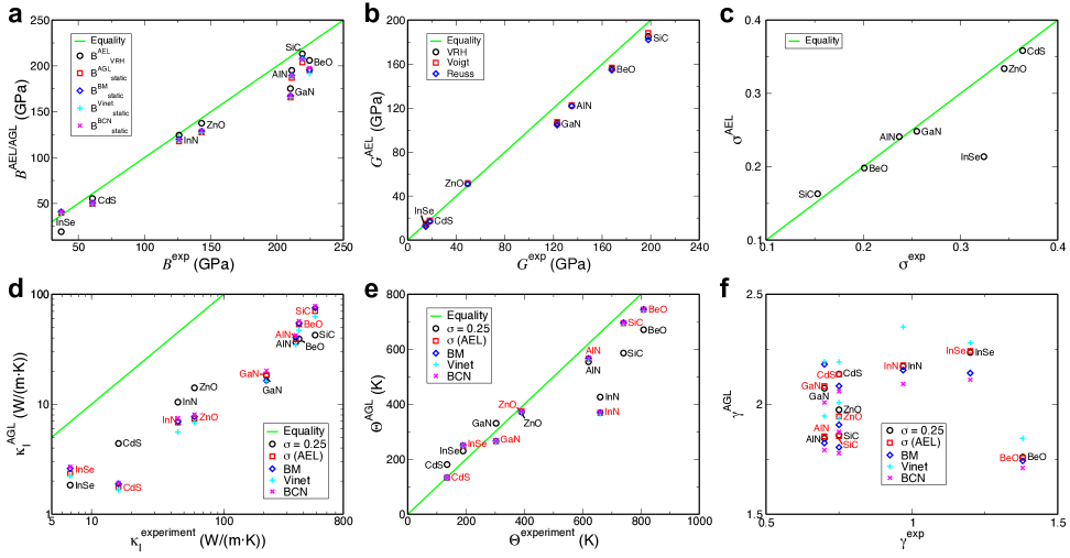
Figure 3: (a) Bulk modulus, (b) shear modulus, (c) Poisson ratio, (d) lattice thermal conductivity, (e) Debye temperature and (f) Grüneisen parameter of hexagonal structure semiconductors. The Debye temperatures plotted in (e) are $\theta_{\mathrm{a}}$, except for InSe and InN where $\theta_{\mathrm{D}}$ values are quoted in Refs. Snyder_jmatchem_2011, ; Ioffe_Inst_DB, ; Krukowski_jphyschemsolids_1998, .

For the shear modulus, the experimental values $G^{\mathrm{exp}}$ are compared to the AEL values $G_{\begin{subarray}{c}\scalebox{0.6}{Voigt}\end{subarray}}^{\begin{subarray}{c}\scalebox{0.6}{AEL}\end{subarray}}$, $G_{\begin{subarray}{c}\scalebox{0.6}{Reuss}\end{subarray}}^{\begin{subarray}{c}\scalebox{0.6}{AEL}\end{subarray}}$ and $G_{\begin{subarray}{c}\scalebox{0.6}{VRH}\end{subarray}}^{\begin{subarray}{c}\scalebox{0.6}{AEL}\end{subarray}}$. As can be seen in Table 7 and Fig. 3(b), the agreement with the experimental values is very good. Similarly good agreement is obtained for the Poisson ratio of most materials (Table 7 and Fig. 3(c)), with a single exception for InSe where the calculation deviates significantly from the experiment. The Pearson (i.e. linear, Eq. (40)) and Spearman (i.e. rank order, Eq. (41)) correlations between the calculated elastic properties and their experimental values are generally quite high (Table 9), ranging from 0.851 and 0.893 respectively for $\sigma^{\mathrm{exp}}$ vs. $\sigma^{\begin{subarray}{c}\scalebox{0.6}{AEL}\end{subarray}}$, up to 0.998 and 1.0 for $G^{\mathrm{exp}}$ vs. $G_{\begin{subarray}{c}\scalebox{0.6}{VRH}\end{subarray}}^{\begin{subarray}{c}\scalebox{0.6}{AEL}\end{subarray}}$.

The Materials Project values of $B_{\begin{subarray}{c}\scalebox{0.6}{VRH}\end{subarray}}^{\begin{subarray}{c}\scalebox{0.6}{MP}\end{subarray}}$, $G_{\begin{subarray}{c}\scalebox{0.6}{VRH}\end{subarray}}^{\begin{subarray}{c}\scalebox{0.6}{MP}\end{subarray}}$ and $\sigma^{\begin{subarray}{c}\scalebox{0.6}{MP}\end{subarray}}$ for hexagonal structure materials are also shown in Table 7, where available. The Pearson correlations values for the experimental results with the available values of $B_{\begin{subarray}{c}\scalebox{0.6}{VRH}\end{subarray}}^{\begin{subarray}{c}\scalebox{0.6}{MP}\end{subarray}}$, $G_{\begin{subarray}{c}\scalebox{0.6}{VRH}\end{subarray}}^{\begin{subarray}{c}\scalebox{0.6}{MP}\end{subarray}}$ and $\sigma^{\begin{subarray}{c}\scalebox{0.6}{MP}\end{subarray}}$ were calculated to be 0.984, 0.998 and 0.993, respectively, while the respective Spearman correlations were 0.943, 1.0 and 0.943, and the RMSrD values were 0.117, 0.116 and 0.034. For comparison, the corresponding Pearson correlations for the same subset of materials for $B_{\begin{subarray}{c}\scalebox{0.6}{VRH}\end{subarray}}^{\begin{subarray}{c}\scalebox{0.6}{AEL}\end{subarray}}$, $G_{\begin{subarray}{c}\scalebox{0.6}{VRH}\end{subarray}}^{\begin{subarray}{c}\scalebox{0.6}{AEL}\end{subarray}}$ and $\sigma^{\begin{subarray}{c}\scalebox{0.6}{AEL}\end{subarray}}$ are 0.986, 0.998, and 0.998 respectively, while the respective Spearman correlations were 0.943, 1.0 and 1.0, and the RMSrD values were 0.100, 0.091 and 0.036. These correlation values are very similar, and the general close agreement for the results for the values of $B_{\begin{subarray}{c}\scalebox{0.6}{VRH}\end{subarray}}^{\begin{subarray}{c}\scalebox{0.6}{AEL}\end{subarray}}$, $G_{\begin{subarray}{c}\scalebox{0.6}{VRH}\end{subarray}}^{\begin{subarray}{c}\scalebox{0.6}{AEL}\end{subarray}}$ and $\sigma^{\begin{subarray}{c}\scalebox{0.6}{AEL}\end{subarray}}$ with those of $B_{\begin{subarray}{c}\scalebox{0.6}{VRH}\end{subarray}}^{\begin{subarray}{c}\scalebox{0.6}{MP}\end{subarray}}$, $G_{\begin{subarray}{c}\scalebox{0.6}{VRH}\end{subarray}}^{\begin{subarray}{c}\scalebox{0.6}{MP}\end{subarray}}$ and $\sigma^{\begin{subarray}{c}\scalebox{0.6}{MP}\end{subarray}}$ demonstrate that the small differences in the parameters used for the DFT calculations make little difference to the results, indicating that the parameter set used here is robust for high-throughput calculations.

The thermal properties calculated using AGL are compared to the experimental values in Table 8 and are also plotted in Fig. 3. For the Debye temperature, the $\theta^{\mathrm{exp}}$ values taken from Ref. Morelli_Slack_2006, are for $\theta_{\mathrm{a}}$, and are mostly in good agreement with the calculated $\theta_{\mathrm{a}}^{\begin{subarray}{c}\scalebox{0.6}{AGL}\end{subarray}}$ values. As in the case of the other materials sets, the values obtained using the numerical $E(V)$ fit and the three different equations of state are very similar to each other, whereas $\theta_{\begin{subarray}{c}\scalebox{0.6}{D}\end{subarray}}^{\begin{subarray}{c}\scalebox{0.6}{AGL}\end{subarray}}$ calculated using $\sigma=0.25$ differs significantly. In fact, the values of $\theta_{\begin{subarray}{c}\scalebox{0.6}{D}\end{subarray}}^{\begin{subarray}{c}\scalebox{0.6}{AGL}\end{subarray}}$ calculated with $\sigma^{\begin{subarray}{c}\scalebox{0.6}{AEL}\end{subarray}}$ have a lower the correlation with $\theta^{\mathrm{exp}}$ than the values calculated with $\sigma=0.25$ do, although the RMSrD values are lower when $\sigma^{\begin{subarray}{c}\scalebox{0.6}{AEL}\end{subarray}}$ is used. However, most of this discrepancy appears to be due to the clear outlier value for the material InN. When the values for this material are removed from the data set, the Pearson correlation values become very similar when both the $\sigma=0.25$ and $\sigma=\sigma^{\begin{subarray}{c}\scalebox{0.6}{AEL}\end{subarray}}$ values are used, increasing to 0.995 and 0.994 respectively.

Table 8: Lattice thermal conductivity, Debye temperature and Grüneisen parameter of hexagonal structure semiconductors, comparing the effect of using the calculated value of the Poisson ratio to previous approximation of $\sigma=0.25$. The values listed for $\theta^{\mathrm{exp}}$ are $\theta_{\mathrm{a}}$, except 190K for InSe Snyder_jmatchem_2011 and 660K for InN Ioffe_Inst_DB ; Krukowski_jphyschemsolids_1998 which are $\theta_{\mathrm{D}}$. “N/A” = Not available for that source. Units: $\kappa$ in (W/(m$\cdot$K)), $\theta$ in (K).

Comp.	$\kappa^{\mathrm{exp}}$	$\kappa^{\begin{subarray}{c}\scalebox{0.6}{AGL}\end{subarray}}$	$\kappa^{\begin{subarray}{c}\scalebox{0.6}{AGL}\end{subarray}}$	$\theta^{\mathrm{exp}}$	$\theta_{\begin{subarray}{c}\scalebox{0.6}{D}\end{subarray}}^{\begin{subarray}{c}\scalebox{0.6}{AGL}\end{subarray}}$	$\theta_{\begin{subarray}{c}\scalebox{0.6}{D}\end{subarray}}^{\begin{subarray}{c}\scalebox{0.6}{AGL}\end{subarray}}$	$\theta_{\begin{subarray}{c}\scalebox{0.6}{D}\end{subarray}}^{\begin{subarray}{c}\scalebox{0.6}{AEL}\end{subarray}}$	$\gamma^{\mathrm{exp}}$	$\gamma^{\begin{subarray}{c}\scalebox{0.6}{AGL}\end{subarray}}$	$\gamma^{\begin{subarray}{c}\scalebox{0.6}{AGL}\end{subarray}}$
					($\theta_{\mathrm{a}}^{\begin{subarray}{c}\scalebox{0.6}{AGL}\end{subarray}}$)	($\theta_{\mathrm{a}}^{\begin{subarray}{c}\scalebox{0.6}{AGL}\end{subarray}}$)
		($\sigma=0.25$) curtarolo:art96			($\sigma=0.25$) curtarolo:art96				($\sigma=0.25$) curtarolo:art96
SiC	490 Morelli_Slack_2006	42.49	70.36	740 Morelli_Slack_2006	930	1103	1138	0.75 Morelli_Slack_2006	1.86	1.86
					(586)	(695)
AlN	350 Morelli_Slack_2006	36.73	39.0	620 Morelli_Slack_2006	880	898	917	0.7 Morelli_Slack_2006	1.85	1.85
					(554)	(566)
GaN	210 Morelli_Slack_2006	18.17	18.54	390 Morelli_Slack_2006	592	595	606	0.7 Morelli_Slack_2006	2.07	2.08
					(373)	(375)
ZnO	60 Morelli_Slack_2006	14.10	7.39	303 Morelli_Slack_2006	525	422	427	0.75 Morelli_Slack_2006	1.97	1.94
					(331)	(266)
BeO	370 Morelli_Slack_2006	39.26	53.36	809 Morelli_Slack_2006	1065	1181	1235	1.38 Slack_JAP_1975 ; Cline_JAP_1967 ; Morelli_Slack_2006	1.76	1.76
					(671)	(744)
CdS	16 Morelli_Slack_2006	4.40	1.76	135 Morelli_Slack_2006	287	211	213	0.75 Morelli_Slack_2006	2.14	2.14
					(181)	(133)
InSe	6.9 Snyder_jmatchem_2011	1.84	2.34	190 Snyder_jmatchem_2011	230	249	168	1.2 Snyder_jmatchem_2011	2.24	2.24
					(115)	(125)
InN	45 Ioffe_Inst_DB ; Krukowski_jphyschemsolids_1998	10.44	6.82	660 Ioffe_Inst_DB ; Krukowski_jphyschemsolids_1998	426	369	370	0.97 Krukowski_jphyschemsolids_1998	2.17	2.18
					(268)	(232)

The experimental and calculated values of the Grüneisen parameter are listed in Table 8 and in the supplementary information, and are plotted in Fig. 3(f). Again, the Debye model does not reproduce the experimental data, as the calculated values are often 2 to 3 times too large and the RMSrD is larger than 1.5. The corresponding correlation, shown in Table 9, are also quite poor, with no value higher than 0.160 for the Spearman correlations, and negative values for the Pearson correlations.

The comparison between the experimental thermal conductivity $\kappa^{\mathrm{exp}}$ and the calculated values is also quite poor (Fig. 3(d) and Table 8), with RMSrD values of the order of 0.9. Considerable disagreements also exist between different experimental reports for most materials. Nevertheless, the Pearson correlations between the AGL calculated thermal conductivity values and the experimental values are high, ranging from $0.974$ to $0.980$, while the Spearman correlations are even higher, ranging from $0.976$ to $1.0$.

Table 9: Correlations between experimental values and AEL and AGL results for elastic and thermal properties for hexagonal structure semiconductors.

Property	Pearson	Spearman	RMSrD
	(Linear)	(Rank Order)
$\kappa^{\mathrm{exp}}$ vs. $\kappa^{\begin{subarray}{c}\scalebox{0.6}{AGL}\end{subarray}}$ ($\sigma=0.25$) curtarolo:art96	0.977	1.0	0.887
$\kappa^{\mathrm{exp}}$ vs. $\kappa^{\begin{subarray}{c}\scalebox{0.6}{AGL}\end{subarray}}$	0.980	0.976	0.911
$\kappa^{\mathrm{exp}}$ vs. $\kappa^{\begin{subarray}{c}\scalebox{0.6}{BM}\end{subarray}}$	0.974	0.976	0.904
$\kappa^{\mathrm{exp}}$ vs. $\kappa^{\begin{subarray}{c}\scalebox{0.6}{Vinet}\end{subarray}}$	0.980	0.976	0.926
$\kappa^{\mathrm{exp}}$ vs. $\kappa^{\begin{subarray}{c}\scalebox{0.6}{BCN}\end{subarray}}$	0.980	0.976	0.895
$\theta_{\mathrm{a}}^{\mathrm{exp}}$ vs. $\theta_{\mathrm{a}}^{\begin{subarray}{c}\scalebox{0.6}{AGL}\end{subarray}}$ ($\sigma=0.25$) curtarolo:art96	0.960	0.976	0.233
$\theta_{\mathrm{a}}^{\mathrm{exp}}$ vs. $\theta_{\mathrm{a}}^{\begin{subarray}{c}\scalebox{0.6}{AGL}\end{subarray}}$	0.921	0.929	0.216
$\theta_{\mathrm{a}}^{\mathrm{exp}}$ vs. $\theta_{\mathrm{a}}^{\begin{subarray}{c}\scalebox{0.6}{BM}\end{subarray}}$	0.921	0.929	0.217
$\theta_{\mathrm{a}}{\mathrm{exp}}$ vs. $\theta_{\mathrm{a}}^{\begin{subarray}{c}\scalebox{0.6}{Vinet}\end{subarray}}$	0.920	0.929	0.218
$\theta_{\mathrm{a}}^{\mathrm{exp}}$ vs. $\theta_{\mathrm{a}}^{\begin{subarray}{c}\scalebox{0.6}{BCN}\end{subarray}}$	0.921	0.929	0.216
$\gamma^{\mathrm{exp}}$ vs. $\gamma^{\begin{subarray}{c}\scalebox{0.6}{AGL}\end{subarray}}$ ($\sigma=0.25$) curtarolo:art96	-0.039	0.160	1.566
$\gamma^{\mathrm{exp}}$ vs. $\gamma^{\begin{subarray}{c}\scalebox{0.6}{AGL}\end{subarray}}$	-0.029	0.160	1.563
$\gamma^{\mathrm{exp}}$ vs. $\gamma^{\begin{subarray}{c}\scalebox{0.6}{BM}\end{subarray}}$	-0.124	-0.233	1.547
$\gamma^{\mathrm{exp}}$ vs. $\gamma^{\begin{subarray}{c}\scalebox{0.6}{Vinet}\end{subarray}}$	-0.043	0.012	1.677
$\gamma^{\mathrm{exp}}$ vs. $\gamma^{\begin{subarray}{c}\scalebox{0.6}{BCN}\end{subarray}}$	-0.054	0.098	1.467
$B^{\mathrm{exp}}$ vs. $B_{\begin{subarray}{c}\scalebox{0.6}{VRH}\end{subarray}}^{\begin{subarray}{c}\scalebox{0.6}{AEL}\end{subarray}}$	0.990	0.976	0.201
$B^{\mathrm{exp}}$ vs. $B_{\begin{subarray}{c}\scalebox{0.6}{Static}\end{subarray}}^{\begin{subarray}{c}\scalebox{0.6}{AGL}\end{subarray}}$	0.990	0.976	0.138
$B^{\mathrm{exp}}$ vs. $B_{\begin{subarray}{c}\scalebox{0.6}{Static}\end{subarray}}^{\begin{subarray}{c}\scalebox{0.6}{BM}\end{subarray}}$	0.988	0.976	0.133
$B^{\mathrm{exp}}$ vs. $B_{\begin{subarray}{c}\scalebox{0.6}{Static}\end{subarray}}^{\begin{subarray}{c}\scalebox{0.6}{Vinet}\end{subarray}}$	0.988	0.976	0.139
$B^{\mathrm{exp}}$ vs. $B_{\begin{subarray}{c}\scalebox{0.6}{Static}\end{subarray}}^{\begin{subarray}{c}\scalebox{0.6}{BCN}\end{subarray}}$	0.990	0.976	0.130
$G^{\mathrm{exp}}$ vs. $G_{\begin{subarray}{c}\scalebox{0.6}{VRH}\end{subarray}}^{\begin{subarray}{c}\scalebox{0.6}{AEL}\end{subarray}}$	0.998	1.0	0.090
$G^{\mathrm{exp}}$ vs. $G_{\begin{subarray}{c}\scalebox{0.6}{Voigt}\end{subarray}}^{\begin{subarray}{c}\scalebox{0.6}{AEL}\end{subarray}}$	0.998	1.0	0.076
$G^{\mathrm{exp}}$ vs. $G_{\begin{subarray}{c}\scalebox{0.6}{Reuss}\end{subarray}}^{\begin{subarray}{c}\scalebox{0.6}{AEL}\end{subarray}}$	0.998	1.0	0.115
$\sigma^{\mathrm{exp}}$ vs. $\sigma^{\begin{subarray}{c}\scalebox{0.6}{AEL}\end{subarray}}$	0.851	0.893	0.143

As for the rocksalt and zincblende material sets, Ref. Morelli_Slack_2006, (Table 2.3) includes values of the thermal conductivity at 300K for wurzite structure materials, calculated using the experimental values of the Debye temperature and Grüneisen parameter in the Leibfried-Schlömann equation. The Pearson and Spearman correlations are $0.996$ and $1.0$ respectively, which are slightly higher than the correlations obtained using the AGL calculated quantities. The difference is insignificant since all of these correlations are very high and could reliably serve as a screening tool of the thermal conductivity. However, as we noted in our previous work on AGL curtarolo:art96 , the high correlations calculated with the experimental $\theta_{\mathrm{a}}$ and $\gamma$ were obtained using $\gamma=0.75$ for BeO. Table 2.3 of Ref. Morelli_Slack_2006, also cites an alternative value of $\gamma=1.38$ for BeO (Table 8). Using this outlier value would severely degrade the results down to $0.7$, for the Pearson correlation, and $0.829$, for the Spearman correlation. These values are too low for a reliable screening tool. This demonstrates the ability of the AEL-AGL calculations to compensate for anomalies in the experimental data when they exist and still provide a reliable screening method for the thermal conductivity.

III.4 Rhombohedral materials

The elastic properties of a few materials with rhombohedral structures (spacegroups: R$\overline{3}$mR, $\#$166, R$\overline{3}$mH, $\#$166; Pearson symbol: hR5; AFLOW prototype: A2B3_hR5_166_c_ac curtarolo:art121 ; and spacegroup: R$\overline{3}$cH, $\#$167; Pearson symbol: hR10; AFLOW prototype: A2B3_hR10_167_c_e curtarolo:art121 ) are shown in Table 10 (we have left out the material Fe₂O₃ which was included in the data set in Table IV of Ref. curtarolo:art96, , due to convergence issues with some of the strained structures required for the calculation of the elastic tensor). The comparison between experiment and calculation is qualitatively reasonable, but the scarcity of experimental results does not allow for a proper correlation analysis.

Table 10: Bulk modulus, shear modulus and Poisson ratio of rhombohedral semiconductors. “N/A” = Not available for that source. Units: $B$ and $G$ in (GPa).

Comp.	$B^{\mathrm{exp}}$	$B_{\begin{subarray}{c}\scalebox{0.6}{VRH}\end{subarray}}^{\begin{subarray}{c}\scalebox{0.6}{AEL}\end{subarray}}$	$B_{\begin{subarray}{c}\scalebox{0.6}{VRH}\end{subarray}}^{\begin{subarray}{c}\scalebox{0.6}{MP}\end{subarray}}$	$B_{\begin{subarray}{c}\scalebox{0.6}{Static}\end{subarray}}^{\begin{subarray}{c}\scalebox{0.6}{AGL}\end{subarray}}$	$B_{\begin{subarray}{c}\scalebox{0.6}{Static}\end{subarray}}^{\begin{subarray}{c}\scalebox{0.6}{BM}\end{subarray}}$	$B_{\begin{subarray}{c}\scalebox{0.6}{Static}\end{subarray}}^{\begin{subarray}{c}\scalebox{0.6}{Vinet}\end{subarray}}$	$B_{\begin{subarray}{c}\scalebox{0.6}{Static}\end{subarray}}^{\begin{subarray}{c}\scalebox{0.6}{BCN}\end{subarray}}$	$G^{\mathrm{exp}}$	$G_{\begin{subarray}{c}\scalebox{0.6}{Voigt}\end{subarray}}^{\begin{subarray}{c}\scalebox{0.6}{AEL}\end{subarray}}$	$G_{\begin{subarray}{c}\scalebox{0.6}{Reuss}\end{subarray}}^{\begin{subarray}{c}\scalebox{0.6}{AEL}\end{subarray}}$	$G_{\begin{subarray}{c}\scalebox{0.6}{VRH}\end{subarray}}^{\begin{subarray}{c}\scalebox{0.6}{AEL}\end{subarray}}$	$G_{\begin{subarray}{c}\scalebox{0.6}{VRH}\end{subarray}}^{\begin{subarray}{c}\scalebox{0.6}{MP}\end{subarray}}$	$\sigma^{\mathrm{exp}}$	$\sigma^{\begin{subarray}{c}\scalebox{0.6}{AEL}\end{subarray}}$	$\sigma^{\begin{subarray}{c}\scalebox{0.6}{MP}\end{subarray}}$
Bi2Te3	37.0 Semiconductors_BasicData_Springer ; Jenkins_ElasticBi2Te3_PRB_1972	28.8	15.0	43.7	44.4	43.3	44.5	22.4 Semiconductors_BasicData_Springer ; Jenkins_ElasticBi2Te3_PRB_1972	23.5	16.3	19.9	10.9	0.248 Semiconductors_BasicData_Springer ; Jenkins_ElasticBi2Te3_PRB_1972	0.219	0.21
Sb2Te3	N/A	22.9	N/A	45.3	46.0	45.2	46.0	N/A	20.6	14.5	17.6	N/A	N/A	0.195	N/A
Al2O3	254 Goto_ElasticAl2O3_JGPR_1989	231	232	222	225	224	224	163.1 Goto_ElasticAl2O3_JGPR_1989	149	144	147	147	0.235 Goto_ElasticAl2O3_JGPR_1989	0.238	0.24
Cr2O3	234 Alberts_ElasticCr2O3_JMMM_1976	203	203	198	202	201	201	129 Alberts_ElasticCr2O3_JMMM_1976	115	112	113	113	0.266 Alberts_ElasticCr2O3_JMMM_1976	0.265	0.27
Bi2Se3	N/A	93.9	N/A	57.0	57.5	56.4	57.9	N/A	53.7	28.0	40.9	N/A	N/A	0.310	N/A

The thermal properties calculated using AGL are compared to the experimental values in Table 11 and the thermal conductivity is also plotted in Fig. 4(a). The experimental Debye temperatures are $\theta_{\begin{subarray}{c}\scalebox{0.6}{D}\end{subarray}}$ for Bi₂Te₃ and Sb₂Te₃, and $\theta_{\mathrm{a}}$ for Al₂O₃. The values obtained using the numerical $E(V)$ fit and the three different equations of state (see supplementary material) are very similar, but just roughly reproduce the experiments.

Table 11: Lattice thermal conductivity, Debye temperatures and Grüneisen parameter of rhombohedral semiconductors, comparing the effect of using the calculated value of the Poisson ratio to previous approximation of $\sigma=0.25$. The experimental Debye temperatures are $\theta_{\mathrm{D}}$ for Bi₂Te₃ and Sb₂Te₃, and $\theta_{\mathrm{a}}$ for Al₂O₃. “N/A” = Not available for that source. Units: $\kappa$ in (W/(m$\cdot$K)), $\theta$ in (K).

Comp.	$\kappa^{\mathrm{exp}}$	$\kappa^{\begin{subarray}{c}\scalebox{0.6}{AGL}\end{subarray}}$	$\kappa^{\begin{subarray}{c}\scalebox{0.6}{AGL}\end{subarray}}$	$\theta^{\mathrm{exp}}$	$\theta_{\begin{subarray}{c}\scalebox{0.6}{D}\end{subarray}}^{\begin{subarray}{c}\scalebox{0.6}{AGL}\end{subarray}}$	$\theta_{\begin{subarray}{c}\scalebox{0.6}{D}\end{subarray}}^{\begin{subarray}{c}\scalebox{0.6}{AGL}\end{subarray}}$	$\theta_{\begin{subarray}{c}\scalebox{0.6}{D}\end{subarray}}^{\begin{subarray}{c}\scalebox{0.6}{AEL}\end{subarray}}$	$\gamma^{\mathrm{exp}}$	$\gamma^{\begin{subarray}{c}\scalebox{0.6}{AGL}\end{subarray}}$	$\gamma^{\begin{subarray}{c}\scalebox{0.6}{AGL}\end{subarray}}$
					($\theta_{\mathrm{a}}^{\begin{subarray}{c}\scalebox{0.6}{AGL}\end{subarray}}$)	($\theta_{\mathrm{a}}^{\begin{subarray}{c}\scalebox{0.6}{AGL}\end{subarray}}$)
		($\sigma=0.25$) curtarolo:art96			($\sigma=0.25$) curtarolo:art96				($\sigma=0.25$) curtarolo:art96
Bi2Te3	1.6 Snyder_jmatchem_2011	2.79	3.35	155 Snyder_jmatchem_2011	191	204	161	1.49 Snyder_jmatchem_2011	2.13	2.14
					(112)	(119)
Sb2Te3	2.4 Snyder_jmatchem_2011	2.90	4.46	160 Snyder_jmatchem_2011	217	243	170	1.49 Snyder_jmatchem_2011	2.2	2.11
					(127)	(142)
Al2O3	30 Slack_PR_1962	20.21	21.92	390 slack	927	952	975	1.32 slack	1.91	1.91
					(430)	(442)
Cr2O3	16 Landolt-Bornstein ; Bruce_PRB_1977	10.87	12.03	N/A	733	717	720	N/A	2.26	2.10
					(340)	(333)
Bi2Se3	1.34 Landolt-Bornstein	3.60	2.41	N/A	223	199	241	N/A	2.08	2.12
					(130)	(116)

The calculated Grüneisen parameters are about 50% larger than the experimental ones, and the value of $\sigma$ used makes a little difference in the calculation. The absolute agreement between the AGL values and $\kappa^{\mathrm{exp}}$ is also quite poor (Fig. 4(a)). However, despite all these discrepancies, the Pearson correlations between the calculated thermal conductivities and the experimental values are all high, of the order of $0.998$, while the Spearman correlations range from $0.7$ to $1.0$, with all of the different equations of state having very similar correlations with experiment. Using the calculated $\sigma^{\begin{subarray}{c}\scalebox{0.6}{AEL}\end{subarray}}$, vs. the rough Cauchy approximation, improves the Spearman correlation from $0.7$ to $1.0$.

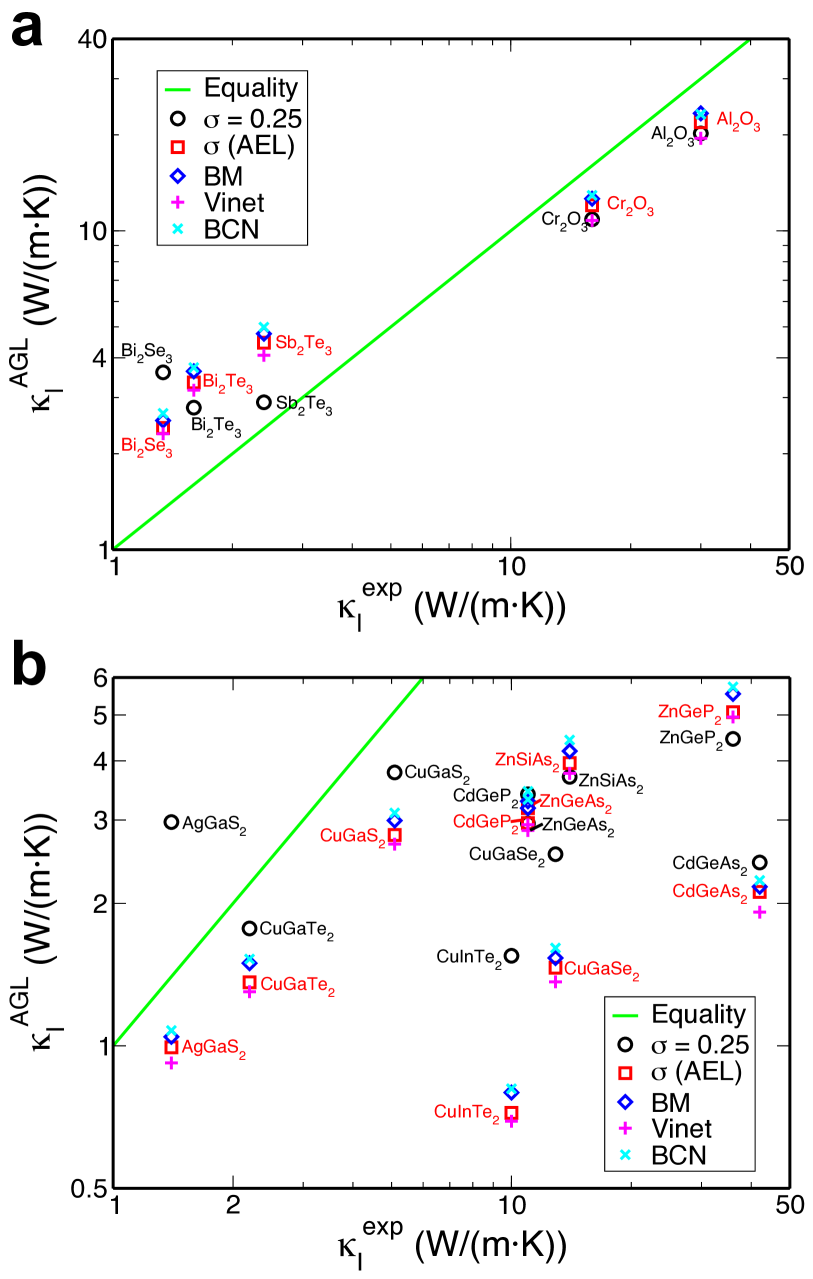
Figure 4: (a) Lattice thermal conductivity of rhombohedral semiconductors at 300K. (b) Lattice thermal conductivity of body-centred tetragonal semiconductors at 300K.

Table 12: Correlations between experimental values and AEL and AGL results for elastic and thermal properties for rhombohedral structure semiconductors.

Property	Pearson	Spearman	RMSrD
	(Linear)	(Rank Order)
$\kappa^{\mathrm{exp}}$ vs. $\kappa^{\begin{subarray}{c}\scalebox{0.6}{AGL}\end{subarray}}$ ($\sigma=0.25$) curtarolo:art96	0.997	0.7	0.955
$\kappa^{\mathrm{exp}}$ vs. $\kappa^{\begin{subarray}{c}\scalebox{0.6}{AGL}\end{subarray}}$	0.998	1.0	0.821
$\kappa^{\mathrm{exp}}$ vs. $\kappa^{\begin{subarray}{c}\scalebox{0.6}{BM}\end{subarray}}$	0.997	1.0	0.931
$\kappa^{\mathrm{exp}}$ vs. $\kappa^{\begin{subarray}{c}\scalebox{0.6}{Vinet}\end{subarray}}$	0.998	1.0	0.741
$\kappa^{\mathrm{exp}}$ vs. $\kappa^{\begin{subarray}{c}\scalebox{0.6}{BCN}\end{subarray}}$	0.997	1.0	1.002

III.5 Body-centred tetragonal materials

The mechanical properties of the body-centred tetragonal materials (spacegroup: I$\overline{4}2$d, $\#$122; Pearson symbol: tI16; AFLOW prototype: ABC2_tI16_122_a_b_d curtarolo:art121 ) of Table V of Ref. curtarolo:art96, are reported in Table 13. The calculated bulk moduli miss considerably the few available experimental results, while the shear moduli are well reproduced. Reasonable estimates are also obtained for the Poisson ratio.

Table 13: Bulk modulus, shear modulus and Poisson ratio of body-centred tetragonal semiconductors. Note that there appears to be an error in Table 1 of Ref. Fernandez_ElasticCuInTe_PSSa_1990, where the bulk modulus values are stated to be in units of $10^{12}$ Pa. This seems unlikely, as that would give a bulk modulus for CuInTe₂ an order of magnitude larger than that for diamond. Also, units of $10^{12}$ Pa would be inconsistent with the experimental results listed in Ref. Neumann_ElasticCuInTe_PSSa_1986, , so therefore it seems that these values are in units of $10^{10}$ Pa, which are the values shown here. “N/A” = Not available for that source. Units: $B$ and $G$ in (GPa).

Comp.	$B^{\mathrm{exp}}$	$B_{\begin{subarray}{c}\scalebox{0.6}{VRH}\end{subarray}}^{\begin{subarray}{c}\scalebox{0.6}{AEL}\end{subarray}}$	$B_{\begin{subarray}{c}\scalebox{0.6}{VRH}\end{subarray}}^{\begin{subarray}{c}\scalebox{0.6}{MP}\end{subarray}}$	$B_{\begin{subarray}{c}\scalebox{0.6}{Static}\end{subarray}}^{\begin{subarray}{c}\scalebox{0.6}{AGL}\end{subarray}}$	$B_{\begin{subarray}{c}\scalebox{0.6}{Static}\end{subarray}}^{\begin{subarray}{c}\scalebox{0.6}{BM}\end{subarray}}$	$B_{\begin{subarray}{c}\scalebox{0.6}{Static}\end{subarray}}^{\begin{subarray}{c}\scalebox{0.6}{Vinet}\end{subarray}}$	$B_{\begin{subarray}{c}\scalebox{0.6}{Static}\end{subarray}}^{\begin{subarray}{c}\scalebox{0.6}{BCN}\end{subarray}}$	$G^{\mathrm{exp}}$	$G_{\begin{subarray}{c}\scalebox{0.6}{Voigt}\end{subarray}}^{\begin{subarray}{c}\scalebox{0.6}{AEL}\end{subarray}}$	$G_{\begin{subarray}{c}\scalebox{0.6}{Reuss}\end{subarray}}^{\begin{subarray}{c}\scalebox{0.6}{AEL}\end{subarray}}$	$G_{\begin{subarray}{c}\scalebox{0.6}{VRH}\end{subarray}}^{\begin{subarray}{c}\scalebox{0.6}{AEL}\end{subarray}}$	$G_{\begin{subarray}{c}\scalebox{0.6}{VRH}\end{subarray}}^{\begin{subarray}{c}\scalebox{0.6}{MP}\end{subarray}}$	$\sigma^{\mathrm{exp}}$	$\sigma^{\begin{subarray}{c}\scalebox{0.6}{AEL}\end{subarray}}$	$\sigma^{\begin{subarray}{c}\scalebox{0.6}{MP}\end{subarray}}$
CuGaTe2	N/A	47.0	N/A	42.5	43.2	42.0	43.5	N/A	25.1	22.1	23.6	N/A	N/A	0.285	N/A
ZnGeP2	N/A	73.1	74.9	70.1	71.1	70.0	71.4	N/A	50.5	46.2	48.4	48.9	N/A	0.229	0.23
ZnSiAs2	N/A	67.4	65.9	63.4	64.3	63.1	64.6	N/A	44.4	40.4	42.4	42.2	N/A	0.240	0.24
CuInTe2	36.0 Neumann_ElasticCuInTe_PSSa_1986	53.9	N/A	38.6	39.2	38.2	39.4	N/A	20.4	17.2	18.8	N/A	0.313 Fernandez_ElasticCuInTe_PSSa_1990	0.344	N/A
	45.4 Fernandez_ElasticCuInTe_PSSa_1990
AgGaS2	67.0 Grimsditch_ElasticAgGaS2_PRB_1975	70.3	N/A	56.2	57.1	56.0	57.4	20.8 Grimsditch_ElasticAgGaS2_PRB_1975	20.7	17.4	19.1	N/A	0.359 Grimsditch_ElasticAgGaS2_PRB_1975	0.375	N/A
CdGeP2	N/A	65.3	65.2	60.7	61.6	60.4	61.9	N/A	37.7	33.3	35.5	35.0	N/A	0.270	0.27
CdGeAs2	69.9 Hailing_ElasticCdGeAs_JPCSS_1982	52.6	N/A	49.2	49.6	48.3	49.9	29.5 Hailing_ElasticCdGeAs_JPCSS_1982	30.9	26.2	28.6	N/A	0.315 Hailing_ElasticCdGeAs_JPCSS_1982	0.270	N/A
CuGaS2	94.0 Bettini_ElasticCuGaS_SSC_1975	73.3	N/A	69.0	69.9	68.7	70.6	N/A	37.8	32.4	35.1	N/A	N/A	0.293	N/A
CuGaSe2	N/A	69.9	N/A	54.9	55.6	54.4	56.0	N/A	30.3	26.0	28.1	N/A	N/A	0.322	N/A
ZnGeAs2	N/A	59.0	N/A	56.2	56.7	55.5	57.1	N/A	39.0	35.6	37.3	N/A	N/A	0.239	N/A

The thermal properties are reported in Table 14 and Fig. 4(b). The $\theta^{\mathrm{exp}}$ values are all for $\theta_{\begin{subarray}{c}\scalebox{0.6}{D}\end{subarray}}$, and in most cases are in good agreement with the values obtained with the AEL calculated $\sigma$. The values from the numerical $E(V)$ fit and the three different equations of state are again very similar, but differ significantly from $\theta_{\begin{subarray}{c}\scalebox{0.6}{D}\end{subarray}}^{\begin{subarray}{c}\scalebox{0.6}{AGL}\end{subarray}}$ calculated with $\sigma=0.25$.

Table 14: Lattice thermal conductivity at 300K, Debye temperatures and Grüneisen parameter of body-centred tetragonal semiconductors, comparing the effect of using the calculated value of the Poisson ratio to previous approximation of $\sigma=0.25$. “N/A” = Not available for that source. Units: $\kappa$ in (W/(m$\cdot$K)), $\theta$ in (K).

Comp.	$\kappa^{\mathrm{exp}}$	$\kappa^{\begin{subarray}{c}\scalebox{0.6}{AGL}\end{subarray}}$	$\kappa^{\begin{subarray}{c}\scalebox{0.6}{AGL}\end{subarray}}$	$\theta^{\mathrm{exp}}$	$\theta_{\begin{subarray}{c}\scalebox{0.6}{D}\end{subarray}}^{\begin{subarray}{c}\scalebox{0.6}{AGL}\end{subarray}}$	$\theta_{\begin{subarray}{c}\scalebox{0.6}{D}\end{subarray}}^{\begin{subarray}{c}\scalebox{0.6}{AGL}\end{subarray}}$	$\theta_{\begin{subarray}{c}\scalebox{0.6}{D}\end{subarray}}^{\begin{subarray}{c}\scalebox{0.6}{AEL}\end{subarray}}$	$\gamma^{\mathrm{exp}}$	$\gamma^{\begin{subarray}{c}\scalebox{0.6}{AGL}\end{subarray}}$	$\gamma^{\begin{subarray}{c}\scalebox{0.6}{AGL}\end{subarray}}$
					($\theta_{\mathrm{a}}^{\begin{subarray}{c}\scalebox{0.6}{AGL}\end{subarray}}$)	($\theta_{\mathrm{a}}^{\begin{subarray}{c}\scalebox{0.6}{AGL}\end{subarray}}$)
		($\sigma=0.25$) curtarolo:art96			($\sigma=0.25$) curtarolo:art96				($\sigma=0.25$) curtarolo:art96
CuGaTe2	2.2 Snyder_jmatchem_2011	1.77	1.36	226 Snyder_jmatchem_2011	234	215	218	1.46 Snyder_jmatchem_2011	2.32	2.32
					(117)	(108)
ZnGeP2	35 Landolt-Bornstein ; Beasley_AO_1994	4.45	5.07	500 Landolt-Bornstein	390	408	411	N/A	2.13	2.14
	36 Landolt-Bornstein ; Beasley_AO_1994			428 Abrahams_JCP_1975	(195)	(204)
	18 Landolt-Bornstein ; Shay_1975 ; Masumoto_JPCS_1966
ZnSiAs2	14Landolt-Bornstein ; Shay_1975 ; Masumoto_JPCS_1966	3.70	3.96	347 Landolt-Bornstein ; Bohnhammel_PSSa_1981	342	350	354	N/A	2.15	2.15
					(171)	(175)
CuInTe2	10Landolt-Bornstein ; Rincon_PSSa_1995	1.55	0.722	185 Landolt-Bornstein ; Rincon_PSSa_1995	215	166	185	0.93 Rincon_PSSa_1995	2.33	2.32
				195 Landolt-Bornstein ; Bohnhammel_PSSa_1982	(108)	(83)
AgGaS2	1.4Landolt-Bornstein ; Beasley_AO_1994	2.97	0.993	255 Landolt-Bornstein ; Abrahams_JCP_1975	324	224	237	N/A	2.20	2.20
					(162)	(112)
CdGeP2	11 Landolt-Bornstein ; Shay_1975 ; Masumoto_JPCS_1966	3.40	2.96	340 Landolt-Bornstein ; Abrahams_JCP_1975	335	320	324	N/A	2.20	2.21
					(168)	(160)
CdGeAs2	42 Landolt-Bornstein ; Shay_1975	2.44	2.11	241 Bohnhammel_PSSa_1981	266	254	255	N/A	2.20	2.20
					(133)	(127)
CuGaS2	5.09 Landolt-Bornstein	3.78	2.79	356 Landolt-Bornstein ; Abrahams_JCP_1975	387	349	349	N/A	2.24	2.24
					(194)	(175)
CuGaSe2	12.9 Landolt-Bornstein ; Rincon_PSSa_1995	2.54	1.46	262 Landolt-Bornstein ; Bohnhammel_PSSa_1982	294	244	265	N/A	2.27	2.26
					(147)	(122)
ZnGeAs2	11Landolt-Bornstein ; Shay_1975	2.95	3.18	N/A	299	307	308	N/A	2.16	2.17
					(150)	(154)

The comparison of the experimental thermal conductivity $\kappa^{\mathrm{exp}}$ to the calculated values, in Fig. 4(b), shows poor reproducibility. The available data can thus only be considered a rough indication of their order of magnitude. The Pearson and Spearman correlations are also quite low for all types of calculation, but somewhat better when the calculated $\sigma^{\begin{subarray}{c}\scalebox{0.6}{AEL}\end{subarray}}$ is used instead of the Cauchy approximation.

Table 15: Correlations between experimental values and AEL and AGL results for elastic and thermal properties for body-centred tetragonal structure semiconductors.

Property	Pearson	Spearman	RMSrD
	(Linear)	(Rank Order)
$\kappa^{\mathrm{exp}}$ vs. $\kappa^{\begin{subarray}{c}\scalebox{0.6}{AGL}\end{subarray}}$ ($\sigma=0.25$) curtarolo:art96	0.265	0.201	0.812
$\kappa^{\mathrm{exp}}$ vs. $\kappa^{\begin{subarray}{c}\scalebox{0.6}{AGL}\end{subarray}}$	0.472	0.608	0.766
$\kappa^{\mathrm{exp}}$ vs. $\kappa^{\begin{subarray}{c}\scalebox{0.6}{BM}\end{subarray}}$	0.467	0.608	0.750
$\kappa^{\mathrm{exp}}$ vs. $\kappa^{\begin{subarray}{c}\scalebox{0.6}{Vinet}\end{subarray}}$	0.464	0.608	0.778
$\kappa^{\mathrm{exp}}$ vs. $\kappa^{\begin{subarray}{c}\scalebox{0.6}{BCN}\end{subarray}}$	0.460	0.608	0.741

III.6 Miscellaneous materials

In this Section we consider materials with various other structures, as in Table VI of Ref. curtarolo:art96, : CoSb₃ and IrSb₃ (spacegroup: Im$\overline{3}$, $\#$204; Pearson symbol: cI32; AFLOW prototype: A3B_cI32_204_g_c curtarolo:art121 ), ZnSb (Pbca, $\#$61; oP16; AFLOW prototype: AB_oP16_61_c_c curtarolo:art121 ), Sb₂O₃ (Pccn, $\#$56; oP20), InTe (Pm$\overline{3}$m, $\#$221; cP2; AFLOW prototype: AB_cP2_221_b_a curtarolo:art121 , and I4/mcm, $\#$140; tI16), Bi₂O₃ ($P121/c1,\ \#14$; $mP20$); and SnO₂ ($P42/mnm,\ \#136$; $tP6$; A2B_tP6_136_f_a curtarolo:art121 ). Two different structures are listed for InTe. In Ref. curtarolo:art96, , we considered its simple cubic structure, but this is a high-pressure phase Chattopadhyay_BulkModInTe_JPCS_1985 , while the ambient pressure phase is body-centred tetragonal. It appears that the thermal conductivity results should be for the body-centred tetragonal phase Spitzer_JPCS_1970 , therefore both sets of results are reported here. The correlation values shown in the tables below were calculated for the body-centred tetragonal structure.

The elastic properties are shown in Table 16. Large discrepancies appear between the results of all calculations and the few available experimental results.

Table 16: Bulk modulus, shear modulus and Poisson ratio of materials with various structures. “N/A” = Not available for that source. Units: $B$ and $G$ in (GPa).

Comp.	Pearson	$B^{\mathrm{exp}}$	$B_{\begin{subarray}{c}\scalebox{0.6}{VRH}\end{subarray}}^{\begin{subarray}{c}\scalebox{0.6}{AEL}\end{subarray}}$	$B_{\begin{subarray}{c}\scalebox{0.6}{VRH}\end{subarray}}^{\begin{subarray}{c}\scalebox{0.6}{MP}\end{subarray}}$	$B_{\begin{subarray}{c}\scalebox{0.6}{Static}\end{subarray}}^{\begin{subarray}{c}\scalebox{0.6}{AGL}\end{subarray}}$	$B_{\begin{subarray}{c}\scalebox{0.6}{Static}\end{subarray}}^{\begin{subarray}{c}\scalebox{0.6}{BM}\end{subarray}}$	$B_{\begin{subarray}{c}\scalebox{0.6}{Static}\end{subarray}}^{\begin{subarray}{c}\scalebox{0.6}{Vinet}\end{subarray}}$	$B_{\begin{subarray}{c}\scalebox{0.6}{Static}\end{subarray}}^{\begin{subarray}{c}\scalebox{0.6}{BCN}\end{subarray}}$	$G^{\mathrm{exp}}$	$G_{\begin{subarray}{c}\scalebox{0.6}{Voigt}\end{subarray}}^{\begin{subarray}{c}\scalebox{0.6}{AEL}\end{subarray}}$	$G_{\begin{subarray}{c}\scalebox{0.6}{Reuss}\end{subarray}}^{\begin{subarray}{c}\scalebox{0.6}{AEL}\end{subarray}}$	$G_{\begin{subarray}{c}\scalebox{0.6}{VRH}\end{subarray}}^{\begin{subarray}{c}\scalebox{0.6}{AEL}\end{subarray}}$	$G_{\begin{subarray}{c}\scalebox{0.6}{VRH}\end{subarray}}^{\begin{subarray}{c}\scalebox{0.6}{MP}\end{subarray}}$	$\sigma^{\mathrm{exp}}$	$\sigma^{\begin{subarray}{c}\scalebox{0.6}{AEL}\end{subarray}}$	$\sigma^{\begin{subarray}{c}\scalebox{0.6}{MP}\end{subarray}}$
CoSb3	$cI32$	N/A	78.6	82.9	75.6	76.1	75.1	76.3	N/A	57.2	55.1	56.2	57.0	N/A	0.211	0.22
IrSb3	$cI32$	N/A	97.5	98.7	94.3	94.8	93.8	95.5	N/A	60.9	59.4	60.1	59.7	N/A	0.244	0.25
ZnSb	$oP16$	N/A	47.7	47.8	46.7	47.0	46.0	47.7	N/A	29.2	27.0	28.1	28.2	N/A	0.253	0.25
Sb2O3	$oP20$	N/A	16.5	19.1	97.8	98.7	97.8	98.7	N/A	22.8	16.4	19.6	20.4	N/A	0.0749	0.11
InTe	$cP2$	90.2 Chattopadhyay_BulkModInTe_JPCS_1985	41.7	N/A	34.9	34.4	33.6	34.7	N/A	8.41	8.31	8.36	N/A	N/A	0.406	N/A
InTe	$tI16$	46.5 Chattopadhyay_BulkModInTe_JPCS_1985	20.9	N/A	32.3	33.1	32.2	33.2	N/A	13.4	13.0	13.2	N/A	N/A	0.239	N/A
Bi2O3	$mP20$	N/A	48.0	54.5	108	110	109	109	N/A	30.3	25.9	28.1	29.9	N/A	0.255	0.27
SnO2	$tP6$	212 Chang_ElasticSnO2_JGPR_1975	159	N/A	158	162	161	161	106 Chang_ElasticSnO2_JGPR_1975	86.7	65.7	76.2	N/A	0.285 Chang_ElasticSnO2_JGPR_1975	0.293	N/A

The thermal properties are compared to the experimental values in Table 17. The experimental Debye temperatures are for $\theta_{\begin{subarray}{c}\scalebox{0.6}{D}\end{subarray}}$, except ZnSb for which it is $\theta_{\mathrm{a}}$. Good agreement is found between calculation and the few available experimental values. Again, the numerical $E(V)$ fit and the three different equations of state give similar results. For the Grüneisen parameter, experiment and calculations again differ considerably, while the changes due to the different values of $\sigma$ used in the calculations are negligible.

Table 17: Lattice thermal conductivity at 300K, Debye temperatures and Grüneisen parameter of materials with various structures, comparing the effect of using the calculated value of the Poisson ratio to previous approximation of $\sigma=0.25$. The experimental Debye temperatures are $\theta_{\mathrm{D}}$, except ZnSb for which it is $\theta_{\mathrm{a}}$. “N/A” = Not available for that source. Units: $\kappa$ in (W/(m$\cdot$K)), $\theta$ in (K).

Comp.	Pearson	$\kappa^{\mathrm{exp}}$	$\kappa^{\begin{subarray}{c}\scalebox{0.6}{AGL}\end{subarray}}$	$\kappa^{\begin{subarray}{c}\scalebox{0.6}{AGL}\end{subarray}}$	$\theta^{\mathrm{exp}}$	$\theta_{\begin{subarray}{c}\scalebox{0.6}{D}\end{subarray}}^{\begin{subarray}{c}\scalebox{0.6}{AGL}\end{subarray}}$	$\theta_{\begin{subarray}{c}\scalebox{0.6}{D}\end{subarray}}^{\begin{subarray}{c}\scalebox{0.6}{AGL}\end{subarray}}$	$\theta_{\begin{subarray}{c}\scalebox{0.6}{D}\end{subarray}}^{\begin{subarray}{c}\scalebox{0.6}{AEL}\end{subarray}}$	$\gamma^{\mathrm{exp}}$	$\gamma^{\begin{subarray}{c}\scalebox{0.6}{AGL}\end{subarray}}$	$\gamma^{\begin{subarray}{c}\scalebox{0.6}{AGL}\end{subarray}}$
						($\theta_{\mathrm{a}}^{\begin{subarray}{c}\scalebox{0.6}{AGL}\end{subarray}}$)	($\theta_{\mathrm{a}}^{\begin{subarray}{c}\scalebox{0.6}{AGL}\end{subarray}}$)
			($\sigma=0.25$) curtarolo:art96			($\sigma=0.25$) curtarolo:art96				($\sigma=0.25$) curtarolo:art96
CoSb3	$cI32$	10 Snyder_jmatchem_2011	1.60	2.60	307 Snyder_jmatchem_2011	284	310	312	0.95 Snyder_jmatchem_2011	2.63	2.33
						(113)	(123)
IrSb3	$cI32$	16 Snyder_jmatchem_2011	2.64	2.73	308 Snyder_jmatchem_2011	283	286	286	1.42 Snyder_jmatchem_2011	2.34	2.34
						(112)	(113)
ZnSb	$oP16$	3.5 Madsen_PRB_2014 ; Bottger_JEM_2010	1.24	1.23	92 Madsen_PRB_2014	244	242	237	0.76 Madsen_PRB_2014 ; Bottger_JEM_2010	2.24	2.23
						(97)	(96)
Sb2O3	$oP20$	0.4 Landolt-Bornstein	3.45	8.74	N/A	418	572	238	N/A	2.13	2.12
						(154)	(211)
InTe	$cP2$	N/A	3.12	0.709	N/A	191	113	116	N/A	2.28	2.19
						(152)	(90)
InTe	$tP16$	1.7 Snyder_jmatchem_2011 ; Spitzer_JPCS_1970	1.32	1.40	186 Snyder_jmatchem_2011	189	193	150	1.0 Snyder_jmatchem_2011	2.23	2.24
						(95)	(97)
Bi2O3	$mP20$	0.8 Landolt-Bornstein	3.04	2.98	N/A	345	342	223	N/A	2.10	2.10
						(127)	(126)
SnO2	$tP6$	98 Turkes_jpcss_1980	9.56	6.98	N/A	541	487	480	N/A	2.48	2.42
		55 Turkes_jpcss_1980				(298)	(268)

The experimental thermal conductivity $\kappa^{\mathrm{exp}}$ is compared in Table 17 to the thermal conductivity calculated with AGL using the Leibfried-Schlömann equation (Eq. (II.5)) for $\kappa^{\begin{subarray}{c}\scalebox{0.6}{AGL}\end{subarray}}$, while the values obtained for $\kappa^{\begin{subarray}{c}\scalebox{0.6}{BM}\end{subarray}}$, $\kappa^{\begin{subarray}{c}\scalebox{0.6}{Vinet}\end{subarray}}$ and $\kappa^{\begin{subarray}{c}\scalebox{0.6}{BCN}\end{subarray}}$ are listed in the supplementary information. The absolute agreement between the AGL values and $\kappa^{\mathrm{exp}}$ is quite poor. The scarcity of experimental data from different sources on the thermal properties of these materials prevents reaching definite conclusions regarding the true values of these properties. The available data can thus only be considered as a rough indication of their order of magnitude.

Table 18: Correlations between experimental values and AEL and AGL results for elastic and thermal properties for materials with miscellaneous structures.

Property	Pearson	Spearman	RMSrD
	(Linear)	(Rank Order)
$\kappa^{\mathrm{exp}}$ vs. $\kappa^{\begin{subarray}{c}\scalebox{0.6}{AGL}\end{subarray}}$ ($\sigma=0.25$) curtarolo:art96	0.937	0.071	3.38
$\kappa^{\mathrm{exp}}$ vs. $\kappa^{\begin{subarray}{c}\scalebox{0.6}{AGL}\end{subarray}}$	0.438	-0.143	8.61
$\kappa^{\mathrm{exp}}$ vs. $\kappa^{\begin{subarray}{c}\scalebox{0.6}{BM}\end{subarray}}$	0.498	-0.143	8.81
$\kappa^{\mathrm{exp}}$ vs. $\kappa^{\begin{subarray}{c}\scalebox{0.6}{Vinet}\end{subarray}}$	0.445	0.0	8.01
$\kappa^{\mathrm{exp}}$ vs. $\kappa^{\begin{subarray}{c}\scalebox{0.6}{BCN}\end{subarray}}$	0.525	-0.143	9.08

For these materials, the Pearson correlation between the calculated and experimental values of the thermal conductivity ranges from $0.438$ to $0.937$, while the corresponding Spearman correlations range from $-0.143$ to $0.071$. In this case, using $\sigma^{\begin{subarray}{c}\scalebox{0.6}{AEL}\end{subarray}}$ in the AGL calculations does not improve the correlations, instead actually lowering the values somewhat. However, it should be noted that the Pearson correlation is heavily influenced by the values for SnO₂. When this entry is removed from the list, the Pearson correlation values fall to $-0.471$ and $-0.466$ when the $\sigma=0.25$ and $\sigma=\sigma^{\begin{subarray}{c}\scalebox{0.6}{AEL}\end{subarray}}$ values are used, respectively. The low correlation values, particularly for the Spearman correlation, for this set of materials demonstrates the importance of the information about the material structure when interpreting results obtained using the AGL method in order to identify candidate materials for specific thermal applications. This is partly due to the fact that the Grüneisen parameter values tend to be similar for materials with the same structure. Therefore, the effect of the Grüneisen parameter on the ordinal ranking of the lattice thermal conductivity of materials with the same structure is small.

III.7 Thermomechanical properties from LDA

The thermomechanical properties of a randomly-selected subset of the materials investigated in this work were calculated using LDA in order to check the impact of the choice of exchange-correlation functional on the results. For the LDA calculations, all structures were first re-relaxed using the LDA exchange-correlation functional with VASP using the appropriate parameters and potentials as described in the AFLOW standard curtarolo:art104 , and then the appropriate strained structures were calculated using LDA. These calculations were restricted to a subset of materials to limit the total number of additional first-principles calculations required, and the materials were selected randomly from each of the sets in the previous sections so as to cover as wide a range of different structure types as possible, given the available experimental data. Results for elastic properties obtained using LDA, GGA and experimental measurements are shown in Table 19, while the thermal properties are shown in Table 20. All thermal properties listed in Table 20 were calculated using $\sigma^{\begin{subarray}{c}\scalebox{0.6}{AEL}\end{subarray}}$ in the expression for the Debye temperature.

In general, the LDA values for elastic and thermal properties are slightly higher than the GGA values, as would be generally expected due to their relative tendencies to overbind and underbind, respectively He_GGA_LDA_PRB_2014 ; Saadaoui_GGA_LDA_EPJB_2015 . The correlations and RMSrD of both the LDA and GGA results with experiment for this set of materials are listed in Table 21. The Pearson and Spearman correlation values for LDA and GGA are very close to each other for most of the listed properties. The RMSrD values show greater differences, although it isn’t clear that one of the exchange-correlation functionals consistently gives better predictions than the other. Therefore, the choice of exchange-correlation functional will make little difference to the predictive capability of the workflow, so we choose to use GGA-PBE as it is the functional used for performing the structural relaxation for the entries in the AFLOW data repository.

Table 19: Bulk modulus, shear modulus and Poisson ratio of a subset of the materials investigated in this work, comparing the effect of using different exchange-correlation functionals. “N/A”= Not available for that source. Units: $B$ and $G$ in (GPa).

Comp.	$B^{\mathrm{exp}}$	$B_{\begin{subarray}{c}\scalebox{0.6}{VRH}\end{subarray}}^{\begin{subarray}{c}\scalebox{0.6}{GGA}\end{subarray}}$	$B_{\begin{subarray}{c}\scalebox{0.6}{VRH}\end{subarray}}^{\begin{subarray}{c}\scalebox{0.6}{LDA}\end{subarray}}$	$B_{\begin{subarray}{c}\scalebox{0.6}{Static}\end{subarray}}^{\begin{subarray}{c}\scalebox{0.6}{GGA}\end{subarray}}$	$B_{\begin{subarray}{c}\scalebox{0.6}{Static}\end{subarray}}^{\begin{subarray}{c}\scalebox{0.6}{LDA}\end{subarray}}$	$G^{\mathrm{exp}}$	$G_{\begin{subarray}{c}\scalebox{0.6}{Voigt}\end{subarray}}^{\begin{subarray}{c}\scalebox{0.6}{GGA}\end{subarray}}$	$G_{\begin{subarray}{c}\scalebox{0.6}{Voigt}\end{subarray}}^{\begin{subarray}{c}\scalebox{0.6}{LDA}\end{subarray}}$	$G_{\begin{subarray}{c}\scalebox{0.6}{Reuss}\end{subarray}}^{\begin{subarray}{c}\scalebox{0.6}{GGA}\end{subarray}}$	$G_{\begin{subarray}{c}\scalebox{0.6}{Reuss}\end{subarray}}^{\begin{subarray}{c}\scalebox{0.6}{LDA}\end{subarray}}$	$G_{\begin{subarray}{c}\scalebox{0.6}{VRH}\end{subarray}}^{\begin{subarray}{c}\scalebox{0.6}{GGA}\end{subarray}}$	$G_{\begin{subarray}{c}\scalebox{0.6}{VRH}\end{subarray}}^{\begin{subarray}{c}\scalebox{0.6}{LDA}\end{subarray}}$	$\sigma^{\mathrm{exp}}$	$\sigma^{\begin{subarray}{c}\scalebox{0.6}{GGA}\end{subarray}}$	$\sigma^{\begin{subarray}{c}\scalebox{0.6}{LDA}\end{subarray}}$
Si	97.8 Semiconductors_BasicData_Springer ; Hall_ElasticSi_PR_1967	89.1	96.9	84.2	92.1	66.5 Semiconductors_BasicData_Springer ; Hall_ElasticSi_PR_1967	64	65	61	61.9	62.5	63.4	0.223 Semiconductors_BasicData_Springer ; Hall_ElasticSi_PR_1967	0.216	0.231
BN	367.0 Lam_BulkMod_PRB_1987	372	402	353	382	N/A	387	411	374	395	380	403	N/A	0.119	0.124
GaSb	57.0 Lam_BulkMod_PRB_1987	47.0	58.3	41.6	52.3	34.2 Boyle_ElasticGaPSb_PRB_1975	30.8	35.3	28.3	32.2	29.6	33.7	0.248 Boyle_ElasticGaPSb_PRB_1975	0.240	0.258
InAs	60.0 Lam_BulkMod_PRB_1987	50.1	62.3	45.7	57.4	29.5 Semiconductors_BasicData_Springer ; Gerlich_ElasticAlSb_JAP_1963	27.3	30.1	24.2	26.4	25.7	28.2	0.282 Semiconductors_BasicData_Springer ; Gerlich_ElasticAlSb_JAP_1963	0.281	0.303
ZnS	77.1 Lam_BulkMod_PRB_1987	71.2	88.4	65.8	83.3	30.9 Semiconductors_BasicData_Springer	36.5	42.1	31.4	35.7	33.9	38.9	0.318 Semiconductors_BasicData_Springer	0.294	0.308
NaCl	25.1 Haussuhl_ElasticRocksalt_ZP_1960	24.9	33.3	20.0	27.6	14.6 Haussuhl_ElasticRocksalt_ZP_1960	14.0	19.8	12.9	16.6	13.5	18.2	0.255 Haussuhl_ElasticRocksalt_ZP_1960	0.271	0.269
KI	12.2 Haussuhl_ElasticRocksalt_ZP_1960	10.9	16.3	8.54	13.3	5.96 Haussuhl_ElasticRocksalt_ZP_1960	6.05	9.39	4.39	5.3	5.22	7.35	0.290 Haussuhl_ElasticRocksalt_ZP_1960	0.294	0.305
RbI	11.1 Haussuhl_ElasticRocksalt_ZP_1960	9.90	14.8	8.01	12.1	5.03 Haussuhl_ElasticRocksalt_ZP_1960	5.50	8.54	3.65	3.94	4.57	6.24	0.303 Haussuhl_ElasticRocksalt_ZP_1960	0.300	0.315
MgO	164 Sumino_ElasticMgO_JPE_1976	152	164	142	163	131 Sumino_ElasticMgO_JPE_1976	119	138	115	136	117	137	0.185 Sumino_ElasticMgO_JPE_1976	0.194	0.173
CaO	113 Chang_ElasticCaSrBaO_JPCS_1977	105	129	99.6	122	81.0 Chang_ElasticCaSrBaO_JPCS_1977	73.7	87.4	73.7	86.3	73.7	86.9	0.210 Chang_ElasticCaSrBaO_JPCS_1977	0.216	0.225
GaN	195 Semiconductors_BasicData_Springer ; Savastenko_ElasticGaN_PSSa_1978	175	202	166	196	51.6 Semiconductors_BasicData_Springer ; Savastenko_ElasticGaN_PSSa_1978	107	116	105	113	106	114	0.378 Semiconductors_BasicData_Springer ; Savastenko_ElasticGaN_PSSa_1978	0.248	0.262
	210 Polian_ElasticGaN_JAP_1996					123 Polian_ElasticGaN_JAP_1996							0.255 Polian_ElasticGaN_JAP_1996
CdS	60.7 Semiconductors_BasicData_Springer ; Kobiakov_ElasticZnOCdS_SSC_1980	55.4	68.2	49.7	64.1	18.2 Semiconductors_BasicData_Springer ; Kobiakov_ElasticZnOCdS_SSC_1980	17.6	18.4	17.0	17.8	17.3	18.1	0.364 Semiconductors_BasicData_Springer ; Kobiakov_ElasticZnOCdS_SSC_1980	0.358	0.378
Al2O3	254 Goto_ElasticAl2O3_JGPR_1989	231	259	222	250	163.1 Goto_ElasticAl2O3_JGPR_1989	149	166	144	163	147	165	0.235 Goto_ElasticAl2O3_JGPR_1989	0.238	0.238
CdGeP2	N/A	65.3	78.4	60.7	74.5	N/A	37.7	42.1	33.3	36.8	35.5	39.4	N/A	0.270	0.285
CuGaSe2	N/A	69.9	76.4	54.9	72.1	N/A	30.3	34.7	26.0	30.0	28.1	32.3	N/A	0.322	0.315
CoSb3	N/A	78.6	99.6	75.6	96.1	N/A	57.2	67.1	55.1	64.2	56.2	65.7	N/A	0.211	0.23

Table 20: Thermal properties lattice thermal conductivity at 300K, Debye temperature and Grüneisen parameter of a subset of materials, comparing the effect of using different exchange-correlation functionals. The values listed for $\theta^{\mathrm{exp}}$ are $\theta_{\mathrm{a}}$, except 340K for CdGeP₂ Landolt-Bornstein ; Abrahams_JCP_1975 , 262K for CuGaSe₂ Landolt-Bornstein ; Bohnhammel_PSSa_1982 and 307K for CoSb₃ Snyder_jmatchem_2011 which are $\theta_{\mathrm{D}}$. Units: $\kappa$ in (W/(m$\cdot$K)), $\theta$ in (K).

Comp.	$\kappa^{\mathrm{exp}}$	$\kappa^{\begin{subarray}{c}\scalebox{0.6}{GGA}\end{subarray}}$	$\kappa^{\begin{subarray}{c}\scalebox{0.6}{LDA}\end{subarray}}$	$\theta^{\mathrm{exp}}$	$\theta_{\begin{subarray}{c}\scalebox{0.6}{D}\end{subarray}}^{\begin{subarray}{c}\scalebox{0.6}{GGA}\end{subarray}}$	$\theta_{\begin{subarray}{c}\scalebox{0.6}{D}\end{subarray}}^{\begin{subarray}{c}\scalebox{0.6}{LDA}\end{subarray}}$	$\gamma^{\mathrm{exp}}$	$\gamma^{\begin{subarray}{c}\scalebox{0.6}{GGA}\end{subarray}}$	$\gamma^{\begin{subarray}{c}\scalebox{0.6}{LDA}\end{subarray}}$
					($\theta_{\mathrm{a}}^{\begin{subarray}{c}\scalebox{0.6}{GGA}\end{subarray}}$)	($\theta_{\mathrm{a}}^{\begin{subarray}{c}\scalebox{0.6}{LDA}\end{subarray}}$)
Si	166 Morelli_Slack_2006	26.19	27.23	395 slack ; Morelli_Slack_2006	610	614	1.06 Morelli_Slack_2006	2.06	2.03
					(484)	(487)	0.56 slack
BN	760 Morelli_Slack_2006	281.6	312.9	1200 Morelli_Slack_2006	1793	1840	0.7 Morelli_Slack_2006	1.75	1.72
					(1423)	(1460)
GaSb	40 Morelli_Slack_2006	4.96	5.89	165 slack ; Morelli_Slack_2006	240	254	0.75 slack ; Morelli_Slack_2006	2.28	2.25
					(190)	(202)
InAs	30 Morelli_Slack_2006	4.33	4.92	165 slack ; Morelli_Slack_2006	229	238	0.57 slack ; Morelli_Slack_2006	2.26	2.22
					(182)	(189)
ZnS	27 Morelli_Slack_2006	8.38	9.58	230 slack ; Morelli_Slack_2006	341	363	0.75 slack ; Morelli_Slack_2006	2.00	2.02
					(271)	(288)
NaCl	7.1 Morelli_Slack_2006	2.12	2.92	220 slack ; Morelli_Slack_2006	271	312	1.56 slack ; Morelli_Slack_2006	2.23	2.29
					(215)	(248)
KI	2.6 Morelli_Slack_2006	0.525	0.811	87 slack ; Morelli_Slack_2006	116	137	1.45 slack ; Morelli_Slack_2006	2.35	2.37
					(92)	(109)
RbI	2.3 Morelli_Slack_2006	0.368	0.593	84 slack ; Morelli_Slack_2006	97	115	1.41 slack ; Morelli_Slack_2006	2.47	2.45
					(77)	(91)
MgO	60 Morelli_Slack_2006	44.5	58.4	600 slack ; Morelli_Slack_2006	849	935	1.44 slack ; Morelli_Slack_2006	1.96	1.95
					(674)	(742)
CaO	27 Morelli_Slack_2006	24.3	28.5	450 slack ; Morelli_Slack_2006	620	665	1.57 slack ; Morelli_Slack_2006	2.06	2.09
					(492)	(528)
GaN	210 Morelli_Slack_2006	18.54	21.34	390 Morelli_Slack_2006	595	619	0.7 Morelli_Slack_2006	2.08	2.04
					(375)	(390)
CdS	16 Morelli_Slack_2006	1.76	1.84	135 Morelli_Slack_2006	211	217	0.75 Morelli_Slack_2006	2.14	2.14
					(133)	(137)
Al2O3	30 Slack_PR_1962	21.92	25.36	390 slack	952	1002	1.32 slack	1.91	1.91
					(442)	(465)
CdGeP2	11 Landolt-Bornstein ; Shay_1975 ; Masumoto_JPCS_1966	2.96	3.47	340 Landolt-Bornstein ; Abrahams_JCP_1975	320	337	N/A	2.21	2.18
					(160)	(169)
CuGaSe2	12.9 Landolt-Bornstein ; Rincon_PSSa_1995	1.46	2.23	262 Landolt-Bornstein ; Bohnhammel_PSSa_1982	244	281	N/A	2.26	2.23
					(122)	(141)
CoSb3	10 Snyder_jmatchem_2011	2.60	3.25	307 Snyder_jmatchem_2011	310	332	0.95 Snyder_jmatchem_2011	2.33	2.28
					(123)	(132)

Table 21: Correlations between experimental values and AEL and AGL results for elastic and thermal properties comparing the LDA and GGA exchange-correlation functionals for this subset of materials.

Property	Pearson	Spearman	RMSrD
	(Linear)	(Rank Order)
$\kappa^{\mathrm{exp}}$ vs. $\kappa^{\begin{subarray}{c}\scalebox{0.6}{GGA}\end{subarray}}$	0.963	0.867	0.755
$\kappa^{\mathrm{exp}}$ vs. $\kappa^{\begin{subarray}{c}\scalebox{0.6}{LDA}\end{subarray}}$	0.959	0.848	0.706
$\theta^{\mathrm{exp}}$ vs. $\theta^{\begin{subarray}{c}\scalebox{0.6}{GGA}\end{subarray}}$	0.996	0.996	0.119
$\theta^{\mathrm{exp}}$ vs. $\theta^{\begin{subarray}{c}\scalebox{0.6}{LDA}\end{subarray}}$	0.996	0.996	0.174
$\gamma^{\mathrm{exp}}$ vs. $\gamma^{\begin{subarray}{c}\scalebox{0.6}{GGA}\end{subarray}}$	0.172	0.130	1.514
$\gamma^{\mathrm{exp}}$ vs. $\gamma^{\begin{subarray}{c}\scalebox{0.6}{LDA}\end{subarray}}$	0.265	0.296	1.490
$B^{\mathrm{exp}}$ vs. $B_{\begin{subarray}{c}\scalebox{0.6}{VRH}\end{subarray}}^{\begin{subarray}{c}\scalebox{0.6}{GGA}\end{subarray}}$	0.995	1.0	0.111
$B^{\mathrm{exp}}$ vs. $B_{\begin{subarray}{c}\scalebox{0.6}{VRH}\end{subarray}}^{\begin{subarray}{c}\scalebox{0.6}{LDA}\end{subarray}}$	0.996	1.0	0.185
$B^{\mathrm{exp}}$ vs. $B_{\begin{subarray}{c}\scalebox{0.6}{Static}\end{subarray}}^{\begin{subarray}{c}\scalebox{0.6}{GGA}\end{subarray}}$	0.996	1.0	0.205
$B^{\mathrm{exp}}$ vs. $B_{\begin{subarray}{c}\scalebox{0.6}{Static}\end{subarray}}^{\begin{subarray}{c}\scalebox{0.6}{LDA}\end{subarray}}$	0.998	1.0	0.072
$G^{\mathrm{exp}}$ vs. $G_{\begin{subarray}{c}\scalebox{0.6}{VRH}\end{subarray}}^{\begin{subarray}{c}\scalebox{0.6}{GGA}\end{subarray}}$	0.999	0.993	0.108
$G^{\mathrm{exp}}$ vs. $G_{\begin{subarray}{c}\scalebox{0.6}{VRH}\end{subarray}}^{\begin{subarray}{c}\scalebox{0.6}{LDA}\end{subarray}}$	0.997	0.986	0.153
$G^{\mathrm{exp}}$ vs. $G_{\begin{subarray}{c}\scalebox{0.6}{Voigt}\end{subarray}}^{\begin{subarray}{c}\scalebox{0.6}{GGA}\end{subarray}}$	0.998	0.993	0.096
$G^{\mathrm{exp}}$ vs. $G_{\begin{subarray}{c}\scalebox{0.6}{Voigt}\end{subarray}}^{\begin{subarray}{c}\scalebox{0.6}{LDA}\end{subarray}}$	0.996	0.986	0.315
$G^{\mathrm{exp}}$ vs. $G_{\begin{subarray}{c}\scalebox{0.6}{Reuss}\end{subarray}}^{\begin{subarray}{c}\scalebox{0.6}{GGA}\end{subarray}}$	0.999	0.993	0.163
$G^{\mathrm{exp}}$ vs. $G_{\begin{subarray}{c}\scalebox{0.6}{Reuss}\end{subarray}}^{\begin{subarray}{c}\scalebox{0.6}{LDA}\end{subarray}}$	0.997	0.993	0.111
$\sigma^{\mathrm{exp}}$ vs. $\sigma^{\begin{subarray}{c}\scalebox{0.6}{GGA}\end{subarray}}$	0.982	0.986	0.037
$\sigma^{\mathrm{exp}}$ vs. $\sigma^{\begin{subarray}{c}\scalebox{0.6}{LDA}\end{subarray}}$	0.983	0.993	0.052

III.8 AGL predictions for thermal conductivity

The AEL-AGL methodology has been applied for high-throughput screening of the elastic and thermal properties of over 3000 materials included in the AFLOW database curtarolo:art92 . Tables 22 and 23 list those found to have the highest and lowest thermal conductivities, respectively. The high conductivity list is unsurprisingly dominated by various phases of elemental carbon, boron nitride, boron carbide and boron carbon nitride, while all other high-conductivity materials also contain at least one of the elements C, B or N.

Table 22: Materials from AFLOW database with the highest thermal conductivities as predicted using the AEL-AGL methodology. Units: $\kappa$ in (W/(m$\cdot$K)).

Comp.	Pearson	Space Group #	$\kappa^{\begin{subarray}{c}\scalebox{0.6}{AGL}\end{subarray}}$
C	cF8	227	420
BN	cF8	216	282
C	hP4	194	272
C	tI8	139	206
BC2N	oP4	25	188
BN	hP4	186	178
C	hP8	194	167
C	cI16	206	162
C	oS16	65	147
C	mS16	12	145
BC7	tP8	115	145
BC5	oI12	44	137
Be2C	cF12	225	129
CN2	tI6	119	127
C	hP12	194	127
BC7	oP8	25	125
B2C4N2	oP8	17	120
MnB2	hP3	191	117
C	hP4	194	117
SiC	cF8	216	113
TiB2	hP3	191	110
AlN	cF8	225	107
BP	cF8	216	105
C	hP16	194	105
VN	hP2	187	101

The low thermal conductivity list tends to contain materials with large unit cells and heavier elements such as Hg, Tl, Pb and Au.

Table 23: Materials from AFLOW database with the lowest thermal conductivities as predicted using the AEL-AGL methodology. Units: $\kappa$ in (W/(m$\cdot$K)).

Comp.	Pearson	Space Group #	$\kappa^{\begin{subarray}{c}\scalebox{0.6}{AGL}\end{subarray}}$
Hg33Rb3	cP36	221	0.0113
Hg33K3	cP36	221	0.0116
Cs6Hg40	cP46	223	0.0136
Ca16Hg36	cP52	215	0.0751
CrTe	cF8	216	0.081
Hg4K2	oI12	74	0.086
Sb6Tl21	cI54	229	0.089
Se	cF24	227	0.093
Cs8I24Sn4	cF36	225	0.104
Ag2Cr4Te8	cF56	227	0.107
AsCdLi	cF12	216	0.116
Au36In16	cP52	215	0.117
Cd3In	cP4	221	0.128
AuLiSb	cF12	216	0.130
K5Pb24	cI58	217	0.135
K8Sn46	cP54	223	0.142
Au7Cd16Na6	cF116	225	0.145
Cs	cI2	229	0.148
Cs8Pb4Cl24	cF36	225	0.157
Au4In8Na12	cF96	227	0.158
SeTl	cP2	221	0.164
Cd33Na6	cP39	200	0.166
Au18In15Na6	cP39	200	0.168
Cd26Cs2	cF112	226	0.173
Ag2I2	hP4	186	0.192

By combining the AFLOW search for thermal conductivity values with other properties such as chemical, electronic or structural factors, candidate materials for specific engineering applications can be rapidly identified for further in-depth analysis using more accurate computational methods and for experimental examination. The full set of thermomechanical properties calculated using AEL-AGL for over 3500 entries can be accessed online at AFLOW.org aflowlib.org , which incorporates search and sort functionality to generate customized lists of materials.

IV Conclusions

We have implemented the “Automatic Elasticity Library” framework for ab-initio elastic constant calculations, and integrated it with the “Automatic GIBBS Library” implementation of the GIBBS quasi-harmonic Debye model within the AFLOW and Materials Project ecosystems. We used it to automatically calculate the bulk modulus, shear modulus, Poisson ratio, thermal conductivity, Debye temperature and Grüneisen parameter of materials with various structures and compared them with available experimental results.

A major aim of high-throughput calculations is to identify useful property descriptors for screening large datasets of structures curtarolo:art81 . Here, we have examined whether the inexpensive Debye model, despite its well known deficiencies, can be usefully leveraged for estimating thermal properties of materials by analyzing correlations between calculated and corresponding experimental quantities.

It is found that the AEL calculation of the elastic moduli reproduces the experimental results quite well, within 5% to 20%, particularly for materials with cubic and hexagonal structures. The AGL method, using an isotropic approximation for the bulk modulus, tends to provide a slightly worse quantitative agreement but still reproduces trends equally well. The correlations are very high, often above $~{}0.99$. Using different values of the Poisson ratio mainly affects Debye temperatures, while having very little effect on Grüneisen parameters. Several different numerical and empirical equations of state have also been investigated. The differences between the results obtained from them are small, but in some cases they are found to introduce an additional source of error compared to a direct evaluation of the bulk modulus from the elastic tensor or from the $E(V)$ curve. Using the different equations of state has very little effect on Debye temperatures, but has more of an effect on Grüneisen parameters. Currently, the values for AGL properties available in the AFLOW repository are those calculated by numerically fitting the $E_{\begin{subarray}{c}\scalebox{0.6}{DFT}\end{subarray}}(V)$ data and calculating the bulk modulus using Eq. (II.2). The effect of using different exchange-correlation functionals was investigated for a subset of 16 materials. The results showed that LDA tended to overestimate thermomechanical properties such as bulk modulus or Debye temperature, compared to GGA’s tendency to underestimate. However, neither functional was consistently better than the other at predicting trends. We therefore use GGA-PBE for the automated AEL-AGL calculations in order to maintain consistency with the rest of the AFLOW data.

The AEL-AGL evaluation of the Debye temperature provides good agreement with experiment for this set of materials, whereas the predictions of the Grüneisen parameter are quite poor. However, since the Grüneisen parameter is slowly varying for materials sharing crystal structures, the AEL-AGL methodology provides a reliable screening tool for identifying materials with very high or very low thermal conductivity. The correlations between the experimental values of the thermal conductivity and those calculated with AGL are summarized in Table 24. For the entire set of materials examined we find high values of the Pearson correlation between $\kappa^{\mathrm{exp}}$ and $\kappa^{\begin{subarray}{c}\scalebox{0.6}{AGL}\end{subarray}}$, ranging from $0.880$ to $0.933$. It is particularly high, above $0.9$, for materials with high symmetry (cubic, hexagonal or rhombohedral) structures, but significantly lower for anisotropic materials. In our previous work on AGL curtarolo:art96 , we used an approximated the value of $\sigma=0.25$ in Eq. (14). Using instead the Poisson ratio calculated in AEL, $\sigma^{\begin{subarray}{c}\scalebox{0.6}{AEL}\end{subarray}}$, the overall correlations are improved by about 5%, from $0.880$ to $0.928$, in the agreement with previous work on metals Liu_Debye_CMS_2015 . The correlations for anisotropic materials, such as the body-centred tetragonal set examined here, improved even more, demonstrating the significance of a direct evaluation of the Poisson ratio. This combined algorithm demonstrates the advantage of an integrated high-throughput materials design framework such as AFLOW, which enables the calculation of interdependent properties within a single automated workflow.

A direct AEL evaluation of the Poisson ratio, instead of assuming a simple approximation, e.g. a Cauchy solid with $\sigma=0.25$, consistently improves the correlations of the AGL-Debye temperatures with experiments. However, it has very little effect on the values obtained for the Grüneisen parameter. Simple approximations lead to more numerically-robust and better system-size scaling calculations, as they avoid the complications inherent in obtaining the elastic tensor. Therefore, AGL could also be used on its own for initial rapid screening, with AEL being performed later for potentially interesting materials to increase the accuracy of the results.

Table 24: Correlations between experimental values and AEL and AGL results for elastic and thermal properties for the entire set of materials.

Property	Pearson	Spearman	RMSrD
	(Linear)	(Rank Order)
$\kappa^{\mathrm{exp}}$ vs. $\kappa^{\begin{subarray}{c}\scalebox{0.6}{AGL}\end{subarray}}$ ($\sigma=0.25$) curtarolo:art96	0.880	0.752	1.293
$\kappa^{\mathrm{exp}}$ vs. $\kappa^{\begin{subarray}{c}\scalebox{0.6}{AGL}\end{subarray}}$	0.928	0.720	2.614
$\kappa^{\mathrm{exp}}$ vs. $\kappa^{\begin{subarray}{c}\scalebox{0.6}{BM}\end{subarray}}$	0.879	0.735	2.673
$\kappa^{\mathrm{exp}}$ vs. $\kappa^{\begin{subarray}{c}\scalebox{0.6}{Vinet}\end{subarray}}$	0.912	0.737	2.443
$\kappa^{\mathrm{exp}}$ vs. $\kappa^{\begin{subarray}{c}\scalebox{0.6}{BCN}\end{subarray}}$	0.933	0.733	2.751

With respect to rapid estimation of thermal conductivities, the approximations in the Leibfried-Schlömann formalism miss some of the details affecting the lattice thermal conductivity, such as the suppression of phonon-phonon scattering due to large gaps between the branches of the phonon dispersion Lindsay_PRL_2013 . Nevertheless, the high correlations between $\kappa^{\mathrm{exp}}$ and $\kappa^{\begin{subarray}{c}\scalebox{0.6}{AGL}\end{subarray}}$ found for most of the structure families in this study demonstrate the utility of the AEL-AGL approach as a screening method for large databases of materials where experimental data is lacking or ambiguous. Despite its intrinsic limitations, the synergy presented by the AEL-AGL approach provides the right balance between accuracy and complexity in identifying materials with promising properties for further investigation.

V Acknowledgments

We thank Drs. Kristin Persson, Gerbrand Ceder, Geoffory Hautier, Anubhav Jain, Shyue Ping Ong, Wei Chen, Patrick Huck, Kiran Mathew, Joseph Montoya and Donald Winston for various technical discussions. We acknowledge support by the DOE (DE-AC02-05CH11231), specifically the Basic Energy Sciences program under Grant # EDCBEE. C.T., M.F., M.B.N. and S.C. acknowledge partial support by DOD-ONR (N00014-13-1-0635, N00014-11-1-0136, N00014-15-1-2863). The consortium AFLOW.org acknowledges Duke University – Center for Materials Genomics — and the CRAY corporation for computational support.

Appendix A AFLOW AEL-AGL REST-API

The AEL-AGL methodology described in this work is being used to calculate the elastic and thermal properties of materials in a high-throughput fashion by the AFLOW consortium. The results are now available on the AFLOW database aflowlib.org ; curtarolo:art75 via the AFLOW REST-API curtarolo:art92 . The following optional materials keywords have now been added to the AFLOW REST-API to facilitate accessing this data.

• ael_bulk_modulus_reuss

  • Returns AEL bulk modulus as calculated using the Reuss average.

    Type. number.

    Units. GPa.

    Example. ael_bulk_modulus_reuss=105.315.

    Request syntax. $aurl/?ael_bulk_modulus_reuss.

  • ael_bulk_modulus_voigt

    • Returns AEL bulk modulus as calculated using the Voigt average.

      Type. number.

      Units. GPa.

      Example. ael_bulk_modulus_voigt=105.315.

      Request syntax. $aurl/?ael_bulk_modulus_voigt.

    • ael_bulk_modulus_vrh

      • Returns AEL bulk modulus as calculated using the Voigt-Reuss-Hill (VRH) average.

        Type. number.

        Units. GPa.

        Example. ael_bulk_modulus_vrh=105.315.

        Request syntax. $aurl/?ael_bulk_modulus_vrh.

      • ael_elastic_anistropy

        • Returns AEL elastic anisotropy.

          Type. number.

          Units. dimensionless.

          Example. ael_elastic_anistropy=0.000816153.

          Request syntax. $aurl/?ael_elastic_anisotropy.

        • ael_poisson_ratio

          • Returns AEL Poisson ratio.

            Type. number.

            Units. dimensionless.

            Example. ael_poisson_ratio=0.21599.

            Request syntax. $aurl/?ael_poisson_ratio.

          • ael_shear_modulus_reuss

            • Returns AEL shear modulus as calculated using the Reuss average.

              Type. number.

              Units. GPa.

              Example. ael_shear_modulus_reuss=73.7868.

              Request syntax. $aurl/?ael_shear_modulus_reuss.

            • ael_shear_modulus_voigt

              • Returns AEL shear modulus as calculated using the Voigt average.

                Type. number.

                Units. GPa.

                Example. ael_shear_modulus_voigt=73.7989.

                Request syntax. $aurl/?ael_shear_modulus_voigt.

              • ael_shear_modulus_vrh

                • Returns AEL shear modulus as calculated using the Voigt-Reuss-Hill (VRH) average.

                  Type. number.

                  Units. GPa.

                  Example. ael_shear_modulus_vrh=73.7929.

                  Request syntax. $aurl/?ael_shear_modulus_vrh.

                • ael_speed_of_sound_average

                  • Returns AEL average speed of sound calculated from the transverse and longitudinal speeds of sound.

                    Type. number.

                    Units. m/s.

                    Example. ael_speed_of_sound_average=500.0.

                    Request syntax. $aurl/?ael_speed_of_sound_average.

                  • ael_speed_of_sound_longitudinal

                    • Returns AEL speed of sound in the longitudinal direction.

                      Type. number.

                      Units. m/s.

                      Example. ael_speed_of_sound_longitudinal=500.0.

                      Request syntax. $aurl/?ael_speed_of_sound_longitudinal.

                    • ael_speed_of_sound_transverse

                      • Returns AEL speed of sound in the transverse direction.

                        Type. number.

                        Units. m/s.

                        Example. ael_speed_of_sound_transverse=500.0.

                        Request syntax. $aurl/?ael_speed_of_sound_transverse.

                      • agl_acoustic_debye

                        • Returns AGL acoustic Debye temperature.

                          Type. number.

                          Units. K.

                          Example. agl_acoustic_debye=492.

                          Request syntax. $aurl/?agl_acoustic_debye.

                        • agl_bulk_modulus_isothermal_300K

                          • Returns AGL isothermal bulk modulus at 300K and zero pressure.

                            Type. number.

                            Units. GPa.

                            Example. agl_bulk_modulus_isothermal_300K=96.6.

                            Request syntax. $aurl/?agl_bulk_modulus_isothermal_300K.

                          • agl_bulk_modulus_static_300K

                            • Returns AGL static bulk modulus at 300K and zero pressure.

                              Type. number.

                              Units. GPa.

                              Example. agl_bulk_modulus_static_300K=99.59.

                              Request syntax. $aurl/?agl_bulk_modulus_static_300K.

                            • agl_debye

                              • Returns AGL Debye temperature.

                                Type. number.

                                Units. K.

                                Example. agl_debye=620.

                                Request syntax. $aurl/?agl_debye.

                              • agl_gruneisen

                                • Returns AGL Grüneisen parameter.

                                  Type. number.

                                  Units. dimensionless.

                                  Example. agl_gruneisen=2.06.

                                  Request syntax. $aurl/?agl_gruneisen.

                                • agl_heat_capacity_Cv_300K

                                  • Returns AGL heat capacity at constant volume (C_V) at 300K and zero pressure.

                                    Type. number.

                                    Units. k_B/cell.

                                    Example. agl_heat_capacity_Cv_300K=4.901.

                                    Request syntax. $aurl/?agl_heat_capacity_Cv_300K.

                                  • agl_heat_capacity_Cp_300K

                                    • Returns AGL heat capacity at constant pressure (C_p) at 300K and zero pressure.

                                      Type. number.

                                      Units. k_B/cell.

                                      Example. agl_heat_capacity_Cp_300K=5.502.

                                      Request syntax. $aurl/?agl_heat_capacity_Cp_300K.

                                    • agl_poisson_ratio_source

                                      • Returns source of Poisson ratio used to calculate Debye temperature in AGL. Possible sources include ael_poisson_ratio_<value>, in which case the Poisson ratio was calculated from first principles using AEL; empirical_ratio_<value>, in which case the value was taken from the literature; and Cauchy_ratio_0.25, in which case the default value of 0.25 of the Poisson ratio of a Cauchy solid was used.

                                        Type. string.

                                        Example. agl_poisson_ratio_source=ael_poisson_ratio_0.193802.

                                        Request syntax. $aurl/?agl_poisson_ratio_source.

                                      • agl_thermal_conductivity_300K

                                        • Returns AGL thermal conductivity at 300K.

                                          Type. number.

                                          Units. W/m*K.

                                          Example. agl_thermal_conductivity_300K=24.41.

                                          Request syntax. $aurl/?agl_thermal_conductivity_300K.

                                        • agl_thermal_expansion_300K

                                          • Returns AGL thermal expansion at 300K and zero pressure.

                                            Type. number.

                                            Units. 1/K.

                                            Example. agl_thermal_expansion_300K=4.997e-05.

                                            Request syntax. $aurl/?agl_thermal_expansion_300K.

References

- (1) G. N. Greaves, A. L. Greer, R. S. Lakes, and T. Rouxel, Poisson’s ratio and modern materials, Nat. Mater. 10, 823–837 (2011).
- (2) J.-P. Poirier, Introduction to the Physics of the Earth’s Interior (Cambridge University Press, 2000), 2nd edn.
- (3) F. Mouhat and F.-X. Coudert, Necessary and sufficient elastic stability conditions in various crystal systems, Phys. Rev. B 90, 224104 (2014).
- (4) S. Barzilai, C. Toher, S. Curtarolo, and O. Levy, Evaluation of the tantalum-titanium phase diagram from ab-initio calculations, Acta Mater. 120, 255–263 (2016).
- (5) X. Q. Chen, H. Niu, D. Li, and Y. Li, Modeling hardness of polycrystalline materials and bulk metallic glasses, Intermetallics 19, 1275–1281 (2011).
- (6) M. Zebarjadi, K. Esfarjani, M. S. Dresselhaus, Z. F. Ren, and G. Chen, Perspectives on thermoelectrics: from fundamentals to device applications, Energy Environ. Sci. 5, 5147–5162 (2012).
- (7) J. Carrete, W. Li, N. Mingo, S. Wang, and S. Curtarolo, Finding Unprecedentedly Low-Thermal-Conductivity Half-Heusler Semiconductors via High-Throughput Materials Modeling, Phys. Rev. X 4, 011019 (2014).
- (8) K. F. Garrity, First principles search for n-type oxide thermoelectrics, Phys. Rev. B 94, 045122 (2016).
- (9) K. Watari and S. L. Shinde, High thermal conductivity materials, MRS Bull. 26, 440–444 (2001).
- (10) L.-T. Yeh and R. C. Chu, Thermal Management of Microloectronic Equipment: Heat Transfer Theory, Analysis Methods, and Design Practices (ASME Press, 2002).
- (11) M. J. Mehl and D. A. Papaconstantopoulos, Applications of a tight-binding total-energy method for transition and noble metals: Elastic constants, vacancies, and surfaces of monatomic metals, Phys. Rev. B 54, 4519–4530 (1996).
- (12) M. J. Mehl, B. M. Klein, and D. A. Papaconstantopolous, First Principles Calculation of Elastic Properties, in Intermetallic Compounds: Principles and Practice, edited by J. H. Westbrook and R. L. Fleischer (Wiley, 1995).
- (13) R. Golesorkhtabar, P. Pavone, J. Spitaler, P. Puschnig, and C. Draxl, ElaStic: A tool for calculating second-order elastic constants from first principles, Comput. Phys. Commun. 184, 1861–1873 (2013).
- (14) M. de Jong, W. Chen, T. Angsten, A. Jain, R. Notestine, A. Gamst, M. Sluiter, C. K. Ande, S. van der Zwaag, J. J. Plata, C. Toher, S. Curtarolo, G. Ceder, K. A. Persson, and M. D. Asta, Charting the Complete Elastic properties of Inorganic Crystalline Compounds, Sci. Data 2, 150009 (2015).
- (15) P. R. C. da Silveira, C. R. S. da Silva, and R. M. Wentzcovitch, Metadata management for distributed first principles calculations in VLab—A collaborative cyberinfrastructure for materials computation, Comput. Phys. Commun. 178, 186–198 (2008).
- (16) C. R. S. da Silva, P. R. C. da Silveira, B. Karki, R. M. Wentzcovitch, P. A. Jensen, E. F. Bollig, M. Pierce, G. Erlebacher, and D. A. Yuen, Virtual laboratory for planetary materials: System service architecture overview, Phys. Earth Planet. Inter. 163, 321–332 (2007).
- (17) S. Curtarolo, W. Setyawan, G. L. W. Hart, M. Jahnátek, R. V. Chepulskii, R. H. Taylor, S. Wang, J. Xue, K. Yang, O. Levy, M. J. Mehl, H. T. Stokes, D. O. Demchenko, and D. Morgan, AFLOW: An automatic framework for high-throughput materials discovery, Comput. Mater. Sci. 58, 218–226 (2012).
- (18) O. Levy, G. L. W. Hart, and S. Curtarolo, Uncovering Compounds by Synergy of Cluster Expansion and High-Throughput Methods, J. Am. Chem. Soc. 132, 4830–4833 (2010).
- (19) G. L. W. Hart, S. Curtarolo, T. B. Massalski, and O. Levy, Comprehensive Search for New Phases and Compounds in Binary Alloy Systems Based on Platinum-Group Metals, Using a Computational First-Principles Approach, Phys. Rev. X 3, 041035 (2013).
- (20) D. A. Broido, M. Malorny, G. Birner, N. Mingo, and D. A. Stewart, Intrinsic lattice thermal conductivity of semiconductors from first principles, Appl. Phys. Lett. 91, 231922 (2007).
- (21) W. Li, N. Mingo, L. Lindsay, D. A. Broido, D. A. Stewart, and N. A. Katcho, Thermal conductivity of diamond nanowires from first principles, Phys. Rev. B 85, 195436 (2012).
- (22) A. Ward, D. A. Broido, D. A. Stewart, and G. Deinzer, Ab initio theory of the lattice thermal conductivity in diamond, Phys. Rev. B 80, 125203 (2009).
- (23) A. Ward and D. A. Broido, Intrinsic phonon relaxation times from first-principles studies of the thermal conductivities of Si and Ge, Phys. Rev. B 81, 085205 (2010).
- (24) Q. Zhang, F. Cao, K. Lukas, W. Liu, K. Esfarjani, C. Opeil, D. Broido, D. Parker, D. J. Singh, G. Chen, and Z. Ren, Study of the thermoelectric properties of lead selenide doped with Boron, gallium, indium, or thallium, J. Am. Chem. Soc. 134, 17731–17738 (2012).
- (25) W. Li, L. Lindsay, D. A. Broido, D. A. Stewart, and N. Mingo, Thermal conductivity of bulk and nanowire Mg2SixSn1-x alloys from first principles, Phys. Rev. B 86, 1743071–1743078 (2012).
- (26) L. Lindsay, D. A. Broido, and T. L. Reinecke, First-principles determination of ultrahigh thermal conductivity of boron arsenide: A competitor for diamond?, Phys. Rev. Lett. 111, 0259011–0259015 (2013).
- (27) L. Lindsay, D. A. Broido, and T. L. Reinecke, Ab initio thermal transport in compound semiconductors, Phys. Rev. B 87, 1652011–165220115 (2013).
- (28) M. S. Green, Markoff random processes and the statistical mechanics of time-dependent phenomena. II. Irreversible processes in fluids, J. Chem. Phys. 22, 398–413 (1954).
- (29) R. Kubo, Statistical-mechanical theory of irreversible processes. I. General theory and simple applications to magnetic and conduction problems, J. Phys. Soc. Jpn. 12, 570–586 (1957).
- (30) S. Curtarolo and G. Ceder, Dynamics of an Inhomogeneously Coarse Grained Multiscale System, Phys. Rev. Lett. 88, 255504 (2002).
- (31) S. Curtarolo, G. L. W. Hart, M. Buongiorno Nardelli, N. Mingo, S. Sanvito, and O. Levy, The high-throughput highway to computational materials design, Nat. Mater. 12, 191–201 (2013).
- (32) M. A. Blanco, E. Francisco, and V. Luaña, GIBBS: isothermal-isobaric thermodynamics of solids from energy curves using a quasi-harmonic Debye model, Comput. Phys. Commun. 158, 57–72 (2004).
- (33) M. A. Blanco, A. M. Pendás, E. Francisco, J. M. Recio, and R. Franco, Thermodynamical properties of solids from microscopic theory: Applications to MgF2 and Al2O3, J. Mol. Struct., Theochem 368, 245–255 (1996).
- (34) C. Toher, J. J. Plata, O. Levy, M. de Jong, M. D. Asta, M. Buongiorno Nardelli, and S. Curtarolo, High-throughput computational screening of thermal conductivity, Debye temperature, and Grüneisen parameter using a quasiharmonic Debye Model, Phys. Rev. B 90, 174107 (2014).
- (35) S. Curtarolo, W. Setyawan, S. Wang, J. Xue, K. Yang, R. H. Taylor, L. J. Nelson, G. L. W. Hart, S. Sanvito, M. Buongiorno Nardelli, N. Mingo, and O. Levy, AFLOWLIB.ORG: A distributed materials properties repository from high-throughput ab initio calculations, Comput. Mater. Sci. 58, 227–235 (2012).
- (36) R. H. Taylor, F. Rose, C. Toher, O. Levy, K. Yang, M. Buongiorno Nardelli, and S. Curtarolo, A RESTful API for exchanging Materials Data in the AFLOWLIB.org consortium, Comput. Mater. Sci. 93, 178–192 (2014).
- (37) C. E. Calderon, J. J. Plata, C. Toher, C. Oses, O. Levy, M. Fornari, A. Natan, M. J. Mehl, G. L. W. Hart, M. Buongiorno Nardelli, and S. Curtarolo, The AFLOW standard for high-throughput materials science calculations, Comput. Mater. Sci. 108 Part A, 233–238 (2015).
- (38) K. Yang, C. Oses, and S. Curtarolo, Modeling Off-Stoichiometry Materials with a High-Throughput Ab-Initio Approach, Chem. Mater. 28, 6484–6492 (2016).
- (39) A. Jain, G. Hautier, C. J. Moore, S. P. Ong, C. C. Fischer, T. Mueller, K. A. Persson, and G. Ceder, A high-throughput infrastructure for density functional theory calculations, Comput. Mater. Sci. 50, 2295–2310 (2011).
- (40) A. Jain, S. P. Ong, G. Hautier, W. Chen, W. D. Richards, S. Dacek, S. Cholia, D. Gunter, D. Skinner, G. Ceder, and K. A. Persson, Commentary: The Materials Project: A materials genome approach to accelerating materials innovation, APL Mater. 1, 011002 (2013).
- (41) S. P. Ong, W. D. Richards, A. Jain, G. Hautier, M. Kocher, S. Cholia, D. Gunter, V. L. Chevrier, K. A. Persson, and G. Ceder, Python Materials Genomics (pymatgen): A robust, open-source python library for materials analysis, Comput. Mater. Sci. 68, 314–319 (2013).
- (42) W. Setyawan and S. Curtarolo, High-throughput electronic band structure calculations: Challenges and tools, Comput. Mater. Sci. 49, 299–312 (2010).
- (43) O. Levy, R. V. Chepulskii, G. L. W. Hart, and S. Curtarolo, The New face of Rhodium Alloys: Revealing Ordered Structures from First Principles, J. Am. Chem. Soc. 132, 833–837 (2010).
- (44) O. Levy, G. L. W. Hart, and S. Curtarolo, Structure maps for hcp metals from first-principles calculations, Phys. Rev. B 81, 174106 (2010).
- (45) O. Levy, M. Jahnátek, R. V. Chepulskii, G. L. W. Hart, and S. Curtarolo, Ordered Structures in Rhenium Binary Alloys from First-Principles Calculations, J. Am. Chem. Soc. 133, 158–163 (2011).
- (46) M. Jahnátek, O. Levy, G. L. W. Hart, L. J. Nelson, R. V. Chepulskii, J. Xue, and S. Curtarolo, Ordered phases in ruthenium binary alloys from high-throughput first-principles calculations, Phys. Rev. B 84, 214110 (2011).
- (47) R. H. Taylor, S. Curtarolo, and G. L. W. Hart, Guiding the experimental discovery of magnesium alloys, Phys. Rev. B 84, 084101 (2011).
- (48) R. Hill, The elastic behaviour of a crystalline aggregate, Proc. Phys. Soc. Sect. A 65, 349 (1952).
- (49) F. Birch, The Effect of Pressure Upon the Elastic Parameters of Isotropic Solids, According to Murnaghan’s Theory of Finite Strain, J. Appl. Phys. 9, 279 (1938).
- (50) P. Vinet, J. H. Rose, J. Ferrante, and J. R. Smith, Universal features of the equation of state of solids, J. Phys.: Conden. Matt. 1, 1941–1963 (1989).
- (51) V. G. Baonza, M. Cáceres, and J. Núñez, Universal compressibility behavior of dense phases, Phys. Rev. B 51, 28–37 (1995).
- (52) G. Leibfried and E. Schlömann, Wärmeleitung in elektrisch isolierenden Kristallen, Nachrichten d. Akad. d. Wiss. in Göttingen. Math.-physik. Kl. 2a. Math.-physik.-chem. Abt (Vandenhoeck & Ruprecht, 1954).
- (53) G. A. Slack, The thermal conductivity of nonmetallic crystals, in Solid State Physics, edited by H. Ehrenreich, F. Seitz, and D. Turnbull (Academic, New York, 1979), vol. 34, p. 1.
- (54) D. T. Morelli and G. A. Slack, High Lattice Thermal Conductivity Solids, in High Thermal Conductivity Materials, edited by S. L. Shindé and J. S. Goela (Springer, 2006).
- (55) L. Bjerg, B. B. Iversen, and G. K. H. Madsen, Modeling the thermal conductivities of the zinc antimonides ZnSb and Zn4Sb3, Phys. Rev. B 89, 024304 (2014).
- (56) P. Nath, J. J. Plata, D. Usanmaz, R. A. R. Al Orabi, M. Fornari, M. Buongiorno Nardelli, C. Toher, and S. Curtarolo, High-throughput prediction of finite-temperature properties using the quasi-harmonic approximation, Comput. Mater. Sci. 125, 82–91 (2016).
- (57) D. Wee, B. Kozinsky, B. Pavan, and M. Fornari, Quasiharmonic Vibrational Properties of TiNiSn from Ab-Initio Phonons, J. Elec. Mat. 41, 977–983 (2012).
- (58) P. Nath, J. J. Plata, D. Usanmaz, C. Toher, M. Fornari, M. Buongiorno Nardelli, and S. Curtarolo, High throughput combinatorial method for fast and robust prediction of lattice thermal conductivity, Scr. Mater. 129, 88–93 (2017).
- (59) G. Kresse and J. Hafner, Ab initio molecular dynamics for liquid metals, Phys. Rev. B 47, 558–561 (1993).
- (60) P. E. Blöchl, Projector augmented-wave method, Phys. Rev. B 50, 17953–17979 (1994).
- (61) J. P. Perdew, K. Burke, and M. Ernzerhof, Generalized Gradient Approximation Made Simple, Phys. Rev. Lett. 77, 3865–3868 (1996).
- (62) M. J. Mehl, D. Hicks, C. Toher, O. Levy, R. M. Hanson, G. L. W. Hart, and S. Curtarolo, The AFLOW Library of Crystallographic Prototypes, Comput. Mater. Sci. (DOI:10.1016/j.commatsci.2017.01.017) (2017).
- (63) O. Madelung, ed., Semiconductors - Basic Data (Springer, Berlin, 1996), 2nd edn.
- (64) P. K. Lam, M. L. Cohen, and G. Martinez, Analytic relation between bulk moduli and lattice constants, Phys. Rev. B 35, 9190 (1987).
- (65) M. H. Grimsditch and A. K. Ramdas, Brillouin scattering in diamond, Phys. Rev. B 11, 3139 (1975).
- (66) K. Strössner, M. Cardona, and W. J. Choyke, High pressure X-ray investigations on 3C-SiC, Solid State Commun. 63, 113–114 (1987).
- (67) W. A. Fate, High-Temperature Shear Modulus of Si3N4 and SiC, J. Am. Ceram. Soc. 57, 49–50 (1974).
- (68) J. J. Hall, Electronic Effects in the Elastic Constants of n-Type Silicon, Phys. Rev. 161, 756 (1967).
- (69) L. J. Bruner and R. W. Keyes, Electronic Effect in the Elastic Constants of Germanium, Phys. Rev. Lett. 7, 55 (1961).
- (70) W. Wettling and J. Windscheif, Elastic constants and refractive index of boron phosphide, Solid State Commun. 50, 33 (1984).
- (71) T. Suzuki, T. Yagi, S. Akimoto, T. Kawamura, S. Toyoda, and S. Endo, Compression behavior of CdS and BP up to 68 GPa, J. Appl. Phys. 54, 748 (1983).
- (72) R. G. Greene, H. Luo, T. Li, and A. L. Ruoff, Phase transformation of AlAs to NiAs structure at high pressure, Phys. Rev. Lett. 72, 2045 (1994).
- (73) D. I. Bolef and M. Menes, Elastic Constants of Single-Crystal Aluminum Antimonide, J. Appl. Phys. 31, 1426 (1960).
- (74) R. Weil, Correction to the elastic constants of AlSb, J. Appl. Phys. 43, 4271 (1972).
- (75) W. F. Boyle and R. J. Sladek, Elastic constants and lattice anharmonicity of GaSb and GaP from ultrasonic-velocity measurements between 4.2 and 300 K, Phys. Rev. B 11, 2933 (1975).
- (76) T. B. Bateman, H. J. McSkimin, and J. M. Whelan, Elastic Moduli of Single-Crystal Gallium Arsenide, J. Appl. Phys. 30, 544 (1959).
- (77) D. N. Nichols, D. S. Rimai, and R. J. Sladek, Elastic anharmonicity of InP: Its relationship to the high pressure transition, Solid State Commun. 36, 667–669 (1980).
- (78) D. Gerlich, Elastic Constants of Single-Crystal Indium Arsenide, J. Appl. Phys. 34, 2915 (1963).
- (79) L. H. DeVaux and F. A. Pizzarello, Elastic Constants of Indium Antimonide, Phys. Rev. 102, 85 (1956).
- (80) L. J. Slutsky and C. W. Garland, Elastic Constants of Indium Antimonide from 4.2∘K to 300∘K, Phys. Rev. 113, 167 (1959).
- (81) C. A. Vanderborgh, Y. K. Vohra, and A. L. Ruoff, Structural phase transitions in InSb to 66 GPa, Phys. Rev. B 40, 12450 (1989).
- (82) B. H. Lee, Elastic Constants of ZnTe and ZnSe between 77∘–300∘K, J. Appl. Phys. 41, 2984 (1970).
- (83) A. Lehoczky, D. A. Nelson, and C. R. Whitsett, Elastic Constants of Mercury Selenide, Phys. Rev. 188, 1069 (1969).
- (84) R. I. Cottam and G. A. Saunders, The elastic behaviour of mercury telluride, J. Phys. Chem. Solids 36, 187–192 (1975).
- (85) E. S. Toberer, A. Zevalkink, and G. J. Snyder, Phonon engineering through crystal chemistry, J. Mater. Chem. 21, 15843–15852 (2011).
- (86) Ioffe Physico - Technical Institute, http://www.ioffe.ru/SVA/NSM/Semicond/index.html.
- (87) Springer Materials: The Landolt-Börnstein Database, http://www.springermaterials.com/docs/index.html.
- (88) D. P. Spitzer, Lattice thermal conductivity of semiconductors: a chemical bond approach, J. Phys. Chem. Solids 31, 19–40 (1970).
- (89) C. R. Whitsett, D. A. Nelson, J. G. Broerman, and E. C. Paxhia, Lattice thermal conductivity of mercury selenide, Phys. Rev. B 7, 4625–4640 (1973).
- (90) D. Laplaze, M. Boissier, and R. Vacher, Velocity of hypersounds in lithium hydride by spontaneous Brillouin scattering, Solid State Commun. 19, 445–446 (1976).
- (91) S. Haussühl, Thermo-elastische Konstanten der Alkalihalogenide vom NaCl-Typ, Z. Phys. 159, 223–229 (1960).
- (92) W. C. Hughes and L. S. Cain, Second-order elastic constants of AgCl from 20 to 430∘C, Phys. Rev. B 53, 5174 (1996).
- (93) Y. Sumino, I. Ohno, T. Goto, and M. Kumazawa, Measurement of elastic constants and internal frictions on single-crystal MgO by rectangular parallelepiped resonance, J. Phys. Earth 24, 263–273 (1976).
- (94) Z. P. Chang and E. K. Graham, Elastic properties of oxides in the NaCl-structure, J. Phys. Chem. Solids 38, 1355–1362 (1977).
- (95) G. I. Peresada, E. G. Ponyatovskii, and Z. D. Sokolovskaya, Pressure dependence of the elastic constants of PbS, Phys. Stat. Solidi A 35, K177–K180 (1976).
- (96) G. Lippmann, P. Kästner, and W. Wanninger, Elastic constants of PbSe, Phys. Stat. Solidi A 6, K159–K161 (1971).
- (97) A. J. Miller, G. A. Saunders, and Y. K. Yogurtcu, Pressure dependences of the elastic constants of PbTe, SnTe and Ge0.08Sn0.92Te, J. Phys. C: Solid State Phys. 14, 1569–1584 (1981).
- (98) T. Seddon, S. C. Gupta, and G. A. Saunders, Hole contribution to the elastic constants of SnTe, Solid State Commun. 20, 69–72 (1976).
- (99) M. Anis-ur-Rehman and A. Maqsood, Measurement of Thermal Transport Properties with an Improved Transient Plane Source Technique, Int. J. Thermophys. 24, 867–883 (2003).
- (100) G. Arlt and G. R. Schodder, Some Elastic Constants of Silicon Carbide, J. Acoust. Soc. Am. 37, 384 (1965).
- (101) L. E. McNeil, M. Grimsditch, and R. H. French, Vibrational Spectroscopy of Aluminum Nitride, J. Am. Ceram. Soc. 76, 1132–1136 (1993).
- (102) S. P. Dodd, G. A. Saunders, M. Cankurtaran, and B. James, Ultrasonic study of the elastic and nonlinear acoustic properties of ceramic aluminum nitride, J. Mater. Sci. 36, 723–729 (2001).
- (103) V. A. Savastenko and A. U. Sheleg, Study of the elastic properties of gallium nitride, Phys. Stat. Solidi A 48, K135–K139 (1978).
- (104) A. Polian, M. Grimsditch, and I. Grzegory, Elastic constants of gallium nitride, J. Appl. Phys. 79, 3343 (1996).
- (105) I. B. Kobiakov, Elastic, piezoelectric and dielectric properties of ZnO and CdS single crystals in a wide range of temperatures, Solid State Commun. 35, 305–310 (1980).
- (106) C. F. Cline, H. L. Dunegan, and G. W. Henderson, Elastic Constants of Hexagonal BeO, ZnS, and CdSe, J. Appl. Phys. 38, 1944–1948 (1967).
- (107) M. Gatulle, M. Fischer, and A. Chevy, Elastic constants of the layered compounds GaS, GaSe, InSe, and their pressure dependence I. Experimental part, Phys. Stat. Solidi B 119, 327–336 (1983).
- (108) M. Ueno, M. Yoshida, A. Onodera, O. Shimomura, and K. Takemura, Stability of the wurtzite-type structure under high pressure: GaN and InN, Phys. Rev. B 49, 14–21 (1994).
- (109) S. Krukowski, A. Witek, J. Adamczyk, J. Jun, M. Bockowski, I. Grzegory, B. Lucznik, G. Nowak, M. Wróblewski, A. Presz, S. Gierlotka, S. Stelmach, B. Palosz, S. Porowski, and P. Zinn, Thermal properties of indium nitride, J. Phys. Chem. Solids 59, 289–295 (1998).
- (110) G. A. Slack and S. F. Bartram, Thermal expansion of some diamond-like crystals, J. Appl. Phys. 46, 89–98 (1975).
- (111) J. O. Jenkins, J. A. Rayne, and R. W. Ure Jr., Elastic Moduli and Phonon Properties of Bi2Te3, Phys. Rev. B 5, 3171 (1972).
- (112) T. Goto, O. L. Anderson, I. Ohno, and S. Yamamoto, Elastic constants of corundum up to 1825 K, J. Geophys. Res. Solid Earth 94, 7588–7602 (1989).
- (113) H. L. Alberts and J. C. A. Boeyens, The elastic constants and distance dependence of the magnetic interactions of Cr2O3, J. Magn. Magn. Mater. 2, 327–333 (1976).
- (114) G. A. Slack, Thermal conductivity of MgO, Al2O3, MgAl2O4, and Fe3O4 crystals from to K, Phys. Rev. 126, 427–441 (1962).
- (115) R. H. Bruce and D. S. Cannell, Specific heat of Cr2O3 near the Néel temperature, Phys. Rev. B 15, 4451–4459 (1977).
- (116) B. Fernández and S. M. Wasim, Sound Velocities and Elastic Moduli in CuInTe2 and CuInSe2, Phys. Stat. Solidi A 122, 235–242 (1990).
- (117) H. Neumann, Bulk Modulus-Volume Relationship in Ternary Chalcopyrite Compounds, Phys. Stat. Solidi A 96, K121–K125 (1986).
- (118) M. H. Grimsditch and G. D. Holah, Brillouin scattering and elastic moduli of silver thiogallate (AgGaS2), Phys. Rev. B 12, 4377 (1975).
- (119) T. Hailing, G. A. Saunders, W. A. Lambson, and R. S. Feigelson, Elastic behaviour of the chalcopyrite CdGeAs2, J. Phys. C: Solid State Phys. 15, 1399–1418 (1982).
- (120) M. Bettini and W. B. Holzapfel, Grüneisen parameters of phonons in CdSiP2, CuAlS2 and CuGaS2, Solid State Commun. 16, 27–30 (1975).
- (121) J. D. Beasley, Thermal conductivities of some novel nonlinear optical materials, Applied Optics 33, 1000–1003 (1994).
- (122) S. C. Abrahams and F. S. L. Hsu, Debye temperatures and cohesive properties, J. Chem. Phys. 63, 1162–1165 (1975).
- (123) J. L. Shay and J. H. Wernick, Ternary Chalcopyrite Semiconductors: Growth, Electronic Properties, and Applications (Pergamon, 1975), doi:10.1016/B978-0-08-017883-7.50002-0.
- (124) K. Masumoto, S. Isomura, and W. Goto, The preparation and properties of ZnSiAs2, ZnGeP2 and CdGeP2 semiconducting compounds, J. Phys. Chem. Solids 27, 1939–1947 (1966).
- (125) K. Bohmhammel, P. Deus, and H. A. Schneider, Specific heat, Debye temperature, and related properties of compound semiconductors AIIBIVC, Phys. Stat. Solidi A 65, 563–569 (1981).
- (126) C. Rincón, M. L. Valeri-Gil, and S. M. Wasim, Room-Temperature Thermal Conductivity and Grüneisen Parameter of the I–III–VI2 Chalcopyrite Compounds, Phys. Stat. Solidi A 147, 409–415 (1995).
- (127) K. Bohmhammel, P. Deus, G. Kühn, and W. Möller, Specific Heat, Debye Temperature, and Related Properties of Chalcopyrite Semiconducting Compounds CuGaSe2, CuGaTe2, CuInTe2, Phys. Stat. Solidi A 71, 505–510 (1982).
- (128) T. Chattopadhyay, R. P. Santandrea, and H. G. von Schnering, Temperature and pressure dependence of the crystal structure of InTe: A new high pressure phase of InTe, J. Phys. Chem. Solids 46, 351–356 (1985).
- (129) E. Chang and E. K. Graham, The elastic constants of cassiterite SnO2 and their pressure and temperature dependence, J. Geophys. Res. 80, 2595–2599 (1975).
- (130) P. H. M. Böttger, K. Valset, S. Deledda, and T. G. Finstad, Influence of Ball-Milling, Nanostructuring, and Ag Inclusions on Thermoelectric Properties of ZnSb, J. Elec. Mat. 39, 1583 (2010).
- (131) P. Türkes, C. Pluntke, and R. Helbig, Thermal conductivity of SnO2 single crystals, J. Phys. C: Solid State Phys. 13, 4941–4951 (1980).
- (132) L. He, F. Liu, G. Hautier, M. J. T. Oliveira, M. A. L. Marques, F. D. Vila, J. J. Rehr, G.-M. Rignanese, and A. Zhou, Accuracy of generalized gradient approximation functionals for density-functional perturbation theory calculations, Phys. Rev. B 89, 064305 (2014).
- (133) F. Saadaoui, F. Z. D. Khodja, A.-E.-D. Kadoun, M. D. Khodja, A. Elias, and A. Boudali, First-principles calculations of structural, elastic, thermodynamic, and electronic properties of anti-perovskites AIIICNi3 (AIII = Al, Ga, In), Eur. Phys. J. D 88, 316 (2015).
- (134) W. Setyawan and S. Curtarolo, AflowLib: Ab-initio Electronic Structure Library Database, http://www.aflow.org (2011).
- (135) X. L. Liu, B. K. VanLeeuwen, S.-L. Shang, Y. Du, and Z.-K. Liu, On the scaling factor in Debye–Grüneisen model: A case study of the Mg–Zn binary system, Comp. Mat. Sci. 98, 34–41 (2015).
-
-
-
-
-
-
-
-
-
-
-
-
-
-
-
-
-
-
-
-
-