Pseudospectral bounds on transient growth for higher order and constant delay differential equations

Abstract

Asymptotic dynamics of ordinary differential equations (ODEs) are commonly understood by looking at eigenvalues of a matrix, and transient dynamics can be bounded above and below by considering the corresponding pseudospectra. While asymptotics for other classes of differential equations have been studied using eigenvalues of a (nonlinear) matrix-valued function, there are no analogous pseudospectral bounds on transient growth. In this paper, we propose extensions of the pseudospectral results for ODEs first to higher order ODEs and then to delay differential equations (DDEs) with constant delay. Results are illustrated with a discretized partial delay differential equation and a model of a semiconductor laser with phase-conjugate feedback.

1 Introduction

Nonlinear differential equations are often used to model economic [3], biological [13], chemical [14], and physical [7] systems. Often an equilibrium solution is of interest, and since the equilibrium will not actually be achieved in practice, the behavior of nearby solutions is studied. To make analysis of this problem more tractable, one commonly analyzes stability of the linearized dynamics near the equilibrium. This is done in terms of eigenvalues of some matrix or matrix-valued function. However, linear stability can fail to describe dynamics in practice. If solutions to the linearized system can undergo large transient growth before eventual decay, as can happen for systems $\dot{x}=Mx$ when $M$ is nonnormal [19], then the truncated nonlinear terms may become significant and incite even greater growth, rendering the linear stability analysis irrelevant. See [18], [9] (the semiconductor laser model which we also study here) and [5] for examples where this happens.

Throughout this paper we will focus on autonomous, homogeneous, constant-coefficient linear systems, which are the type of systems often encountered as linearizations of nonlinear differential equations. Work has already been done on pseudospectral upper and lower bounds on transient dynamics for first-order ODEs of this type (see [19]), and those results inspire the bounds derived here. Additionally, upper bounds derived using Lyapunov norms appear in [11], and a study of these and more upper bounds, some elementary and some requiring specific assumptions, is contained in [17]. As for delay differential equations (DDEs), an upper bound has been derived based on Lyapunov-Krasovskii functionals applied to an operator mapping one solution segment to the next [17]; an approximate pseudospectral lower bound is obtained in [9] by discretization of the associated infinitesimal generator as in [1] to reduce to the ODE case; and in [15] changes in the time-average of a solution under changes to the model are used to infer effects on transient behavior. As far as the authors are aware, there has been no work extending the pseudospectral bounds in [19] to equations beyond first-order ODEs. Our extension consists of replacing the resolvent of a matrix, which plays the key role in the first-order ODE results, with the generalized resolvent of a matrix-valued function which naturally appears in the same way. This idea is straightforward, but a useful implementation depends on the details of the problem at hand. Therefore, rather than state a general result at the cost of introducing an ungainly and narrowly applicable set of assumptions, we apply the main principle to higher order ODEs and somewhat less directly to DDEs with constant delay. We hope to motivate the use of this idea in various other situations, in which the necessary assumptions will be taken into account as needed.

The rest of this paper is organized as follows. In Section 2 we reproduce the transient growth bounds for first-order ODEs and give the necessary background on nonlinear matrix-valued functions and pseudospectra. In Section 3 we make the direct extension to higher-order ODEs and introduce our main example, a model of a semiconductor laser with phase-conjugate feedback. Section 4 contains our main theorem, an upper bound for transient growth for DDEs, and its application to a discretized partial DDE and to the laser example. In the penultimate section, we give a practical lower bound on worst-case transient growth and show its effectiveness on both our examples. Finally, we conclude in Section 6.

2 Preliminaries

The essential ingredient used in [19] to derive bounds on transient growth for ODEs $\dot{x}=Mx$ is the contour integral relationship between the solution propagator $e^{tM}$ and the matrix resolvent $(zI-M)^{-1}$. To paraphrase [19, Theorem 15.1],

$$(zI-M)^{-1}=\int_{0}^{\infty}e^{-zt}e^{tM}\,dt$$ (1)

for $\mathfrak{Re}z$ sufficiently large, and

$$e^{tM}=\frac{1}{2\pi i}\int_{\Gamma}e^{zt}(zI-M)^{-1}\,dz$$ (2)

where $\Gamma$ is a contour enclosing the eigenvalues of $M$. The first equation means that $\{\mathcal{L}x\}(z)=(zI-M)^{-1}x_{0}$ for any solution with initial condition $x(0)=x_{0}$ and $\mathfrak{Re}z$ sufficiently large, $\mathcal{L}$ being the Laplace transform operator. The second equation is an inverse Laplace transform. By exploiting the Mellin inversion theorem [20], we will be able to use similar integral equations to achieve the desired bounds for more general problems. But first we will collect the necessary terms, state the theorems from [19] we wish to extend, and give some background on nonlinear matrix-valued functions and pseudospectra.

We start by recalling the definition of the spectra and pseudospectra of matrices. The spectrum $\Lambda(M)$ of a matrix $M$ is the set of its eigenvalues. The $\varepsilon$-pseudospectrum, denoted by $\Lambda_{\varepsilon}(M)$, is the union of the spectra of all matrices $M+E$, where $\|E\|\leq\varepsilon$. An equivalent definition which gives a different intuition is $\Lambda_{\varepsilon}(M)=\{z\in\mathbb{C}:\|(zI-M)^{-1}\|>\varepsilon^{-1}\}$ [19]. The spectral abscissa $\alpha(M)$ of $M$ is the largest real part among any of its eigenvalues, and the pseudospectral abscissa is correspondingly defined as $\alpha_{\varepsilon}(M)=\max\mathfrak{Re}\Lambda_{\varepsilon}(M)$. The spectral abscissa of $M$ determines asymptotic growth, and the next theorem shows the role of the pseudospectral abscissa in transient growth. Its usefulness is most apparent when $\alpha(M)<0$.

Theorem 1 (based on [19], Theorem 15.2).

If $M$ is a matrix and $L_{\varepsilon}$ is the arc length of the boundary of $\Lambda_{\varepsilon}(M)$ (or the convex hull of $\Lambda_{\varepsilon}(M)$) for some $\varepsilon>0$, then

$$\|e^{tM}\|\leq\frac{L_{\varepsilon}e^{t\alpha_{\varepsilon}(M)}}{2\pi\varepsilon}\qquad\forall t\geq 0.$$ (3)

Proof.

Let $\Gamma$ be the boundary of $\Lambda_{\varepsilon}(M)$ (or its convex hull). Since $\Lambda_{\varepsilon}(M)$ contains the spectrum of $M$ for every $\varepsilon>0$, $\Gamma$ contains the spectrum of $M$. Therefore we can use the representation (2) for $e^{tM}$. On $\Gamma$, $|e^{zt}|\leq e^{t\alpha_{\varepsilon}(M)}$ and $\|(zI-M)^{-1}\|\leq\varepsilon^{-1}$. Taking norms in (2), we then have

$$\|e^{tM}\|\leq\frac{1}{2\pi}e^{t\alpha_{\varepsilon}(M)}\varepsilon^{-1}\int_{\Gamma}|dz|,$$

and the theorem follows by observing that $L_{\varepsilon}=\int_{\Gamma}|dz|$. ∎

In addition to upper bounds, pseudospectra also give lower bounds on the maximum achieved by $\|\exp(Mt)\|$, as in this theorem paraphrased from [19, Theorem 15.5]:

Theorem 2.

Let $M$ be a matrix and let $\omega\in\mathbb{R}$ be fixed. Then $\alpha_{\varepsilon}(M)$ is finite for each $\varepsilon>0$ and

$$\sup_{t\geq 0}\|e^{-\omega t}\exp(tM)\|\geq\frac{\alpha_{\varepsilon}(M)-\omega}{\varepsilon}\qquad\forall\varepsilon>0.$$

Proof.

Letting $\varepsilon>0$ be arbitrary, $\alpha_{\varepsilon}(M)$ is finite because

$$\|(zI-M)^{-1}\|=|z|^{-1}\,\|\sum_{n=0}^{\infty}\left(z^{-1}M\right)^{n}\|\leq\frac{|z|^{-1}}{1-|z|^{-1}\,\|M\|}$$

is less than $\varepsilon^{-1}$ for $|z|$ sufficiently large. Thus, the desired bound is trivially satisfied for $\omega\geq\alpha_{\varepsilon}(M)$. Therefore we assume that $\omega<\alpha_{\varepsilon}(M)$.

Now, let $z\in\Lambda_{\varepsilon}(M)$ satisfy $\mathfrak{Re}(z)>\alpha(M)$ so that (1) holds, and further suppose that $\mathfrak{Re}(z)>\omega$. Then $\|(zI-M)^{-1}\|\geq\varepsilon^{-1}$ by definition of $\Lambda_{\varepsilon}(M)$, and by (1) the hypothesis $\|e^{Mt}\|\leq Ce^{\omega t}$ for all $t\geq 0$ implies that $\|(zI-M)^{-1}\|\leq\frac{C}{\mathfrak{Re}(z)-\omega}$. This in turn implies that $\mathfrak{Re}(z)\leq C\varepsilon+\omega$. Since $z$ may be chosen such that $\mathfrak{Re}(z)$ is arbitrarily close to $\alpha_{\varepsilon}(M)$, it follows that $\alpha_{\varepsilon}(M)\leq C\varepsilon+\omega$.

By the contrapositive, if $\alpha_{\varepsilon}(M)>C\varepsilon+\omega$, then

$$\sup_{t\geq 0}\|e^{-\omega t}e^{Mt}\|\geq\sup\{C:\frac{\alpha_{\varepsilon}(M)-\omega}{\varepsilon}>C\}=\frac{\alpha_{\varepsilon}(M)-\omega}{\varepsilon}.$$

∎

Remark 1.

If $\omega=0$ and $\alpha(M)<0$, then the essence of the theorem is that there is some unit initial condition $x_{0}$ such that the solution to $\dot{x}=Mx$, $x(0)=x_{0}$ satisfies $\|x(t_{0})\|\geq\sup_{\varepsilon>0}\frac{\alpha_{\varepsilon}(M)}{\varepsilon}$ at some finite time $t_{0}$ before eventually decaying to zero. One can think of such a solution as a long-lived “pseudo-mode” associated with pseudo-eigenvalues in the right half plane. If the $\varepsilon$-pseudospectrum extends far into the right half plane for some small $\varepsilon$, then there must be some solution that exhibits large transient growth.

To bound transient growth for the higher-order ODE and DDE cases, a generalized resolvent $T(z)^{-1}$, with $T:\Omega\rightarrow\mathbb{C}^{n\times n}$ an analytic, nonlinear matrix-valued function, will play the role that the resolvent $(zI-M)^{-1}$ did above. We say that $\lambda$ is an eigenvalue of $T$ if $T(\lambda)$ is singular, and let $\alpha(T)$ (the pseudospectral abscissa of $T$) represent the largest real part of any eigenvalue of $T$. A very general definition of the $\varepsilon$-pseudospectrum of a matrix-valued function, and the one we will use, is

$$\Lambda_{\varepsilon}(T)=\{z\in\Omega:\|T(z)^{-1}\|>\varepsilon^{-1}\}$$

(see [2] for the motivation behind this particular definition and references to alternative definitions). Now we can define the pseudospectral abscissa of $T$ as

$$\alpha_{\varepsilon}(T)=\sup_{z\in\Lambda_{\varepsilon}(T)}\mathfrak{Re}z.$$

The following proposition is immediate.

Proposition 3.

If $\|T(z)^{-1}\|\rightarrow 0$ uniformly as $\mathfrak{Re}z\rightarrow\infty$, then $\alpha_{\varepsilon}(T)<\infty$ for all $\varepsilon>0$.

3 Upper bounds for higher-order ODEs

In this section we treat equations of the form

$$y^{(n)}=\sum_{j=0}^{n-1}A_{j}y^{(j)}$$ (4)

with initial conditions $y^{(j)}(0)=y_{0}^{(j)}$, $j=0,...,n-1$, and where each $A_{j}\in\mathbb{C}^{k\times k}$.

We can solve (4) by writing it in first-order form, e.g., $\dot{x}=Mx$, $x=[y,\dot{y},...,y^{(n-1)}]^{T}$, where

$$M=\begin{bmatrix}0&I&0&\ldots&0\\ 0&0&I&\ldots&0\\ 0&0&0&\ddots&0\\ 0&0&0&\ldots&I\\ A_{0}&A_{1}&A_{2}&\ldots&A_{n-1}\end{bmatrix}.$$ (5)

Then Theorem 1 can be applied to the solutions $x(t)=e^{Mt}x(0)$ in order to bound $y(t)$, since $\|y(t)\|\leq\|x(t)\|$. But since the maximum reached by $\|x(t)\|$ could be much larger than the maximum of $\|y(t)\|$, one can hardly expect to obtain a tight bound for $\|y(t)\|$ with this process. With the next theorem, we can bound $y(t)$ directly.

Theorem 4.

Let the equations in $y$ and $x$ be as above, with $M$ partitioned as

$$M=\begin{bmatrix}0&B\\ C&D\end{bmatrix},\qquad D\text{ square}.$$

Assume $y_{0}^{(j)}=0$ for $j=1,...,n-1$. Then $y(t)=\Psi(t)y(0)$ with

$$\|\Psi(t)\|\leq\frac{L_{\varepsilon}e^{\alpha_{\varepsilon}(T)t}}{2\pi\varepsilon}\qquad\forall\varepsilon>0,$$

where $T(z)=zI-B(zI-D)^{-1}C$ and $L_{\varepsilon}$ is the arc length of the $\varepsilon$-pseudospectrum of $T$. The bound is finite for every $\varepsilon>0$.

Proof.

Let $E_{1}$ represent the first $k$ columns of the $nk\times nk$ identity. Then the initial condition in $x$ is $x(0)=E_{1}y(0)$, so that $x(t)=e^{Mt}E_{1}y(0)$ and hence $y(t)=E_{1}^{T}e^{Mt}E_{1}y(0)$. Therefore we define $\Psi(t):=E_{1}^{T}e^{Mt}E_{1}$. From the integral representation (2) for $e^{Mt}$, we have

$$\Psi(t)=\frac{1}{2\pi i}\int_{\Gamma}\underbrace{E_{1}^{T}(zI-M)^{-1}E_{1}}_{T(z)^{-1}}e^{zt}\,dz.$$

As in the proof of Theorem 2, for $|z|$ large enough $\|T(z)^{-1}\|\leq\varepsilon^{-1}$. Therefore $\Lambda_{\varepsilon}(T)$ is bounded for every $\varepsilon>0$. Therefore $L_{\varepsilon}$ and $\alpha_{\varepsilon}(T)$ are both finite and the result follows as in Theorem 1. ∎

Remark 2.

Bounds for similar objects can be found in [17] in the section “Kreiss Matrix and Hille-Yosida Generation Theorems,” where structured $(M,\beta)$-stability is considered.

The assumption $y^{(j)}(0)=0$ for $j=1,...,n-1$ was not essential, as the following corollary shows.

Corollary 5.

If $y$ satisfies $y^{(n)}=\sum_{j=0}^{n-1}A_{j}y^{(j)}$, with initial condition $y^{(j)}(0)=y_{0}^{(j)}$ for $j=0,1,...,n-1$, then

$$\|y(t)\|\leq\sum_{j=0}^{n-1}\frac{L_{\varepsilon}^{(j)}e^{\alpha_{\varepsilon}(T_{j})t}}{2\pi\varepsilon}\|y_{0}^{(j)}\|,\qquad\forall\varepsilon>0,$$

where $L_{\varepsilon}^{(j)}$ is the arclength of the boundary of $\Lambda_{\varepsilon}(T_{j})$, $T_{j}(z)^{-1}=E_{1}^{T}(zI-M)^{-1}E_{j+1}$, and $E_{j+1}$ is the $j+1$-th block column of the $nk\times nk$ identity partitioned into $n$ block columns.

Proof.

From $x(0)=\sum_{j=0}^{n-1}E_{j+1}y_{0}^{(j)}$, we can use (2) to write

$$y(t)=\sum_{j=0}^{n-1}\frac{1}{2\pi i}\int_{\Gamma}T_{j}(z)^{-1}e^{zt}\,dz\cdot y^{(j)}(0),\qquad T_{j}(z)^{-1}=E_{1}^{T}(zI-M)^{-1}E_{j+1}$$

and apply the theorem to each summand. ∎

Remark 3.

We arrive at expressions for each $T_{j}(z)$ by taking the Laplace transform of the original equation (4) and expressing $y(t)$ in terms of the inverse Laplace transform. First, using standard facts about the Laplace transform,

$$s^{n}Y(s)-\sum_{j=0}^{n-1}s^{n-1-j}y_{0}^{(j)}=\sum_{k=0}^{n-1}A_{k}\left(s^{k}Y(s)-\sum_{j=0}^{k-1}s^{k-1-j}y_{0}^{(j)}\right),\qquad Y=\mathcal{L}y.$$

Rearranging,

$$\underbrace{\left(s^{n}I-\sum_{k=0}^{n-1}s^{k}A_{k}\right)}_{P(s)}Y(s)=\sum_{j=0}^{n-1}\underbrace{\left(s^{n-1-j}I-\sum_{k=j+1}^{n-1}A_{k}s^{k-1-j}\right)}_{X_{j}(s)}y_{0}^{(j)}.$$

Then we recover

$$y(t)=\sum_{j=0}^{n-1}\frac{1}{2\pi i}\int_{\Gamma_{j}}P(z)^{-1}X_{j}(z)\,e^{zt}\,dz\cdot y_{0}^{(j)}$$

from which we see that $T_{j}(z)^{-1}=P(z)^{-1}X_{j}(z)$. Therefore $T_{j}(z)=X_{j}(z)^{-1}P(z)$.

The last result of this section is the higher-order difference equation version of the last corollary, and is a direct extension of [19, Theorem 16.2].

Corollary 6.

Suppose $(y_{n})$ satisfies the difference equation $y_{n+1}=\sum_{j=0}^{N}A_{j}y_{n-j}$ with initial conditions $y_{0},y_{-1},...,y_{-N}$ given. Then

$$\|y_{n}\|\leq\sum_{j=0}^{N}\frac{L_{\varepsilon}^{(j)}\rho_{\varepsilon}(T_{j})^{n}}{2\pi\varepsilon}\|y_{0-j}\|<\infty\qquad\forall\varepsilon>0$$

where $T_{j}(z)^{-1}=E_{1}^{T}(zI-M)^{-1}E_{j+1}$, $L_{\varepsilon}^{(j)}$ is the arclength of the boundary of $\Lambda_{\varepsilon}(T_{j})$, and $\rho_{\varepsilon}(T_{j})=\max\{|z|:z\in\Lambda_{\varepsilon}(T_{j})\}$ is the pseudospectral radius.

Proof.

Putting $x_{n}=[y_{n-0},y_{n-1},...,y_{n-N}]^{T}$, we have $x_{n}=M^{n}x_{0}$. Applying the inverse Z-transform to $z(zI-M)^{-1}$ we obtain $M^{n}=\frac{1}{2\pi i}\int_{\Gamma}z^{n}(zI-M)^{-1}\,dz$ for $\Gamma$ a contour enclosing the spectrum of $M$. The quantity of interest may then be expressed as $y_{n}=E_{1}^{T}x_{n}=\sum_{j=0}^{N}E_{1}^{T}M^{n}E_{j+1}y_{0-j}$. Since $E_{1}^{T}M^{n}E_{j+1}=\frac{1}{2\pi i}\int_{\Gamma_{j}}z^{n}T_{j}(z)^{-1}\,dz$, the bound for this term follows by taking $\Gamma_{j}$ equal to the $\varepsilon$-pseudospectrum of $T_{j}$. These bounds are finite for any $\varepsilon$ since $\|(zI-M)^{-1}\|\geq\|T_{j}(z)^{-1}\|$ for all $z$ implies that $\Lambda_{\varepsilon}(T)\subset\Lambda_{\varepsilon}(M)$, and we know the latter to be finite. ∎

Our first example demonstrates the improvement in bounding the solution to (4) directly versus bounding the solution to the first-order form $\dot{x}=Mx$ while simultaneously motivating the need for the bound in the next section.

Example 1.

The model for a semiconductor laser with phase-conjugate feedback studied in [9] has an equilibrium at

$$(E_{x},E_{y},N)=(+1.8458171368652383,-0.2415616277234652,+7.6430064479131916)$$

after scaling, and linearizing about this equilibrium yields the DDE $\dot{y}(t)=Ay(t)+By(t-1)$ where

$$A =\begin{bmatrix}-8.4983\times 10^{-1}&1.4786\times 10^{-1}&4.4381\times 10^{1}\\ 3.7540\times 10^{-3}&-2.8049\times 10^{-1}&-2.2922\times 10^{2}\\ -1.7537\times 10^{-1}&2.2951\times 10^{-2}&-3.6079\times 10^{-1}\end{bmatrix},$$

$$B =\begin{bmatrix}2.8000\times 10^{-1}&0&0\\ 0&-2.8000\times 10^{-1}&0\\ 0&0&0\end{bmatrix}.$$

Discretizing with $N+1$ points on each unit segment, we can use the forward Euler approximation to obtain the higher-order difference equation approximation $y_{j+1}=(I+hA)y_{j}+hBy_{j-N}$, $h=1/N$. Initial conditions $y_{0},y_{0-1},...,y_{0-N}$ come from sampling the initial condition for the original equation on $[-1,0]$. We then apply Corollary 6 with $A_{N}=hB$, $A_{0}=I+hA$, and $A_{j}=0$ otherwise. A companion linearization gives

$$\underbrace{\begin{bmatrix}y_{j+1}\\ \vdots\\ y_{j-N+1}\end{bmatrix}}_{x_{n+1}}=\underbrace{\begin{bmatrix}I+hA&0&\ldots&hB\\ I&&&0\\ &\ddots&&\vdots\\ &&I&0\end{bmatrix}}_{M}\underbrace{\begin{bmatrix}y_{j}\\ \vdots\\ y_{j-N}\end{bmatrix}}_{x_{n}}.$$

Here we choose the initial condition $y(t)=0.0015\times(Ex,Ey,N)^{T}$ on $[-1,0]$ since a similar initial condition in [9] corresponds to a decaying solution with nontrivial transient growth.

As in the continuous case, with a little manipulation we find that $T_{j}(z)^{-1}=P(z)^{-1}X_{j}(z)$, where $P(z)=z^{N+1}I-(I+hA)z^{N}-hB$, $X_{0}(z)=z^{N}I$, and $X_{j}(z)=hBz^{j-1}$ for $j\geq 1$. (In general, $P(z)=z^{N+1}I-\sum_{j=0}^{N}A_{j}z^{N-j}$ and $X_{j}(z)=\sum_{k=j}^{N}A_{k}z^{N+j-1-k}$ for $j\geq 1$.) Notice that $B$ is singular and therefore the inverse of $T_{j}(z)^{-1}$ does not exist for $j\geq 1$. However, we can still do $\|T_{j}(z)^{-1}\|\leq\|P(z)^{-1}\|h\|B\|\,|z^{j-1}|$ and obtain bounds by taking $\Gamma_{j}=\partial\{z:\|P(z)^{-1}\|h\|B\|\,|z|^{j-1}=\varepsilon^{-1}\}$ for $j\geq 1$. That set is easy to compute in terms of pseudospectra for $P(z)$. In Figure 1, we show an upper bound on $\|y_{n}\|_{2}$ from using Corollary 6, an upper upper bound on $\|x_{n}\|_{2}$ using Theorem 1, the 2-norm of the solution $y_{n}$ and the 2-norm of the solution $y(t)$ to the continuous DDE. Notice that as the mesh becomes finer, $y_{n}$ becomes a better approximation to $y(t)$ but the upper bound on $\|y_{n}\|_{2}$ becomes much more generous. This is because the spectral radius of $M$ increases with mesh size. This in turn suggests that a bound which comes directly from the continuous DDE itself may be more straightforward and effective.

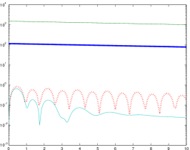
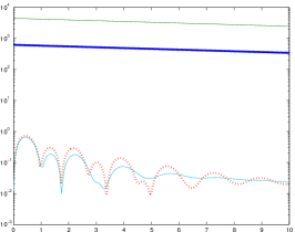
Fig. 1: Upper bound from Corollary 6 (thick, solid), upper bound from Theorem 1, 2-norm of solution $y(t)$ to continuous DDE computed with the Matlab dde23 routine, and 2-norm of solution $y_{n}$ to discretized equation (thick, dotted) for $N=10$ (left), $N=25$ (center), $N=50$ (right).

4 Upper bounds for delay differential equations

Now we turn to transient bounds for DDEs

$$\dot{u}(t)=Au(t)+Bu(t-\tau)\qquad A,B\in\mathbb{C}^{n\times n}$$ (6)

with a single delay $\tau>0$ and with $\alpha(A)$ and $\alpha(T)$ both negative, where $T(z)=zI-A-Be^{-\tau z}$ is the characteristic equation [16]. Although we treat only a single delay here, a direct extension to multiple constant delays is straightforward.

The characteristic equation $T(z)=zI-A-Be^{-\tau z}$ generally has infinitely many eigenvalues, as is often the case with nonlinear matrix-valued functions. Therefore, unlike in the previous section, bounds on transient behavior will depend on integrals whose integration path is unbounded. So, if we expect a bound for a DDE to be useful in practice, then we expect it to require more preparation (such as locating eigenvalues so as to find an admissible integration path) and look more complicated (since the integrand’s behavior at infinity will need to be analyzed) than a bound for an ODE.

Let $\Psi$ be the fundamental solution for the DDE, that is, the solution whose initial conditions are zero on $[-\tau,0)$ and the matrix identity $I$ at $t=0$. Following the treatment in Chapter 1 of [10], we first bound $\Psi$ by invoking the Mellin inversion theorem [20] and then splitting the characteristic equation into its linear and nonlinear parts. We show that the integration can be taken over a curve more convenient than the usual vertical one, and finally compute upper bounds using elementary means.

Lemma 7.

If $X,Y\in\mathbb{C}^{n\times n}$ are two matrices, and if $\|X^{-1}\|\,\|Y\|<1$, then

$$\|(X-Y)^{-1}\|\leq\frac{1}{\|X^{-1}\|^{-1}-\|Y\|}.$$

Proof.

We write $(X-Y)^{-1}=(I-X^{-1}Y)^{-1}X^{-1}$. By hypothesis, the Neumann series $\sum_{j=0}^{\infty}(X^{-1}Y)^{j}$ for $(I-X^{-1}Y)^{-1}$ converges and is bounded by $(1-\|X^{-1}\|\,\|Y\|)^{-1}$. Therefore $\|(X-Y)^{-1}\|\leq\|X^{-1}\|\,(1-\|X^{-1}\|\,\|Y\|)^{-1}$ and the desired result follows. ∎

Lemma 7 can be used to bound $\|T(z)^{-1}\|=\|(zI-A-Be^{-\tau z})^{-1}\|$ in various ways, depending on the choice of norm and the properties of the matrices $A$ and $B$. For simplicity, in the following lemma we use $\|\cdot\|=\|\cdot\|_{2}$ and assume $A$ is Hermitian. Generalizations are straightforward. For instance, the laser example analyzed in this section does not have $A$ Hermitian and we show how to apply our results to that case.

Lemma 8.

Let $T(z)=zI-A-Be^{-\tau z}$ with $A=VDV^{\ast}$ Hermitian. If $y_{0}$ is a given positive number, and $\eta$ is chosen so that

$$1<\eta y_{0}<\min\bigg{\{}\frac{y_{0}}{\|B\|_{2}},e^{-\alpha(T)\tau},e^{-\alpha(A)\tau}\bigg{\}},$$

then

$$\Gamma=\underbrace{\{x(y)+iy:|y|>y_{0}\}}_{\Gamma_{\infty}}\cup\underbrace{\{x_{0}+iy:|y|\leq y_{0},x_{0}=x(y_{0})\}}_{\Gamma_{0}},\qquad x(y)=-\frac{1}{\tau}\log\left(|y|\eta\right)$$

is to the right of both $\Lambda(T)$ and $\sigma(A)$ but lies entirely in the left half-plane.

Proof.

$\Gamma$ is certainly to the right of $\sigma(A)$, since all eigenvalues of $A$ are real and the condition $\eta y_{0}<e^{-\alpha(A)\tau}$ guarantees $x(y_{0})>\alpha(A)$. The eigenvalues of $T$ are also to the left of $\Gamma_{0}$ by the condition $\eta y_{0}<e^{-\alpha(T)\tau}$. As for $\Gamma_{\infty}$, $\|(zI-A)^{-1}\|_{2}^{-1}=\sigma_{\min}(zI-D)\geq|y|$ because the eigenvalues of $A$ are real. Hence, if $z\in\Gamma_{\infty}$, then $\|(zI-A)^{-1}\|_{2}^{-1}\geq|y|>\|B\|_{2}\eta|y|$ by the hypothesis $\eta<1/\|B\|_{2}$. Therefore, Lemma 7 applies with $X=zI-A$ and $Y=Be^{-\tau z}$, so $\|T(z)^{-1}\|\leq\left(|y|-\|B\|_{2}\eta|y|\right)^{-1}<\infty$ on $\Gamma_{\infty}$. Since decreasing $\eta$ to zero moves $\Gamma_{\infty}$ infinitely to the right, and decreasing $\eta$ does not violate the assumption guaranteeing nonsingularity of $T$ on $\Gamma_{\infty}$, it follows that $T$ is nonsingular on and at all points to the right of $\Gamma_{\infty}$. Therefore $\Gamma$ is to the right of $\Lambda(T)$. The condition $1<\eta y_{0}$ assures that $\Gamma_{0}$ is in the left half-plane, and therefore so is $\Gamma$. ∎

By our assumption that all eigenvalues of $T$ are in the left half plane, all solutions of (6) are exponentially stable [16, Proposition 1.6] and hence of exponential order. Therefore we can take the Laplace transform of (6) to obtain

$$(zI-A-Be^{-\tau z})U(z)=u(0)+Be^{-\tau z}\int_{-\tau}^{0}e^{-zt}u(t)\,dt,\quad U=\mathcal{L}u.$$

Since the fundamental solution satisfies $\Psi(t)=0$ on $[-\tau,0)$ and $\Psi(0)=I$, it follows that $(\mathcal{L}\Psi)(z)=T(z)^{-1}$. Then we can use the Mellin inversion theorem [20] to write

$$\Psi(t)=\frac{1}{2\pi i}\int_{\gamma+i\mathbb{R}}T(z)^{-1}e^{zt}\,dz$$ (7)

for any $\gamma>\alpha(T)$. The next lemma shows that we can integrate over the contour $\Gamma$ from Lemma 8 rather than $\gamma+i\mathbb{R}$ in (7).

Lemma 9.

For $\Gamma$ as in Lemma 8 and $\gamma$ such that (7) holds, we have

$$\int_{\Gamma}T(z)^{-1}e^{zt}\,dz=\int_{\gamma+i\mathbb{R}}T(z)^{-1}e^{zt}\,dz.$$

Proof.

Since $T$ has no eigenvalues in the region bounded by $\gamma+i\mathbb{R}$ and $\Gamma$, we only need to show that the integrals

$$\int_{x(y)}^{\gamma}T(w+iy)^{-1}\,e^{(w+iy)t}\,dw$$

go to zero as $y\rightarrow\pm\infty$. But from Lemma 7 we know $\|T(w+iy)^{-1}\|\sim\frac{1}{|y|}$ on $x(y)\leq w\leq\gamma$ as $|y|$ becomes large, and $|e^{(w+iy)t}|\leq e^{\gamma t}$ on the integration path which itself has arc length $\sim\log(|y|)$. Therefore

$$\Bigg{\|}\int_{x(y)}^{\gamma}T(w+iy)^{-1}\,e^{(w+iy)t}\,dw\Bigg{\|}\lesssim\frac{\log|y|}{|y|}\rightarrow 0$$

as $|y|$ becomes large, and the lemma is proved. ∎

We now come to the main result of this section, in which we bound transient growth of the fundamental solution. Note that a bound on $\Psi(t)$ for $t\geq\tau$ is all that is required, since $\Psi(t)=e^{At}$ for $0\leq t<\tau$. Again, we use the 2-norm, but only for simplicity.

Theorem 10.

With the hypotheses of the previous lemmas, the fundamental solution of $\dot{u}(t)=Au(t)+Bu(t-\tau)$ satisfies the bound

$$\|\Psi(t)\|_{2}\leq\|\exp(At)\|_{2}+e^{x_{0}t}I_{0}+e^{x_{0}t}\frac{C}{t/\tau}$$

on $t\geq\tau$, where

$$I_{0}=\frac{1}{2\pi}\int_{-y_{0}}^{y_{0}}\|T(x_{0}+iy)^{-1}-R(x_{0}+iy)\|_{2}dy,\quad R(z)=(zI-A)^{-1}$$

and

$$C=\frac{\|B\|_{2}\eta\sqrt{(\tau y_{0})^{-2}+1}}{\pi\left(1-\|B\|_{2}\eta\right)}.$$

Proof.

Since $\Gamma$ was chosen to the right of all eigenvalues of $A$, the splitting

$$\frac{1}{2\pi i}\int_{\Gamma}T(z)^{-1}e^{zt}\,dz=\frac{1}{2\pi i}\int_{\Gamma}R(z)e^{zt}\,dz+\frac{1}{2\pi i}\int_{\Gamma}\left[T(z)^{-1}-R(z)\right]e^{zt}\,dz$$

and subsequent evaluation of the first summand as $e^{At}$ is justified, as the Mellin inversion theorem applies to $R(z)$ for the same reason it applies to $T(z)^{-1}$. With $I_{0}$ as defined in the theorem statement, it only remains to give a bound on the second integral in the sum.

From the hypothesis that $A$ is Hermitian we have that $\|R(z)\|_{2}\leq|y|^{-1}$, and hence $\|R(z)Be^{-\tau z}\|_{2}\leq\|B\|_{2}\eta$. Therefore the assumption $\eta y_{0}<y_{0}/\|B\|_{2}$ implies $\|R(z)Be^{-\tau z}\|_{2}<1$ on $\Gamma_{\infty}$, so that $T(z)^{-1}-R(z)$ is subject to the Neumann bound

$$\|T(z)^{-1}-R(z)\|_{2}\leq|y|^{-1}\|B\|_{2}\eta\left(1-\|B\|_{2}\eta\right)^{-1}.$$

In addition, if $z\in\Gamma_{\infty}$ then $|z^{\prime}(y)|\leq\sqrt{\left(\tau y_{0}\right)^{-2}+1}$. It then follows that

$$\bigg{\|}\frac{1}{2\pi i}\int_{\Gamma_{\infty}}\left[T(z)^{-1}-R(z)\right]e^{zt}\,dz\bigg{\|}_{2}\leq e^{x_{0}(t-\tau)}\frac{C}{t/\tau}.$$

∎

Remark 4.

In general, if $A$ is not Hermitian we can still bound $\|R(z)\|$ simply by splitting $A$ into its Hermitian and skew-Hermitian parts as $A=H+S$, from which $\|R(z)\|_{2}\leq(|y|-\|S\|_{2})^{-1}$ if we use the 2-norm. However $\|R(z)\|$ is bounded must be taken into account when choosing $\Gamma_{\infty}$.

Also note that we could have integrated over a vertical contour at $\mathfrak{Re}z=x_{0}$, because $\|T(x_{0}+iy)^{-1}-R(x_{0}+iy)\|\lesssim|y|^{-2}$ as $|y|\rightarrow\infty$. But then we obtain

$$\|\Psi(t)\|_{2}\leq\|\exp(At)\|_{2}+e^{x_{0}t}I_{0}+e^{x_{0}t}C,\qquad C=\frac{\|B\|_{2}\eta}{\pi(1-\|B\|_{2}\eta)}$$ (8)

and we have lost the $1/t$ dependence in the third term.

Since $\|T(z)^{-1}\|$ is integrable on $\Gamma_{\infty}$, we also could have obtained an upper bound in terms of the integral of $\|T(z)^{-1}\|$ over $\Gamma_{0}$ and another term with $1/t$ dependence, specifically

$$\|\Psi(t)\|_{2}\leq e^{x_{0}t}\tilde{I_{0}}+e^{x_{0}t}\frac{C}{t/\tau},\qquad\tilde{I_{0}}=\frac{1}{2\pi}\int_{\Gamma_{0}}\|T(z)^{-1}\|_{2}\,|dz|,\ \ C=\frac{\sqrt{(\tau y_{0})^{-2}+1}}{\pi(1-\|B\|_{2}\eta)}.$$ (9)

In this version we fail to take advantage of the closed form of $\int R(z)e^{zt}\,dz$. However, we may be able to shift $x_{0}$ further to the left since we no longer need to have $\Gamma$ to the right of the spectrum of $A$, and this will result in faster decay.

One consequence of a bound on the fundamental solution is a bound on worst-case transient behavior of a certain class of solutions, namely the ones equal to zero on $[-\tau,0)$ and with an initial “shock” condition specified at $t=0$.

Example 2.

Consider the DDE

$$\dot{v}(t)=Av(t)+Bv(t-\tau),\quad\tau=0.2$$ (10)

coming from the discretization of a parabolic partial differential delay equation (adapted from [4, §5.1]), where $n=10^{2}$ and $h=\pi/(n+1)$, and $A,B\in\mathbb{C}^{n,n}$ are defined by

$$A=\frac{1}{h^{2}}\begin{pmatrix}-2&1&\\ 1&\ddots&1\\ &1&-2\end{pmatrix}+\frac{1}{2}I,\qquad B(j,j)=a_{1}(jh),\quad a_{1}(x)=-4.1+x(1-e^{x-\pi}).$$

Rather than compute eigenvalues of $T$ to obtain $\alpha(T)$, we can compute inclusion regions [2, Theorem 3.1] with the splitting $T(z)=D(z)+E(z)$, $D(z)=zI-\Lambda$ diagonal and $E(z)=V^{-1}BVe^{-\tau z}$, where $A=V\Lambda V^{-1}$. The resulting inclusion regions are plotted in Figure 2 (left). The rightmost point of the inclusion regions is then a bound for $\alpha(T)$. The largest eigenvalues of $A$ are also plotted, and the solid contour is chosen as in the theorem, with $y_{0}=21.4214$ and $\eta=0.0491366$, so that it is to the right of both the eigenvalues of $T$ and the eigenvalues of $A$. The dashed contour is the vertical alternate integration path, as referred to in Remark 4. Lastly, if we use (9), we can integrate over a contour whose vertical section is shifted to the left, depicted as the dotted line in Figure 2 (left).

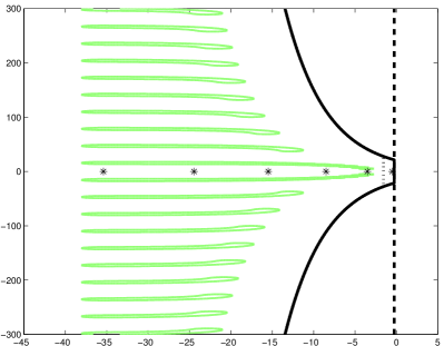
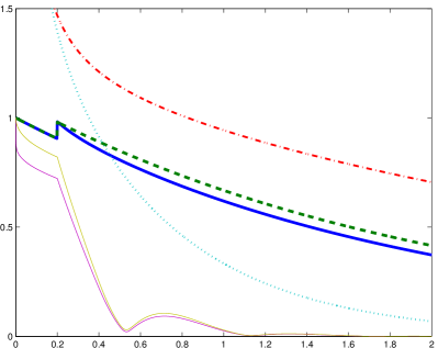
Fig. 2: Left: Inclusion regions for the eigenvalues of $T(z)$ [2], the six largest eigenvalues of $A$, the contour $\Gamma$ used in Theorem 10 (solid), and the vertical contour used for alternate bound (8) (dashed). Contour parameters $y_{0}$ and $\eta$ are set to 21.4214 and 0.0491366, respectively. For the contour with left-shifted vertical part (dotted), $y_{0}=27.7628$ and $\eta=0.0491366$. Right: Upper bounds on the fundamental solution of (10): the upper bound described in the theorem (solid), and the alternates (8) (dashed), (9) (dot-dashed), and (9) with the contour with dotted vertical part (dotted). Lower solid curves are solutions to (10) with zero initial condition on $[-\tau,0)$ and various unit-norm initial conditions specified at $t=0$.

In Figure 2 (right), we have plotted the bound derived using the theorem (solid), as well alternate bounds (8) (dashed), (9) (dot-dashed), and (9) with the contour whose vertical part is shifted leftward (dotted). The last bound gives better results for larger times, as expected, but the bound given in Theorem 10 outperforms it for smaller times and outperforms the other bounds for all times $t>\tau$.

In case $u([-\tau,0))\not\equiv 0$, we can still obtain bounds on $u(t)$ in terms of the fundamental solution $\Psi(t)$.

Corollary 11.

Suppose $u$ satisfies the DDE of the theorem subject to initial conditions $u(0+)=u_{0}$ and $u(t)=\varphi(t)$ on $[-\tau,0)$, with $B\varphi$ integrable. Then

$$\|u(t)\|_{2}\leq\|\Psi(t)\|_{2}\cdot\|u_{0}\|_{2}+\sup_{0\leq\nu<\tau}\|\Psi(t-\nu)\|_{2}\,\int_{0}^{\tau}\|B\varphi(\nu-\tau)\|_{2}\,d\nu.$$

Furthermore, this bound is dominated by the more generous but more explicit piecewise bound $k_{1}(t)\|u_{0}\|_{2}+k_{2}(t)\int_{0}^{\tau}\|B\varphi(\nu-\tau)\|_{2}\,d\nu$, where $k_{1}(t)$ is an upper bound on $\|\Psi(t)\|_{2}$ and

$$k_{2}(t)=\begin{cases}\displaystyle\sup_{0<s<t}\|\exp(As)\|_{2}&(0\leq t<\tau),\\ \displaystyle\sup_{t-\tau<s<\tau}\|\exp(As)\|_{2}+\displaystyle\sup_{\tau<s<t}\|\exp(As)\|_{2}+e^{x_{0}\tau}(I_{0}+C)&(\tau\leq t<2\tau),\\ \displaystyle\sup_{t-\tau<s<t}\|\exp(As)\|_{2}+e^{x_{0}(t-\tau)}\left(I_{0}+\frac{C}{(t-\tau)/\tau}\right)&(t\geq 2\tau).\end{cases}$$

Proof.

From [10, Ch. 1, Thm. 6.1],

$$u(t)=\Psi(t)u_{0}+\int_{0}^{\tau}\Psi(t-\nu)B\varphi(\nu-\tau)\,d\nu$$

and the first assertion is obvious. Using the fact that $\Psi(t)=e^{At}$ on $0\leq t<\tau$ and $\Psi(t-\nu)=0$ for $t-\nu<0$, the integration path can be truncated to $\int_{0}^{t}$. Similarly, if $\tau\leq t<2\tau$, then $\Psi(t-\nu)=e^{A(t-\nu)}$ for $t-\tau<\nu<\tau$, and for this range of $\nu$ we have $t-\nu\geq\tau$. Finally, if $t\geq n\tau$ then $t-\nu\geq(n-1)\tau$ as $\nu\leq\tau$. Taking norms and applying the theorem gives the piecewise bounds. ∎

Example 3.

We return to the model of the semiconductor laser with phase-conjugate feedback. Since $A$ is not Hermitian, Theorem 10 does not apply directly. However, by letting $\beta$ equal the largest imaginary part of any eigenvalue of $A$, changing the definition of $\Gamma_{\infty}$ so that $x(y)=-\log\left(\eta(|y|-\beta)\right)$ instead, and using the fact that $A=VDV^{-1}$ is diagonalizable, it is straightforward to derive the same bound as in Theorem 10 with the alteration

$$C=\frac{\kappa_{2}(V)\eta\|E\|_{2}\sqrt{(\tau(y_{0}-\beta))^{-1}+1}}{\pi(1-\eta\|E\|_{2})},$$

where $E=V^{-1}BV$, $\kappa_{2}(V)$ is the 2-norm condition number of $V$, and $y_{0}$ and $\eta$ were chosen to satisfy

$$1<\eta(y_{0}-\beta)<\min\Bigg{\{}\frac{y_{0}-\beta}{\|E\|_{2}},e^{-\alpha(T)},e^{-\alpha(A)}\Bigg{\}}.$$

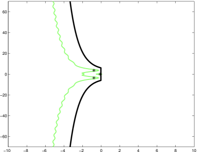
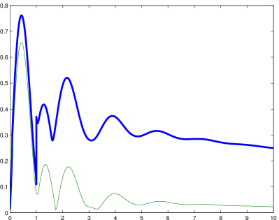
Fig. 3: Left: An inclusion region for the eigenvalues of $T(z)$ [2], the three right-most eigenvalues of $T(z)$, and the contour $\Gamma$ (thick line). Contour parameters $y_{0}$ and $\eta$ are set to 21.4214 and 0.0491366, respectively. Right: Upper bound on solution with initial conditions $\phi(t)\equiv u(0)$ (thick line) and the solution computed with Matlab’s dde23.

Inclusion regions were obtained for $\tilde{T}(z)=zI-\Lambda-Ee^{-z}$ with the splitting $D(z)=zI-\Lambda-E_{0}e^{-z}$ and $E(z)=Fe^{-z}$ ($E_{0}=\mathop{\operator@font diag}\nolimits E$, $F=E-E_{0}$) and an application of Theorem 3.1 in [2]. The one component of the inclusion region intersecting the right half-plane contains exactly one eigenvalue of $D(z)$, and therefore exactly one eigenvalue of $T(z)$, which we have computed using Newton’s method on a bordered system [6, Chapter 3].

5 Lower bounds

The following is an extension of Theorem 2.

Theorem 12.

Suppose we have the representations

$$\Psi(t)=\frac{1}{2\pi i}\int_{\Gamma}T(z)^{-1}e^{zt}\,dz\qquad\text{and}\qquad T(z)^{-1}=\int_{0}^{\infty}\Psi(t)e^{-zt}\,dt$$

where the latter holds for $\mathfrak{Re}(z)>\alpha(T)$, $T$ some matrix-valued function, and $\Gamma$ is a (possibly unbounded) curve in the complex plane. Then for arbitrary $\omega\in\mathbb{R}$,

$$\sup_{t\geq 0}\|\Psi(t)\|e^{-\omega t}\geq\frac{\alpha_{\varepsilon}(T)-\omega}{\varepsilon}$$

for any $\varepsilon>0$ for which $\alpha_{\varepsilon}(T)$ is finite.

Proof.

Suppose $\|\Psi(t)\|\leq Ce^{\omega t}$ for all $t\geq 0$ and fix $\varepsilon>0$. Without loss of generality, suppose that $\omega<\alpha_{\varepsilon}(T)$, and take $z\in\Lambda_{\varepsilon}(T)$ such that $\mathfrak{Re}z>\alpha(T)$ and $\mathfrak{Re}z>\omega$. Then by the representation for $T(z)^{-1}$, the bound on $\Psi(t)$ implies $\|T(z)^{-1}\|\leq\frac{C}{\mathfrak{Re}(z)-\omega}$. Then $\|T(z)^{-1}\|>\varepsilon^{-1}$ by definition of $\Lambda_{\varepsilon}(T)$, which implies $\mathfrak{Re}(z)-\omega<C\varepsilon$. It follows that $\alpha_{\varepsilon}(T)\leq C\varepsilon+\omega$. By the contrapositive, $\alpha_{\varepsilon}(T)>C\varepsilon+\omega$ implies the desired result. ∎

The following proposition is easier to use in practice.

Proposition 13.

For each $x>0$, $\sup_{t\geq 0}\|\Psi(t)\|\geq x\sup_{y\in\mathbb{R}}\|T(x+iy)^{-1}\|$.

Proof.

Fix $x$ and let $y\in\mathbb{R}$ be arbitrary. Set $\|T(x+iy)^{-1}\|=\varepsilon^{-1}$. Then $\alpha_{\varepsilon}(T)\geq x$. From Theorem 12, $\sup_{t\geq 0}\|\Psi(t)\|\geq x\varepsilon^{-1}$. For fixed $x$, the right-hand side is maximized by finding $\varepsilon$ as small as possible, i.e. by finding $y$ such that $\|T(x+iy)^{-1}\|$ is as large as possible. ∎

Remark 5.

Note that for a given $x$ we may only need to check a finite range of $y$ values. This can be shown by proving that for $|y|$ sufficiently large $\|T(x+iy)^{-1}\|\leq\|T(x)^{-1}\|$, for example.

Example 4.

We now give lower bounds on worst-case growth for our two examples. In the case of the discretized PDDE, we use the fact that $A$ is Hermitian to derive $\|T(x+iy)^{-1}\|_{2}\leq\|T(x)^{-1}\|_{2}$ for $|y|>|x|+\|B\|_{2}e^{-\tau x}+\sigma_{\min}(T(x))$ as per the previous remark, and check 100 equally spaced $x$ values in $[5,10]$ for the largest lower bound given by Proposition 13. For the linearization of the laser example, where $A$ is not Hermitian, we use instead that $\|T(x+iy)^{-1}\|_{2}\leq\|T(x)^{-1}\|_{2}$ for $|y|>\|xI-A\|_{2}+\|B\|_{2}e^{-x}+\sigma_{\min}(T(x))$ and check an equally spaced 100 point mesh of $[1,5]$.

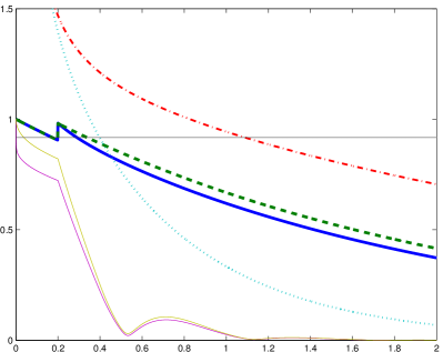
Fig. 4: Left: Discretized PDDE example with lower bound for solutions with $\|u(0)\|_{2}=1$. Notice that one but not both of the plotted solutions for the discretized partial DDE have supremum above the given lower bound. Right: Linearization of laser example with lower bound for solutions with $\|u(0)\|_{2}=0.0015\|(E_{x},E_{y},N)^{T}\|_{2}$. The solution to the linearized system from the laser model departs significantly from the equilibrium before decaying asymptotically. Unless the truncated nonlinear part of the original laser model is guaranteed to stay small under departures which differ from the equilibrium by 0.38242 in norm, the applicability of the linear stability analysis to this equilibrium and these initial conditions is questionable.

6 Conclusion

Some practical, pointwise upper bounds on solutions to higher-order ODEs and single, constant delay DDEs have been demonstrated on a discretized partial DDE and a DDE model of a semiconductor laser with phase-conjugate feedback. A general lower bound was stated and used to concretely bound worst-case transient growth for both examples with a small computational effort. Effective techniques for localizing eigenvalues rather than computing them were used in an auxiliary fashion.

References

[1]A. Bellen and S. Maset, Numerical solution of constant coefficient
linear delay differential equations as abstract cauchy problems, Numerische
Mathematik, 84 (2000), pp. 351–374.
[2]D. Bindel and A. Hood, Localization theorems for nonlinear
eigenvalue problems., SIAM J. Matrix Analysis Applications, 34 (2013),
pp. 1728–1749.
[3]G. Bischi, C. Chiarella, and L. Gardini, Nonlinear Dynamics in
Economics, Finance and the Social Sciences: Essays in Honour of John Barkley
Rosser Jr, Springer, 2009.
[4]C. Effenberger, Robust successive computation of eigenpairs for
nonlinear eigenvalue problems, SIAM Journal on Matrix Analysis and
Applications, 34 (2013), pp. 1231–1256.
[5]T. Gebhardt and S. Grossmann, Chaos transition despite linear
stability, Phys. Rev. E, 50 (1994), pp. 3705–3711.
[6]W. J. F. Govaerts, Numerical Methods for Bifurcations of Dynamical
Equilibria, SIAM, 2000.
[7]G. R. Gray, D. Huang, and G. P. Agrawal, Chaotic dynamics of
semiconductor lasers with phase-conjugate feedback, Phys. Rev. A, 49 (1994),
pp. 2096–2105.
[8]K. Green and B. Krauskopf, Global bifurcations and bistability at
the locking boundaries of a semiconductor laser with phase-conjugate
feedback, Phys. Rev. E, 66 (2002), p. 016220.
[9]K. Green and T. Wagenknecht, Pseudospectra and delay differential
equations, Journal of Computational and Applied Mathematics, 196 (2006),
pp. 567 – 578.
[10]J. Hale and S. Lunel, Introduction to Functional Differential
Equations, no. v. 99 in Applied Mathematical Sciences, Springer, 1993.
[11]D. Hinrichsen and A. Pritchard, Mathematical Systems Theory I:
Modelling, State Space Analysis, Stability and Robustness, Texts in Applied
Mathematics, Springer, 2006.
[12]B. Krauskopf, G. R. Gray, and D. Lenstra, Semiconductor laser with
phase-conjugate feedback: Dynamics and bifurcations, Phys. Rev. E, 58
(1998), pp. 7190–7197.
[13]I. Kubiaczyk and S. Saker, Oscillation and stability in nonlinear
delay differential equations of population dynamics, Mathematical and
Computer Modelling, 35 (2002), pp. 295 – 301.
[14]B. Lehman, Stability of chemical reactions in a cstr with delayed
recycle stream, in American Control Conference, 1994, vol. 3, June 1994,
pp. 3521–3522 vol.3.
[15]B. Lehman, J. Bentsman, S. Lunel, and E. Verriest, Vibrational
control of nonlinear time lag systems with arbitrarily large but bounded
delay: averaging theory, stabilizability, and transient behavior, in
Decision and Control, 1992., Proceedings of the 31st IEEE Conference on,
1992, pp. 1287–1294 vol.2.
[16]W. Michiels and S.-I. Niculescu, Stability and Stabilization of
Time-Delay Systems (Advances in Design & Control) (Advances in Design and
Control), Society for Industrial and Applied Mathematics, Philadelphia, PA,
USA, 2007.
[17]E. Plischke, Transient Effects of Linear Dynamical Systems, PhD
thesis, Universität Bremen, July 2005.
[18]J. R. Singler, Transition to turbulence, small disturbances, and
sensitivity analysis i: A motivating problem, Journal of Mathematical
Analysis and Applications, 337 (2008), pp. 1425 – 1441.
[19]L. Trefethen and M. Embree, Spectra and Pseudospectra: The Behavior
of Nonnormal Matrices and Operators, Princeton University Press, 2005.
[20]H. Weinberger, A First Course in Partial Differential Equations:
with Complex Variables and Transform Methods, Dover Books on Mathematics,
Dover Publications, 2012.