An Adaptive Multiscale Approach for Electronic Structure Methods

Abstract

In this paper, we introduce a new scheme for the efficient numerical treatment of the electronic Schrödinger equation for molecules. It is based on the combination of a many-body expansion, which corresponds to the bond order dissection Anova approach introduced in [35, 42], with a hierarchy of basis sets of increasing order. Here, the energy is represented as a finite sum of contributions associated to subsets of nuclei and basis sets in a telescoping sum like fashion. Under the assumption of data locality of the electronic density (nearsightedness of electronic matter), the terms of this expansion decay rapidly and higher terms may be neglected. We further extend the approach in a dimension-adaptive fashion to generate quasi-optimal approximations, i.e. a specific truncation of the hierarchical series such that the total benefit is maximized for a fixed amount of costs. This way, we are able to achieve substantial speed up factors compared to conventional first principles methods depending on the molecular system under consideration. In particular, the method can deal efficiently with molecular systems which include only a small active part that needs to be described by accurate but expensive models.

1 Introduction

The idea of so-called QM/MM hybrid approaches is to combine highly accurate quantum mechanical (QM) methods and fast molecular mechanics (MM) methods in a cost efficient manner [4]. Such methods make use of the fact that, in many applications, it is sufficient to model a small part of a system in great detail and the rest of the system in less detail only [69, 64]. Numerically, the microscale with its reactive part is usually treated with QM approaches like e.g. Hartree-Fock (HF), configuration interaction (CI), Möller-Plesset (MP2), coupled cluster (CC) or density functional theory (DFT) methods which yield approximate solutions to the underlying quantum-mechanical electronic Schrödinger equation. The mesoscale with its non-reactive part is described by classical MM methods which use Newton’s mechanics with empirically fitted potential functions. Here, one of the main challenges is to define the QM region, the MM region and the interactions between them [4]. The ultimate goal would be a seamless coupling of QM computations where needed and classical MM simulations where sufficient. Such approaches are usually referred to as multiscale methods [59, 13, 14, 9, 54].

In this article, we introduce a new method for a seamless coupling of different models. In our so-called adaptive multilevel BOSSANOVA approach, we follow the idea of general sparse grids to combine, on the one hand, an appropriate many-body expansion and, on the other hand, a hierarchy of models in a cost-efficient manner. The so-called regular sparse grid combination technique [11, 36] is well-known from high-dimensional integration, interpolation and the solution of elliptic PDEs [27, 10]. More generally, the construction of a sparse grid can be formulated as a knapsack problem [10]. Here, the benefit and the cost of each hierarchical surplus in an appropriate hierarchical representation is estimated. Then, a quasi-optimal sparse grid approximation can be achieved [10, 60] by a proper truncation of the hierarchical expansion such that the total benefit is maximized for a given total work load. This procedure can be applied using a priori estimates or a posteriori estimates, like in dimension-adaptive sparse grid approaches [28].

After the presentation of our new approach in a general setting, we discuss the case of the approximation of the Born-Oppenheimer energy in more detail. To this end, we use the systematic bond order dissection Anova (BOSSANOVA) algorithm proposed in [35, 42] and consider a hierarchy of models which results from the use of an appropriate systematically convergent hierarchy of one-electron basis sets, like e.g. cc-pVDZ, cc-pVTZ, cc-pVQZ, cc-pV5Z, cc-pV6Z, …, within a specific QM method like e.g. HF or DFT. We discuss both, a priori truncation schemes and dimension-adaptive algorithms which are based on a local cost model and a posteriori local benefit estimators. We apply our new method to approximate the energy of several molecules, where we are able to achieve substantial speed up factors compared to the conventional electronic structure method. In addition, we apply our new adaptive approaches to three large molecules, which can not be treated with any conventional method at all in a reasonable time.

The remaining article is organized as follows. In Section 2 we briefly summarize the basics of the underlying Schrödinger equation and shortly review additive models. In Section 3 we describe our new multilevel Anova-like decomposition scheme. In Section 4 we give numerical results for a broad range of organic molecules. We conclude with some remarks in Section 5.

2 Additive model approaches

In general, any starting point for an approximation or a coupled model must be the full Schrödinger equation for the electrons and nuclei of the system under consideration. But since the time-dependent Schrödinger equation lives in $3(M+N)+1$ dimensions, where $M$ denotes the number of nuclei and $N$ denotes the number of electrons, a direct numerical treatment is impossible due to the curse of dimension. Thus one has to resort to model approximations. As a first step, in the Born-Oppenheimer molecular dynamics approach, the wave functions of the nuclei and electrons are separated, the subsystem of the nuclei is treated classically with Newton’s mechanics and the remaining $3N$-dimensional electronic Schrödinger equation is further approximated by one of the aforementioned QM methods [54]. The potential needed for Newton’s mechanics is obtained from the electronic solution by the Hellmann-Feynman theorem. Then, the resulting equations of motion for the degrees of freedom of the nuclei, i.e. their positions ${\bf R}$, read as follows:

$$m_{k}\ddot{{\bf R}}_{k}(t)=-\nabla_{{R}_{k}}V^{BO}({\bf Z},{\bf R}(t)),$$ (1)

$$V^{BO}({{\bf Z}},{\bf R}(t)):=\inf_{\|\phi\|=1}\left\{\int\phi^{\ast}({\bf r}){H}_{e}({\bf Z},{\bf R}(t),{\bf r})\phi({\bf r})d{\bf r}\right\}.$$ (2)

Here $V^{BO}$ denotes the Born-Oppenheimer ground state energy and $H_{e}$ denotes the electronic Hamiltonian which reads as

$${H_{e}}({\bf Z},{\bf R},{\bf r}) :={H_{ee}}({\bf Z};{\bf R},{\bf r})+\sum_{i<j}^{M}\frac{Z_{i}Z_{j}}{\mid\mid{R}_{i}-{R}_{j}\mid\mid},$$

$${H_{ee}}({\bf Z},{\bf R},{\bf r}) :=-\frac{1}{2}\sum_{k=1}^{N}\Delta_{{r}_{k}}+\sum_{k<l}^{N}\frac{{1}}{\mid\mid{r}_{k}-{r}_{l}\mid\mid}\!-\!\sum_{k=1}^{N}\sum_{j=1}^{M}\frac{Z_{j}}{\mid\mid{r}_{k}-{R}_{j}\mid\mid},$$

where ${\bf Z}=(Z_{1},\ldots,Z_{M})$) denotes the atomic numbers and ${\bf r}$ are the positions of the electrons. Here, all information on the dynamics of an atomic system is encoded in the associated high-dimensional Born-Oppenheimer potential $V^{BO}$. Note that for neutral or positively charged systems, i.e. $N\leq\sum_{j=1}^{M}Z_{j}$, Zhislin’s theorem states that $V^{BO}({\bf Z},{\bf R})$ is an isolated eigenvalue of finite multiplicity of the operator $H_{ee}({\bf Z},{\bf R},{\bf r})$ for all ${\bf R}$ [26]. Note furthermore that difficulties may in general arise for the Born-Oppenheimer ground-state molecular dynamics from the fact that $\nabla_{\bf R}V^{BO}$ is unbounded (because of Coulomb singularities at nuclei cusps) and from the fact that $\nabla_{\bf R}V^{BO}$ might be discontinuous even away from the positions of Coulomb singularities (because of possible eigenvalue crossings of the electronic Hamiltonian $H_{ee}$) [2]. In the following, we will omit the parameter ${\bf Z}$ if it is clear from the context.

Let us remark that a global electronic QM solution is, at least for larger molecules, still too expensive since conventional methods scale at best with ${O}(M^{3})$ due to the underlying problem of matrix diagonalization. Therefore, specific electronic structure methods [29, 71, 7] are employed which scale linearly and thus overcome this complexity problem. There exist for example divide and conquer DFT [79, 70, 76] and partition DFT (PDFT) [22]. Such approaches are based on a partition of the global system into embedded spatial local parts [44], which can be solved separately and then combined to approximate the global solution. This is also the underlying idea of various decomposition and fragmentation approaches, where the full global electronic structure problem is decomposed into appropriate local subproblems, while the local results are linearly combined to generate a consistent energy expression for the global system [31]. For example, there exist the sum of interactions between fragments computed ab initio procedure (SIBFA) [32], the fragmentation reconstruction method (FRM) [3], the fragment molecular orbital method (FMO) [49, 51, 58], additive model approaches [19, 16] and many-body expansions [18, 1, 72, 12, 66, 67, 53, 30, 17]. Note that the linear scaling QM methods and fragmentation based QM methods all take advantage of a data locality principle which involves the so-called nearsightedness of electronic matter [50, 65].

Although these QM based methods are very powerful, they are still too costly for many applications, where large systems have to be treated with high accuracy. Hence, in order to further reduce the costs without losing much accuracy, one tries to somehow use different levels of models (e.g. HF and CCSD(T)) in a decomposition approach.

For example in incremental methods, a many-body expansion

$$E(R_{1},\ldots,R_{M})=F_{\emptyset}+\sum_{i}F_{\{i\}}(R_{i})+\sum_{i<j}F_{\{i,j\}}(R_{i},R_{j})+\ldots+F_{\{1,\ldots,M\}}(R_{1},\ldots,R_{M}),$$

can be used to couple different models. Here, the leading low-order terms in the many body expansion are treated with a high level method, while all higher-order terms are treated at a low level model [77], like e.g. the multilayer hybrid approach [6], the multilevel fragment-based scheme [83] or the many-body integrated fragmentation technique [74, 5].

There exist several methods, which apply different models to different parts of an atomic system, while combining the results to produce a consistent energy expression. This is the case for example in the conventional QM/MM methods [25] and several variants like e.g. the IMOMM ansatz [57] and the ONIOM approach [75]. The common basic idea of most hybrid QM/MM approaches is to use a sum over two nested regions, like e.g. $\Omega_{2}$ and $\Omega_{1}\subseteq\Omega_{2}$, to represent the total energy as

$${E}_{QM}({\Omega_{2}})\approx{E}_{MM}({\Omega_{2}})+\underbrace{({E}_{QM}({\Omega_{1}})-{E}_{MM}({\Omega_{1}}))}_{\text{model improvement}}.$$ (3)

While all these hybrid methods and fragmentation procedures have promising features, they involve stringent chemical knowledge to choose the regions (or cuts) as best as possible while keeping the underlying ground-state electronic density intact.

Furthermore, in quantum chemistry composite methods [61, 20] an additive model approximation is used to couple different levels of models and different levels of basis sets in a cost-efficient manner. Here, for a low level method $E_{1}$, a high level method $E_{2}$, a small basis set $B_{1}$ and a large basis set $B_{2}$, the energy of the high level method using the large basis, i.e. $E_{2}(B_{2})$, is approximated by the sum

$$E_{2}(B_{2}) \approx E_{1}(B_{1})+\underbrace{(E_{1}(B_{2})-E_{1}(B_{1}))}_{\text{basis set improvement}}+\underbrace{(E_{2}(B_{1})-E_{1}(B_{1}))}_{\text{model improvement}}$$ (4)

$$=E_{1}(B_{2})+(E_{2}(B_{1})-E_{1}(B_{1})).$$

This approximation provides in many cases a substantial reduction of computational costs but results in just a slight degradation of accuracy [55].

Let us remark that the additive approximations (3) and (4) can be used as basic building blocks which lead in a recursive fashion formally to the so-called sparse grid combination technique [11, 36], which is the basis for our new adaptive multilevel BOSSANOVA approach.

3 Adaptive multilevel bond order dissection Anova

First of all, let us note that, in many typical applications, it is sufficient to accurately describe just a restricted specific subdomain of the Born-Oppenheimer surface. Therefore, we assume that the error of the quantity of interest of an approximation $\tilde{V}$ to the Born-Oppenheimer surface $V^{BO}$ can be described by $|\mathcal{E}[V^{BO}-\tilde{V}]|$, where $\mathcal{E}$ is an appropriate linear functional. Examples would be energies, forces or Hessians at specific coordinates or on specific subdomains. In this paper we restrict our numerical experiments to the case of the energy at a specific fixed configuration ${\bf R}$. To this end, one can define $\mathcal{E}[V]$ just by the convolution of $V$ and the delta distribution $\delta$, i.e.

$$\mathcal{E}[V]({\bf R}):=\int V({\bf R}^{\prime})\delta({\bf R}-{\bf R}^{\prime})\,d{\bf R}^{\prime}=V({\bf R})$$

Our new approach is based on the conventional BOSSANOVA method [35, 42] and on a hierarchy of models resulting from sequences of correlation-consistent basis sets that are well-known in quantum-chemistry [21, 24]. These methods are coupled using the idea of the optimized sparse grid technique by balancing benefit-cost ratios of hierarchical surpluses, for details, see [10, 60].

In the following subsections, we will first discuss the so-called complete basis set limit, then recall the conventional BOSSANOVA scheme and finally describe our new multilevel and adaptive multilevel BOSSANOVA schemes. Moreover, we will discuss the estimation of local benefit and local cost associated to a hierarchical surplus whose quotient serves as error indicator in the adaptive scheme.

3.1 Complete basis set limit

Now let us shortly recall the full configuration interaction (FCI) method, which corresponds to the application of the Galerkin scheme for the numerical treatment of the electronic Schrödinger equation (2). To this end, let $B_{1}\subseteq B_{2}\subseteq\ldots$ be a sequence of appropriate finite basis sets of one-electron functions in $\mathcal{H}^{1}(\mathbb{R}^{3}\times\{\pm\tfrac{1}{2}\})$ such that the family $\left\{\operatorname*{span}\{B_{p}\}\right\}_{p\in\mathbb{N}}$ is dense in $\mathcal{L}^{2}(\mathbb{R}^{3}\times\{\pm\tfrac{1}{2}\})$. Then, starting from such a family of one-electron basis functions, Slater determinants (which are generated by the outer anti-symmetric product $\wedge$) are used to construct a family of $N$-electron bases functions and an associated dense family of finite dimensional $N$-electron subspaces $\{\mathcal{V}_{p}\}_{\in\mathbb{N}}$ for the $N$-electron space

$$\mathcal{V}:=\mathcal{H}^{1}(\mathbb{R}^{3}\times\{\pm\tfrac{1}{2}\})^{N}\cap\bigwedge_{i=1}^{N}\mathcal{L}^{2}(\mathbb{R}^{3}\times\{\pm\tfrac{1}{2}\})^{N},$$

for details, see [33, 39, 68]. This leads to an associated family of potential energy functions $\{V^{FCI}_{p}\}_{p\in\mathbb{N}}$. Here, for a fixed ${\bf R}=(R_{1},\ldots,R_{M})$ with pair-wise distinct components, $V^{FCI}_{p}({\bf R})$ is given as

$$V^{FCI}_{p}({\bf R}):=\inf_{\phi\in\mathcal{V}_{p},\|\phi\|=1}\int\phi({\bf r})H_{e}({\bf R};{\bf r})\phi({\bf r})d{\bf r},$$ (5)

which results from the discretization of $\mathcal{V}$ by $\mathcal{V}_{p}$, i.e. from a Galerkin-Ritz approximation of the exact ground-state energy $V^{BO}({\bf R})$ of (2).

In particular, the FCI method fulfills the Rayleigh-Ritz variational principle and thus it holds $V^{BO}({\bf R})\leq V^{FCI}_{p}({\bf R})$. Furthermore, if the exact lowest eigenvalue $V^{BO}({\bf R})$ with associated eigenfunction $\phi^{SE}$ has multiplicity one, then there exist a $p_{0}\in\mathbb{N}$ and functions $\phi^{FCI}_{p}({\bf R})\in\mathcal{V}_{p}$ which solve the discrete Galerkin eigenvalue problem (5) and obey the following error bounds

$$\|\phi^{BO}({\bf R})-\phi^{FCI}_{p}({\bf R})\|_{\mathcal{H}^{1}}\leq C_{1}({\bf R})\inf_{\phi\in\mathcal{V}_{p},\|\phi\|=1}\|\phi^{BO}({\bf R})-\phi\|_{\mathcal{H}^{1}},$$

$$0\leq V^{FCI}_{p}({\bf R})-V^{BO}({\bf R})\leq C_{2}({\bf R})\|\phi^{BO}({\bf R})-\phi^{FCI}_{p}({\bf R})\|_{\mathcal{H}^{1}}^{2}$$

for all $p>p_{0}$, see e.g. [33, 68, 81], where $C_{1}({\bf R})$ and $C_{2}({\bf R})$ denote constants which are independent of $p$. Moreover, since $\phi^{BO}$ is at least in $\mathcal{H}^{1}$ and fulfills certain decay properties, the use of an appropriate sequence of bases of sufficient order leads to an error estimate of type

$$V_{p}^{FCI}({\bf R})-V^{BO}({\bf R})\leq C({\bf R})p^{-2},$$

compare e.g. [81, 82]. In the following, we will assume that, for all $\epsilon>0$, there exists a $p_{\epsilon}\in\mathbb{N}$ with

$$\left|\mathcal{E}[V^{BO}-V^{FCI}_{p_{\epsilon}}]\right|<\epsilon$$

and thus also the convergence of the quantity of interest $\mathcal{E}[V^{BO}]$ is provided. Unfortunately, the applicability of the FCI method is limited by the curse of dimensionality, since the number of involved degrees of freedom grows exponentially with the number of electrons $N$. Using the specific regularity of the electronic eigenfunction and provided that its decay properties are present, this curse of dimension can be circumvented to a certain extent by sophisticated sparse grid techniques. But these methods are still restricted to small systems [81, 34, 52, 80].

Thus, we more generally consider electronic structure methods (ESM) which are also based on a discretization of the one-electron space $\mathcal{H}^{1}(\mathbb{R}^{3}\times\{\pm\tfrac{1}{2}\})$, but represent model approximations to the electronic Schrödinger equation, like in particular HF, CI, CC and DFT. Here, an appropriately chosen family $\{B_{p}\}_{p\in\mathbb{N}}$ of one-electron basis function sets again results in a family of associated potential energy functions $\{V^{ESM}_{p}\}_{p\in\mathbb{N}}$. We furthermore assume that the telescopic series

$$V^{ESM}_{\infty}:=\sum_{p=1}^{\infty}\left(V^{ESM}_{p}-V^{ESM}_{p-1}\right),$$

is point-wise absolute convergent. Then, we can estimate the error of an approximation $V^{ESM}_{p}$ by

$$\left|\mathcal{E}[V^{BO}-V^{ESM}_{p}]\right|\leq\left|\mathcal{E}[V^{BO}-V^{ESM}_{\infty}]\right|+\left|\mathcal{E}[V^{ESM}_{\infty}-V^{ESM}_{p}]\right|,$$ (6)

where $\left|\mathcal{E}[V^{BO}-V^{ESM}_{\infty}]\right|$ is the model error and $\left|\mathcal{E}[V^{ESM}_{\infty}-V^{ESM}_{p}]\right|$ is the discretization error, respectively. In the following, we will just consider the approximation of the so-called complete basis set limit $V^{ESM}_{\infty}$ for a given electronic structure method.

To this end, let us shortly review complete basis set limit extrapolation schemes which are well known in computational chemistry [47]. For a specific system ${\bf R}$ with pair-wise distinct particle coordinates, the procedure is as follows: First, a sequence of energies is computed using an appropriate ESM with a hierarchical sequence of basis sets. Then, these energy values are used to fit a model equation for the error decay and finally this decay model is applied to extrapolate to the complete basis set limit. For example, correlation-consistent basis sets like e.g. cc-pV$n$Z with $n\in\{2,3,4,5,6,\ldots\}$ are appropriate. Note that extensive numerical studies [63, 38, 23, 47] have demonstrated that in many cases the HF energy converges asymptotically as $e^{-n}$ and the correlation energy, i.e. the difference between the HF energy and the total energy, converges as $n^{-3}$, respectively. Here, $n$ is the maximal angular momentum present in the basis set. Since the total energy is a sum of the HF and the correlation energy, the extrapolation to the CBS limit $V^{ESM}_{\infty}({\bf R})=V^{HF}_{\infty}({\bf R})+V^{corr}_{\infty}({\bf R})$ can be done separately for both components [48]. To this end, for the HF limit, exponential formulae are popular [46], like e.g.

$$V^{HF}_{n}({\bf R})=V^{HF}_{\infty}({\bf R})+Ae^{-\alpha n}.$$

For the correlation energy, limit formula are common which involve rational functions [73], like e.g.

$$V^{corr}_{n}({\bf R})=V^{corr}_{\infty}({\bf R})+Bn^{-\beta},$$

often with $\beta=3$. Besides, also other types of formulae are used for extrapolation which involve, e.g., a mixture of an exponential and a squared exponential [62]

$$V^{ESM}_{n}({\bf R})=V^{ESM}_{\infty}({\bf R})+a^{n}e^{-(n-1)}+b^{n}e^{-(n-1)^{2}}.$$

Analogously to such extrapolation schemes, we assume in the following that we have a family of potential functions $\{V_{p}\}_{p\in\mathbb{N}}$ for which it holds

$$\left|\mathcal{E}[V_{p}-V_{p-1}]\right|\lesssim g(p)$$

for the error of a considered quantity of interest, where the series $\sum^{\infty}_{p}g(p)<\infty$ is absolute convergent.

Note here that $g$ represents an upper limit of the decay behavior of the so-called hierarchical surplus [10] which comes into play for a telescopic sum expansion of $V_{\infty}$. Then, we can estimate the approximation error for $p>0$ from above by

$$\left|\mathcal{E}[V_{p}-V_{\infty}]\right|\lesssim\sum^{\infty}_{p^{\prime}>p}g(p^{\prime}).$$

3.2 BOSSANOVA

Next, let us shortly recall the bond order dissection Anova (BOSSANOVA) approach as introduced in [35, 42]. To this end, we introduce the notation

$$V_{p}(X_{1},\ldots,X_{M}):=V_{p}({\bf Z},{\bf R}),\quad{X}_{i}:=(Z_{i},R_{i}),$$

which denotes the energy computed with a specific ESM at level $p$ of the charge neutral system that consists of $N=\sum^{M}_{i}Z_{i}$ electrons and $M$ nuclei, each with coordinate vector $R_{i}\in\mathbb{R}^{3}$ and atomic number $Z_{i}\in\mathbb{N}$. We now decompose the energy $V_{p}$ into a multivariate telescopic sum, i.e. as a finite series expansion in the nucleic parameters, in a similar way as in the Anova decomposition. The analysis of variance (Anova) approach is well-known from statistics and is closely related to the high-dimensional model representation (HDMR) [40], the multimode approach [15] and many-body expansions [66]. This decomposition involves a splitting of the high-dimensional function into contributions which depend on the positions of single nuclei and associated charges, of pairs of nuclei and associated charges, of triples of nuclei and charges, and so on. Here, we consider the subset of the nuclei parameters $\{{X}_{i}\}_{i\in u}$ described by a set of labels $u\subseteq\{1,\ldots,M\}$ with cardinality $|u|=k$ and call it the molecular fragment associated to $u$ with size $k$. Then, we consider the many-body expansion of $V_{p}$ by

$$V_{p}({X}_{1},\ldots,{X}_{M}) =w_{p,\emptyset}+\sum^{M}_{i_{1}}w_{p,\{i_{1}\}}({X}_{\{i_{1}\}})+\sum^{M}_{i_{1}<i_{2}}w_{p,\{i_{1},i_{2}\}}({X}_{\{i_{1},i_{2}\}})+\ldots$$

$$\quad\quad\ldots+w_{p,\{i_{1},\ldots,i_{M}\}}({X}_{\{i_{1},\ldots,i_{M}\}})$$

$$=\sum_{u\subseteq\{1,\ldots,M\}}w_{p,u}({X}_{u})$$ (7)

where $X_{u}$ denotes the set of variables $\{X_{i}\}_{i\in u}$ and $u\subseteq\{1,\ldots,M\}$. Each term $w_{p,u}$ is defined by an inclusion-exclusion-type combination of potential functions that belong to all associated fragments by

$$w_{p,u}({X}_{u}):=\sum_{v\subseteq u}(-1)^{|u|-|v|}\widehat{V}_{p,v}({X}_{v}).$$ (8)

Alternatively it can recursively defined as

$$w_{p,u}({X}_{u}):=\widehat{V}_{p,u}({X}_{u})-\sum_{k=0}^{|u|-1}\sum_{v\subseteq u,|v|=k}w_{p,v}({X}_{v}).$$ (9)

The constant function $w_{p,\emptyset}$ is set equal to zero since it corresponds to the energy of an empty molecular system. Here, $\widehat{V}_{p,u}({X}_{u})$ should be an approximation to the energy associated with fragment ${X}_{u}$, where the fixed level $p$ relates to the basis set order used by the ESM, and therefore to the accuracy it can achieve. Note at this point that we set

$$\widehat{V}_{p,{\{1,\ldots,M\}}}({\bf X}):=V_{p}({\bf X}),$$ (10)

whereas in general all $\widehat{V}_{p,u}$ with $|u|<M$ could be chosen arbitrarily since (7) and (8) amount to just the identity. Thus, independent of the specific definition of $\widehat{V}_{p,u}$ for $|u|<M$, decomposition (7) is exact and contains $2^{M}$ different terms due to the power set construction, i.e. $u\subseteq\{1,\ldots,M\}$.

In case of a general splitting it might be that all terms $w_{p,u}$ are equally important. But let us now assume that there is a decay of the terms $|\mathcal{E}[w_{p,u}]|$ with increasing order $|u|$. Then, a suitable truncation of the sum (7) opens the possibility to avoid the curse of dimensionality. For example, if for a small $k<M$ all higher order terms $w_{p,u}$ with $|u|>k$ vanish, only the lower dimensionality of the $k$th order terms, i.e. the effective dimension, exponentially enters the work count complexity.

It was observed in [35] that, for a proper choice of the $\widehat{V}_{p,u}$ as good approximation to the ground-state energy associated to the submolecule $X_{u}$, the hierarchical surpluses $w_{p,u}$ indeed decay for most organic molecules fast with their order $k=|u|$. Thus, a proper truncation of the series expansion (7), e.g.

$$\sum_{u\subseteq\{1,\ldots,M\},|u|\leq k}w_{p,u}({X}_{u}),$$

results in a substantial reduction in computational complexity. We then only have to deal with a sequence of lower-dimensional subproblems which are associated to the remaining lower-dimensional energy terms of the decomposition. This leads us to the following assumption which is central to our further approach: The associated energy functions $\widehat{V}_{p,u}$ for $|u|<M$ can be chosen properly such that there is a certain decay in the contribution of each order $k=|u|$ of the Anova expansion which results in a monotone convergence of the approximation error with rising order. Consequently, from a certain order onward, we may neglect the higher higher-order terms in the Anova decomposition. Let us remark that the energy contribution functions $w_{p,u}$ in (7) may be recognized as an expansion of many-body interaction contributions, as in [56], and thus our assumption on the decay is also strongly supported by the success of conventional two- and many-body potential functions used in classical molecular dynamics [72, 18, 8, 37].

Let us now discuss our specific choice of $\widehat{V}_{p,u}(X_{u})=V_{p}(X_{u})$ according to the BOSSANOVA approach as presented in [35, 42], which is aimed at the approximation of the potential energy surface of a molecule. A simple choice would be to set $\widehat{V}_{p,u}(X_{u})=V_{p}(X_{u})$ for all $u\subseteq\{1,\ldots,M\}$. However, the involved cutting of molecules into fragments may break bonds. Furthermore, a cut-out fragment may have a total spin unequal zero while the molecular system itself has a total spin of zero. This situation would complicate the proposed linear-scaling ansatz and usually would result in a slow decay with bond order $k$ of the terms in the many-body expansion (7). A way to remedy this situation is a saturation of the dangling bonds of the fragments by adding hydrogen at the places where bonds were cut, causing the total spin of each augmented fragment system to be zero. This way, only closed-shell calculations are performed, which are algorithmically both simpler and more stable.

To be more precise, let $G=(P,E)$ be the graph which is associated to the organic molecule under consideration and which represents the bond structure of the molecule. For reasons of simplicity we assume that this graph is connected. Then, a saturation procedure for a molecular fragment associated to subset $u$ can be described by $h^{G}(u)$ additional hydrogen vertices, bonds and their graph-dependent positions $R^{G}_{i}(u)$, $1\leq i\leq h^{G}(u)$. Note here that each set $u=\{i_{1},\ldots,i_{|u|}\}$ of indices of nuclei is directly associated to an induced subgraph $G_{u}=({P}_{u},{E}_{u})$ of the total graph $G$ with ${P}_{u}=\{v_{i}\}_{i\in u}$ and $E_{u}=\{\{v_{1},v_{2}\}\subseteq K\,:\,v_{1}\in u,v_{2}\in u\}$. Now, for a subset $u$ with a connected induced subgraph $G_{u}$, we define a modified energy function by

$$\widehat{V}^{G}_{p,u}({X}_{u}):=V_{p}\left({X}_{i_{1}},\ldots,{X}_{i_{|u|}},R^{G}_{1}(u),\ldots,R^{G}_{h^{G}(u)}(u)\right),$$ (11)

while, according to (10), we keep the energy for the total system unmodified, i.e.

$$\widehat{V}^{G}_{p,\{1,\ldots,M\}}({\bf X}):={V}_{p}({\bf X}).$$

This saturation correction is described in detail in [35, 42]. In the case of a subset $u$ where the induced subgraph $G_{u}$ decomposes into at least two connected components,, we define the modified energy function $\widehat{V}^{G}_{p,u}$ as the sum over the modified energy of all connected components of $G_{u}$. It follows in particular that the corresponding hierarchical surplus $w_{p,u}$ indeed vanishes. This is discussed in more detail in Appendix A. This elimination step is motivated by the locality of the electronic wave functions: Atoms that share a bond with a nearby atom will be strongly influenced by changes in the chemical vicinity of nearest or next-nearest bonding partners whereas atoms that share no bond to a nearby atom will not.

Altogether, to a given appropriate bond or interaction graph $G$, we define the conventional BOSSANOVA approximation energy up to order $k$ by

$$V^{\text{BN}}_{p,k}({\bf X}):=\sum_{k^{\prime}\leq k}D_{p,k}^{G}({\bf X}).$$ (12)

Here, $D_{p,k}^{G}$ denotes the hierarchical surplus according to bond order $k$, which is the sum of all $w_{p,u}^{G}$ of bond order $k=|u|$ and level $p$, i.e.

$$D_{p,k}^{G}({\bf X}):=\sum_{u\subseteq\{1,\ldots,M\},|u|=k}w_{p,u}^{G}({X}_{u}),$$ (13)

where $w_{p,u}^{G}({X}_{u})$ is given by (8) using the modified energy functions $\widehat{V}^{G}_{p,u}$ from (11). Note that in [35, 42] the conventional BOSSANOVA approach has been successfully applied to a large range of organic molecules where in most cases a systematic decay of the size of the decomposition terms $D_{p,k}^{G}$ with an increase of the order $k=|u|$ has been observed. In the following we will omit the parameter $G$ to simplify notation.

The BOSSANOVA approach is general in the sense that the local energies can be approximated with any electronic structure method at hand, e.g. HF, CI, CC or MP. This is often referred to as a non-intrusive approach, which means that existing methods and their implementation can be re-used straightforwardly without any modifications. Let us finally remark that the BOSSANOVA method can not be directly applied to metallic systems, since the necessary assumptions do not hold there, a further discussion is given in [42].

3.3 Multilevel BOSSANOVA

Now, we describe our new approach to couple the two different approximation schemes according to (6) and (12), respectively. Here, the idea is to introduce an approximation that is associated to the two corresponding discretization parameters $p$ and $u$, where for each single parameter, a systematic improvement of the approximation is expected. Then, we follow the basic idea of sparse grids [10] and decompose the associated energy approximation in a telescopic sum like fashion and finally truncate the expansion in such a way that its local error and cost contributions are balanced, for details see [10, 60].

3.3.1 Hierarchical series expansion

Up to this point we used the same basis set of fixed degree $q$ for all BOSSANOVA terms $w_{q,u}$. Now we employ electronic structure methods with basis sets of varying order $p\in\mathbb{N}$ to approximate the subsystem’s ground state energies $\widehat{V}_{p,u}$. To this end, we further decompose the conventional BOSSANOVA terms (8) with fixed basis set order $q$ as

$$w_{q,u}({X}_{u})=\sum_{p=0}^{q}\omega_{p,u}({X}_{u}),$$

where the hierarchized ANOVA terms $\omega_{p,u}$ are given by

$$\omega_{p,u}({X}_{u}):=w_{p,u}({X}_{u})-w_{p-1,u}({X}_{u}),$$ (14)

with $w_{-1,u}=0$. We further assume that the series

$$V_{\infty}({X}_{1},\ldots,{X}_{M}):=\sum_{p\in\mathbb{N}}\sum_{u\subseteq\{1,\ldots,M\}}\omega_{p,u}({X}_{u})$$ (15)

is point-wise absolute convergent. Then, according to definition (10), it holds $V_{\infty}=V^{EMS}_{\infty}$. An example of such a decomposition which corresponds to a linear molecule of length three is given in Appendix B.

Analogously, we can define hierarchical surpluses

$$\Delta_{p,k}({\bf X}):=D_{p,k}({\bf X})-D_{p-1,k}({\bf X}),$$ (16)

with $D_{p,k}$ from equation (13) for $p\in\mathbb{N}$ and $D_{-1,k}=0$ and obtain an alternative hierarchical series representation of the complete basis set limit in the form

$$V_{\infty}({X}_{1},\ldots,{X}_{M})=\sum_{p\in\mathbb{N}}\sum_{0\leq k\leq M}\Delta_{p,k}({\bf X}).$$ (17)

Here, (15) is a multilevel expansion with contributions associated to the indices $(p,u)\in\mathbb{N}\times\mathcal{P}(\{1,\dots,M\})$, while expansion (17) is a multilevel expansion with contributions associated to the indices $(p,k)\in\mathbb{N}\times\{0,\dots,M\}$.

3.3.2 General multilevel approximation

Now, we can truncate the infinite sum (17) that represents the complete basis set limit using a properly chosen downward-closed index set ${I}\subseteq\mathbb{N}\times\{1\ldots,M\}$ and obtain

$$V_{I}({\bf X}):=\sum_{(p,k)\in{I}}\Delta_{p,k}({\bf X})$$ (18)

as an approximation to $V_{\infty}({\bf X})$. Here, in the most simple case, the index set $I$ can be chosen as

$$I^{TD}_{L,a}:=\left\{(p,k)\,:\,ap+k\leq L\right\},$$ (19)

i.e. as an $\ell_{1}$-ellipse with scaling parameter $L$ which is related to the desired accuracy and where $a$ prescribes a certain weighting between $p$ and $k$.

Alternatively, a more general approximation than (18) can be obtained by truncation of the infinite hierarchical series (15) using a properly chosen downward-closed index set $\mathcal{I}\subseteq\mathbb{N}\times\mathcal{P}(\{1,\ldots,M\})$, i.e.

$$V_{\mathcal{I}}({\bf X}):=\sum_{(p,u)\in{\mathcal{I}}}\omega_{p,u}({\bf X}).$$ (20)

Note that the concept of downward-closedness is applicable here, since the power set is a partially ordered set. Note furthermore that every approximation (18) can be expressed in form of approximation (20), but this does not hold vice versa.

Now, let us shortly discuss the cost involved in the approximations (18) and (20), respectively. To this end, we assume that the local energies $\widehat{V}_{p,u}({X}_{u})$ are computed with a cost of

$$c(p,u).$$ (21)

Then, it is clear that the cost of computing a term $\omega_{p,u}$ is $\mathcal{O}(c(p,u))$, because all values $\widehat{V}_{p,u}({X}_{u})$ for $v\subsetneq u$ have been computed before, due to the downward-closedness of $\mathcal{I}$. Therefore, the total cost of employing the multilevel BOSSANOVA method (20) with a predefined index-set $\mathcal{I}\subseteq\mathbb{N}\times\mathcal{P}(\{1,\ldots,M\})$ is given by

$$Cost(\mathcal{I})=\sum_{(p,u)\in\mathcal{I}}c(p,u).$$

Analogously, in case of (18) with $I\subseteq\mathbb{N}\times\{0,\ldots,M\}$ the total cost read as

$$Cost(I)=\sum_{(p,k)\in I}C(p,k),$$

where

$$C(p,k):=\sum_{|u|=k}c(p,u).$$ (22)

The advantage of the multilevel BOSSANOVA method stems from neglecting the energy contributions and thus the costs of the less relevant subproblems.

3.3.3 Quasi-optimal approximations

Let us now discuss a proper choice of a finite index sets with respect to an appropriate benefit-cost setting similar to the sparse grid construction [10]. Here, for reasons of simplicity, we will discuss in detail the case of a finite index set ${I}$ in expansion (18) only. The case of a set $\mathcal{I}$ works analogously. To this end, let us assume that it holds $V_{\infty}=V_{\infty}^{EMS}$ and that

$$|\mathcal{E}[\Delta_{p,k}]|\lesssim B(p,k),$$ (23)

where $B:\mathbb{N}\times\{0,\ldots,M\}\to\mathbb{R}_{+}$ denotes an upper bound of $|\mathcal{E}[\Delta_{p,k}]|$, which we call the local benefit. Then, we obtain the upper estimate

$$|\mathcal{E}[V_{\infty}^{EMS}-V_{I}]|=|\mathcal{E}[\sum_{(p,k)\in\mathbb{N}\times\{0,\ldots,M\}\setminus{I}}\Delta_{p,k}]|\lesssim\sum_{(p,k)\in\mathbb{N}\times\{0,\ldots,M\}\setminus{I}}B(p,k).$$ (24)

Let us further assume that the cost contribution associated with a hierarchical surplus $\Delta_{p,k}$ can be estimated from above by an appropriate local cost function $C:\mathbb{N}\times\{1,\ldots,M\}\to\mathbb{R}_{+}$, compare (22).

Now, we assume that we are allowed to spend just a limited total specific cost. Then, the goal is to determine an index set (with at most this associated total cost) such that the overall benefit is maximized. The corresponding associated binary knapsack problem consists in the determination of an index set ${I}_{\text{opt}}\subset\mathbb{N}\times\{0,\ldots,M\}$ that maximizes the total benefit under the constraint of a maximally allowed total cost $C_{max}$, i.e.

$$\max_{{I}}\sum_{(p,k)\in{I}}B(p,k)\quad\text{with}\quad\sum_{(p,k)\in{I}}C(p,k)\leq C_{\text{max}}.$$ (25)

Its solution can be reduced to the discussion of the local benefit-cost ratios $\frac{B(p,k)}{C(p,k)}$. Those indices $(p,k)$ with the largest benefit-cost ratios are taken into account first. This is similar in spirit to the best $n$-term approximation. In the framework of Sobolev spaces of dominating mixed smoothness such a construction leads e.g. to quasi-optimal sparse grids. For a more detailed discussion see e.g. [10, 28, 60]. Note that the described construction is called quasi-optimal [60], since, amongst other issues, the estimate of the total error (24) involves the triangle inequality only but no norm-equivalency.

Analogously to (25), the problem of the determination of an index set $\mathcal{I}_{\text{opt}}\subset\mathbb{N}\times\mathcal{P}(\{1,\ldots,M\})$ that maximizes the total benefit $\sum_{(p,u)\in{\mathcal{I}_{\text{opt}}}}b(p,u)$ under the constraint of maximal allowed total cost $\sum_{(p,u)\in{\mathcal{I}_{\text{opt}}}}c(p,u)\leq C_{\text{max}}$ reduces to the discussion of local benefit-cost ratios $\frac{b(p,u)}{c(p,u)}$.

3.3.4 Local cost model

In electronic structure calculations with standard correlation consistent cc-pV$n$Z basis sets, the number of one-electron basis functions per atom scales as [43, 38, 73]

$$N_{\text{cc-pV$n$Z}}=\tfrac{1}{3}(n+1)(n+\tfrac{3}{2})(n+2).$$ (26)

Roughly speaking, the number of basis functions in the cc-pV$n$Z basis sets grows with third order, i.e. $n^{3}$. In this article, we consider a hierarchy of models which results from the basis sets cc-pV$n$Z with $n\in\{3,4,5,6,\ldots\}$ of Dunning et al. [21, 78]. Here, cc-pVTZ corresponds to the energy level $p=0$, cc-pVQZ corresponds to the energy level $p=1$, cc-pV5Z corresponds to the energy level $p=2$ and cc-pV6Z corresponds to the energy level $p=3$. Higher values of $p$ correspond to better quality.

Furthermore, we assume that the cost of the applied electronic structure method, e.g. HF and DFT, scales with third order in the number of one-electron basis functions. Hence, we estimate the cost of a single calculation for an $M$-atomic molecule by

$$Cost(M,n)\lesssim M^{3}n^{9},$$

in case of HF and DFT, respectively. Note that there are several energy evaluations involved in the computation of a hierarchical surplus $\omega_{p,u}$. However, as already noted in the previous sections, we assume that the computations for all backward neighbors in definition (14) have already been performed and their results have been stored by a simple book-keeping procedure once and for all. Thus, we assume that the local cost according to (21) can be estimated by

$$c(p,u)\leq\beta|u|^{3}(p+3)^{9},$$ (27)

where $\beta$ denote method dependent constant. Note that we neglect here the additional hydrogen atoms resulting from the saturation scheme.

3.4 Adaptive multilevel BOSSANOVA

To construct a quasi-optimal approximation as in Section 3.3.3, a priori local cost and benefit estimators are needed. Let us now discuss the case when there is no suitable a priori estimate for the local benefit available. Then, a possible methodology are so-called dimension-adaptive approaches, which are adaptive greedy-type algorithms using a posteriori estimates [28]. Under the assumption that the benefit-cost ratios obey some kind of appropriate decay, these type of algorithms try to find quasi-optimal index sets in an iterative procedure. To this end, as always for an adaptive heuristics, two main ingredients are needed – an error indicator and a refinement rule. Here we propose a hybrid a priori/a posteriori approach, since we determine the local benefit a posteriori and the local cost a priori.

3.4.1 Adaptive index sets in $\mathbb{N}\times\{0,\ldots,M\}$

First, we introduce Algorithm 1 which builds up a set of indices $(p,k)$ such that the infinite sum (17) is approximated by a quasi optimal approximation (18) up to the desired accuracy at minimal cost. To this end, we refine in each step of our approach the current index set $I$ by adding those indices $(p,k)\in\mathbb{N}\times\{0,\ldots,M\}\setminus I$ with a benefit-cost ratio greater or equal than an a priori chosen factor $[1-\alpha]$ times the highest benefit-cost ratio $\max_{(p,k)\in A}\eta(p,k)$. Here, it is not necessary to consider all of the possible candidates $(p,k)\in\mathbb{N}\times\{0,\ldots,M\}\setminus I$ (which would be too many), but in each iteration step we only take those indices into account which are in the direct neighborhood of the actual set $I_{\alpha}$ and which result in downward-closed sets. Algorithm 1 uses the local cost estimate (22) and computes the local benefit a posteriori according to (23) by

$$|\mathcal{E}[\Delta_{p,k}]|.$$

Thus, for an index $(p,k)\in\mathbb{N}\times\{0,\ldots,M\}$, the associated benefit-cost ratio is given by

$$\eta(p,k):=\frac{|\mathcal{E}[\Delta_{p,k}]|}{C(p,k)}.$$ (28)

Altogether, to a given factor $\alpha\in[0,1]$ and a maximal cost $C_{max}$, Algorithm 1 tries to generate a quasi-optimal index set $I_{\alpha}$ and an associated approximation

$$V_{{I}_{\alpha}}({\bf X}):=\sum_{(p,k)\in{I}_{{\alpha}}}\Delta_{p,k}({\bf X}).$$ (29)

Algorithm 1 Adaptive algorithm to construct a quasi-optimal index sets ${I}_{\alpha}\subseteq\mathbb{N}\times\{0,\ldots,M\}$ for a molecule with interaction graph $G$ to a given maximal allowed cost $C_{max}$, where $\alpha\in[0\,1]$ is an input parameter.

  Initialize: ${I}_{\alpha}:=\emptyset$, $cost:=0$, ${A}:=\{(0,1)\}$

  while $cost<C_{max}$ do

     

1. Compute the values $\eta(p,k):=|\mathcal{E}[\Delta_{p,k}]|/C(p,k)$ for all $(p,k)\in A$ for which $\eta(p,k)$ has not been computed yet and set $cost:=cost+C(p,k)$ respectively.

2. Select new indices $\{(p,k)\in A\,:\,\eta(p,k)\geq(1-\alpha)\max_{(q,l)\in A}\eta(q,l)\}$ and move them from $A$ to $I$.

3. Generate new admissible active index set $A$ for $I_{\alpha}$, i.e. $A:=\{(p,k)\in\mathbb{N}\times\{0,\ldots,M\}\setminus{I}_{\alpha}\,:\,(p,k)\cup{I}_{\alpha}\text{ is downward-closed}\}$

  end while

3.4.2 Adaptive index sets in $\mathbb{N}\times\mathcal{P}(\{1,\ldots,M\})$

An alternative algorithm, which provides the application of different basis sets at different local parts of a molecule is as follows: Instead to rely on set of indices $I\subseteq\mathbb{N}\times\{0,\ldots,M\}$ as before, we now construct an index-set $\mathcal{I}\subseteq\mathbb{N}\times\mathcal{P}(\{1,\ldots,M\})$, considering the whole power set $\mathcal{P}(\{1,\ldots,M\})$ of $\{1,\ldots,M\}$. This allows a much better adaption to the specific molecule in consideration. This straightforward generalization of Algorithm 1 is presented in Algorithm 2.

In contrast to Algorithm 1, Algorithm 2 is based on the expansion (15) and uses benefit-cost ratios associated with indices $(p,u)\in\mathbb{N}\times\mathcal{P}(\{1,\ldots,M\})$ defined by

$$\theta(p,u):=\frac{b(p,u)}{c(p,u)},$$ (30)

where the local benefit is defined by

$$b(p,u):=|\mathcal{E}[\omega_{p,u}]|$$

and the local cost is given according to (21). Analogously to Algorithm 1, Algorithm 2 tries to generate a quasi-optimal index set $\mathcal{I}_{\alpha}$ where the corresponding approximation is given by

$$V_{\mathcal{I}_{\alpha}}({\bf X}):=\sum_{(p,u)\in\mathcal{I}_{{\varepsilon_{i}}}}\omega_{p,u}({X}_{u}).$$ (31)

Algorithm 2 Adaptive algorithm to construct a quasi-optimal index sets $\mathcal{I}_{\alpha}\subseteq\mathbb{N}\times\mathcal{P}({\{1,\ldots,M\}})$ for a molecule with interaction graph $G$ to a given maximal allowed cost $C_{max}$, where $\alpha\in[0\,1]$ is an input parameter.

  Initialize: $\mathcal{I}_{\alpha}:=\emptyset$, $cost:=0$, $\mathcal{A}:=\{(0,1)\}$

  while $cost<C_{max}$ do

     

1. Compute the values $\theta(p,u):=|\mathcal{E}[\omega_{p,u}]|/c(p,u)$ for all $(p,u)\in\mathcal{A}$ for which $\theta(p,u)$ has not been computed yet and set $cost:=cost+c(p,u)$ respectively.

2. Select new indices $\{(p,u)\in\mathcal{A}\,:\,\theta(p,u)\geq(1-\alpha)\max_{(q,v)\in\mathcal{A}}\theta(q,v)\}$ and move them from $\mathcal{A}$ to $\mathcal{I}$.

3. Generate new admissible active index set $\mathcal{A}$ for $\mathcal{I}_{\alpha}$, i.e. $\mathcal{A}:=\{(p,u)\in\mathbb{N}\times\mathcal{P}({\{1,\ldots,M\}})\setminus\mathcal{I}_{\alpha}\,:\,(p,u)\cup\mathcal{I}_{\alpha}\text{ is downward-closed}\}$

  end while

Let us finally remark that in contrast to the relation (22) for the local costs $C(p,k)$ and $c(p,k)$, the local benefit $|\mathcal{E}[\Delta_{p,k}]|$ is not equal to the associated sum of local-benefits $\sum_{u\subseteq\{1,\ldots,M\},|u|=k}b(p,u)$.

3.4.3 Parallel cost model

Note here that using a simple book-keeping procedure, all involved energy evaluations $\widehat{V}_{p,u}({X}_{u})$ only have to be computed once and for all and can in particular be performed in parallel. In such a parallel cost model, the total cost of employing the multilevel BOSSANOVA method with a predefined index-set ${I}\subset\mathbb{N}\times\{0,\ldots,M\}$ can be estimated from above by

$$C^{PA}({I}):=\max_{(p,k)\in{I}}\max_{u\subseteq\{1,\ldots,M\},|u|=k}c(p,u).$$

Analogously, the total costs in case of a predefined index-set $\mathcal{I}\subset\mathbb{N}\times\mathcal{P}(\{1,\ldots,M\})$ can be estimated from above by

$$C^{PA}(\mathcal{I}):=\max_{(p,u)\in\mathcal{I}}c(p,u).$$

In case of the adaptive Algorithm 2 all benefits and respective benefit-cost ratios can be computed in parallel in step 1 of the while loop. Therefore, the total cost of Algorithm 2 in the parallel cost model can be computed by setting $cost:=cost+\max_{(p,u)}c(p,u)$ in step 1 of the while loop. In an analogous way Algorithm 1 can also be modified according to the parallel cost model.

4 Numerical experiments

Now we present the results of our numerical experiments. This section is divided into two parts. In the first part, we perform a numerical study on the decay properties of the hierarchical surpluses of several molecules. In the second part, we will present and discuss the numerical results corresponding to the different approximation approaches which were presented in Section 3.

In all involved electronic structure calculations we apply the Massively Parallel Quantum Chemistry (MPQC) Program [45]. In addition, we use the software package MoleCuilder - a molecular builder [41] for the fragmentation and saturation process involved in the various multilevel BOSSANOVA approaches. Moreover, in the numerical experiments applying the DFT method we use the common B3LYP exchange-correlation functional.

4.1 Numerical study of benefit-cost ratios

In a first step we analyze the benefit-cost ratios $\eta(p,k)$, involved in Algorithm 1, which are defined according to (28). We first study two small molecules. Our results for heptane ($C_{7}H_{16}$ - a small linear molecule) and acrylamide ($C_{3}H_{5}NO$ - a small molecule with branches) applying the HF method within the decomposition (17) are given in Figure 1.

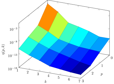
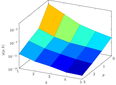
Figure 1: Benefit-cost ratios $\eta(p,k)$ using the HF method corresponding to basis sets cc-pVTZ to cc-pV6Z, i.e. $p=0,\dots,3$. Left: heptane ($C_{7}H_{16}$). Right: acrylamide ($C_{3}H_{5}NO$).

We clearly see that the benefit-cost ratios $\eta(p,k)$ decay with $p+k$ and are in particular approximately constant along the lines $l=p+k$ for a given fixed $l$. This corresponds to the decay behavior in the regular sparse grids case.

Moreover, for acrylamide, acetanilide ($C_{8}H_{9}NO$ - a small molecule with a ring structure) and several alkanes ($C_{5}H_{12}$, $C_{6}H_{14}$, $C_{7}H_{14}$, $C_{20}H_{42}$), we depict the benefit-ratio $\eta(p,k)$ in dependence of the sum $p+k$ in Figure 2.

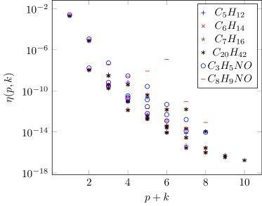
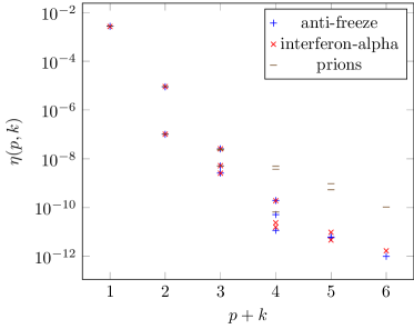
Figure 2: Benefit-cost ratios $\eta(p,k)$ versus the sum $p+k$ for several alkane, acrylamide ($C_{3}H_{5}NO$), acetanilide ($C_{8}H_{9}NO$) applying the HF method (left) and three proteins applying the DFT approach (right).

In addition, we show there the benefit-cost ratio $\eta(p,k)$ for three large molecules, i.e. an anti-freeze protein (992 atoms), an interferon-$\alpha$ protein (2698 atoms) and a prion (1688 atoms). It can be seen from Figures 1 and 2 that indeed our numerical results show a decay of the benefit-cost ratio $\eta(p,k)$ with an increase of the sum of the discretization parameters $p+k$, whereas acetanilide exhibits some outliers probably due to its specific structure including a ring. Also for the three large molecules, we observe roughly a decay of $\eta(p,k)$ with $p+k$. Here, however, the situation is much more less clear. The prion molecule seems to exhibit a somewhat different behavior. Altogether this advocates the more refined adaptive approaches of Algorithm 1 and especially Algorithm 2.

Therefore, in a second step, we study the benefit-cost ratios $\theta(p,u)$ given in equation (30) and used in Algorithm 2. Our numerical results given in Figure 3 also exhibit a decay of the benefit-cost ratio $\theta$ with an increase of the sum $p+|u|$. However, compared to the range of the values of the benefit-ratios $\eta(p,k)$ with $p+k=l$, we observe a much larger range of deviation of the values of the benefit-cost ratios $\theta(p,u)$ with $p+|u|=l$ in most cases, which holds in particular for acetanilide and the proteins for e.g. $l\in\{3,4,5,6\}$. This suggests that for simple chain-like molecules the indicators $\eta(p,k)$ and thus Algorithm 1 are probably sufficient. For more complex molecules however the indicators $\theta(p,u)$ and thus Algorithm 2 promise more refined results and indeed might be superior.

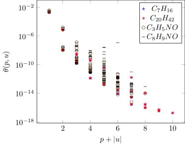
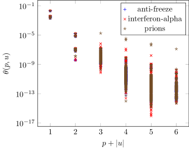
Figure 3: Benefit-cost ratios $\theta(p,u)$ versus the sum $p+|u|$ for several alkane, acrylamide, acetanilide and three proteins.

4.2 Numerical results for the approximation of energy

Now we consider the approximation of the energy of heptane by the approaches introduced in Section 3. To this end, we will shortly recall our notation of the energy approximations associated to the considered methods: $V_{p}^{HF}$ denotes the energy of the conventional HF method using a cc-pV$(n)$Z basis set with $n=p+3$ and $V_{p,k}^{BN}$ denotes the energy of the BOSSANOVA approach with basis set level $p$ and bond order $k$ according to equation (12). The energy of the multilevel BOSSANOVA approach for a general admissible index set $I$ is defined in (18) and is denoted by $V_{I}$. Here, inspired by the observations in Section 4.1, we first restrict ourselves to use the index sets $I=I^{TD}_{L,1}$ as defined in (19), which correspond to the regular sparse grids approach. Furthermore we consider the energy approximations $V_{I_{\alpha}}$ and $V_{\mathcal{I}_{\alpha}}$ according to the adaptive Algorithm 1 with equation (29) and the adaptive Algorithm 2 with equation (31), respectively.

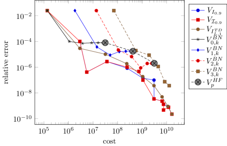
Figure 4: Relative error versus costs of different approximation methods for heptane, where we choose $V_{4}^{HF}$ as reference energy, i.e. the HF energy computed with the help of the cc-pV6Z basis set. Shown are for $p=0,1,2$ the energies $V_{p}^{HF}$ of the HF method, for $k=1,\ldots,6$ the energies $V_{p,k}^{BN}$ of the BOSSANOVA approach and for $L=1,\ldots,9$ the energies $V_{I^{TD}_{L,1}}$ of the the multilevel BOSSANOVA method. For the adaptive multilevel BOSSANOVA approach the energy of each step of Algorithm 1 and Algorithm 2 for $V_{{I}_{0.9}}$ and $V_{\mathcal{I}_{0.9}}$ are shown, respectively.

For the heptane example we choose the HF approach as the local electronic structure method. The results are given in Figure 4. We observe that the three multilevel BOSSANOVA approaches, i.e. $V_{I^{TD}_{L,1}}$, $V_{{I}_{0.9}}$ and $V_{\mathcal{I}_{0.9}}$, exhibit a substantially better convergence behavior than the HF and the standard BOSSANOVA method, i.e. than $V_{p}^{HF}$ and $V_{p,k}^{BN}$, respectively. Furthermore, we see that the adaptive variants, i.e. $V_{{I}_{0.9}}$ and $V_{\mathcal{I}_{0.9}}$, give almost the same results (for values with a relative error larger than 1.e-5 they are even exactly the same) and that both indeed show even a slightly better convergence behavior than the variant with a priori chosen index sets, i.e. $V_{I^{TD}_{L,1}}$.

Table 1: Comparison of the costs of the different methods to obtain a relative error less than a value of 1.e-5 for heptane. In addition the speed up factor for each method compared to the cost of the conventional HF method is given.

	rel. err.	cost	speed-up	parallel cost	parallel speed-up
$V_{2}^{HF}$	2.02e-6	6.7e+08	1.0	6.7e+8	1.0
$V^{BN}_{2,3}$	6.67e-6	3.7e+08	1.8	5.3e+7	12.7
$V_{I^{TD}_{4,1}}$	1.88e-6	2.4e+08	2.8	1.6e+7	42.9
$V_{{I}_{0.9}}$	2.75e-6	3.7e+07	18.1	2.9e+6	230.2
$V_{\mathcal{I}_{0.9}}$	2.75e-6	3.7e+07	18.1	2.9e+6	230.2

In addition, we compare in Table 1 the costs of all methods to obtain a specific accuracy. We obtain a speed-up factor of about $18$ for the cost of the two adaptive multilevel BOSSANOVA energies, i.e. $V_{{I}_{0.9}}$ and $V_{\mathcal{I}_{0.9}}$, compared to the energy value computed by the conventional HF method, i.e. $V_{2}^{HF}$. For the multilevel BOSSANOVA energy $V_{I^{TD}_{4,1}}$ we still get a speed up factor of about $2.8$ compared to the cost of $V_{2}^{HF}$. In the parallel cost model we obtain even a speed-up factor of about $230$ for $V_{{I}_{0.9}}$ and of about $43$ for $V_{I^{TD}_{4,1}}$. We thus see that, already for a small molecule like heptane, the gain of our new method is substantial. For larger molecules it should be even more profound.

Therefore, we apply our new adaptive approaches to the more complex molecules acetanilide ($C_{8}H_{9}NO$) and acrylamide ($C_{3}H_{5}NO$). Moreover, we varied the parameter $\alpha$ in a wider range of values. It turned out that values greater than $\alpha=0.75$ perform quite well. Thus, we considered $\alpha=0.9$ and $\alpha=0.99$ in the following. Our numerical results, given in Figure 5, show that the convergence behavior of both algorithms is similar. However, the results for acetanilide suggest that for more complex molecules the more general dimension-adaptive approximation approach according to (31) and Algorithm 2 is potentially superior compared to the more restrictive dimension-adaptive technique corresponding to Algorithm 1 and (29). Note that each approximation in form of equation (29) can be represented also in the form corresponding to (31), but this does not hold vice versa.

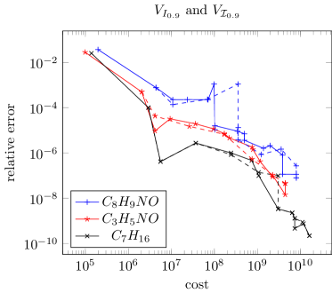
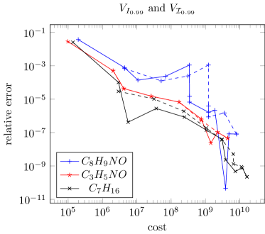
Figure 5: Relative error versus costs of Algorithm 1 and Algorithm 2. The solid lines correspond to the errors of the energies $V_{\mathcal{I}_{\alpha}}$ of Algorithm 2, while the dashed lines correspond to the errors of the energies $V_{{I}_{\alpha}}$ of Algorithm 1.

The larger the molecules are, the more profound the gain for our BOSSANOVA approach is compared to the conventional methods applied to the overall molecule. To show this we finally apply our new adaptive multilevel method to molecules which consist of so many atoms such that the conventional methods can no longer be applied in practice. To this end, as in Section 4.1, we will consider the anti-freeze protein, the interferon-$\alpha$ protein and the prion, where we now use the DFT method within our multilevel BOSSANOVA approach.

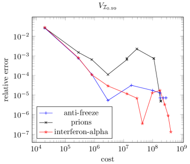
Figure 6: Relative error versus parallel costs of Algorithm 2, where we choose $V_{3,3}^{BN}$ as reference energy, i.e. the energy of the BOSSANOVA approach for basis set cc-pV6Z and bond order three.

The numerical results are given in Figure 6. There we choose as the reference energy to compute the relative error the BOSSANOVA energy $V_{3,3}^{BN}$, apply the parallel cost model and choose $\alpha=0.99$.

Altogether, the results of our numerical experiments suggest that indeed the adaptive multilevel BOSSANOVA approaches can be efficiently and successfully applied to larger molecules. Especially Algorithm 2 promises, due to its local refinement property, to enable systematic quasi-optimal approximations in a cost-efficient manner.

5 Concluding Remarks

In this article we presented the adaptive multilevel BOSSANOVA decomposition approach for the approximate ground state solution to the electronic Schrödinger equation for a given molecular system. Here, we followed the idea of sparse grids and the adaptive combination technique to obtain systematically quasi-optimal approximations, i.e. a specific truncation of the hierarchical series such that the total benefit is maximized for a fixed amount of costs.

We described and discussed an a priori truncation scheme and in particular two a posteriori dimension-adaptive algorithms for a seamless coupling of local computations whith a high level basis set where needed and low level basis sets where locally sufficient. We gave numerical results for small chain molecules, where we obtained substantial speed up factors compared to the cost of the conventional HF method. We furthermore presented numerical results for three large proteins. Here, the more general variant of the dimension-adaptive approach, which allows for local adaptivity, seems to be superior compared to the more restrictive variant, which does not allow for local adaptivity. Let us point out that our approach is trivial to parallelize since the evaluation of each fragment by an appropriate solver can be done independently, see e.g. [42].

In this article, for reasons of simplicity, we did not investigate the treatment of aromatic systems with delocalized electrons with ring structures in more detail. For such problems, there is surely room for further improvement of our algorithms. A simple modification of the conventional BOSSANOVA approach was already successfully applied to such systems in [35, 42]. The impact of the neglected long-range Coulomb energy on the accuracy of the method and techniques to recover this contribution were given elsewhere, see [42].

Note furthermore that the BOSSANOVA approach is not free of empirical parameters due to the necessity to saturate dangling bonds with hydrogen in the fragmentation process. But the typical bond lengths and angles of hydrogenated systems are well assessed by measurements.

6 Acknowledgments

The authors gratefully acknowledge the Hausdorff Center for Mathematics (HCM) and the Cooperative Research Centre (SFB 1060) at University of Bonn for the financial support. The authors also thank Frederik Heber (Numerical Analysis and Applied Mathematics, Saarland University) for useful discussions.

Appendix

Appendix A Modified energy terms $\widehat{V}^{G}_{p,u}$

Let $G$ be an connected interaction graph of a molecule. Then, according to the BOSSANOVA approach, the modified energy associated with a fragment $u$ is given by

$$\widehat{V}^{G}_{p,\{i_{1},\ldots,i_{k}\}}({X}_{\{i_{1},\ldots,i_{k}\}}):=\sum_{u\in\mathcal{C}(G)}V_{p}\left({X}_{i_{1}},\ldots,{X}_{i_{k}},R^{G}_{1}(u),\ldots,R^{G}_{h^{G}(u)}(u)\right),$$

where

$$\mathcal{C}((P,E)):=\bigl{\{}u\subseteq P\,:\,\text{ $(P_{u},E_{u})\subseteq(P,E)$ is connected and}\\ \text{for all $v\supsetneq u$ subgraph $(P_{v},E_{v})$ is not connected}\bigr{\}}.$$

Thus, it holds the relation

$$\widehat{V}_{p,A\cup B}^{G}(X_{A\cup B})=\widehat{V}_{p,A}^{G}(X_{A})+\widehat{V}_{p,A}^{G}(X_{A}),$$

for all $p\in\mathbb{N}$ and for all pairs of subsets $A,B\subseteq\{1,\ldots,M\}$ with disconnected induced subgraphs $G_{A},G_{B}\subseteq G$. Moreover, we can derive that the corresponding hierarchical surplus $w_{p,A\cup B}$ vanishes:

Lemma A.1.

Let $G=({P},{E})$ be an interaction graph. Let $A,B\subseteq{P}$, $A\cap B=\emptyset$ and let the subgraphs $G_{A}$ and $G_{B}$ induced by $A$ and $B$, respectively, be disconnected. Then

$$W^{G}_{p,A\cup B}({X}_{A\cup B})=0.$$

Proof.

We use induction: The base case can be easily seen for graphs $G=({P},{E})$ with sets $|{P}|\leq 2$. Let us assume that the statement holds for graphs $G=({P}^{\prime},{E}^{\prime})$ with $|{P}^{\prime}|\leq n$. Now let $G=({P},{E})$ with $|{P}|=n+1$. Note that from the recursive definition of $\widehat{V}^{G}_{p,a}$ it immediately follows that

$$\widehat{V}^{G}_{p,a}({X}_{a})=\sum_{b\subseteq a}w_{p,b}({X}_{b})$$

holds for all $a\subseteq{P}$. With $\widehat{V}^{G}_{p,A\cup B}(X_{A\cup B})=\widehat{V}^{G}_{p,A}(X_{A})+\widehat{V}^{G}_{p,B}(X_{B})$ and $W^{G}_{p,\emptyset}=0$, we then obtain

$$W^{G}_{p,A\cup B}({X}_{A\cup B}) =\widehat{V}^{G}_{A\cup B}({X}_{A\cup B})-\sum_{a\subseteq A,a\neq\emptyset}W^{G}_{p,a}({X}_{a})-\sum_{b\subseteq B,b\neq\emptyset}W^{G}_{p,b}({X}_{b})$$

$$\quad-\sum_{\begin{subarray}{c}a\subseteq A,b\subseteq B\\ a\neq\emptyset,b\neq\emptyset,|a\cup b|<|A\cup B|\end{subarray}}W^{G}_{p,a\cup b}({X}_{a\cup b})-W^{G}_{p,\emptyset}$$

$$=\widehat{V}^{G}_{p,A}({X}_{A})+\widehat{V}^{G}_{p,B}({X}_{B})$$

$$\quad-\sum_{a\subseteq A}W^{G}_{p,a}({X}_{a})-\sum_{b\subseteq B}W^{G}_{p,b}({X}_{b})-\sum_{\begin{subarray}{c}a\subseteq A,b\subseteq B\\ a\neq\emptyset,b\neq\emptyset,|a\cup b|<|A\cup B|\end{subarray}}W^{G}_{p,a\cup b}({X}_{a\cup b}).$$

Now, we apply the induction hypothesis to each $W^{G}_{p,A\cup B}$: $|a\cup b|<|A\cup B|\leq|{P}|=n+1$ and finally obtain

$$W^{G}_{p,A\cup B}({X}_{A\cup B}) =\widehat{V}^{G}_{p,A}({X}_{A})-\sum_{a\subseteq A}W^{G}_{p,a}({X}_{a})+\widehat{V}^{G}_{p,B}({X}_{B})-\sum_{b\subseteq B}W^{G}_{p,b}({X}_{b})$$

$$\quad-\sum_{\begin{subarray}{c}a\subseteq A,b\subseteq B\\ a\neq\emptyset,b\neq\emptyset,|a\cup b|<|A\cup B|\end{subarray}}W^{G}_{p,a\cup b}({X}_{a\cup b})$$

$$=-\sum_{\begin{subarray}{c}a\subseteq A,b\subseteq B\\ a\neq\emptyset,b\neq\emptyset,|a\cup b|<|A\cup B|\end{subarray}}W^{G}_{p,a\cup b}({X}_{a\cup b})=0.$$

∎

Appendix B Example (small linear molecule)

In the following, let us shortly give an example corresponding to a linear molecule of length three. Let $G=(\{1,2,3\},\{\{1,2\},\{2,3\}\}$. Then, from (14) and (8) it results for level $p=0$:

$$\omega_{0,\{1\}}(X_{\{1\}}) :=\widehat{V}_{0}(X_{\{1\}}),$$

$$\omega_{0,\{2\}}(X_{\{2\}}) :=\widehat{V}_{0}(X_{\{2\}}),$$

$$\omega_{0,\{3\}}(X_{\{3\}}) :=\widehat{V}_{0}(X_{\{3\}}),$$

$$\omega_{0,\{1,2\}}(X_{\{1,2\}}) :=\widehat{V}_{0}(X_{\{1,2\}})-(\omega_{0,\{1\}}(X_{\{1\}})+\omega_{0,\{2\}}(X_{\{2\}}))$$

$$\omega_{0,\{2,3\}}(X_{\{2,3\}}) :=\widehat{V}_{0}(X_{\{2,3\}})-(\omega_{0,\{2\}}(X_{\{2\}})+\omega_{0,\{3\}}(X_{\{3\}})),$$

$$\omega_{0,\{1,2,3\}}(X_{\{1,2,3\}}) :=\widehat{V}_{0}(X_{\{1,2,3\}})-(\omega_{0,\{2,3\}}(X_{\{2,3\}})+\omega_{0,\{1,2\}}(X_{\{1,2\}})+\omega_{0,\{1\}}+\omega_{0,\{2\}}+\omega_{0,\{3\}}).$$

For level $p=1$ we obtain:

$$\omega_{1,\{1\}}(X_{\{1\}}):=\widehat{V}_{1}(X_{\{1\}}) -\omega_{0,\{1\}}(X_{\{1\}}),$$

$$\omega_{1,\{2\}}(X_{\{2\}}):=\widehat{V}_{1}(X_{\{2\}}) -\omega_{0,\{2\}}(X_{\{2\}}),$$

$$\omega_{1,\{3\}}(X_{\{3\}}):=\widehat{V}_{1}(X_{\{3\}}) -\omega_{0,\{3\}}(X_{\{3\}}),$$

$$\omega_{1,\{1,2\}}(X_{\{1,2\}}):=\widehat{V}_{1}(X_{\{1,2\}}) -(\omega_{1,\{1\}}(X_{\{1\}})+\omega_{1,\{2\}}(X_{\{2\}}))-(\omega_{1,\{1\}}(X_{\{1\}})+\omega_{1,\{2\}}(X_{\{2\}}))$$

$$\omega_{1,\{2,3\}}(X_{\{2,3\}}):=\widehat{V}_{1}(X_{\{2,3\}}) -(\omega_{1,\{2\}}(X_{\{2\}})+\omega_{1,\{3\}}(X_{\{3\}}))-(\omega_{0,\{2\}}(X_{\{2\}})+\omega_{0,\{3\}}(X_{\{3\}})),$$

$$\omega_{0,\{1,2,3\}}(X_{\{1,2,3\}}):=\widehat{V}_{1}(X_{\{1,2,3\}}) -(\omega_{1,\{2,3\}}(X_{\{2,3\}})+\omega_{1,\{1,2\}}(X_{\{1,2\}})+\omega_{1,\{1\}}+\omega_{1,\{2\}})$$

$$-(\omega_{0,\{2,3\}}(X_{\{2,3\}})+\omega_{0,\{1,2\}}(X_{\{1,2\}})+\omega_{0,\{1\}}+\omega_{0,\{2\}}).$$

Note here that the induced subgraph $G_{\{1,3\}}$ is not connected. Hence, the contributions $\omega_{p,\{1,3\}}$ are zero for all $p\in\mathbb{N}$.

References

- [1] G. Abell. Empirical chemical pseudopotential theory of molecular and metallic bonding. Physical Review B, 31(10):6184–6196, 1985.
- [2] L. Ambrosio, A. Figalli, G. Friesecke, J. Giannoulis, and T. Paul. Semiclassical limit of quantum dynamics with rough potentials and well-posedness of transport equations with measure initial data. Communications on Pure and Applied Mathematics, 64(9):1199–1242, 2011.
- [3] A. Amovilli, I. Cacelli, S. Campanile, and G. Prampolini. Calculation of the intermolecular energy of large molecules by a fragmentation scheme: Application to the 4-n-pentyl-4-cyanobiphenyl (5CB) dimer. Journal of Chemical Physics, 117:3003–3012, 2002.
- [4] J.-M. André. The Nobel Prize in chemistry 2013. Chemistry International, 36(2):2–7, 2014.
- [5] D. Bates, J. Smith, T. Janowski, and G. Tschumper. Development of a 3-body: many-body integrated fragmentation method for weakly bound clusters and application to water clusters () n = 3-10, 16, 17. The Journal of Chemical Physics, 135(4):044123, 2011.
- [6] G. Beran. Approximating quantum many-body intermolecular interactions in molecular clusters using classical polarizable force fields. The Journal of Chemical Physics, 130(16):164115, 2009.
- [7] D. Bowler and T. Miyazaki. O(N) methods in electronic structure calculations. Reports on Progress in Physics, 75(3):036503, 2012.
- [8] D. Brenner. A second-generation reactive bond order (REBO) potential energy expression for hydrocarbons. Journal of Physics: Condensed Matter, 14:783–802, 2002.
- [9] C. Le Bris. Computational chemistry from the perspective of numerical analysis. Acta Numerica, 14:363–444, 2005.
- [10] H-J. Bungartz and M. Griebel. Sparse grids. Acta Numerica, 13:147–269, 2004.
- [11] H.-J. Bungartz, M. Griebel, D. Röschke, and C. Zenger. A proof of convergence for the combination technique for the Laplace equation using tools of symbolic computation. Mathematics and Computers in Simulation, 42:595–605, 1996.
- [12] P. Bygrave, N. Allan, and F. Manby. The embedded many-body expansion for energetics of molecular crystals. The Journal of Chemical Physics, 137(16):164102, 2012.
- [13] E. Cancès, C. Le Bris, and P-L. Lions. Molecular simulation and related topics: some open mathematical problems. Nonlinearity, 21(9):T165–T176, 2008.
- [14] E. Cancès, M. Defranceschi, W. Kutzelnigg, C. Le Bris, and Y. Maday. Computational Quantum Chemistry: A primer. Handbook of Numerical Analysis, 10:3–270, 2003.
- [15] S. Carter, S. Culik, and J. Bowman. Vibrational self-consistent field method for many-mode systems: A new approach and application to the vibrations of CO adsorbed on Cu (100). The Journal of Chemical Physics, 107(24):10458–10469, 1997.
- [16] M. Collins and V. Deev. Accuracy and efficiency of electronic energies from systematic molecular fragmentation. Journal of Chemical Physics, 125:104104, 2006.
- [17] E. Dahlke and D. Truhlar. Electrostatically embedded many-body correlation energy, with applications to the calculation of accurate second-order Møller-Plesset perturbation theory energies for large water clusters. Journal of Chemical Theory and Computation, 3(4):1342–1348, 2007.
- [18] M. Daw and M. Baskes. Embedded-atom method: Derivation and application to impurities, surfaces and other defects in metals. Physical Review B, 29(12):6443–6453, 1984.
- [19] V. Deev and M. A. Collins. Approximate ab initio energies by systematic molecular fragmentation. Journal of Chemical Physics, 122(15):154102, 2005.
- [20] N. DeYonker, T. Cundari, and A. Wilson. The correlation consistent composite approach (ccCA): An alternative to the Gaussian-n methods. The Journal of Chemical Physics, 124(11):114104, 2006.
- [21] T. Dunning. Gaussian basis sets for use in correlated molecular calculations. I. The atoms boron through neon and hydrogen. The Journal of Chemical Physics, 90(2):1007–1023, 1989.
- [22] P. Elliott, K. Burke, M. Cohen, and A. Wasserman. Partition density-functional theory. Physical Review A, 82(2):024501, 2010.
- [23] P. Fast, M. Sánchez, and D. Truhlar. Infinite basis limits in electronic structure theory. The Journal of Chemical Physics, 111(7):2921–2926, 1999.
- [24] D. Feller. The use of systematic sequences of wave functions for estimating the complete basis set, full configuration interaction limit in water. The Journal of Chemical Physics, 98(9):7059–7071, 1993.
- [25] M. Field, P. Bash, and M. Karplus. A combined quantum mechanical and molecular mechanical potential for molecular dynamics simulations. Journal of Computational Chemistry, 11(6):700–733, 1990.
- [26] G. Friesecke. The multiconfiguration equations for atoms and molecules: charge quantization and existence of solutions. Archive for Rational Mechanics and Analysis, 169(1):35–71, 2003.
- [27] T. Gerstner and M. Griebel. Numerical integration using sparse grids. Numer. Algorithms, 18:209–232, 1998.
- [28] T. Gerstner and M. Griebel. Dimension–adaptive tensor–product quadrature. Computing, 71(1):65–87, 2003.
- [29] S. Goedecker. Linear scaling electronic structure methods. Reviews of Modern Physics, 71(4):1085–1123, 1999.
- [30] U. Góra, R. Podeszwa, W. Cencek, and K. Szalewicz. Interaction energies of large clusters from many-body expansion. The Journal of Chemical Physics, 135(22):224102, 2011.
- [31] M. Gordon, D. Fedorov, S. Pruitt, and L. Slipchenko. Fragmentation methods: a route to accurate calculations on large systems. Chemical Reviews, 112(1):632–672, 2012.
- [32] N. Gresh, P. Claverie, and A. Pullman. Theoretical studies of molecular conformation. Derivation of an additive procedure for the computation of intramolecular interaction energies. Comparison with ab-initio SCF computations. Theoretica Chimica Acta, 66:1–20, 1984.
- [33] M. Griebel and J. Hamaekers. Sparse grids for the Schrödinger equation. ESAIM: Mathematical Modelling and Numerical Analysis, 41(02):215–247, 2007.
- [34] M. Griebel and J. Hamaekers. Tensor product multiscale many-particle spaces with finite-order weights for the electronic Schrödinger equation. Zeitschrift für Physikalische Chemie, 224(3-4):527–543, 2010.
- [35] M. Griebel, J. Hamaekers, and F. Heber. A bond order dissection ANOVA approach for efficient electronic structure calculations. In Extraction of Quantifiable Information from Complex Systems, pages 211–235. Springer, 2014.
- [36] M. Griebel and H. Harbrecht. On the convergence of the combination technique. In Sparse grids and Applications, volume 97 of Lecture Notes in Computational Science and Engineering, pages 55–74. Springer, 2014.
- [37] M. Griebel, S. Knapek, and G. Zumbusch. Numerical Simulation in Molecular Dynamics – Numerics, Algorithms, Parallelization, Applications. Springer-Verlag, Heidelberg, 2007.
- [38] A. Halkier, T. Helgaker, P. Jørgensen, W. Klopper, H. Koch, J. Olsen, and A. Wilson. Basis-set convergence in correlated calculations on Ne, N2, and H2O. Chemical Physics Letters, 286(3):243–252, 1998.
- [39] J. Hamaekers. Sparse Grids for the Electronic Schrödinger Equation: Construction and Application of Sparse Tensor Product Multiscale Many-Particle Spaces with Finite-Order Weights for Schrödinger’s Equation. Südwestdeutscher Verlag für Hochschulschriften, Saarbrücken, 2010.
- [40] M. Y. Hayes, B. Li, and H. Rabitz. Estimation of molecular properties by high-dimensional model representation. Journal of Physical Chemistry, 110:264–272, 2006.
- [41] F. Heber. MoleCuilder - a molecular builder. https://trac.ins.uni-bonn.de/projects/molecuilder.
- [42] F. Heber. Ein systematischer, linear skalierender Fragmentansatz für das Elektronenstukturproblem. PhD thesis, Intitut für Numerische Simulation, Rheinische Friedrich-Wilhelms-Universität Bonn, 2014.
- [43] T. Helgaker, W. Klopper, H. Koch, and J. Noga. Basis-set convergence of correlated calculations on water. The Journal of Chemical Physics, 106(23):9639–9646, 1997.
- [44] C. Huang, M. Pavone, and E. Carter. Quantum mechanical embedding theory based on a unique embedding potential. The Journal of Chemical Physics, 134(15):154110, 2011.
- [45] C. Janssen, I. Nielsen, M. Leininger, E. Valeev, and E. Seidl. The Massively Parallel Quantum Chemistry Program (MPQC). Sandia National Laboratories, Livermore, CA, USA, 2004.
- [46] F. Jensen. Estimating the Hartree-Fock limit from finite basis set calculations. Theoretical Chemistry Accounts, 113(5):267–273, 2005.
- [47] F. Jensen. Introduction to Computational Chemistry. John Wiley & Sons, 2013.
- [48] P. Jurečka, J. Šponer, J. Černỳ, and P. Hobza. Benchmark database of accurate (MP2 and CCSD (T) complete basis set limit) interaction energies of small model complexes, DNA base pairs, and amino acid pairs. Physical Chemistry Chemical Physics, 8(17):1985–1993, 2006.
- [49] K. Kitaura, E. Ikeo, T. Asada, T. Nakano, and M. Uebayasi. Fragment molecular orbital method: an approximate computational method for large molecules. Chemical Physics Letters, 313:701–706, 1999.
- [50] W. Kohn. Density functional and density matrix method scaling linearly with the number of atoms. Physical Review Letters, 76(17):3168, 1996.
- [51] Y. Komeiji, T. Nakano, K. Fukuzawa, Y. Ueno, Y. Inadomi, T. Nemoto, M. Uebayasi, D. Fedorov, and K. Kitaura. Fragment molecular orbital method: application to molecular dynamics simulation, ab initio FMO-MD. Chemical Physics Letters, 372(3):342–347, 2003.
- [52] H.-C. Kreusler and H. Yserentant. The mixed regularity of electronic wave functions in fractional order and weighted Sobolev spaces. Numerische Mathematik, 121(4):781–802, 2012.
- [53] K. Lao, K.-Y. Liu, R. Richard, and J. Herbert. Understanding the many-body expansion for large systems. II. Accuracy considerations. The Journal of Chemical Physics, 144(16):164105, 2016.
- [54] C. Lubich. From Quantum to Classical Molecular Dynamics: Reduced Models and Numerical Analysis. European Mathematical Society, 2008.
- [55] J. Martin. Ab initio thermochemistry beyond chemical accuracy for first-and second-row compounds. In Energetics of Stable Molecules and Reactive Intermediates, pages 373–415. Springer, 1999.
- [56] D. Marx and J. Hutter. Ab initio molecular dynamics: Theory and implementation. In Modern Methods and Algorithms of Quantum Chemistry, volume 1 of NIC Series, pages 301–440. Forschungszentrum Juelich, Deutschland, 2000.
- [57] F. Maseras and K. Morokuma. IMOMM - a new integrated ab-initio plus molecular mechanics geometry optimization scheme of equilibrium structures and transition-states. Journal of Computational Chemistry, 16(9):1170–1179, 1995.
- [58] N. Mayhall and K. Raghavachari. Molecules-in-molecules: An extrapolated fragment-based approach for accurate calculations on large molecules and materials. Journal of Chemical Theory and Computation, 7(5):1336–1343, 2011.
- [59] A. Nakano, M. Bachlechner, R. Kalia, E. Lidorikis, P. Vashishta, G. Voyiadjis, T. Campbell, S. Ogata, and F. Shimojo. Multiscale simulation of nanosystems. Computing in Science & Engineering, 3(4):56–66, 2001.
- [60] F. Nobile, L. Tamellini, and R. Tempone. Convergence of quasi-optimal sparse-grid approximation of Hilbert-space-valued functions: application to random elliptic PDEs. Numerische Mathematik, pages 1–46, 2015.
- [61] W. Ohlinger, P. Klunzinger, B. Deppmeier, and W. Hehre. Efficient calculation of heats of formation. The Journal of Physical Chemistry A, 113(10):2165–2175, 2009.
- [62] K. Peterson and T. Dunning. Accurate correlation consistent basis sets for molecular core–valence correlation effects: The second row atoms Al–Ar, and the first row atoms B–Ne revisited. The Journal of Chemical Physics, 117(23):10548–10560, 2002.
- [63] K. Peterson, D. Woon, and T. Dunning. Benchmark calculations with correlated molecular wave functions. IV. the classical barrier height of the reaction. The Journal of Chemical Physics, 100(10):7410–7415, 1994.
- [64] M. Praprotnik, L. Site, and K. Kremer. Multiscale simulation of soft matter: From scale bridging to adaptive resolution. Annu. Rev. Phys. Chem., 59:545–571, 2008.
- [65] E. Prodan and W. Kohn. Nearsightedness of electronic matter. Proceedings of the National Academy of Sciences of the United States of America, 102(33):11635–11638, 2005.
- [66] R. Richard and J. Herbert. A generalized many-body expansion and a unified view of fragment-based methods in electronic structure theory. The Journal of Chemical Physics, 137(6):064113, 2012.
- [67] R. Richard, K. Lao, and J. Herbert. Understanding the many-body expansion for large systems. I. Precision considerations. The Journal of Chemical Physics, 141(1):014108, 2014.
- [68] R. Schneider. Analysis of the projected coupled cluster method in electronic structure calculation. Numerische Mathematik, 113(3):433–471, 2009.
- [69] H. Senn and W. Thiel. QM/MM methods for biomolecular systems. Angewandte Chemie International Edition, 48(7):1198–1229, 2009.
- [70] F. Shimojo, R. Kalia, A. Nakano, and P. Vashishta. Divide-and-conquer density functional theory on hierarchical real-space grids: Parallel implementation and applications. Physical Review B, 77(8):085103, 2008.
- [71] C.-K. Skylaris, P. Haynes, A. Mostofi, and M. Payne. Introducing ONETEP: Linear-scaling density functional simulations on parallel computers. Journal of Chemical Physics, 122(8):84119, 2005.
- [72] J. Tersoff. Modeling solid-state chemistry: Interatomic potentials for multicomponent systems. Physical Review B, 39:5566–5568, 1989.
- [73] D. Truhlar. Basis-set extrapolation. Chemical Physics Letters, 294(1):45–48, 1998.
- [74] G. Tschumper. Multicentered integrated QM:QM methods for weakly bound clusters: An efficient and accurate 2-body: many-body treatment of hydrogen bonding and van der Waals interactions. Chemical Physics Letters, 427(1):185–191, 2006.
- [75] T. Vreven and K. Morokuma. On the application of the IMOMO (integrated molecular orbital + molecular orbital) method. Journal of Computational Chemistry, 21(16):1419–1432, 2000.
- [76] L.-W. Wang. Divide-and-conquer quantum mechanical material simulations with exascale supercomputers. National Science Review, 1(4):604–617, 2014.
- [77] S. Weno, K. Nanda, Y. Huang, and G. Beran. Practical quantum mechanics-based fragment methods for predicting molecular crystal properties. Physical Chemistry Chemical Physics, 14(21):7578–7590, 2012.
- [78] A. Wilson, T. van Mourik, and T. Dunning. Gaussian basis sets for use in correlated molecular calculations. VI. Sextuple zeta correlation consistent basis sets for boron through neon. Journal of Molecular Structure: THEOCHEM, 388:339–349, 1996.
- [79] W. Yang and T.-S. Lee. A density-matrix divide-and-conquer approach for electronic structure calculations of large molecules. The Journal of Chemical Physics, 103(13):5674–5678, 1995.
- [80] H. Yserentant. Regularity, complexity, and approximability of electronic wavefunctions. In Extraction of Quantifiable Information from Complex Systems, pages 413–428. Springer, 2014.
- [81] Harry Yserentant. Regularity and Approximability of Electronic Wave Functions. Springer, 2010.
- [82] A. Zeiser. Wavelet approximation in weighted Sobolev spaces of mixed order with applications to the electronic Schrödinger equation. Constructive Approximation, 35(3):293–322, 2012.
- [83] J. Řezáč and D. Salahub. Multilevel fragment-based approach (MFBA): a novel hybrid computational method for the study of large molecules. Journal of Chemical Theory and Computation, 6(1):91–99, 2009.