Low-temperature evolution of the spectral weight of a spin-up carrier moving in a ferromagnetic background

Abstract

We derive the lowest-temperature correction to the self-energy of a spin-up particle injected in a ferromagnetic background. The background is modeled with both Heisenberg and Ising Hamiltonians so that differences due to gapless vs. gapped magnons can be understood. Beside the expected thermal broadening of the quasiparticle peak as it becomes a resonance inside a continuum, we also find that spectral weight is transferred to regions lying outside this continuum. We explain the origin of this spectral weight transfer and its low-temperature evolution.

I Introduction

The problem of understanding the behavior of a carrier doped into a magnetically ordered insulator is relevant for the study of many materials. Multiple variations are possible: the carrier may enter into the same band that gives rise to the magnetic order, or, as if often the case, may be hosted in a different band. The background might have antiferromagnetic (AFM) order (parent cupratescuprates being the most famous example), or ferromagnetic (FM) order (in ferromagnetic chalcogenides like EuO) or more complicated forms of magnetic order, such as FM layers that are layered antiferomagnetically in manganite perovskites,Ramirez (1997); Nolting et al. (2001) zig-zag order in iridates,iridates etc. Finally, the magnetic order may be present in the undoped compound (all examples listed above) or may arise as a result of doping, like in diluted magnetic semiconductors such as Ga_1-xMn_xAs,GaMnAs or heavy fermion materials like CeSi_x.Lee et al. (1987); Nolting et al. (2001) Understanding the properties of such materials has direct technological implications since many of them are candidates for new spintronic and magnetoelectric devices.Wolf et al. (2001)

The degree of difficulty in solving such problems varies widely. The most difficult problems are those with AFM backgrounds, because of their inherent complexity due to the presence of quantum spin fluctuations – this explains why what happens when one hole is doped into an AFM cuprate layer is still being debated.Bayo

In contrast, FM backgrounds are exactly solvable, especially at $T=0$. On the other hand, unlike in the AFM case, here the spectrum of the carrier has a striking dependence on its spin direction. If the carrier is injected with its spin oriented parallel to the local moments, no spin-flip excitations are possible and the carrier moves freely. Its spectrum is identical to that of a free carrier up to an energy shift due to the $zz$ component of the magnetic exchange. If the carrier is injected with its spin anti-parallel to the local moments, the formation of a dressed quasi-particle, a so-called spin-polaron, is possible. This is a state where the carrier continuously emits and re-absorbs a magnon while flipping its spin from up to down, in a coherent fashion. There are also states where the carrier has spin-up and the magnon is present (as required by conservation of the $z$-component of the total spin) but not bound to the carrier, giving rise to a continuum of incoherent states distinct from the spin-polaron discrete state.

The fact that only one magnon can be emitted by a spin-down carrier injected in a $T=0$ FM background (assuming the carrier has spin-$\frac{1}{2}$, which we do here) explains why there exists an exactly solvable solution for such problems. The solution was first given by Shastry and MattisShastry and Mattis (1981) and has recently been generalized to more complex lattices.Berciu and Sawatzky (2009) Furthermore, exact analytical derivations of the eigenstates and eigenenergies were recently presented by Henning et al.Henning et al. (2012) and by Nakano et al. NAKANO et al. (2012) for Hamiltonians describing such problems.

As far as we know, the only other exact solution for a generalization of this simplest case is for two carriers injected in the FM background,Mirko because the number of possible additional magnons is still very small, resulting in a solvable few-body problem. Dealing with finite carrier concentrations which can induce finite concentrations of magnons requires the use of approximations,Nolting et al. (1997) except in the very trivial case when all carriers have spin-up.

Here we consider another and in real life more interesting generalization, namely that of studying the spectrum of a spin-up carrier injected in a FM background at finite $T$. An exact solution is no longer possible since one needs to consider states with arbitrary numbers of magnons when performing temperature averages. A natural approach for low-$T$ is to consider states with a small number of magnons; this is what we do here. As a result, the solution we propose becomes asymptotically exact in the limit of very low temperatures, where “low” means well-below the Curie critical temperature $T_{C}$ of the FM background.

As mentioned, a spin-up carrier has a very simple spectrum at $T=0$, mirroring that of the free carrier, with a single eigenstate for a given momentum. At $T\neq 0$ thermally activated magnons are present in the system and the carrier can now flip its spin by absorbing one of them. Interaction with even one such magnon takes the problem in the Hilbert subspace appropriate for the $T=0$ spin-down carrier, which has a very different spectrum. As a result, we expect that spectral weight is transferred from the spin-up quasiparticle peak to energies in the spectrum of the spin-polaron, as $T$ increases. How exactly does this occur at very low $T$, and what happens to the infinitely-lived discrete state that was the only feature in the spectrum at $T=0$, is the topic of this work.

Furthermore, we consider two types of exchange between the local moments, namely Heisenberg exchange and Ising exchange (in both cases, the characteristic energy scale is $J$). For the latter the magnon spectrum is gapped, whereas for the former the magnon spectrum is gapless. This allows us to contrast the two cases to understand the relevance of the magnon’s spectrum on the evolution of the up carrier’s spectral function with $T$.

Finite temperature studies have been previously carried out by Nolting et al.Nolting et al. (2001) for the Kondo lattice model (KLM), which is also often referred to as the s-f model. This model accounts for the kinetic energy of the carrier as described by a tight-binding model with an energy scale $t$, and for the exchange between the local moments and the carrier, described by a Heisenberg exchange with a coupling $J_{0}$. Unlike the models we consider, KLM does not include the exchange $J$ between local moments; this is one key difference between our work and theirs. The second is the approach employed. While, as mentioned, we use a low-$T$ expansion to calculate the propagator, Nolting et al. proposed an ansatz for the self-energy chosen so as to reproduce asymptotic limits where an exact solution is available, specifically the $T=0$ solution mentioned above and the case of finite $T$ but zero bandwidth, $t=0$.Nolting and Matlak (1984) (This approach was later generalized to finite carrier concentrations as well.Nolting et al. (1997)) Their ansatz for the self-energy contains several free parameters which are fixed by fitting them to a finite number of exactly calculated spectral moments. The temperature dependence is contained implicitly in the magnetization which enters the self-energy as an external parameter. In the limit of very low-$T$ we consider here, the average local moment is essentially unchanged from its $T=0$ value, so the effects we uncover are basically absent in the ansatz of Nolting et al. In other words, besides studying different Hamiltonians by very different means, our studies also focus on very different regimes: very low $T$, in our work, vs. medium and high $T$ in Ref. Nolting and Matlak, 1984. Needless to say, in the absence of an exact solution it is likely that a collection of approximations valid in different regimes will be needed in order to fully understand this problem.

The article is organized as follows: in Section II we introduce our models and in Section III we derive the lowest-T self-energy correction. Section IV presents our results and Section V contains our conclusions.

II Models

We consider a single spin-${1\over 2}$ charge carrier which propagates on a hypercubic lattice with periodic boundary conditions after $N_{i}$ sites in the direction $i=1,d$; the total number of sites is $N=\prod_{i=1}^{d}N_{i}$. Our results are for $d=2$ and $d=3$. Of course, long-range FM order at finite-T only exists in $d=3$. However, we also consider anisotropic layered compounds, like the manganites, which have 2D FM layers whose finite-T long-range order is stabilized by weak inter-layer coupling, but where one can assume that at very low-$T$ the intra-layer carrier dynamics determine its properties. In principle, similar arguments can be employed to study $d=1$ chains with FM order at finite-$T$ maintained by their immersion in 3D lattices, but complications due to formation of magnetic domains would still need to be dealt with.

The carrier is an electron in an otherwise empty band or a hole in an otherwise full band, described by a tight binding model with nearest neighbor (nn) hopping:

$$\hat{T}=\sum_{\mathbf{k},\sigma}\epsilon(\mathbf{k})c^{\dagger}_{\mathbf{k},\sigma}c_{\mathbf{k},\sigma},$$ (1)

with $\epsilon(\mathbf{k})=-2t\sum_{i=1}^{d}\cos k_{i}$ for lattice constant $a=1$. $c_{\mathbf{k},\sigma}^{\dagger}$ creates a carrier with momentum $\mathbf{k}$ and spin $\sigma$.

The local magnetic moments are described by either a Heisenberg or an Ising interaction:

$$\hat{H}_{S}=-J\sum_{\langle i,j\rangle}\left(\mathbf{S}_{i}\cdot\mathbf{S}_{j}-S^{2}\right)$$ (2)

for Heisenberg exchange, while for Ising exchange:

$$\hat{H}_{I}=-J\sum_{\langle i,j\rangle}\left(S^{z}_{i}S^{z}_{j}-S^{2}\right),$$ (3)

where $\mathbf{S}_{i}$ is the spin-$S$ moment located at site $\mathbf{R}_{i}$ and only nn exchange is included in both models. We represent local moments with a double arrow, eg. $\Uparrow$, while the carrier spin is represented by a single arrow, eg. $\uparrow$.

For both these models the undoped ground state is $|{\rm FM}\rangle=\mid\Uparrow,\Uparrow,\dots\rangle$ and has zero energy. The only excited states of interest will be the single magnon states:

$$|\Phi(\mathbf{q})\rangle=\frac{S^{-}_{\mathbf{q}}}{\sqrt{2S}}|{\rm FM}\rangle=\sum_{j}\frac{\mathrm{e}^{i\mathbf{q}\mathbf{R}_{j}}}{\sqrt{2SN}}S_{j}^{-}|{\rm FM}\rangle.$$ (4)

Here $S^{\pm}_{i}=S^{x}_{i}\pm iS^{y}_{i}$ are the raising $(+)$ and lowering $(-)$ operators. The key difference between the Heisenberg and Ising interactions is the dispersion of the single magnon states. For the Heisenberg model this is $\Omega_{\mathbf{q}}=4JS\sum_{i=1}^{d}\sin^{2}(q_{i}/2)$, whereas for the Ising model the magnons are dispersionless, $\Omega_{\mathbf{q}}=\Omega=2dJS$.

The interaction between the carrier and the local moments is also a Heisenberg exchange:

$$\hat{H}_{\text{exc}}=J_{0}\sum_{j}\mathbf{s}_{j}\cdot\mathbf{S}_{j},$$ (5)

where $\mathbf{s}_{i}=\sum_{\alpha,\beta}c_{i,\alpha}^{\dagger}\frac{\mathbf{\sigma}_{\alpha,\beta}}{2}c_{i,\beta}$ is the carrier spin operator and $\mathbf{\sigma}$ are the Pauli matrices. The coupling $J_{0}$ can be either FM or AFM; we will consider both cases.

It is convenient to split $\hat{H}_{\text{exc}}=\hat{H}_{\text{exc}}^{z}+\hat{H}_{\text{exc}}^{x,y}$, where $\hat{H}_{\text{exc}}^{z}=J_{0}/2\sum_{j}\left(c_{j,\uparrow}^{\dagger}c_{j,\uparrow}-c_{j,\downarrow}^{\dagger}c_{j,\downarrow}\right)S^{z}_{j}$ and $\hat{H}_{\text{exc}}^{x,y}=J_{0}/2\sum_{j}\left(c_{j,\uparrow}^{\dagger}c_{j,\downarrow}S^{-}_{j}+c_{j,\downarrow}^{\dagger}c_{j,\uparrow}S^{+}_{j}\right).$ The first term causes an energy shift $\pm J_{0}S/2$. The second term is responsible for spin-flip processes, where the carrier flips its spin by absorbing or emitting a magnon.

The total Hamiltonian is:

$$\hat{H}=\hat{T}+\hat{H}_{\text{S/I}}+\hat{H}_{\text{exc}}.$$ (6)

Due to translational invariance, the total momentum is conserved. Furthermore, the $z-$component $S_{\text{tot}}^{z}$ of the total spin (the sum of the carrier spin and lattice spins), is also conserved. Therefore, eigenstates $\hat{H}|\psi^{(m)}_{\alpha}(\mathbf{k})\rangle=E_{\alpha}^{(m)}(\mathbf{k})|\psi^{(m)}_{\alpha}(\mathbf{k})\rangle$ are indexed by the total momentum of the system, $\mathbf{k}$, by the number $m$ of magnons when the carrier has spin-up so that $S_{\text{tot}}^{z}=NS+\frac{1}{2}-m$, and by $\alpha$ which comprises all the other quantum numbers.

III Formalism

We want to calculate the low-T expression of Zubarev’s double-time retarded propagatorzubarev for a spin-up carrier:

$$G_{\uparrow}(\mathbf{k},\tau)=-\frac{i}{Z}\Theta(\tau)\operatorname{Tr}[\mathrm{e}^{-\beta\hat{H}}c_{\mathbf{k},\uparrow}(\tau)c_{\mathbf{k},\uparrow}^{\dagger}(0)],$$ (7)

but in a canonical (not grand-canonical) ensemble, assuming that the carrier is injected in the otherwise undoped FM. As a result, the trace is over the eigenstates of $\hat{H}_{\text{S/I}}$ (in the absence of carriers, $\hat{H}\equiv\hat{H}_{\text{S/I}}$). $\Theta(\tau)$ is the Heaviside function, $Z=\operatorname{Tr}[\mathrm{e}^{-\beta\hat{H}_{\text{S/I}}}]$ is the partition function for the undoped FM, and $c_{\mathbf{k},\uparrow}(\tau)=\mathrm{e}^{i\tau\hat{H}}c_{\mathbf{k},\uparrow}\mathrm{e}^{-i\tau\hat{H}}$ is the carrier annihilation operator in the Heisenberg picture. In the frequency domain we have:

$$G_{\uparrow}(\mathbf{k},\omega)=\int_{-\infty}^{\infty}d\tau e^{i\omega\tau}G_{\uparrow}(\mathbf{k},\tau).$$

At $T=0$, the trace reduces to a trivial expectation value over $|{\rm FM}\rangle$, and we find:Shastry and Mattis (1981)

$$G^{(0)}_{\uparrow}(\mathbf{k},\omega)=\langle{\rm FM}|c_{\mathbf{k},\uparrow}\hat{G}(\omega)c^{\dagger}_{\mathbf{k},\uparrow}|{\rm FM}\rangle=\frac{1}{\omega-E_{\uparrow}(\mathbf{k})+i\eta}.$$

Here $\hat{G}(\omega)=[\omega-\hat{H}+i\eta]^{-1}$ is the resolvent of $\hat{H}$ and $\eta$ is a small, positive number (we set $\hbar=1$). Physically, $1/\eta$ sets the carrier lifetime. The eigenenergy is $E_{\uparrow}(\mathbf{k})=\epsilon(\mathbf{k})+J_{0}\frac{S}{2}$ for both the Heisenberg and Ising models. As discussed, this shows that at $T=0$ a spin-up carrier propagates freely and acquires an energy shift from $\hat{H}_{\text{exc}}^{z}$.

At finite temperature, we expect to find:

$$G(\mathbf{k},\omega)=\frac{1}{\omega-E_{\uparrow}(\mathbf{k})-\Sigma(\mathbf{k},\omega)+i\eta}$$

$$=G^{(0)}_{\uparrow}(\mathbf{k},\omega)+G^{(0)}_{\uparrow}(\mathbf{k},\omega)\Sigma(\mathbf{k},\omega)G^{(0)}_{\uparrow}(\mathbf{k},\omega)+\dots$$ (8)

Strictly speaking, the energy shift $J_{0}\frac{S}{2}$ is part of the self-energy, however it is convenient to separate it as we do here so that $\Sigma(\mathbf{k},\omega)$ contains only the finite-$T$ terms.

Since we are interested in the lowest-$T$ contribution to $\Sigma(\mathbf{k},\omega)$, we consider only the first two terms of Eq. (7):

$$G_{\uparrow}(\mathbf{k},\omega)=\frac{G_{\uparrow}^{(0)}(\mathbf{k},\omega)+\sum_{\mathbf{q}}\mathrm{e}^{-\beta\Omega_{\mathbf{q}}}G_{\uparrow}^{(1)}(\mathbf{k},\mathbf{q},\mathbf{q},\omega)+\dots}{1+\sum_{\mathbf{q}}\mathrm{e}^{-\beta\Omega_{\mathbf{q}}}+\dots},$$ (9)

where we define the new propagators $G_{\uparrow}^{(1)}(\mathbf{k},\mathbf{q},\mathbf{q}^{\prime},\omega)=-i\int_{0}^{\infty}\mathrm{d}\tau\,\mathrm{e}^{i\omega\tau}\langle\Phi(\mathbf{q}^{\prime})|c_{\mathbf{k},\uparrow}(\tau)c_{\mathbf{k+q^{\prime}-q},\uparrow}^{\dagger}|\Phi(\mathbf{q})\rangle.$ Only diagonal $\mathbf{q^{\prime}}=\mathbf{q}$ terms contribute to the trace. After carrying out the Fourier transform we find $G_{\uparrow}^{(1)}(\mathbf{k},\mathbf{q},\mathbf{q}^{\prime},\omega)=\langle\Phi(\mathbf{q^{\prime}})|c_{\mathbf{k},\uparrow}\hat{G}(\omega+\Omega_{\mathbf{q^{\prime}}})c_{\mathbf{k+q^{\prime}-q},\uparrow}^{\dagger}|\Phi(\mathbf{q})\rangle.$ Note that the argument of the resolvent is shifted by the magnon energy, meaning that the carrier’s energy is measured with respect to that of the state in which the carrier is injected. Following calculations detailed in the Appendix, we find:

$$\sum_{\mathbf{q}}\mathrm{e}^{-\beta\Omega_{\mathbf{q}}}G_{\uparrow}^{(1)}(\mathbf{k},\mathbf{q},\mathbf{q},\omega)=\sum_{\mathbf{q}}\mathrm{e}^{-\beta\Omega_{\mathbf{q}}}\left\{G^{(0)}_{\uparrow}(\mathbf{k},\omega)\right.$$

$$\left.-\frac{J_{0}}{2N}\frac{[G^{(0)}_{\uparrow}(\mathbf{k},\omega)]^{2}}{1+J_{0}SG^{(0)}_{\uparrow}(\mathbf{k+q},\omega+\Omega_{q})+\frac{J_{0}}{2}g(\mathbf{k},\mathbf{q},\omega)}\right\},$$

where

$$g(\mathbf{k},\mathbf{q},\omega)=\frac{1}{N}\sum_{\mathbf{Q}}G^{(0)}_{\uparrow}(\mathbf{k+q-Q},\omega+\Omega_{\mathbf{q}}-\Omega_{\mathbf{Q}})$$

is a known function. When this expression is used in Eq. (9), we obtain

$$G_{\uparrow}(\mathbf{k},\omega) =\frac{G_{\uparrow}^{(0)}(\mathbf{k},\omega)(1+\sum_{\mathbf{q}}\mathrm{e}^{-\beta\Omega_{\mathbf{q}}}+\dots)+[G^{(0)}_{\uparrow}(\mathbf{k},\omega)]^{2}\Sigma(\mathbf{k},\omega)(1+\dots)+\dots}{1+\sum_{\mathbf{q}}\mathrm{e}^{-\beta\Omega_{\mathbf{q}}}+\dots}$$

$$=G_{\uparrow}^{(0)}(\mathbf{k},\omega)+[G^{(0)}_{\uparrow}(\mathbf{k},\omega)]^{2}\Sigma(\mathbf{k},\omega)+\dots,$$

since the terms in the brackets are the expansion of $Z$ (to the order considered here; higher order contributions will come from including many-magnon processes) and cancel with the denominator. This has the expected form of Eq. (8), so we can identify the lowest-$T$ correction to the self-energy:

$$\Sigma(\mathbf{k},\omega)=-\frac{J_{0}}{2N}\sum_{q}\frac{\mathrm{e}^{-\beta\Omega_{\mathbf{q}}}}{1+J_{0}SG^{(0)}_{\uparrow}(\mathbf{k+q},\omega+\Omega_{q})+\frac{J_{0}}{2}g(\mathbf{k},\mathbf{q},\omega)}+\dots.$$ (10)

It is important to mention that although we only considered states with zero or one magnon in our derivation, we will see some higher-order effects in our results when using $G_{\uparrow}(\mathbf{k},\omega)=[\omega-E_{\uparrow}(\mathbf{k})-\Sigma(\mathbf{k},\omega)+i\eta]^{-1}$, i.e. when the self-energy is placed in the denominator. These are from states where multiple magnons are present in the system but the carrier interacts only with one of them while the rest are “inert” spectators.

Eq. (10) is the main result of this work. The only difference between Heisenberg and Ising backgrounds is the expression for the magnon energy $\Omega_{\mathbf{q}}$. For the Ising case, this energy is independent of momentum, resulting in a self-energy $\Sigma(\omega)$ independent of $\mathbf{k}$.

Before presenting results, let us consider what the spectral weight $A_{\uparrow}(\mathbf{k},\omega)=-\frac{1}{\pi}\text{Im}G_{\uparrow}(\mathbf{k},\omega)$ should be expected to reveal. The Lehmann representation of the propagator in its expanded form is:

$$G_{\uparrow}(\mathbf{k},\omega)=\frac{1}{Z}\left[\frac{1}{\omega-E_{\uparrow}(\mathbf{k})+i\eta}+\sum_{\alpha,\mathbf{q}}\mathrm{e}^{-\beta\Omega_{\mathbf{q}}}\frac{|\langle\Phi(\mathbf{q})|c_{\mathbf{k},\uparrow}|\Psi_{\alpha}^{(1)}(\mathbf{k+q})\rangle|^{2}}{\omega+\Omega_{\mathbf{q}}-E^{(1)}_{\alpha}(\mathbf{k+q})+i\eta}+\dots\right].$$ (11)

At $T=0$ only the first term contributes, giving a single quasiparticle peak at $\omega=E_{\uparrow}(\mathbf{k})$. The second term has poles at $\omega=E^{(1)}_{\alpha}(\mathbf{k+q})-\Omega_{\mathbf{q}}$. The $m=1$ subspace also corresponds to a spin-down carrier injected in the FM at $T=0$, thus we can find the energies $E^{(1)}_{\alpha}(\mathbf{k})$ from the spectral weight $A_{\downarrow}^{(0)}(\mathbf{k},\omega)=-\frac{1}{\pi}\text{Im}G_{\downarrow}^{(0)}(\mathbf{k},\omega)$ where:

$$G^{(0)}_{\downarrow}(\mathbf{k},\omega) =\langle{\rm FM}|c_{\mathbf{k},\downarrow}\hat{G}(\omega)c^{\dagger}_{\mathbf{k},\downarrow}|{\rm FM}\rangle$$

$$=\sum_{n}\frac{|\langle{\rm FM}|c_{\mathbf{k},\downarrow}|\Psi_{\alpha}^{(1)}(\mathbf{k})\rangle|^{2}}{\omega-E^{(1)}_{\alpha}(\mathbf{k})+i\eta}$$

$$=\left\{[G^{(0)}_{\uparrow}(\mathbf{k},\omega)]^{-1}+\frac{J_{0}S}{1+\frac{J_{0}}{2}g(\mathbf{k},0,\omega)}\right\}^{-1}$$ (12)

The last result is from Ref. Shastry and Mattis, 1981. As already mentioned and further detailed below, the spectrum $E^{(1)}_{\alpha}(\mathbf{k})$ certainly contains an up-carrier+magnon continuum spanning the energies $\{E_{\uparrow}(\mathbf{k}-\mathbf{q^{\prime}})+\Omega_{\mathbf{q^{\prime}}}\}_{\mathbf{q^{\prime}}}$; in the right circumstances, a coherent spin-polaron state with the magnon bound to the carrier may also appear, see below. Thus, for $T\neq 0$, $A_{\uparrow}(\mathbf{k},\omega)$ should have weight at all energies $\{E_{\uparrow}(\mathbf{k+q-q^{\prime}})+\Omega_{\mathbf{q^{\prime}}}-\Omega_{\mathbf{q}}\}_{\mathbf{q,q^{\prime}}}$. In the Ising case the magnon energies cancel out so weight should be expected at all energies $\{E_{\uparrow}(\mathbf{q})\}_{\mathbf{q}}$ in the spin-up carrier spectrum, not just at $E_{\uparrow}(\mathbf{k})$. This automatically implies that the $T=0$ infinitely lived quasiparticle of energy $E_{\uparrow}(\mathbf{k})$ acquires a finite lifetime at $T\neq 0$. This remains true for the Heisenberg case, with the added complication that now, $\{E_{\uparrow}(\mathbf{k+q-q^{\prime}})+\Omega_{\mathbf{q^{\prime}}}-\Omega_{\mathbf{q}}\}_{\mathbf{q,q^{\prime}}}$ will generally span a wider range of energies than $\{E_{\uparrow}(\mathbf{q})\}_{\mathbf{q}}$. If a spin-polaron appears in the $m=1$ sector, additional weight is expected at energies in its band minus the magnon energy. Higher order terms will contribute similarly (remember that our solution for the propagator does include partial contributions from many-magnon states). To conclude, at finite $T$ one can no longer assume that energies for which the spectral weight $A_{\uparrow}(\mathbf{k},\omega)$ is non-zero are necessarily in the spectrum of the momentum-$\mathbf{k}$ Hilbert subspace. This makes the interpretation of the spectral weight less straightforward than it is at $T=0$.

IV Results

IV.1 Review of $T=0$ results

Given the analysis presented above, it is useful to first quickly review the dispersion $E_{\uparrow}(\mathbf{k})$ and, more importantly, the spectrum $E^{(1)}_{\alpha}(\mathbf{k})$ for the $m=0$ and $m=1$ sectors, respectively. The latter is easiest to see by plotting the spectral weight $A_{\downarrow}^{(0)}(\mathbf{k},\omega)$. The main focus will be to understand when a spin-polaron state forms in the $m=1$ sector, but we will also verify the presence of the continuum at the expected location. Since experimentally this is the most relevant regime, we will assume that $|J_{0}|$ is the largest energy scale and $J$ is the smallest one. While realistically one expects $J\ll t$, we will set $J/t=0.5$ so that its role can be discerned easily.

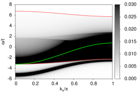
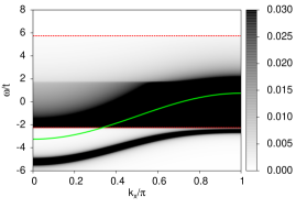
Figure 1: (color online) Energy $E_{\uparrow}(\mathbf{k})$ (thick full green line) and spectral weight $A^{(0)}_{\downarrow}(\mathbf{k},\omega)$ (contour map) vs. $k_{x}$ at $k_{y}=0$, for the Heisenberg model (top) and the Ising model (bottom) in 2D, for AFM coupling $J_{0}/t=3$. The dashed red lines mark the expected continuum boundaries in the $m=1$ subspace. Other parameters are $J/t=0.5,S=0.5,\eta/t=0.01$.

Figure 1 shows $E_{\uparrow}(k_{x},k_{y}=0)$ (thick full green line) and the spectral weight $A^{(0)}_{\downarrow}(k_{x},k_{y}=0,\omega)$ (contour map) for the 2D Heisenberg and Ising models, for antiferromagnetic coupling $J_{0}=3$. The spectrum of the $m=1$ sector consists of a discrete state at low energies, the spin-polaron, and the up-carrier + magnon (c+m) continuum at higher energies. Because we will encounter a different spin-polaron later on, we will refer to this spin polaron as “sp1”. To first order in perturbation theory its effective mass is a factor of $(2S+1)$ larger than the bare carrier mass and its energy is $-J_{0}(S+1)/2+{\cal O}(t,J)$. Berciu and Sawatzky (2009) Most of this energy comes from $\hat{H}^{z}_{\text{exc}}$ and explains why for AFM $J_{0}>0$ sp1 is the ground state – states in the continuum have the carrier with spin up and therefore cost $\sim J_{0}S/2$ in exchange energy. This also suggests that for FM coupling $J_{0}<0$, the sp1 polaron should be located above the c+m continuum. This expectation is confirmed below.

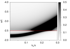
Figure 2: (color online) Top: $A^{(0)}_{\downarrow}(\mathbf{k}=0,\omega)$ for FM $J_{0}/t=-2$ in 2D. The lower c+m continuum edge is marked with dashed red lines. The Ising model has a discrete state (sp2) below the continuum. Bottom: Spectral weight $A^{(0)}_{\downarrow}(\mathbf{k},\omega)$ for the Ising model in 2D for $k_{y}=0,k_{x}<0.3\pi$. The dashed red line marks the lower c+m continuum edge. The sp2 state appears for small $\mathbf{k}$ and then merges into the continuum. Other parameters are $J/t=0.5,S=0.5,\eta/t=0.01$.

Comparing the two panels, we see that the sp1 dispersion is very similar for the two models. This is expected because this is a coherent state where the magnon is locked into a singlet with the carrier, and this process is controlled by $J_{0}\gg J$. A difference appears in the shape of the c+m continuum, however. As mentioned, this must span energies $\{E_{\uparrow}(\mathbf{k}-\mathbf{q})+\Omega_{\mathbf{q}}\}_{\mathbf{q}}$ since it consists of up-carrier and magnon scattering states. The dashed red lines show the boundaries of this range, in agreement with the data (this is more difficult to see for the upper edge, on this scale, due to the reduced spectral weight at high energies). Since Ising magnons are dispersionless the continuum boundaries do not change with $\mathbf{k}$. In contrast, the continuum boundaries for the Heisenberg model vary with $\mathbf{k}$, the continuum being wider at the centre of the Brillouin zone than near its edges.

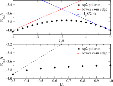
Figure 3: (color online) Ground-state energy of the Ising sp2 polaron as a function of $J_{0}/t$ for $J/t=0.5$ (top) and as a function of $J/t$ for $J_{0}/t=-2$ (bottom), for $S=0.5$.

This difference has consequences for a FM coupling $J_{0}<0$. As mentioned, in this case the c+m continuum is expected to be the low-energy feature in the $m=1$ spectrum, with the sp1 state appearing above it. This is indeed the case for the Heisenberg model, however in the Ising model, for a sufficiently large $J$, a second discrete state emerges below the c+m continuum. We will refer to this state as “sp2” to distinguish it from sp1. The top panel of Fig. 2 shows its presence (absence) for the Ising (Heisenberg) model at $\mathbf{k}=0$. The bottom panel shows that even for the Ising model, the sp2 only exists for small $\mathbf{k}$, at least for these parameters.

The origin of the sp2 state is suggested by the findings of Henning et al. who showed that for $J=0$, polaron-like states exist inside the c+m continuum.Henning et al. (2012) We believe that the addition of $\hat{H}_{\text{I}}$ pushes one of them below the continuum. This is possible because for an Ising coupling, the lower continuum edge moves up by $\Omega=2dJS$, whereas the polaron-like states experience a smaller energy shift since they include a component with the carrier having spin-down. For the Heisenberg model, on the other hand, inclusion of $\hat{H}_{\text{S}}$ does not change the location of the lower continuum edge at $\mathbf{k}=0$ since $\Omega_{\mathbf{q}=0}=0$, so the polaron-like state remains a resonance inside the continuum.

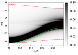
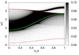
Figure 4: (color online) Spectral weight $A^{(0)}_{\downarrow}(\mathbf{k},\omega)$ vs $k_{x}$ for the 2D Heisenberg model at $k_{y}=0$ (top) and $k_{y}=\pi$ (bottom) and FM $J_{0}/t=-2$. Sp1 appears above the continuum only near the Brillouin zone edge. No sp2 peak is seen below the continuum. The dashed red lines mark the c+m continuum boundaries and the green line marks $E_{\uparrow}(\mathbf{k})$. Other parameters are $J/t=0.5,S=0.5,\eta/t=0.01$.

The ground-state energy of the sp2 polaron is explored in Fig. 3. The top panel shows its dependence on $J_{0}/t$. The sp2 state has weight on both the down-carrier and on the up-carrier+magnon components. For $J_{0}=0$ the weight of the latter component must vanish since no spin-flips are possible and the sp2 state is the same as a free down-carrier, whose energy $-J_{0}S/2-4t$ is also indicated (dashed blue line). These results suggest that as $|J_{0}|/t$ increases, the sp2 state shifts weight from the down-carrier component to the up-carrier+magnon component until it essentially becomes a continuum-like state.

The bottom panel in Fig. 3 shows the sp2 ground-state energy vs. $J/t$ for fixed $J_{0}/t=-2$. This value of $J_{0}/t$ was chosen because here the polaronic character of sp2 is especially strong since if we neglect $H_{\text{exc}}^{x,y}$, the energy of the down-carrier component is equal to that of the up-carrier+magnon component. The distance between sp2 and the continuum increases with $J/t$, as expected from our previous discussion.

While we have only seen the sp2 polaron for the Ising model, we cannot rule out the possibility that for a very narrow range of momenta and carefully chosen parameters, an sp2 state might also appear in the Heisenberg model. Another important point is that the sp1 state is not guaranteed to exist for all $\mathbf{k}$, either. In Fig. 4 we show $A^{(0)}_{\downarrow}(\mathbf{k},\omega)$ for the 2D Heisenberg model. No sp2 state appears below the continuum, and sp1 separates above the continuum only near the Brillouin zone edge. This is not a surprise given the rather small value of $|J_{0}|$, since it controls the separation between sp1 and the continuum. For sufficiently large $|J_{0}|$, the sp1 polaron splits off the continuum in the entire Brillouin zone.Shastry and Mattis (1981)

To summarize, the spectrum in the $m=1$ (one-magnon) subspace contains the expected c+m continuum. For AFM $J_{0}$ the low-energy feature is the sp1 polaron for both the Heisenberg and the Ising models. For FM $J_{0}$, sp1 becomes the high energy feature and may only appear in a small region of the Brillouin zone if $|J_{0}|$ is small. For the Ising model and FM $J_{0}$, an sp2 polaron is also found to appear below the c+m continuum, in a central region of the Brillouin zone that increases with increasing $J$. For the Heisenberg model and FM $J_{0}$ we cannot entirely rule out the existence of sp2, although we provided arguments which suggest that this is unlikely.

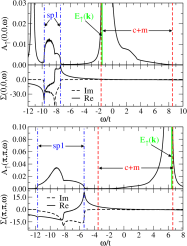
Figure 5: (color online) Spectral weight $A_{\uparrow}(\mathbf{k},\omega)$ and the real (solid line) and imaginary (dashed line) part of the self-energy $\Sigma(\mathbf{k},\omega)$ for the 2D Heisenberg model with AFM $J_{0}/t=10$ and $\beta t=1$, at $\mathbf{k}=(0,0)$ (top) and $\mathbf{k}=(\pi,\pi)$ (bottom). The expected sp1 continuum boundaries are marked with dash-dotted blue lines and the expected c+m continuum boundaries with dashed red lines. The $E_{\uparrow}(\mathbf{k})$ energy of the $T=0$ $\delta$-peak is marked with a thick green line. Other parameters are $J/t=0.5,S=0.5,\eta=0.02$ (top) and $\eta=0.05$ (bottom).

We focused here more on the sp2 polaron because, to our knowledge, this solution had not been discussed before, while the sp1 state has been analyzed in great detail.Shastry and Mattis (1981); Berciu and Sawatzky (2009); Henning et al. (2012); NAKANO et al. (2012) We also note that while we presented only (computationally less costly to generate) 2D results, we find qualitatively similar results in 3D. This will become clear from our finite-T results shown below.

IV.2 Low-T results

We now present and analyze low-T results for the spectral weight of the spin-up carrier. Since the calculation of $G_{\uparrow}(\mathbf{k},\omega)$ becomes numerically very expensive in 3D, most of our analysis is in 2D. However, we will also show a selection of 3D spectra which prove that the 3D results are qualitatively similar to the 2D results.

Figure 6: (color online) Same as Fig. 5 but for the Ising model. All parameters are the same except $\beta t=0.5$ and $\eta=0.01$ in both panels. Note that for the Ising model $\Sigma(\omega)$ is independent of $\mathbf{k}$. The inset shows a zoom on $\Sigma(\omega)$ at high energies.

The spectral weight $A_{\uparrow}(\mathbf{k},\omega)=-\frac{1}{\pi}\text{Im}G_{\uparrow}(\mathbf{k},\omega)$ and the self-energy $\Sigma(\mathbf{k},\omega)$ are shown for the Heisenberg and Ising models with AFM coupling $J_{0}/t=10$ in Figs. 5 and 6, respectively. In both cases the top panel is for $\mathbf{k}=(0,0)$ and the bottom one is for $\mathbf{k}=(\pi,\pi)$. However, for the Ising model the self-energy is independent of $\mathbf{k}$ and therefore in Fig. 6 it is only shown beneath the $k=(0,0)$ spectral weight. The value of $J_{0}/t$ was chosen so large in order to ensure that the different features in the spectrum are well separated, to simplify the analysis. Results for smaller values of $J_{0}$ will be shown below.

$A_{\uparrow}(\mathbf{k},\omega)$, which at $T=0$ is the peak $\delta(\omega-E_{\uparrow}(\mathbf{k}))$ (indicated by the thick green line), broadens into a continuum at finite-$T$. As discussed at the end of Section III, this continuum has its origin in the c+m continuum of the $m=1$ sector, thus we continue to call it the “c+m” continuum, and should span $\{E_{\uparrow}(\mathbf{k+q-q^{\prime}})+\Omega_{\mathbf{q^{\prime}}}-\Omega_{\mathbf{q}}\}_{\mathbf{q,q^{\prime}}}$. The red dashed lines show the boundaries of this energy range, in excellent agreement with the broadening observed in $A_{\uparrow}(\mathbf{k},\omega)$. We note that most of the spectral weight is still located near $E_{\uparrow}(\mathbf{k})$.

This broadening confirms that at finite-T the quasiparticle acquires a finite lifetime (the peak at $E_{\uparrow}(\mathbf{k})$ is now a resonance inside a broad continuum, not a discrete state). Clearly, this is due to processes where the spin-up carrier absorbs a thermal magnon and then re-emits it with a different momentum, thus scattering out of its original state.

The finite lifetime of the carrier in the c+m continuum is also evident in the self-energy. The inset in Fig. 6 shows that for energies within the c+m continuum the imaginary part of the self-energy is finite. The same is true for the Heisenberg model (not shown).

While the broadening of the T=0 $\delta$-peak may be thought of as quite trivial, Figs. 5 and 6 show that it is not the only effect of the finite-T: spectral weight is also transfered to a new continuum located below the c+m continuum. We attribute this continuum to the sp1 state. Indeed, if we denote by $E_{\text{sp1}}(\mathbf{k})$ the energy of the sp1 polaron, we find that this continuum spans $\{E_{\text{sp1}}(\mathbf{k+q})-\Omega_{\mathbf{q}}\}_{\mathbf{q}}$ (the boundaries of this range are marked by the dashed-dotted blue lines). Its presence agrees with the Lehmann representation and reveals this spectral weight transfer to be due to processes where the spin-up carrier binds a thermal magnon and turns into an sp1 polaron.

The sp1 continuum is also where both the real and imaginary part of $\Sigma(\mathbf{k},\omega)$ take their largest values. Consequently the lifetime of these states is roughly two orders of magnitude smaller than that of the states within the c+m continuum. This is not surprising as the c+m continuum stems from a $\delta$-peak with an infinite lifetime at T=0, whereas the sp1 continuum vanishes at T=0.

There is furthermore a qualitative difference between the real-part of $\Sigma(\mathbf{k},\omega)$ in the sp1 continuum and in the c+m continuum. For the latter the real part falls off relatively smoothly (cf. inset in Fig. 6), whereas for the sp1 continuum it is highly singular and almost discontinuous.

Note that there are no major differences between the Heisenberg and Ising models, except for the fact that the boundaries of these continua are momentum dependent for the former and momentum independent for the latter, due to their different magnon dispersions.

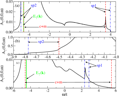
Figure 7: (color online) Spectral weight $A_{\uparrow}(0,0,\omega)$ for the 2D Ising model (panels (a) and (b)) and 2D Heisenberg model (panel (c)) for ferromagnetic $J_{0}/t=-2$ at $\beta t=0.5,\eta/t=0.01$ (Ising) and $\beta t=1,\eta/t=0.02$ (Heisenberg). The expected location of various features are also indicated (see text for more details). Other parameters are $J/t=0.5,S=0.5$.

Figures 5 and 6 also show a very puzzling discrete state at low energies. Before we turn our attention to the analysis of this peak, we quickly discuss the case with FM coupling $J_{0}<0$. Ising and Heisenberg results are depicted in Fig. 7 for $J_{0}/t=-2$ and $J/t=0.5$. From the discussion of the $T=0$ spectrum in the $m=1$ Hilbert space, we know that for these parameters the Ising model has an sp2 state below its c+m continuum and therefore expect to find its signature in the finite-T spectrum, as well. This is indeed the case, as seen more clearly in panel (b) which expands the low-energy part of the Ising spectrum shown in (a), revealing weight at energies spanning $\{E_{\text{sp2}}(\mathbf{k+q})-\Omega_{\mathbf{q}}\}_{\mathbf{q}}$ (its lower boundary is marked by dashed-dotted blue lines). Note that since the sp2 state merges with the c+m continuum (boundaries marked by red dashed lines), their corresponding continua also merge, but panel (b) reveals a clear discontinuity where they overlap. The high-energy sp1 continuum is also clearly observed in panel (a), again merged with the c+m continuum since the sp1 state is not fully separated at such a small $|J_{0}|$, either.

The Heisenberg model (panel (c)) only shows the c+m and sp1 continua, since there is no sp2 polaron here. Again, agreement with the expected boundaries is excellent (the weight seen below the c+m lower edge is due to the finite $\eta$ and the fact that we zoomed in close to the axis to make it easier to see the sp1 continuum).

It is worth noting that since for small $|J_{0}|$ the various features merge, it would be easy to misinterpret the thermal broadening as being all of c+m origin, i.e. to entirely miss the role played by the spin-polaron solutions in the $m=1$ subspace. This is also illustrated in Fig. 8, where we return to an AFM $J_{0}$ coupling and show how the $\mathbf{k}=0$ spectra change as $J_{0}$ is decreased. All features discussed previously can be easily identified for large $J_{0}$ but merge into one another as $J_{0}$ decreases, so that by the time $J_{0}/t=3$ there is only one very broad feature, albeit with a non-trivial structure, left in the spectrum (apart from the low-energy discrete peak, which we will discuss later). If one assumed that this is all of c+m origin, i.e. scattering of the carrier on individual thermal magnons, one would infer very wrong values of the parameters from the boundaries’ locations.

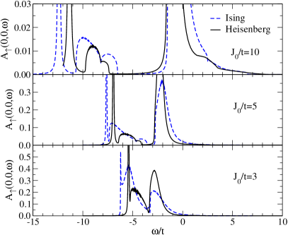
Figure 8: (color online) Spectral weight $A_{\uparrow}(0,0,\omega)$ for the 2D Ising (dashed lines) and Heisenberg (full lines) models for $J_{0}/t=10,5,3$ in the top, middle and bottom panels, respectively. Other parameters are $J/t=0.5,S=0.5$ and $\beta t=0.5,\eta/t=0.01$ (Ising), and $\beta t=1,\eta/t=0.02$ (Heisenberg). The oscillations visible especially in the sp1 continuum are due to finite-size effects (we used $N=100^{2}$ and $N=500^{2}$ for Heisenberg and Ising models, respectively).

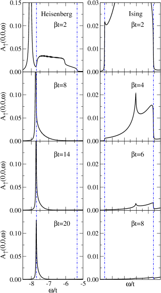
Figure 9: (color online) Spectral weight $A_{\uparrow}(\mathbf{k}=0,\omega)$ for the 2D Heisenberg (left) and Ising (right) models with AFM $J_{0}/t=7$, at different temperatures. Only the sp1 continuum is shown. Its edges are indicated with dot-dashed blue lines Other parameters are $J/t=0.5,S=0.5$ and $\eta/t=0.01$ and $0.02$ for Ising and Heisenberg, respectively.

The results shown so far are for large temperatures $k_{B}T\sim t=2J$ (for our parameters), where higher order corrections should certainly become quantitatively important. On the other hand, from the Lehmann decomposition we expect that the location of the various features does not depend on temperature; only how much spectral weight they carry can change with $T$. For a more thorough analysis we return to the case of AFM $J_{0}$, using a rather large value so that the various features are well separated, and plot in Fig. 9 the spectral weight in the sp1 continuum for several different temperatures, for both the Ising and Heisenberg models. This confirms that, indeed, the weight in this continuum decreases fast as $T\rightarrow 0$ while its location is not affected (the location of the low-energy peak shifts with $T$, but as we argue below, we do not believe that this is a physical feature).

To quantify the spectral weight transferred, we calculate $\int_{\text{c+m}}\mathrm{d}\omega A_{\uparrow}(\mathbf{k},\omega)$, i.e. how much is in the c+m continuum. Since at $T=0$ all the weight is in the $\delta$-peak at $E_{\uparrow}(\mathbf{k})$ located inside the c+m continuum, this value starts at 1 and decreases with increasing $T$, as weight is transferred into the sp1 continuum; one can easily check that the spectral weight obeys the sum rule $\int_{-\infty}^{\infty}\mathrm{d}\omega A_{\uparrow}(\mathbf{k},\omega)=1$.

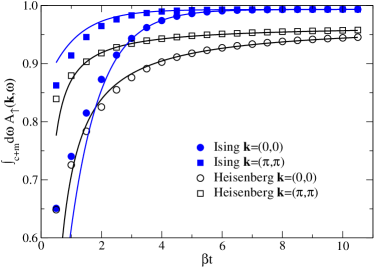
Figure 10: (color online) Integrated spectral weight in the c+m continuum as a function of $\beta$. Lines are fits described in the text. Parameters are: $J_{0}/t=10,J/t=0.5,S=1/2,\eta/t=0.01$ (Ising), $\eta/t=0.05$ (Heisenberg).

The results are shown in Fig. 10 for both models, both at the center and at the corner of the Brillouin zone. Note that because of the finite value of $\eta$, some spectral weight “leaks” outside the continuum’s boundaries. This problem is more severe at lower $T$ because $E_{\uparrow}(\mathbf{k})$ is located very close to an edge of the continuum; this explains why the value saturates below 1 as $\beta\rightarrow\infty$. This explanation is also consistent with the observation that the amount of “missing weight” as $T\rightarrow 0$ is of order $\eta$.

Two features are immediately apparent. First, there is a substantial difference in the amount of spectral weight transferred out of the c+m continuum at $\mathbf{k}=(0,0)$ vs. $\mathbf{k}=(\pi,\pi)$. This is expected for the Heisenberg model where the location of all features changes with $\mathbf{k}$, but may come as a surprise for the Ising model where their location is independent of $\mathbf{k}$. However, for both models $E_{\uparrow}(\mathbf{k})$, where most of the weight is found, moves from the lower edge of the c+m continuum when $\mathbf{k}=0$, to the upper edge for $\mathbf{k}=(\pi,\pi)$. As a result, it is reasonable that weight is transferred into the low-energy sp1 continuum more efficiently at $\mathbf{k}=(0,0)$ than at $\mathbf{k}=(\pi,\pi)$, since in the former case the “effective” energy difference between the two features is smaller.

The second observation is that spectral weight is transferred into the sp1 continuum more efficiently in the Heisenberg model than in the Ising model. This difference is also clearly visible in Fig. 9, where the weight in the sp1 continuum of the Heisenberg model is still respectable at $\beta t=20$, while for the Ising model this weight is already negligible at $\beta t=8$.

An explanation for this difference comes from assuming that the weight in the sp1 continuum is proportional to the average number of thermal magnons, since no sp1 polaron can appear in their absence. Because the Ising magnon spectrum is gapped, at low-$T$ this number is proportional to the Boltzmann factor $\mathrm{e}^{-\beta\Omega}$. This suggests an integrated weight in the c+m spectrum of $a-b\mathrm{e}^{-\beta 4JS}$, where $a=1-\cal{O}(\eta)$ is the limiting value as $T\rightarrow 0$. We fitted the data points for $\beta t>5$ with this form and found a very good fit (solid lines), which moreover works well for a larger range of $\beta$ values than used in the fit.

Magnons of the Heisenberg model are gapless so their number increases much faster with $T$. A simple estimate for a 2D unbounded parabolic dispersion suggests $\langle n\rangle\sim k_{B}T$.note The lines shown for the Heisenberg model in Fig. 10 are fits to $a-b/\beta$ for the data points with $\beta t>5$. The fit is again reasonable over a wider range, and much superior to other simple functional forms we tried, such as $a-b/\beta^{n}$, $n>1$ or $a-b\mathrm{e}^{-\beta cJ}$ (the former assuming that we misindentified the power law, the second to see if Ising-like fits might be more appropriate). Of course, one can find excellent fits for all data using more complicated functions with additional parameters, but they are much harder to justify physically than our simple hypothesis resulting in an effectively one parameter fit.

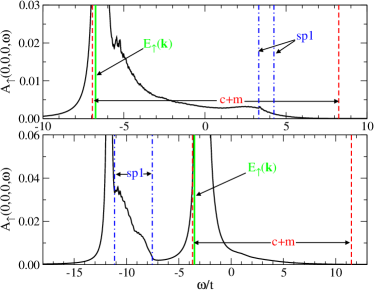
Figure 11: (color online) Spectral weight $A_{\uparrow}(\mathbf{k}=0,\omega)$ for the 3D Heisenberg model at $\beta t=1$ for FM $J_{0}/t=-3$ (top) and AFM $J_{0}/t=10$ (bottom) couplings. The edges of the c+m continuum (dashed red lines) and sp1/sp2 continuum (dot-dashed blue lines) are indicated, as is $E_{\uparrow}(0)$ (thick green line). Other parameters are $J/t=0.5,S=0.5,\eta=0.1$.

Let us now discuss the discrete peak appearing below the sp1 continuum for both models, for AFM $J_{0}$. After carefully investigating many of its properties, such as how its energy and the region in the Brillouin zone where it exists depend on various parameters including $T$,extra we believe that this is an unphysical artefact of our approximation. Arguments for this are: (i) the temperature dependence of its location, clearly visible in Fig. 9 (note that for the Ising model, the peak only separates below the sp1 continuum at higher $T$. At $\beta t=2$ one just starts to see weight piling up near the lower edge, in preparation for this). According to the Lehmann decomposition, the ranges where finite spectral weight is seen cannot vary with $T$; (ii) the fact that the problem is worse at higher-$T$, where we know that higher order corrections ought to be included in the self-energy; these could easily remove an unphysical pole; (iii) the fact that this is a discrete peak, not a resonance inside a continuum (this can be easily verified by checking that its lifetime is set by $\eta$). According to the Lehmann decomposition, discrete peaks cannot appear in the $T\neq 0$ spectral weight. Even if the carrier binds all thermal magnons in a coherent quasiparticle, the finite-$T$ spectral weight would reveal only a continuum associated with it, as is the case for the sp1 and sp2 polarons. To summarize, we believe that this discrete peak is an artefact and that in reality, its weight is part of the sp1 continuum from which it came.

Ideally, these arguments would be strengthened by a calculation of the next correction to the self-energy, to check its effects. We found the exact calculation of the two-magnon term to be daunting even for the Ising model. The difficulty is not so much in evaluating different terms, but in tracing over all possible contributions – so far we did not find a sufficiently efficient way to do this. One can use approximations to speed things up, but that defeats the purpose since it would not be clear if the end results are intrinsic or artefacts, as well. Given this, we cannot entirely rule out that the discrete peak is a (precursor pointing to a) real feature, but we believe that to be very unlikely.

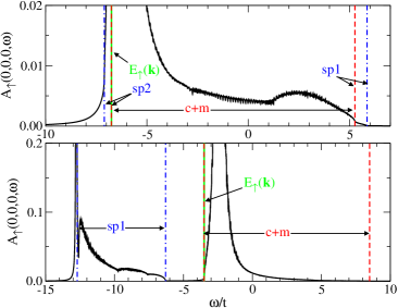
Figure 12: (color online) Spectral weight $A_{\uparrow}(\mathbf{k}=0,\omega)$ for the 3D Ising model at $\beta t=0.5$ for FM $J_{0}/t=-3$ (top) and AFM $J_{0}/t=10$ (bottom) couplings. The edges of the c+m continuum (dashed red lines) and sp1/sp2 continuum (dot-dashed blue lines) are indicated, as is $E_{\uparrow}(0)$ (thick green line). Other parameters are $J/t=0.5,S=0.5,\eta=0.01$.

So far we have done the whole analysis in 2D, simply because the calculation of $\Sigma(\mathbf{k},\omega)$, especially for the Heisenberg model, is numerically much faster. However, we did investigate the 3D models and found essentially the same physics. As examples, in Figs. 11, 12 we show spectra for both FM $J_{0}/t=-3$ and AFM $J_{0}/t=10$, for both models. These spectra display exactly the same features as the corresponding 2D spectra. For the Heisenberg model we chose a larger $\eta=0.1$ and decreased the linear system size drastically to keep the computational time reasonable. Consequently, the continuum edges are more difficult to discern, while finite size effects are more pronounced. In any event, the knowledge accumulated from analysing the 2D data is fully consistent with all features we observed in all 3D data we generated.

V Conclusions

To summarize, we calculated analytically the lowest-$T$ correction to the self-energy of a spin-up carrier injected in a FM background. We used both Heisenberg and Ising couplings to describe the background, to understand the relevance of gapped vs. gapless magnons. These results show how the spectral weight evolves from a discrete peak at $T=0$ to a collection of continua for $T\neq 0$ (these can merge, in the appropriate circumstances), and explain their origin and how their locations can be inferred.

We were aided in this task by the fact that this model conserves the $z$-component of the total spin, allowing us to consider the contribution to the spectral weight coming from Hilbert subspaces with different numbers $m$ of magnons when the carrier has spin up. Although we focused on the $m=1$, lowest-$T$ contribution, based on the knowledge we acquired we can extrapolate with some confidence to higher-$T$, as we discuss now.

One definite conclusion of this work is that knowledge of the $T=0$ carrier spectrum (in the $m=0$ sector) $E_{\uparrow}(\mathbf{k})$, and of the magnon dispersion, $\Omega_{\mathbf{q}}$, is generally not sufficient to predict a priori all features of the finite-$T$ spectral weight, although a fair amount can be inferred from them. To see why, let us assume that magnons do not interact with one another. (This is not true for either model, for example due to their hard-core repulsion; we will return to possible consequences of their interactions below.) If magnons were non-interacting, then Lehmann decomposition of the higher-order contributions in Eq. (7) would predict finite-$T$ spectral weight for all intervals $\{E^{(m)}_{\alpha}(\mathbf{k}+\sum_{i=1}^{m}\mathbf{q}_{i})-\sum_{i=1}^{m}\Omega_{\mathbf{q}_{i}}\}_{\mathbf{q}_{1}+\dots+\mathbf{q}_{m}}$, $m=0,1,\dots$.

Since we move from the $m$ to the $m+1$ subspace by adding a magnon, and given that total momentum is conserved, we know that the spectrum in subspace $m+1$ necessarily includes the convolution between the spectrum of the subspace $m$ and the magnon dispersion, i.e. $\{E^{(m)}_{\alpha}(\mathbf{k}-\mathbf{q})+\Omega_{\mathbf{q}}\}_{\mathbf{q}}$ is part of the spectrum $E^{(m+1)}_{\alpha}(\mathbf{k})$ (these are the scattering states between the extra magnon and any eigenstate in the $m$ spectrum).

This observation allows us to infer the location of some of the finite-$T$ spectral weight, by recurrence. $E^{(1)}_{\alpha}(\mathbf{k})$ must include all scattering states $\{E_{\uparrow}(\mathbf{k}-\mathbf{q})+\Omega_{\mathbf{q}}\}_{\mathbf{q}}$, so the $m=1$ contribution to the spectrum must span $\{E^{(1)}_{\alpha}(\mathbf{k}+\mathbf{q}^{\prime})-\Omega_{\mathbf{q}^{\prime}}\}_{\mathbf{q}^{\prime}}=\{E_{\uparrow}(\mathbf{k}-\mathbf{q}+\mathbf{q}^{\prime})-\Omega_{\mathbf{q}^{\prime}}+\Omega_{\mathbf{q}}\}_{{\mathbf{q}},{\mathbf{q}^{\prime}}}$. We called this the c+m continuum and verified that it is indeed seen in the finite-$T$ spectral weight. Knowledge of this part of the $m=1$ spectrum allows us to infer scattering states that are part of the $m=2$ spectrum and therefore their Lehmann contribution, etc. The conclusion is that all intervals $\{E_{\uparrow}(\mathbf{k}+\sum_{i=1}^{m}\mathbf{q}^{\prime}_{i}-\sum_{i=1}^{m}\mathbf{q}_{i})-\sum_{i=1}^{m}\Omega_{\mathbf{q}^{\prime}_{i}}+\sum_{i=1}^{m}\Omega_{\mathbf{q}_{i}}\}_{{\mathbf{q}_{1}},\dots,{\mathbf{q}^{\prime}_{m}}}$ will contain some spectral weight at finite-$T$. For the dispersionless Ising magnons this interval is the same for all $m$. For dispersive Heisenberg magnons this interval broadens with $m$. For very small $J$, the additional broadening as $m$ increases is very small and moreover one would expect little spectral weight in the high-$m$ sectors if the $T$ is not too large. Thus, we expect weight to be visible in the c+m continuum up to high(er) temperatures; its boundaries may also slowly expand with $T$, for a Heisenberg background, as higher $m$ subspaces become thermally activated.

Apart from these scattering states, $E^{(m+1)}_{\alpha}(\mathbf{k})$ might also contain bound states where the extra magnon is coherently bound to all the other particles. The existence and location of such coherent states cannot be predicted a priori, as they depend on the details of the model (however, they certainly cannot appear unless coherent states exist in the $m$ space). An example is the $E^{(1)}_{\alpha}(\mathbf{k})$ spectrum which indeed contains the scattering states discussed above, but also contains the sp1 and/or sp2 discrete polarons states. These give rise to their own continua of scattering states in higher $m$ subspaces, whose locations can be inferred by recurrence.

The question, then, is if it is likely to find such new, bound coherent states for all values of $m$, i.e. if the number of additional continua becomes arbitrarily large with increasing $T$. Generally, the answer must be “no”, since this requires bound states between arbitrarily large numbers of objects. For the problem at hand, we believe that it is quite unlikely that they appear even in the $m=2$ subspace, since that would involve one carrier binding two magnons. This is a difficult task given the weak nearest-neighbour attraction of order $J$ between magnons (due to the breaking of fewer FM bonds), and the fact that the carrier can interact with only one magnon at a time. The exception is likely to be in 1D systems where magnons can coalesce into magnetic domains.

Let us now consider the role of magnon interactions. Because of them, many-magnon states are not eigenstates of the Heisenberg Hamiltonian so higher-order terms are not obtained by tracing over states with many independent magnons (in the Ising model this complication can be avoided by working in real space). If the attraction between magnons is too weak to bind them, this is not an issue since their spectra will still consist of scattering states spanning the same energies like for non-interacting magnons. As a result, the location of various features is not affected, but the distribution of the spectral weight inside them will be since the eigenfunctions are different. Magnon pairing is unlikely for $d>1$ unless the exchange is strongly anisotropic. However, if it happens and if the spectrum of the magnon pairs is known, one could infer its effects on the carrier spectral weight just like above.

Based on these arguments, we expect the higher-$T$ spectral weight to show the same features we uncovered at low-$T$ (the distribution of the weight between them might be quite different, though). These expectations could be verified with numerical simulations (conversely, our low-$T$ results can be used to test codes). Such simulations would also solve the issue of the discrete peak that we observed for AFM $J_{0}$, and which we argued to be an artefact of our low-$T$ approximation.

To conclude, although quantitatively our results are only valid at extremely low-$T$, we believe that this study clarifies qualitatively how the spectral weight of a spin-up carrier evolves with $T$. Our arguments can be straightforwardly extended to predict what features appear in the spectral weight of a spin-down carrier, as well.

A general feature demonstrated by our work is that finite-$T$ does not result in just a simple thermal broadening of the quasiparticle peak, as it becomes a resonance inside a continuum. Spectral weight can also be transferred to quite different energies if the quasiparticle can bind additional magnons into coherent polarons. When this happens, interpretation of experimentally measured and/or of computationally generated spectra could become difficult, unless one is aware of this possibility.

Appendix A Derivation of the lowest $T\neq 0$ self-energy term

We present this calculation for the Heisenberg FM; the Ising case is treated similarly. To find $G_{\uparrow}^{(1)}(\mathbf{k},\mathbf{q},\mathbf{q}^{\prime},\omega)$, we divide $\hat{H}=\hat{H}_{0}+\hat{V}$ where $\hat{H}_{0}=\hat{T}+\hat{H}_{\text{S}}^{z}$ and $\hat{V}=\hat{H}_{\text{S}}^{x,y}+\hat{H}_{\text{exc}}$, and use Dyson’s identity $\hat{G}(\omega)=\hat{G}_{0}(\omega)+\hat{G}(\omega)\hat{V}\hat{G}_{0}(\omega)$ where $\hat{G}_{0}=[\omega-\hat{H}_{0}+i\eta]^{-1}$ is the resolvent for $\hat{H}_{0}$. This procedure is similar to that used in Ref. Berciu and Sawatzky, 2009 for the $T=0$ spin-polaron. Applying Dyson’s identity once we obtain:

$$G_{\uparrow}^{(1)}(\mathbf{k},\mathbf{q},\mathbf{q}^{\prime},\omega)=G^{(0)}_{\uparrow}(\mathbf{k+q^{\prime}-q},\omega+\Omega_{\mathbf{q^{\prime}}}-\Omega_{\mathbf{q}})\left[\delta_{\mathbf{q},\mathbf{q^{\prime}}}\right.$$

$$\left.-\frac{J_{0}}{2N}\sum_{\mathbf{Q}}G_{\uparrow}^{(1)}(\mathbf{k},\mathbf{Q},\mathbf{q}^{\prime},\omega)+J_{0}\sqrt{\frac{S}{2N}}F(\mathbf{k},\mathbf{q},\omega)\right]$$ (13)

The first term on the right-hand side is just the diagonal term. The second term accounts for the energy shift that occurs when the up-carrier is on the same site as the magnon, and the third term contains a new propagator $F(\mathbf{k},\mathbf{q^{\prime}},\omega)=\langle\Phi(\mathbf{q^{\prime}})|c_{\mathbf{k},\uparrow}\hat{G}(\omega+\Omega_{q^{\prime}})c_{\mathbf{k+q},\downarrow}^{\dagger}|{\rm FM}\rangle$. This term accounts for spin-flip processes where the up-carrier absorbs the magnon, turning into a down-carrier with momentum $\mathbf{k+q}$. Using Dyson’s identity again, we get an equation of motion for $F(\mathbf{k},\mathbf{q^{\prime}},\omega)$:

$$F(\mathbf{k},\mathbf{q^{\prime}},\omega)= J_{0}\sqrt{\frac{S}{2N}}G^{(0)}_{\uparrow}(\mathbf{k+q},\omega+\Omega_{\mathbf{q^{\prime}}}+J_{0}S)$$

$$\times\sum_{\mathbf{Q}}G_{\uparrow}^{(1)}(\mathbf{k},\mathbf{Q},\mathbf{q}^{\prime},\omega).$$ (14)

The diagonal element vanishes since the bra and ket are orthogonal. The energy shift $-J_{0}S/2$ of the spin-down carrier is absorbed into the argument of $G^{(0)}_{\uparrow}$, leaving only the spin-flip process which links $F$ back to $G_{\uparrow}^{(1)}$.

These two coupled equations can now be solved as follows. We insert Eq. (14) into Eq. (13) to obtain:

$$G_{\uparrow}^{(1)}(\mathbf{k},\mathbf{q},\mathbf{q}^{\prime},\omega)=G^{(0)}_{\uparrow}(\mathbf{k+q^{\prime}-q},\omega+\Omega_{\mathbf{q^{\prime}}}-\Omega_{\mathbf{q}})\left\{\delta_{\mathbf{q},\mathbf{q^{\prime}}}\right.$$

$$\left.-\frac{J_{0}}{2}f(\mathbf{k},\mathbf{q^{\prime}},\omega)\left[1-J_{0}SG^{(0)}_{\uparrow}(\mathbf{k+q},\omega+\Omega_{\mathbf{q^{\prime}}}+J_{0}S)\right]\right\},$$ (15)

where $f(\mathbf{k},\mathbf{q^{\prime}},\omega)=\frac{1}{N}\sum_{\mathbf{Q}}G_{\uparrow}^{(1)}(\mathbf{k},\mathbf{Q},\mathbf{q^{\prime}},\omega)$. Using Eq. (15) in the definition of $f(\mathbf{k},\mathbf{q^{\prime}},\omega)$ yields:

$$f(\mathbf{k},\mathbf{q^{\prime}},\omega)=\frac{1}{N}G^{(0)}_{\uparrow}(\mathbf{k},\omega)\left[1+\frac{J_{0}}{2}g(\mathbf{k},\mathbf{q^{\prime}},\omega)\right.$$

$$\left.\times\left(1-J_{0}SG^{(0)}_{\uparrow}(\mathbf{k+q^{\prime}},\omega+J_{0}S)\right)\right]^{-1},$$

with $g(\mathbf{k},\mathbf{q^{\prime}},\omega)=\frac{1}{N}\sum_{\mathbf{Q}}G^{(0)}_{\uparrow}(\mathbf{k+q^{\prime}-Q},\omega+\Omega_{\mathbf{q^{\prime}}}-\Omega_{\mathbf{Q}}).$ Note that $g(\mathbf{k},\mathbf{q^{\prime}},\omega)$ can be calculated numerically since $G^{(0)}_{\uparrow}(\mathbf{k},\omega)$ is a known function.

All that is left to do is to insert the above expression into Eq. (15) and calculate $\sum_{\mathbf{q}}\mathrm{e}^{-\beta\Omega_{\mathbf{q}}}G_{\uparrow}^{(1)}(\mathbf{k},\mathbf{q},\mathbf{q},\omega)$, to find the expression listed in Section III.

References

- (1) J. Z. Bednorz and K. A. Müller, Z. Phys. B 64, 189 (1986); P. A. Lee, N. Nagaosa, and X-G Wen, Rev. Mod. Phys. 78, 17 (2006).
- Ramirez (1997) A. P. Ramirez, J. Phys: Cond. Matt. 9, 8171 (1997).
- Nolting et al. (2001) W. Nolting, G. G. Reddy, A. Ramakanth, and D. Meyer, Phys. Rev. B 64, 155109 (2001).
- (4) X. Liu, T. Berlijn, W.-G. Yin, W. Ku, A. Tsvelik, Y.-J. Kim, H. Gretarsson, Y. Singh, P. Gegenwart, and J. P. Hill, Phys. Rev. B 83, 220403 (2011); Y. Singh, S. Manni, J. Reuther, T. Berlijn, R. Thomale, W. Ku, S. Trebst, and P. Gegenwart, Phys. Rev. Lett. 108, 127203 (2012).
- (5) H. Ohno, A. Shen, F. Matsukura, A. Oiwa, A. Endo, S. Katsumoto and Y. Iye, Appl. Phys. Lett. 69, 363 (1996); T. Dietl, Nature Materials 2, 646 (2003).
- Lee et al. (1987) W. H. Lee, R. N. Shelton, S. K. Dhar, and K. A. Gschneidner, Phys. Rev. B 35, 8523 (1987).
- Wolf et al. (2001) S. A. Wolf, D. D. Awschalom, R. A. Buhrman, J. M. Daughton, S. v. Molnár, M. L. Roukes, A. Y. Chtchelkanova, and D. M. Treger, Science 294, 1488 (2001), PMID: 11711666.
- (8) B. Lau, M. Berciu and G. A. Sawatzky, Phys. Rev. Lett. 106, 036401 (2011).
- Shastry and Mattis (1981) B. S. Shastry and D. C. Mattis, Phys. Rev. B 24, 5340 (1981).
- Berciu and Sawatzky (2009) M. Berciu and G. A. Sawatzky, Phys. Rev. B 79, 195116 (2009).
- Henning et al. (2012) S. Henning, P. Herrmann, and W. Nolting, Phys. Rev. B 86, 085101 (2012).
- NAKANO et al. (2012) K. Nakano, R. Eder, and Y. Ohta, Int. J. Mod. Phys. B 26, 1250154 (2012).
- (13) M. Möller, G. A. Sawatzky and M. Berciu, Phys. Rev. Lett. 108, 216403 (2012); ibid, Phys. Rev. B 86, 075128 (2012).
- Nolting et al. (1997) W. Nolting, S. Rex, and S. M. Jaya, J. Phys: Cond. Matt. 9, 1301 (1997).
- Nolting and Matlak (1984) W. Nolting and M. Matlak, physica status solidi (b) 123, 155–168 (1984).
- (16) D. N. Zubarev, Sov. Phys. Usp. 3, 320 (1960).
- (17) The prefactor contains the Riemann number . However, this approximation ignores non-parabolic corrections to the dispersion and lacks the equivalent of a “Debye energy”, instead summing over all energies. Including such corrections should remove the singularity.
- (18) M. Möller (unpublished).