Optical potential from first principles

Abstract

We develop a method to construct a microscopic optical potential from chiral interactions for nucleon-nucleus scattering. The optical potential is constructed by combining the Green’s function approach with the coupled-cluster method. To deal with the poles of the Green’s function along the real energy axis we employ a Berggren basis in the complex energy plane combined with the Lanczos method. Using this approach, we perform a proof-of-principle calculation of the optical potential for the elastic neutron scattering on ${}^{16}{\rm O}$. For the computation of the ground-state of ${}^{16}{\rm O}$, we use the coupled-cluster method in the singles-and-doubles approximation, while for the $A=\pm 1$ nuclei we use particle-attached/removed equation-of-motion method truncated at two-particle-one-hole and one-particle-two-hole excitations, respectively. We verify the convergence of the optical potential and scattering phase shifts with respect to the model-space size and the number of discretized complex continuum states. We also investigate the absorptive component of the optical potential (which reflects the opening of inelastic channels) by computing its imaginary volume integral and find an almost negligible absorptive component at low-energies. To shed light on this result, we computed excited states of ${}^{16}{\rm O}$ using equation-of-motion coupled-cluster method with singles-and-doubles excitations and we found no low-lying excited states below 10 MeV. Furthermore, most excited states have a dominant two-particle-two-hole component, making higher-order particle-hole excitations necessary to achieve a precise description of these core-excited states. We conclude that the reduced absorption at low-energies can be attributed to the lack of correlations coming from the low-order cluster truncation in the employed coupled-cluster method.

I Introduction

Nuclear reactions are the ubiquitous experimental tool to study atomic nuclei. While many astrophysically relevant reactions proceed at relatively low energies $E<1$ MeV Thompson and Nunes (2009), in the laboratory, these reactions are often studied indirectly with beams at higher energy ($\geq$5 MeV/u). One of the most important open questions currently being explored today in our field concerns the astrophysical site for the r-process, the process that gave rise to about half of the heavy elements in our planet. In order to perform simulations of neutron star mergers or supernovae explosions (the two possible sites under consideration), neutron capture rates are needed on rare isotopes of nuclei as heavy as Uranium Thompson and Nunes (2009). Despite all the effort with ab initio approaches to nuclear reactions, which include the study of elastic scattering Nollett et al. (2007); Quaglioni and Navrátil (2008); Hagen and Michel (2012); Hupin et al. (2013); Elhatisari et al. (2015); Mazur et al. (2015), transfer Navrátil and Quaglioni (2012), photo reactions Gazit et al. (2006); Efros et al. (2007); Bacca et al. (2014), and capture reactions Girlanda et al. (2010); Marcucci et al. (2013), only selected nuclei and specific reaction channels can be addressed with the various ab-initio methods in the market (Refs. Bacca and Pastore (2014); Navrátil et al. (2016) for recent reviews).

A more general approach to reactions involving heavier nuclei is based on a reduction of the many-body picture to a few-body one, where only the most relevant degrees of freedom are retained Thompson and Nunes (2009). In such approaches one introduces effective interactions (the so-called optical potentials) between the clusters considered. Traditionally these interactions have been constrained by data, particularly using data on $\beta$-stable isotopes Koning and Delaroche (2007); Capote et al. (2009). Clearly, the application of these global parameterizations to exotic regions of the nuclear chart is unreliable and has uncontrolled uncertainties. It is critical for progress in the field of reactions that these effective interactions be connected to the underlying microscopic theory so that extrapolations to exotic regions can be better understood.

In most cases, phenomenological optical potentials are made local for simplicity. We know based on the Feshbach projection formalism that, in its most general form, the microscopic optical potential should be complex, non-local and energy dependent H.Feshbach (1958, 1962). Recently, a series of studies has shown that nonlocality can affect transfer reaction observables (e.g. Titus and Nunes (2014); Ross et al. (2015); Titus et al. (2016)) and it is expected that it can equally affect other reaction channels. So far we have not been able to identify an experimental method to constrain nonlocality. It is essential that microscopic theories provide guidance on this aspect of the optical potential.

The goal of this work is to provide a proof-of-principle for a new method to compute nuclear optical potentials from ab-initio many-body coupled cluster calculations. It is the first of a series of studies that aims at constructing an optical potential rooted in the underlying microscopic formulation of the problem, potentials which can then be incorporated, consistently with other ingredients, into the general few-body formalism. In an approach based on Feshbach projection operators, the optical potential is the self-energy term in the Dyson equation F.Capuzzi and C.Mahaux (1996). Semiphenomenological optical potential have been obtained using approximation of the self-energy at the Brueckner-Hartree-Fock level Jeukenne et al. (1976). For the scattering of nucleons at high energy ($\geq$ 100 MeV) optical potential can be derived with the multiple scattering formalism Kerman et al. (1959). More recently, the solution of the Dyson equation by self-consistent Green’s function methods has been used to compute optical potentials Dickhoff and Barbieri (2004); Barbieri and Jennings (2005); Mahzoon et al. (2014). In this paper, we compute the Green’s function directly following the coupled cluster method Kümmel et al. (1978); Hagen et al. (2014), thus circumventing the usual self-consistency approach. The self-energy can then be determined by inverting the Dyson equation. The key elements in our approach to compute the Green’s function are: i) an analytical continuation in the complex energy plane based on a Berggren basis consisting of bound, resonant, and non-resonant scattering states Berggren (1968); Michel et al. (2002); Id Betan et al. (2002); Hagen et al. (2004); Hagen and Vaagen (2006), and ii) a generalized non-symmetric Lanczos method Cullum (1998) that allows us to write the Green’s function as a continued fraction Dagotto (1994); Hallberg (1995); Efros et al. (2007); Bacca et al. (2014). The first of these two elements is essential because it allow us to properly deal with the poles of the Green’s function along the real energy axis, and obtain numerically stable Green’s functions and optical potentials. The second element is essential to make the problem computationally feasible. In this work we demonstrate that optical potentials, converged with respect to the models space, can indeed be determined from the Green’s functions generated from coupled cluster many-body calculations. We note that the computation of Green’s functions with the coupled-cluster method is well established in quantum chemistry Nooijen and Snijders (1992, 1993, 1995), and that very recently this approach has also been used to extract the optical potential Bhaskaran-Nair et al. (2016). Our approach is similar to that effort, but applied to nuclear many-body problem.

This paper is organized as follows. In Sec. (II) we introduce the formalism of the Green’s function and the coupled-cluster method along with the Berggren basis and discuss the application of the Lanczos method for the numerical calculations of the Green’s function. In Sec. III, we show an application for the elastic scattering on ${\rm{}^{16}O}$ and discuss the results. Finally, we will conclude and discuss future possible applications in Sec. IV.

II Formalism

II.1 The single-particle Green’s function

The single-particle Green’s function of an $A$-nucleon system has matrix elements

$$G(\alpha,\beta,E) = \langle\Psi_{0}|a_{\alpha}\frac{1}{E-(H-E^{A}_{gs})+i\eta}a^{\dagger}_{\beta}|\Psi_{0}\rangle$$ (1)

$$+ \langle\Psi_{0}|a^{\dagger}_{\beta}\frac{1}{E-(E^{A}_{gs}-H)-i\eta}a_{\alpha}|\Psi_{0}\rangle.$$

Here, $\alpha$ and $\beta$ denote single-particle states, and $|\Psi_{0}\rangle$ is the ground state of the $A$-body system with energy $E^{A}_{gs}$. As usual, the parameter $\eta\geq 0$ is such that $\eta\rightarrow 0$ at the end of the calculation. The operators $a^{\dagger}_{\alpha}$ and $a_{\beta}$ create and annihilate a fermion in the single-particle state $\alpha$ and $\beta$, respectively, and are shorthands for the quantum numbers $\alpha=(n,l,j,j_{z},\tau_{z})$. Here, $n,l,j,j_{z},\tau_{z}$ label the radial quantum number, the orbital angular momentum, the total orbital momentum, its projection on the $z-$ axis, and the isospin projection, respectively. The intrinsic Hamiltonian $H$ is

$$H=\sum^{A}_{i=1}\frac{\vec{p_{i}}^{2}}{2m}-\frac{\vec{P}^{2}}{2mA}+\sum_{i<j}V_{ij}.$$ (2)

Here, $\vec{p}_{i}$ is the momentum of the nucleon $i$ of mass $m$ and $\vec{P}=\sum_{i=1}^{A}\vec{p}_{i}$ is the momentum associated with the center of mass motion. We limit ourselves to a two-body interactions $V_{ij}$ and neglect contributions from three-nucleon forces. It is useful to rewrite the Hamiltonian as

$$H=\sum^{A}_{i=1}\frac{\vec{p}_{i}^{2}}{2m}\left(1-\frac{1}{A}\right)+\sum_{i<j}\left(V_{ij}-\frac{\vec{p}_{i}\vec{p}_{j}}{mA}\right),$$ (3)

separating one-body and two-body contributions. In what follows, we take the single-particle states from the Hartree-Fock (HF) basis. We recall that the HF basis is an excellent starting point for coupled-cluster calculations and that the HF Green’s function

$$G^{(0)}(\alpha,\beta,E) = \langle\Phi_{0}|a_{\alpha}\frac{1}{E-(H_{0}-E^{A}_{gs,0})+i\eta}a^{\dagger}_{\beta}|\Phi_{0}\rangle$$ (4)

$$+ \langle\Phi_{0}|a^{\dagger}_{\beta}\frac{1}{E-(E^{A}_{gs,0}-H_{0})-i\eta}a_{\alpha}|\Phi_{0}\rangle$$

is a first order approximation to the Green’s function (1). In Eq. (4) $H_{0}$ is the HF potential, $|\Phi_{0}\rangle$ the HF reference state of the $A$-nucleon system and $E^{A}_{gs,0}$ the corresponding energy. As the single-particle states $\alpha,\beta$ are given by the HF basis, Eq. (4) can be written as

$$G^{(0)}(\alpha,\beta,E)=\delta_{\alpha,\beta}\left[\frac{\Theta(\alpha-F)}{E-\varepsilon_{\alpha}+i\eta}+\frac{\Theta(F-\alpha)}{E-\varepsilon_{\alpha}-i\eta}\right].$$ (5)

Here, $\varepsilon_{\alpha}$ is the single-particle energy associated with $|\alpha\rangle$ and $\Theta$ the unit step function. For a single-particle state $\alpha$ above the occupied shells in the HF approximation, $\Theta(\alpha-F)=1$, whereas $\Theta(\alpha^{\prime}-F)=0$ for $\alpha^{\prime}$ below the Fermi level.

The Green’s function fulfills the Dyson equation

$$G(\alpha,\beta,E) = G^{(0)}(\alpha,\beta,E)$$ (6)

$$+ \sum_{\gamma,\delta}G^{(0)}(\alpha,\gamma,E)\Sigma^{*}(\gamma,\delta,E)G(\delta,\beta,E).$$

Here, $\Sigma^{*}(\gamma,\delta,E)$ is the self energy, which can be obtained from the inversion of Eq. (6):

$$\Sigma^{*}(E)=[G^{(0)}(E)]^{-1}-G^{-1}(E).$$ (7)

To obtain the optical potential we introduce the quantity

$$\Sigma^{\prime}\equiv\Sigma^{*}+U,$$ (8)

where $U$ is the HF potential. For $E\geq E^{A}_{gs}$, $\Sigma^{\prime}$ in Eq. (8) corresponds to the optical potential for the elastic scattering from the $A$-nucleon ground state F.Capuzzi and C.Mahaux (1996); Dickhoff and Neck (2007). We are interested in the scattering amplitude

$$\xi_{E^{+}}({\bf r})=\langle\Psi_{0}|a_{{\bf r}}|\Psi_{E+}\rangle$$ (9)

where $|\Psi_{E^{+}}\rangle$ is the elastic scattering state of a nucleon on the target with the energy $E^{+}=E-E^{A}_{gs}$ and $a_{\bf{r}}$ the annihilation operator of a particle at the position ${\bf{r}}$. The scattering amplitude $\xi^{c}_{E^{+}}(r)$ is the solution of the Schrödinger equation containing the optical potential

$$-\frac{\hbar^{2}}{2\mu}\nabla^{2}\xi({\bf r})+\int d{\bf r^{\prime}}\Sigma^{\prime}({\bf r},{\bf r^{\prime}},E^{+})\xi({\bf r^{\prime}})=E^{+}\xi({\bf r}).$$ (10)

where $\mu$ is the reduced mass of the nucleus-nucleon system. For simplicity, we suppressed any spin and isospin labels. The optical potential is non-local, energy-dependent and complex Dickhoff and Neck (2007) and, for $E^{+}\geq 0$, its imaginary component describes the loss of flux due to absorption. Similarly, the overlap $\xi_{n}({\bf r})=\langle\Psi_{0}|a_{\bf{r}}|\Psi^{A+1}_{n}\rangle$ for a bound state $|\Psi^{A+1}_{n}\rangle$ of energy $E_{n}^{A+1}$ in the $A+1$ system, fulfills the Schrödinger equation with the optical potential at the discrete energy $E_{n}=E_{n}^{A+1}-E^{A}_{gs}$.

In this paper, we construct the optical potential by an inversion of the Dyson equation (6) after a direct computation of the Green’s function (1) following the coupled-cluster method Hagen et al. (2014). In the following section, we present the main steps involved in the computation of the Green’s function in our approach.

II.2 Green’s function from coupled-cluster method

The HF reference state for the nucleus consisting of $A$ nucleons is

$$|\Phi_{0}\rangle=\Pi_{i=1}^{A}a^{\dagger}_{i}|0\rangle.$$ (11)

In coupled-cluster theory, see Refs. Bartlett and Musiał (2007); Hagen et al. (2014) for details, the ground state is represented as

$$|\Psi_{0}\rangle=e^{T}|\Phi_{0}\rangle,$$ (12)

and $T$ denotes the cluster operator

$$T = T_{1}+T_{2}+\dots$$ (13)

$$= \sum_{i,a}t_{i}^{a}a^{\dagger}_{a}a_{i}+\frac{1}{4}\sum_{ijab}t_{ij}^{ab}t_{ijab}a^{\dagger}_{a}a^{\dagger}_{b}a_{j}a_{i}+\ldots.$$

We note that $T_{1}$ and $T_{2}$ induce $1p$-$1h$ and $2p$-$2h$ excitations of the HF reference, respectively. Here and in what follows, the single-particle states $i,j,...$ refer to hole states occupied in the reference state $|\Phi_{0}\rangle$ while $a,b,...$ denote valence states above the reference state. In practice, the expansion (13) is truncated. In the coupled cluster with singles and doubles (CCSD) all operators $T_{i}$ with $i>2$ are neglected. In that case, the ground-state energy and the amplitudes $t_{i}^{a},t_{ij}^{ab}$ are obtained by projecting the state (12) on the reference state and on all $1p$-$1h$ and $2p$-$2h$ configurations for which

$$\langle\Phi_{0}|\overline{H}|\Phi_{0}\rangle = E,$$

$$\langle\Phi_{i}^{a}|\overline{H}|\Phi_{0}\rangle = 0,$$

$$\langle\Phi_{ij}^{ab}|\overline{H}|\Phi_{0}\rangle = 0.$$ (14)

Here,

$$\overline{H} \equiv e^{-T}He^{T}$$ (15)

$$= H+\left[H,T\right]+{1\over 2!}\left[\left[H,T\right],T\right]+\ldots$$

denotes the similarity transformed Hamiltonian and it can be computed systematically via the Baker-Campbell-Hausdorff expansion. For two-body forces and in the CCSD approximation, this expansion actually terminates at fourfold nested commutators.

The CCSD equations (II.2) show that the CCSD ground state is an eigenstate of the similarity-transformed Hamiltonian in the space of $0p$-$0h$, $1p$-$1h$, $2p$-$2h$ configurations. The transformed Hamiltonian is not Hermitian because the operator $e^{T}$ is not unitary. As a consequence, $\overline{H}$ has left- and right-eigenvectors which constitute a bi-orthogonal basis with the corresponding completeness relation

$$\sum_{i}|\Phi_{i,R}\rangle\langle\Phi_{i,L}|=\hat{{1}}.$$ (16)

The right ground state is the reference state $|\Phi_{0}\rangle$, while the left ground-state is given by $\langle\Phi_{0,L}|=\langle\Phi_{0}|(1+\Lambda)$ where $\Lambda$ is a linear combination of particle-hole de-excitation operators.

Using the ground state of the similarity-transformed Hamiltonian, we now can write the coupled cluster Green’s function $G^{CC}$ as

$$G^{CC}(\alpha,\beta,E)\equiv$$ (17)

$$\langle\Phi_{0,L}|\overline{a_{\alpha}}\frac{1}{E-(\overline{H}-E^{A}_{gs})+i\eta}\overline{a^{\dagger}_{\beta}}|\Phi_{0}\rangle$$

$$+ \langle\Phi_{0,L}|\overline{a^{\dagger}_{\beta}}\frac{1}{E-(E^{A}_{gs}-\overline{H})-i\eta}\overline{a_{\alpha}}|\Phi_{0}\rangle.$$

Here, $\overline{a_{\alpha}}=e^{-T}a_{\alpha}e^{T}$ and $\overline{a^{\dagger}_{\beta}}=e^{-T}a^{\dagger}_{\beta}e^{T}$ are the similarity-transformed annihilation and creation operators, respectively, and the Baker-Campbell-Hausdorff expansion yields the relations

$$\overline{a_{\alpha}} = a_{\alpha}+[a_{\alpha},T],$$ (18)

$$\overline{a^{\dagger}_{\beta}} = a^{\dagger}_{\beta}+[a^{\dagger}_{\beta},T].$$ (19)

We note that the truncation of the cluster operator $T$ is reflected in the expression of the coupled-cluster Green’s function (17), and if all excitations up to $Ap$-$Ah$ were taken into account in the expansion (13), the Green’s function (17) would be identical to (1).

One might be tempted to use the completeness relations for the $A\pm 1$ systems to obtain the Lehmann representation of the Green’s function

$$G^{CC}(\alpha,\beta,E)=$$ (20)

$$\sum_{i}\frac{\langle\Phi_{0,L}|\overline{a_{\alpha}}|\Phi^{A+1}_{i}\rangle\langle\Phi^{A+1}_{i}|\overline{a^{\dagger}_{\beta}}|\Phi_{0}\rangle}{E-(E^{A+1}_{i}-E^{A}_{gs})+i\eta}$$

$$+ \sum_{j}\frac{\langle\Phi_{0,L}|\overline{a^{\dagger}_{\beta}}|\Phi^{A-1}_{j}\rangle\langle\Phi^{A-1}_{j}|\overline{a_{\alpha}}|\Phi_{0}\rangle}{E-(E^{A}_{gs}-E^{A-1}_{j})-i\eta}.$$

Here, $|\Phi^{A+1}_{i}\rangle$ ($|\Phi^{A-1}_{j}\rangle$) is an eigenstate of $\overline{H}$ for the $A+1$ ($A-1$) system with energy $E^{A+1}_{i}$ ($E^{A-1}_{j}$). To simplify the notation, the completeness relations are written in (20) as discrete summations over the states in the $A\pm 1$ systems. In principle, the Green’s function (20) could be obtained by calculating the spectrum of the $A\pm 1$ systems using the particle-attached equation-of-motion (PA-EOM) and particle-removed equation-of-motion (PR-EOM) coupled-cluster methods Gour et al. (2006). However in practice, this approach is difficult to pursue as the sum over all states also involves eigenstates in the continuum. To avoid this problem, we return to the expression in Eq. (17) and use the Lanczos technique Efros et al. (2007); Bacca et al. (2014) for its computation.

II.3 Lanczos method

In this section, we describe the calculation of the coupled-cluster Green’s function (17) using the Lanczos method Dagotto (1994); Hallberg (1995); Efros et al. (2007); Bacca et al. (2014). To simplify the notation we introduce the following shorthands

$$|v^{A+1}_{\beta}\rangle \equiv \overline{a^{\dagger}_{\beta}}|\Phi_{0}\rangle,$$ (21)

$$\langle u^{A+1}_{\alpha}| \equiv \langle\Phi_{0,L}|\overline{a_{\alpha}},$$ (22)

$$|v^{A-1}_{\alpha}\rangle \equiv \overline{a_{\alpha}}|\Phi_{0}\rangle,$$ (23)

$$\langle u^{A-1}_{\beta}| \equiv \langle\Phi_{0,L}|\overline{a^{\dagger}_{\beta}},$$ (24)

and write the Green’s function as

$$G^{CC}(\alpha,\beta,E)=$$ (25)

$$\langle u_{\alpha}^{A+1}|\frac{1}{E-(\overline{H}-E^{A}_{gs})+i\eta}|v^{A+1}_{\beta}\rangle$$

$$+ \langle u^{A-1}_{\beta}|\frac{1}{E-(E^{A}_{gs}-\overline{H})-i\eta}|v^{A-1}_{\alpha}\rangle.$$

For a truncation of $T$ at the $np$-$nh$ level, the states $|v^{A+1}_{\beta}\rangle$ and $\langle u^{A+1}_{\alpha}|$ belong to the vector space ${\cal V}^{A+1}$ spanned by the states built from $1p$-$0h$,…,$np$-$(n-1)h$ excitations of the reference state $|\Phi_{0}\rangle$. Similarly, the states $|v^{A-1}{\alpha}\rangle$ and $\langle u^{A-1}_{\beta}|$ belong to the vector space ${\cal V}^{A-1}$ spanned by $0p$-$1h$,..,$(n-1)p$-$nh$ excitations of the reference state. Introducing $|X_{\beta}\rangle$ and $|Y_{\alpha}\rangle$ defined as

$$\left[z_{+}-\overline{H}\right]|X_{\beta}\rangle \equiv |v^{A+1}_{\beta}\rangle,$$ (26)

$$\left[z_{-}+\overline{H}\right]|Y_{\alpha}\rangle \equiv |v^{A-1}_{\alpha}\rangle,$$ (27)

with $z_{+}\equiv E+E^{A}_{gs}+i\eta$ and $z_{-}\equiv E-E^{A}_{gs}-i\eta$, we can write:

$$G^{CC}(\alpha,\beta,E)=\langle u_{\alpha}^{A+1}|X_{\beta}\rangle+\langle u^{A-1}_{\beta}|Y_{\alpha}\rangle.$$ (28)

This matrix element of the Green’s function is calculated by solving the systems of linear equations (26) and (27) in the Lanczos basis. The advantage of working in the Lanczos basis is twofold. First, the actual dimensions of the linear systems (defined by the number of Lanczos vectors $N_{\rm lanc}$) needed to reach convergence, are much smaller than the dimension of the full space ${\cal V}^{A+1}$ and ${\cal V}^{A-1}$. Second, the resolution has to be done only once for all energies $E$.

Let us now focus on the first term on the right hand side of (28), i.e. the term associated with the particle part of the Green’s function. Starting with the normalized states $\frac{|v^{A+1}_{\beta}\rangle}{N_{0}}$ and $\frac{\langle u_{\alpha}^{A+1}|}{N_{0}}$ (where the norm is $N_{0}=\sqrt{\langle u_{\alpha}^{A+1}|v^{A+1}_{\beta}\rangle}$) as right and left Lanczos pivots, we construct iteratively a set of $N_{\rm lanc}$ pairs of Lanczos vectors. By construction, $\overline{H}$ is conveniently represented in the Lanczos basis as a tridiagonal matrix:

$$\begin{bmatrix}a_{0}&b_{0}&0&0&\ldots\\ b_{0}&a_{1}&b_{1}&0&\ldots\\ 0&b_{1}&a_{2}&b_{2}&\ldots\\ \vdots&\vdots&\vdots&\vdots&\ddots\end{bmatrix}$$

Using the Cramer’s rule for the resolution of linear systems, one can then show that $\langle u_{\alpha}^{A+1}|X_{\beta}\rangle$ is given by the continued fraction

$$\langle u^{A+1}|X_{\beta}\rangle=$$ (29)

$$\cfrac{N_{0}}{(z_{+}-a_{0})-\cfrac{b_{0}^{2}}{(z_{+}-a_{1})-\cfrac{b^{2}_{1}}{(z_{+}-a_{2})-\ldots}}}.$$

As it is clear from the expression above, one just needs to solve the linear system (26) only once in order to calculate $\langle u^{A+1}|X_{\beta}\rangle$ for any value of the energy $E$. The convergence as a function of $N_{\rm lanc}$ is quickly reached as we will show in Sec. (III). The calculation of the second term in (28), i.e. the hole part of the Green’s function, proceeds in a similar manner.

II.4 Berggren basis

Ultimately we want to compute the optical potential describing scattering processes at arbitrary energies. However, as $\eta\rightarrow 0$, the coupled-cluster Greens’ function in Eq. (20) has poles at energies $E=(E^{A+1}_{i}-E^{A}_{gs})$ which make the numerical calculation unstable. There have been various proposed solutions to this problem, such as using a complex scaling technique Suzuki et al. (2005); Kruppa et al. (2007); Carbonell et al. (2014); Papadimitriou and Vary (2015), or carrying calculations at finite values of $\eta$ and extrapolating to $\eta\rightarrow 0$ Braun and Schmitteckert (2014). Another (phenomenological) approach to this problem is to employ a finite energy dependent width which accounts for damping and decay processes that are not included in the employed theoretical approach Dickhoff et al. (2016). In this work, we suggest a different approach based on an analytic continuation of the Green’s function in the complex energy plane using a Berggren basis Berggren (1968); Hagen et al. (2004), that includes bound-, resonant, and discretized non-resonant continuum states. As we will demonstrate below, by employing the Berggren basis it is possible to obtain stable numerical results as $\eta\rightarrow 0$.

Thus, the set of HF states includes bound, resonant (when they exist) and complex-continuum states single-particle states. Accordingly, the many-body spectrum for the $A+1$ ($A-1$) systems obtained with the PA-EOM CCSD (PR-EOM CCSD) is composed of bound, resonant and complex-continuum states. In other words, the poles of the Green’s function [cf Eq. (20)] have either a negative real or complex energy. As a consequence, as $\eta\rightarrow 0$, the values of the Green’s function matrix elements for $E\geq 0$ smoothly converge to a finite value. In the case of a real HF basis consisting of bound, and discretized real energy continuum states, the calculation would become unstable for small $\eta$ since the Green’s function poles would then be located at real values of $E$.

In order to fulfill the Berggren completeness Berggren (1968), the complex-continuum single-particle states must be located along a contour $L^{+}$ in the fourth quadrant of the complex momentum plane below the resonant single-particle states. According to the Cauchy theorem, the precise form of the contour $L^{+}$ is not important, provided all resonant states lie between the contour and the real momentum axis. The Berggren completeness then reads

$$\sum_{i}|u_{i}\rangle\langle\tilde{u_{i}}|+\int_{L^{+}}dk|u(k)\rangle\langle\tilde{u(k)}|=\hat{{1}},$$ (30)

where the discrete states $|u_{i}\rangle$ correspond to bound and resonant solutions of the single-particle potential, and $|u(k)\rangle$ are complex-energy scattering states along the complex-contour $L^{+}$. In practise, the integral along the complex continuum is discretized yielding a finite discrete basis set.

III Results

We now present results for the elastic scattering of a neutron on ${}^{16}{\rm O}$ . The choice of this problem is motivated by the fact that ${{}^{16}\rm O}$ is a doubly magic nucleus and as such can be computed relatively precisely using the coupled-cluster method. We will work at in the CCSD approximation and use the ${\rm{NNLO_{opt}}}$ Ekström et al. (2013) nucleon-nucleon interaction. We also want to point out that we introduced a simplification for the solutions of the PA-EOM CCSD and the PR-EOM CCSD equations. Instead of solving these problems with the mass $A+1$ ($A-1$) for the $A+1$ ($A-1$) systems Hagen et al. (2010), we have used in all calculations the mass $A=16$. This introduces a small error (of the order $\sim 1/A$) that is not relevant in this proof-of-principle calculation. In principle, the optical potential should be expressed in the neutron-target relative coordinates. However, the calculations are performed using the laboratory coordinates (the Hamiltonian $H$ Eq. (2) is defined with these coordinates) and we will identify the calculated optical potential with the optical potential in the relative coordinates. This also introduces a small error of the order $\sim 1/A$.

Table 1 shows the PA-EOM CCSD energies for the low-lying states in ${\rm{}^{17}O}$. The first two states ($J^{\pi}=5/2^{+},1/2^{+}$) are bound whereas the second excited state ($J^{\pi}=3/2^{+}$) is resonant. In the computation of these states, we start the HF calculations in a single-particle basis that employs a mixed representation of harmonic oscillator states and Berggren states. We include all harmonic oscillator shells such that $2n+l\leq N_{max}$ and for a given $J^{\pi}$ state in ${\rm{}^{17}O}$, we only use Berggren states for the partial wave $(l,j)$ that couples with the $0^{+}$ gs state in ${\rm{}^{16}O}$ to the total angular momentum $J^{\pi}$. For instance, for the $5/2^{+}$ ground state in ¹⁷O we use harmonic oscillator states for all partial waves excepted for the neutron $d_{5/2}$ orbital. We have checked that the results remain unchanged when the Berggren basis is used for multiple orbitals. The harmonic oscillator frequency is kept fixed at $\hbar\omega=20$ MeV.

Energies are practically converged for $N_{\rm max}=14$ at a precision of few keV for the ground state in ${}^{17}{\rm O}$ and few tens of keV for the excited states. We note that due to the non-Hermitian character of both the CC and the representation of the Hamiltonian in the Berggren basis, the dependence of the energy with the size of the model space is not necessarily monotonic. This can be seen, for instance, in the result for the (complex) energies of the $J^{\pi}=3/2^{+}$ resonance in $\rm{{}^{17}O}$. Table 1 also shows the CCSD ground-state energy in ${\rm{}^{16}O}$.

${N_{\rm max}}$	${E(5/2^{+})}$	${E(1/2^{+})}$	${E(3/2^{+})}$	${E_{gs}(^{16}O)}$
8	-4.35	-2.62	2.68-i0.32	-121.68
10	-4.49	-2.73	2.24-i0.25	-123.24
12	-4.56	-2.76	2.34-i0.21	-123.49
14	-4.57	-2.80	2.26-i0.12	-123.52

Table 1: PA-EOM CCSD energy of the lowest states in ${\rm{}^{17}O}$ and CCSD ground-state energy in ${\rm{}^{16}O}$ with the ${\rm NNLO_{opt}}$ Ekström et al. (2013) interaction. Results are given in MeV. The resonant $J^{\pi}=3/2^{+}$ state has a complex energy.

The calculated ground state of ¹⁶O at the CCSD level is underbound by about 4 MeV compared to the experimental value at -127.62 MeV, while CCSD with a perturbative triples correction gives a ground-state energy of $-130.1$ MeV Ekström et al. (2013). The ground-state of ${}^{17}{\rm O}$ is found to be overbound by about 0.4 MeV ($E_{\rm exp}(5/2^{+})=-4.14$ MeV). The first excited state is underbound by about 0.5 MeV ($E_{\rm exp}(1/2^{+})=-3.272$ MeV), and the real part of the energy of the resonant $J^{\pi}=3/2^{+}$ state is about 1.3 MeV above the experimental value $E_{\rm exp}(3/2^{+})=0.943-i0.48$ MeV. One can speculate whether higher order correlations such as $3p$-$2h$ excitations in the PA-EOM approach, and the neglected three-nucleon forces will impact these low-lying states in ¹⁷O. We also remind the reader that we have used $A=16$ in the PA-EOM CCSD calculations of ¹⁷O which introduce a small error in the computation of total binding energies. A more significant effect is seen if one looks at the energies of ¹⁷O with respect to the ground-state of ¹⁶O, shown in Tab. 1. In the PA-EOM CCSD computations of ¹⁷O, the energies are given with respect to the ground-state of ¹⁶O, i.e. $\omega_{\mu}^{A+1}=E_{\mu}^{A+1}-E_{0}^{*}$. Using $A=17$ for ¹⁷O the ground-state energy $E_{0}^{*}$ of ¹⁶O is computed with the same mass $A=17$, so in order to get the correct threshold one needs to add the energy shift $E_{0}^{*}-E_{0}$ where $E_{0}$ is the ground-state energy of ¹⁶O with $A=16$, this shift is about $-0.7$ MeV for the states show in in Table 1 (see e.g. Hagen et al. (2010); Hagen and Michel (2012) for more details).

We now illustrate the efficiency of the Lanczos method to calculate the Green’s function matrix elements (cf. Sec. II.3) by Figure 1 shows the convergence of the real part of the radial (diagonal $r=r^{\prime}$) $s$-wave optical potential as a function of the number of Lanczos iterations $N_{\rm lanc}$. Here, the single-particle basis is based on a model space with harmonic-oscillator shells up to $N_{\rm max}=10$ and 50 discretized Berggren $s_{1/2}$ shells. We show results in Fig. 1 for $E=10$ MeV. After about 10 Lanczos iterations, the (diagonal) potential quickly converges except in the vicinity of the origin $r=0$ where the convergence is slower. However, close to the origin the $s$-wave scattering wavefunction $u(r)\sim r$, and the small dependence on $N_{\rm lanc}$ will have a negligible impact on observables. As we will see later (cf Fig. 5), the depth of the potential close to the origin depends on $N_{max}$ but again, due to the behavior of the scattering wave function in that region, this dependence will have a small impact on the results (see Fig. 5).

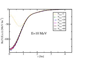
Figure 1: Real part of the radial (diagonal) optical potential in the neutron $s$-wave at $E=10$ MeV as a function of ${N_{\rm lanc}}$ the number of Lanczos iteration. Calculations were performed with $N_{\rm max}=10$ and 50 discretized Berggren shells for the neutron $s_{1/2}$ partial wave.

Results should be independent on the choice of the contour $L^{+}$ in the complex momentum plane as long as its discretization is adequate for the infrared scales under consideration Furnstahl et al. (2012). Figure 3 shows the real part of the radial (diagonal) neutron $s$-wave potential at $E=1$ and $E=10$ MeV using two contours ${L^{+}_{1}}$ and ${L^{+}_{2}}$. Both contours, shown in Fig. 2, are defined by two segments $[k_{a},k_{b}]$ and $[k_{b},k_{c}]$ located on the fourth quadrant of the complex momentum plane where $k_{a}$ is taken as the origin. For the contour $L^{+}_{1}$, the segment $[k_{a},k_{b}]$ has a norm of ${\rm 0.4~{}fm^{-1}}$, with an argument equal to $-\pi/4$ and $[k_{b},k_{c}]$ is a horizontal segment with $\rm{Re(k_{c})=4~{}fm^{-1}}$. For the contour $L^{+}_{2}$, the segment $[k_{a},k_{b}]$ has a norm of ${\rm 0.2~{}fm^{-1}}$ and an angle equal to $-\pi/5$ and $[k_{b},k_{c}]$ is a horizontal segment with $\rm{Re(k_{c})=4~{}fm^{-1}}$. We take 10 and 50 points on each segments for $L^{+}_{1}$, whereas we take 5 and 45 points for the discretization of $L^{+}_{2}$, respectively. Figure 3 shows that the results are practically independent of the choice of the contour.

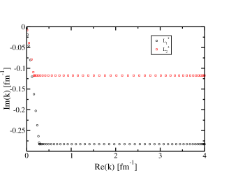
Figure 2: k-plane contours $L^{+}_{1},L^{+}_{2}$ used in the calculation of the $s$-wave optical potential in Fig. 3.

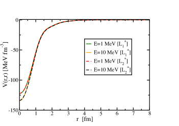
Figure 3: Real part of the radial (diagonal) optical potential in the neutron $s$-wave at $E=1$ and $E=10$ MeV using two different contours $L^{+}_{1},L^{+}_{2}$ for the single-particle neutron $s_{1/2}$ shells, in a model space with $N_{\rm max}=10$.

In Fig. 4, we illustrate the numerical stability of our approach as $\eta\rightarrow 0$. We show the imaginary part of the (diagonal) $s$-wave Green’s function $G_{s_{1/2}}(r,E)\equiv G_{s_{1/2}}(r,r,E)$ using (i) a complex and (ii) real set of HF orbitals for the $s_{1/2}$ neutron shells. While the shown results are for $r=2.4$ fm, we note that the qualitative behavior is independent of the value of $r$. As expected (see Sec. II.4), for $\eta$ values significantly larger than zero, both bases give the same results. Let us first consider the real HF basis, corresponding to the dashed lines in Fig.  4. For $\eta=2$ MeV the results are smooth but, as $\eta$ decreases, the considerable oscillations appear, and for $\eta\sim 0$ peaks with widths proportional to $\eta$ start to appear near the Green’s function poles, at real energies. If instead we use a complex single-particle basis (solid lines in Fig.  4) no such instability occurs as $\eta\rightarrow 0$.

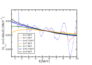
Figure 4: Imaginary part of the neutron s-wave Green’s function $G_{s1/2}(r,E)$ at $r=2.4$ fm (see text for details). The dashed lines correspond to calculations with a real HF basis whereas the full lines were obtained using a complex contour. Calculations were performed with ${N_{\rm max}=10}$ and 50 discretized shells in the ${s_{1/2}}$ partial wave.

Next, we show in Fig. 5, the convergence of the real part of the (diagonal) the $s$-wave optical potential as the size of the model space increases from ${N_{\rm max}=8}$ to $14$. Results are shown for $E=10$ MeV and, in all cases, 50 discretized shells are used for the Berggren basis in the $s$-wave, and $\eta=0$. For $N_{max}=10$ and $E=10$ MeV, the results agree with those shown in Fig. 3. Convergence is achieved for $N_{\rm max}=14$ for $r\geq 1$ fm. For small values of $r$, the optical potential depends on $N_{\rm max}$. This is understandable because short-range physics gets better resolved as the model space increases., and thus convergence becomes harder. Again we note that in this region the scattering wave function $u(r)\propto r$ and the dependence of the potential on ${N_{\rm max}}$ does not impact observables. To demonstrate this point, Fig. 6 shows the integrated quantity

$$V_{\rm int}(r)\equiv r\int dr^{\prime}r^{\prime}V(r,r^{\prime})u(r^{\prime})=V^{\rm eq}(r)u(r).$$ (31)

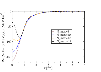
Figure 5: Real part of the diagonal optical potential in the neutron $s$-wave at $E=10$ MeV. Results are shown for at ${N_{\rm max}=8-14}$ and 50 discretized shells in the $s_{1/2}$ partial wave

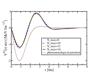
Figure 6: Real part of $V_{\rm int}(r)$ in the neutron s-wave at E=10 MeV. Results are shown for at ${N_{\rm max}=8-14}$. For illustration purpose, we also show the results obtained with the phenomenological potential from Ref. Capote et al. (2009).

The potential $V_{\rm int}(r)$ can be viewed as the local equivalent potential $V^{\rm eq}(r)$ multiplied by the scattering wave function, and corresponds to the source term in the one-body optical-model-type Schrödinger equation. The variations of the optical potential with the model space for small values of $r$ do not impact the behavior of $V_{\rm int}(r)$. For illustration, Fig. 6 also shows a result for $V_{\rm int}(r)$ obtained using a phenomenological potential based on a Woods-Saxon form factor Capote et al. (2009).

So far, we have only presented results for the diagonal part of the optical potential. Figure 7 shows a contour plot for the nonlocal neutron $s$-wave optical potential. Introducing the relative coordinate $r_{\rm rel}=r-r^{\prime}$ and the center-of-mass coordinate $R=(r+r^{\prime})/2$ we plot the optical potential as a function of $r_{\rm rel}$ at fixed $R=1$ fm in Fig. 8. We can see that the full width at half maximum is about 2.2 fm. Clearly, this potential is very different from a model of a Dirac $delta$ function in $r_{\rm rel}$ and exemplifies the degree of nonlocality which is predicted microscopically. We note that due to the non-Hermitian nature of the coupled-cluster method, the potential $V(r,r^{\prime})$ is slightly non-symmetric in $r$ and $r^{\prime}$, and as a consequence $V(R,r_{\rm rel})$ is not quite an even function of $r_{\rm rel}$. In Figs. 7, and 8 the energy is $E=10$ MeV and results were obtained for ${N_{\rm max}=14}$ and 50 discretized shells for the $s$-wave along a contour in the complex plane.

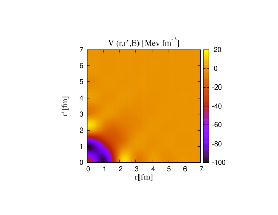
Figure 7: Contour plot of the real part of the neutron s-wave potential $V(r,r^{\prime},E)$ for ${N_{\rm max}=14}$ and 50 discretized $s$-wave shells at $E=10$ MeV.

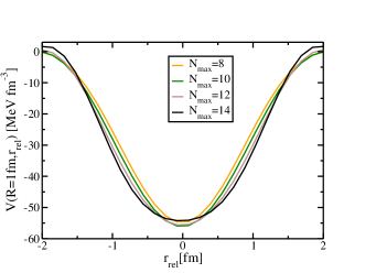
Figure 8: Neutron $s$-wave optical potential at E=10 MeV plotted as $V(R+r_{\rm rel}/2,R-r_{\rm rel}/2)$ at fixed $R=1/2$ fm. Here $N_{max}=14$ and 50 discretized $s$-wave shells are included in the single-particle basis.

Calculations of the optical potential in other partial waves follow along the same lines. For illustration, we show a contour plot of the ${d_{3/2}}$-wave potential in Fig. 9. Results are shown for $E=10$ MeV at ${N_{\rm max}=14}$ and 50 discretized shells for the $d_{3/2}$-wave along a complex contour. As in other cases, we take the limiting value $\eta=0$.

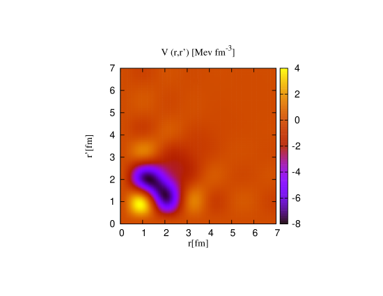
Figure 9: Contour plot of the real part of the neutron $d_{3/2}$-wave potential for ${N_{\rm max}=14}$ at $E=10$ MeV.

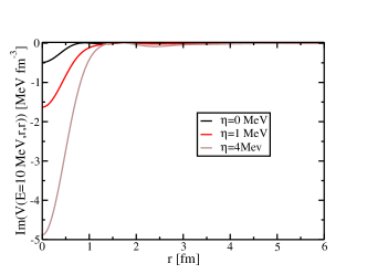
Figure 10: Imaginary part of the radial (diagonal) optical potential in the neutron $s$-wave at $E=10$ MeV. Calculations were performed at ${N_{\rm max}=10}$ with 50 $s_{1/2}$ discretized shells. Results are shown for several values of $\eta$.

We finally turn to the imaginary part of the optical potential. The imaginary part describes the loss of flux due to inelastic processes. For most nuclei, and particularly for heavier systems, there are many compound-nucleus resonances above the particle threshold, and absorption is known to be significant. Our results for the imaginary part of the potential, along the diagonal $r=r^{\prime}$ are shown in Fig. 10 for the neutron $s_{1/2}$ wave at $E=10$ MeV. The model space consists of $N_{max}=10$ and 50 discretized shells for the s-wave. We consider various values of $\eta$. In the limit $\eta=0$, the imaginary part of the potential is very small, and this is true for the whole range of energies up to $E=10$ MeV. As one can see in Fig. 10, as $\eta$ decreases to zero, the imaginary part also decreases and becomes very small for $\eta=0$. We observed the same qualitative behavior for all other considered partial wave, up to $d_{5/2}$, a result that does not change when the model space increases.

To further illustrate our difficulties with the imaginary part, we plot in Fig. 11 the imaginary volume integral $J^{l}_{W}$

$$J^{l}_{W}=4\pi\int drr^{2}\int drr^{\prime 2}{\rm Im}\Sigma^{\prime}_{l}(r,r^{\prime};E)$$ (32)

for the optical potential in the $s$-wave, taking a model space with $N_{\rm max}=14$ and 50 discretized s-waves.

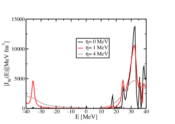
Figure 11: Neutron $s$-wave imaginary volume integral $J_{W}(E)$ for several values of $\eta$. Calculations were performed at $N_{\rm max}=14$ with 50 discretized $s_{1/2}$ shells.

In order to understand these results, we recall that the compound states that contribute to the flux removal from the elastic channel consist of a high number of particle-hole excitations and are usually described by stochastic approaches Mitchell et al. (2010). However, the coupled-cluster approach to the optical potential presented in this paper employs only $1p$-$1h$ and $2p$-$2h$ excitations and is thus limited to absorption on resonant states that are dominated by $1p$-$1h$ excitations. In our example of scattering off ¹⁶O, its $J^{\pi}=3^{-}$ state (at about 6 MeV of excitation energy) is thought to be of $1p$-$1h$ structure. With the NNLO_opt interaction, we computed this state using EOM-CCSD and found it at about 10 MeV of excitation. Another relevant excited state in ¹⁶O is the first excited $0^{+}$ state also at $\approx 6$ MeV, which is known to have a strong $4p-4h$ configuration. In our coupled cluster calculations this state is above $10$ MeV. In fact, there are no other excited states below 10 MeV. In general, positive parity states of ¹⁶O are dominated by $2p$-$2h$ excitations, and are therefore not well described in EOM-CCSD. Thus, from this analysis, we conclude that it is not possible to produce significant absorption at low-energies for neutron scattering on ¹⁶O due to the employed low-order cluster truncations in our EOM-CCSD and PA/PR-EOM CCSD approximations.

One path forward is to introduce a phenomenological and energy dependent width in the Green’s function, to account for higher-order correlations such as $3p$-$2h$ and $2p$-$3h$ not included in PA/PR-EOM CCSD Dickhoff et al. (2016). As shown in Fig.10, this will increase the absorption at lower energies. This would also allow to account for collective states which may exist in nature and which cannot be reproduced in the coupled cluster approach at the CCSD level.

Finally we show, in Fig. 12, the neutron elastic scattering phase shift obtained with the optical potential in the $s$ and $d$ partial waves, as a function of the model space . We want to emphasize here that calculations for higher partial waves proceed similarly and are straightforward. We find that, for $N_{\rm max}=14$ all calculated phase shifts have converged (all calculations here are done with 50 discretized shells). The sharp rise of the phase shift in the $d_{3/2}$ partial wave is the standard signature of the resonance $J^{\pi}=3/2^{+}$ in ¹⁷O, which is numerically predicted to be at $E=2.26-i0.12$ MeV from our PA-EOM CCSD calculations (see Table 1).

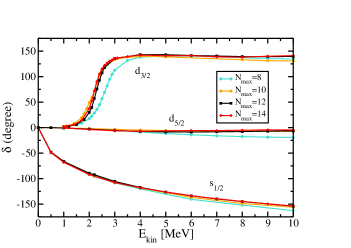
Figure 12: Elastic-scattering phase shifts in the neutron $s$ and $d$ waves as a function of $N_{\rm max}$. In all cases 50 discretized Berggren shells are included.

IV Conclusions

We constructed microscopic nuclear optical potentials by combining the Green’s function approach with the coupled-cluster method. For the computation of the Green’s function, we used an analytical continuation in the complex energy plane, based on a Berggren basis. Using the Lanczos method, we expressed the Green’s function as a continued fraction. The computational cost of a single Lanczos iteration is similar to that of a PA-EOM-CCSD calculation, i.e. polynomial in system size, and thus affordable. The convergence with the number of Lanczos iterations was demonstrated. The Dyson equation was then inverted to obtain the optical potential.

In the coupled-cluster singles and doubles approximation, the optical potential and the neutron elastic scattering phase shifts on ${}^{16}{\rm O}$ converge well with respect to the size of the single-particle basis, for the low partial waves. The predicted optical potential has a strong nonlocality that is not Gaussian. In addition, we found an almost vanishing imaginary part of the potential for scattering energies below 10 MeV. This lack of an absorptive component was attributed to neglected higher-order correlations in the employed coupled-cluster methods.

In the future, we plan to update the NN force currently used, to one that is able to reproduce charge radii of heavier systems. We also plan to include three-nucleon forces in the coupled-cluster calculations of the Green’s functions, as well as higher-order correlations in the employed coupled-cluster methods. We expect this will produce an increase in the imaginary part of the derived optical potential. Once these improvements are in place, this work can be extended to other systems (the limitations being the computational cost associated with the CC calculations) and to other reaction channels such as transfer, capture, breakup and charge-exchange. Systematic studies involving heavier nuclei and consistent calculations along isotopic chains will provide critical information on how to extrapolate the optical potential to unknown regions of the nuclear chart.