Strong approximations for the $p$-fold integrated empirical process
with applications to statistical tests

Abstract

The main purpose of this paper is to investigate the strong approximation of the $p$-fold integrated empirical process, $p$ being a fixed positive integer. More precisely, we obtain the exact rate of the approximations by a sequence of weighted Brownian bridges and a weighted Kiefer process. Our arguments are based in part on the Komlós et al. (1975)’s results. We obtain an exponential bound for the tail probability of the weighted approximation to the $p$-fold integrated empirical process. Applications include the two-sample testing procedures together with the change-point problems. We also consider the strong approximation of integrated empirical processes when the parameters are estimated. We study the behavior of the self-intersection local time of the partial sum process representation of integrated empirical processes. Finally, simulation results are provided to illustrate the finite sample performance of the proposed statistical tests based on the integrated empirical processes.
Key words: Integrated empirical process; Brownian bridge; Kiefer process; Rates of convergence; Local time; Two-sample problem; Hypothesis testing; Goodness-of-fit; Change-point.
AMS Classifications: primary: 62G30; 62G20; 60F17; secondary: 62F03; 62F12; 60F15.

1 Introduction

Let $F=\{F(t),t\in\mathbb{R}\}$ be a continuous distribution function [d.f.] and denote by $Q=\{Q(u),u\in[0,1]\}$ the usual quantile function (generalized inverse) pertaining to $F$ defined as

$$Q(u):=\inf\{t\in\mathbb{R}:F(t)\geq u\}\quad\text{for}\quad u\in(0,1),$$

$$Q(0):=\lim_{u\downarrow 0}Q(u)\quad\text{and}\quad Q(1):=\lim_{u\uparrow 1}Q(u).$$

The function $Q$ is strictly increasing and we have $F(Q(u))=u$ for any $u\in[0,1]$. We denote the sets $\{0,1,2,\ldots\}$ and $\{1,2,\ldots\}$ respectively by $\mathbb{N}$ and $\mathbb{N}^{*}$. Consider now a sequence of independent, identically distributed [i.i.d.] random variables [r.v.’s] $\{U_{i}:i\in\mathbb{N}^{*}\}$ uniformly distributed on $[0,1]$ and, for each $i\in\mathbb{N}^{*}$, set $X_{i}:=Q(U_{i})$. The sequence $\{X_{i}:i\in\mathbb{N}^{*}\}$ consists of i.i.d. r.v.’s with d.f. $F$: $F(t)=\mathbb{P}\{X_{1}\leq t\}$ for $t\in\mathbb{R}$ (cf., e.g., Shorack and Wellner (1986), p. 3 and the references therein). Moreover, we conversely have $U_{i}=F(X_{i})$.

For each $n\in\mathbb{N}^{*}$, let $\mathbb{F}_{n}$ and $\mathbb{U}_{n}$ be the empirical d.f.’s based upon the respective samples $X_{1},\ldots,X_{n}$ and $U_{1},\ldots,U_{n}$ defined by

$$\mathbb{F}_{n}(t) :=\frac{1}{n}\#\{i\in\{1,\dots,n\}:X_{i}\leq t\}=\frac{1}{n}\sum_{i=1}^{n}\mathbbm{1}_{\{X_{i}\leq t\}}\quad\text{for}\quad t\in\mathbb{R},$$

$$\mathbb{U}_{n}(u) :=\frac{1}{n}\#\{i\in\{1,\dots,n\}:U_{i}\leq u\}=\frac{1}{n}\sum_{i=1}^{n}\mathbbm{1}_{\{U_{i}\leq u\}}\quad\text{for}\quad u\in[0,1],$$

where $\#$ denotes cardinality. For each $n\in\mathbb{N}^{*}$, we introduce the empirical process $\alpha_{n}$ and the uniform empirical process $\beta_{n}$ defined by

$$\alpha_{n}(t) :=\sqrt{n}\,(\mathbb{F}_{n}(t)-F(t))\quad\text{for}\quad t\in\mathbb{R},$$ (1.1)

$$\beta_{n}(u) :=\sqrt{n}\left(\mathbb{U}_{n}(u)-u\right)\quad\text{for}\quad u\in[0,1].$$ (1.2)

We have of course the usual relations between the empirical process and uniform empirical process:

$$\alpha_{n}(t) =\beta_{n}(F(t))\quad\text{for}\quad t\in\mathbb{R},\,n\in\mathbb{N}^{*},$$ (1.3)

$$\beta_{n}(u) =\alpha_{n}(Q(u))\quad\text{for}\quad u\in\mathbb{[}0,1],\,n\in\mathbb{N}^{*}.$$ (1.4)

In this paper, we consider integrated empirical d.f.’s based upon the samples $X_{1},\ldots,X_{n}$ and $U_{1},\ldots,U_{n}$ together with the corresponding integrated empirical processes in the following sense.

Definition 1.1

We define the families of integrated d.f.’s and integrated empirical d.f.’s associated with the d.f. $F$, for any $p\in\mathbb{N}$, any $n\in\mathbb{N}^{*}$ and any $t\in\mathbb{R}$, as

$$F^{(0)}(t):=F(t),\quad\mathbb{F}_{n}^{(0)}(t):=\mathbb{F}_{n}(t),$$

$$F^{(1)}(t):=\int_{-\infty}^{t}F(s)\,dF(s),\quad\mathbb{F}_{n}^{(1)}(t):=\int_{-\infty}^{t}\mathbb{F}_{n}(s)\,d\mathbb{F}_{n}(s),$$

and for $p\geq 2$,

$$F^{(p)}(t):=\int_{-\infty}^{t}dF(s_{1})\int_{-\infty}^{s_{1}}\,dF(s_{2})\dots\int_{-\infty}^{s_{p-1}}F(s_{p})\,dF(s_{p}),$$

$$\mathbb{F}_{n}^{(p)}(t):=\int_{-\infty}^{t}\,d\mathbb{F}_{n}(s_{1})\int_{-\infty}^{s_{1}}\,d\mathbb{F}_{n}(s_{2})\dots\int_{-\infty}^{s_{p-1}}\mathbb{F}_{n}(s_{p})\,d\mathbb{F}_{n}(s_{p}),$$

together with the corresponding family of integrated empirical processes as

$$\alpha_{n}^{(p)}(t):=\sqrt{n}\left(\mathbb{F}_{n}^{(p)}(t)-F^{(p)}(t)\right)\!.$$ (1.5)

Notice that $F^{(p)}$ (resp. $\mathbb{F}_{n}^{(p)}$) is a kind of $p$-fold integral with respect to the measure $dF$ (resp. $d\mathbb{F}_{n}$). Hence, we will call $F^{(p)}$ (resp. $\mathbb{F}_{n}^{(p)}$, $\alpha_{n}^{(p)}$) throughout the paper $p$-fold integrated d.f. (resp. $p$-fold integrated empirical d.f., $p$-fold integrated empirical process). Finally, we define exactly in the same manner the $p$-fold integrated uniform empirical d.f. $\mathbb{U}_{n}^{(p)}$ and the $p$-fold integrated uniform empirical process $\beta_{n}^{(p)}$.

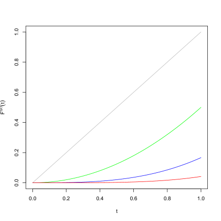
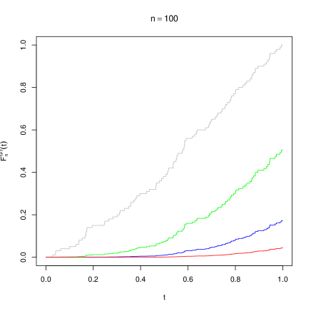
Figure 1: On the left: the theoretical functions $F^{(p)},p=0,1,2,3$; on the right: the empirical counterparts for the uniform distribution. (“–”: $\mathbb{F}_{n},F$ ), (“–”: $\mathbb{F}_{n}^{(1)},~{}~{}F^{(1)}$), (“–”: $\mathbb{F}_{n}^{(2)},~{}~{}F^{(2)}$), (“–”: $\mathbb{F}_{n}^{(3)},~{}~{}F^{(3)}$)

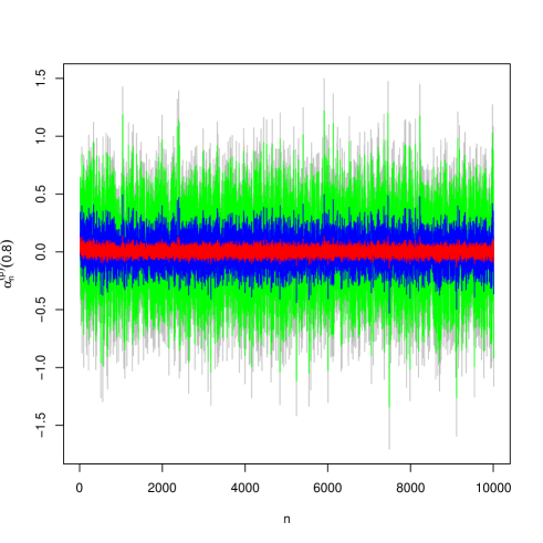
Figure 2: The uniform empirical processes for $p=0,1,2,3$ as functions of the sample size. (“–”: $\alpha_{n},$ ), (“–”: $\alpha^{(1)}_{n},$), (“–”: $\alpha_{n}^{(2)},$), (“–”: $\alpha_{n}^{(3)}$)

Below, we provide explicit expressions for $F^{(p)}$ and $\mathbb{F}_{n}^{(p)}$, the proof of which are postponed to Section 9.

Proposition 1.2

For each $p\in\mathbb{N}$, we explicitly have, with probability $1$,

$$F^{(p)}(t)=\frac{F(t)^{p+1}}{(p+1)!},\quad\mathbb{F}_{n}^{(p)}(t)=\frac{1}{n^{p+1}}{n\mathbb{F}_{n}(t)+p\choose p+1}\quad\text{for}\quad t\in\mathbb{R},\,n\in\mathbb{N}^{*}.$$ (1.6)

The particular case where $p=1$ has often been considered in the literature. Henze and Nikitin (2000, 2002) introduced and deeply investigated the goodness-of-fit testing procedures based on the integrated empirical process. Indeed, the asymptotic properties of their procedures, Kolmogorov-Smirnov, Cramér-von Mises and Watson-type statistics, can be derived from the limiting behavior of the integrated empirical process. Henze and Nikitin (2003) considered a two-sample testing procedure and focused on the approximate local Bahadur efficiencies of their statistical tests. It is noteworthy to point out that tests based on some integrated empirical processes turn out to be more efficient for certain distributions, we may refer at this point to Henze and Nikitin (2003, 2002, 2000). In Henze and Nikitin (2003), it is shown that the statistics based on the integrated empirical processes perform better the classical ones, under asymmetric alternatives. For instance, Kolmogorov-Smirnov test based on these integrated empiricals has maximal Bahadur efficiency if the underlying distribution is skew-Laplace. We mention also that in the paper Henze and Nikitin (2000) where a new approach to goodness-of-fit testing was proposed by using integrated empirical processes. In this paper, the authors have established that the integrated Kolmogorov- Smirnov test is locally Bahadur optimal for the logistic distribution and the statistic

$$\sqrt{n}\int_{\mathbb{R}}\left(\mathbb{F}_{n}^{(p)}(t)-F_{0}^{(p)}(t)\right)dF_{0}(t),~{}~{}\mbox{for}~{}~{}p=1,$$

turns out to be locally Bahadur optimal for the “root-logistic distribution”. In the paper by Henze and Nikitin (2002), one of the new tests is locally Bahadur optimal for the hyperbolic cosine distribution, we may refer to Theorem 6.1 therein for exact formulation. In Lachal (2001), another version of the $p$-fold integrated empirical process ($p\in\mathbb{N}^{*}$) was introduced. For the extension to the multivariate framework, we may refer to Jing and Wang (2006) and Jing and Yang (2007) where some projected integrated empirical processes for testing the equality of two multivariate distributions are considered. Inspired by the work of Henze and Nikitin (2003), Bouzebda and El Faouzi (2012) developed multivariate two-sample testing procedures based on the integrated empirical copula process that are extended to the $K$-sample problem in Bouzebda et al. (2011). Emphasis is placed on the explanation of the strong approximation methodology. The asymptotic behavior of weighted multivariate Cramér-von Mises-type statistics under contiguous alternatives was characterized by Bouzebda and Zari (2013). For more recent references, we refer to Durio and Nikitin (2016), Bouzebda (2016) and Alvarez-Andrade et al. (2017).

The main purpose of this paper is to investigate the strong approximation of the $p$-fold integrated empirical process. Next we use the obtained results for studying the asymptotic properties of statistical tests based on this process. We point out that strong approximations are quite useful and have received considerable attention in probability theory. Indeed, many well-known and important probability theorems can be considered as consequences of results about strong approximation of sequences of sums by corresponding Gaussian sequences.

We will first obtain an upper bound in probability for the distance between the $p$-fold integrated empirical process and a sequence of appropriate Brownian bridges (see Theorem 2.3). This is the key point of our study. From this, we will deduce a strong approximation of the $p$-fold integrated empirical process by this sequence of transformed Brownian bridges (see Corollary 2.5). As an application, we will derive the rates of convergence for the distribution of smooth functionals of each $p$-fold integrated empirical process (see Corollary 2.4). Moreover, we will deduce strong approximations for the Kolmogorov-Smirnov and Cramér-von Mises-type statistics associated with the $p$-fold integrated empirical processes (see Corollary 2.8).

Second, we will obtain a strong approximation of the $p$-fold integrated empirical process by a transformed Kiefer processes (see Theorem 2.6). This latter is of particular interest; indeed, for instance, any kind of law of the iterated logarithm which holds for the partial sums of Gaussian processes may then be transferred to the $p$-fold integrated empirical processes (see Corollary 2.7). We may refer to DasGupta (2008) (Chapter 12), Csörgő and Horváth (1993) (Chapter 3), Csörgő and Révész (1981) (Chapters 4-5) and Shorack and Wellner (1986) (Chapter 12) for expositions, details and references about this problem.

Third, we will apply our theoretical results to some statistical applications. More precisely, we will consider the famous two-sample and change-point problems for which we will develop procedures based on statistics involving $p$-fold integrated empirical distribution functions.

We refer to Csörgő and Hall (1984), Csörgő (2007) and Mason and Zhou (2012) for a survey of possible applications of the strong approximation and many references. There is a huge literature on the strong approximations and their applications. It is not the purpose of this paper to survey this extensive literature.

The layout of the article is as follows. In Section 2, we first present some strong approximation results for the $p$-fold integrated empirical process; our main tools are the results of Komlós et al. (1975). In section 3, we consider weighted approximations. Sections 4 and 5 are devoted to statistical applications, namely the two-sample and change-point problems respectively. In Section 6, we deal with the strong approximation of the $p$-fold integrated empirical process when parameters are estimated. Section 7 is concerned with the behavior of the self-intersection local time of the partial sum process representation of the $p$-fold integrated empirical process. In section 8, simulation results are performed in order to illustrate the finite sample performances of the proposed statistical tests for testing uniformity based on the integrated empirical processes. Finally, in the Appendix, we suggest some possible extensions of our work for further investigations.

To prevent from interrupting the flow of the presentation, all mathematical developments are postponed to Section 9.

2 Strong approximation

2.1 Some processes

First, we introduce some definitions and notations. Let $\mathbb{W}=\{\mathbb{W}(s):s\geq 0\}$ and $\mathbb{B}=\{\mathbb{B}(u):u\in[0,1]\}$ be the standard Wiener process and Brownian bridge, that is, the centered Gaussian processes with continuous sample paths, and covariance functions

$$\mathbb{E}(\mathbb{W}(s)\mathbb{W}(t))=s\wedge t\quad\text{for}\quad s,t\geq 0$$

and

$$\mathbb{E}(\mathbb{B}(u)\mathbb{B}(v))=u\wedge v-uv\quad\text{for}\quad u,v\in[0,1].$$

A Kiefer process $\mathbb{K}=\{\mathbb{K}(s,u):s\geq 0,u\in[0,1]\}$ is a two-parameters centered Gaussian process, with continuous sample paths, and covariance function

$$\mathbb{E}(\mathbb{K}(s,u)\mathbb{K}(t,v))=(s\wedge t)\,(u\wedge v-uv)\quad\text{for}\quad s,t\geq 0\quad\text{and}\quad u,v\in[0,1].$$

It satisfies the following distributional identities:

$$\left\{\mathbb{K}(s,u):u\in[0,1]\right\}\stackrel{{\scriptstyle\mathcal{L}}}{{=}}\left\{\sqrt{s}\,\mathbb{B}(u):u\in[0,1]\right\}\quad\text{for}\quad s\geq 0$$

and

$$\left\{\mathbb{K}(s,u):s\geq 0\right\}\stackrel{{\scriptstyle\mathcal{L}}}{{=}}\left\{\sqrt{u(1-u)}\,\mathbb{W}(s):s\geq 0\right\}\quad\text{for}\quad u\in[0,1],$$

where $\stackrel{{\scriptstyle\mathcal{L}}}{{=}}$ stands for the equality in distribution. The interested reader may refer to Csörgő and Révész (1981) for details on the Gaussian processes mentioned above.

2.2 Brownian approximation

It is well-known that the empirical uniform process $\{\beta_{n}:n\in\mathbb{N}^{*}\}$ converges to $\mathbb{B}$ in $D[0,1]$ (the space of all right-continuous real-valued functions defined on $[0,1]$ which have left-hand limits, equipped with the Skorohod topology; see, for details, Billingsley (1968)). The rate of convergence of this process to $\mathbb{B}$ is an important task in statistics as well as in probability that has been investigated by several authors. We can and will assume without loss of generality that all r.v.’s and processes introduced so far and later on in this paper can be defined on the same probability space (cf. Appendix 2 in Csörgő and Horváth (1993)).

In Csörgő et al. (1986), it was stated the following Brownian bridge approximation for $\{\beta_{n}:n\in\mathbb{N}^{*}\}$ (Formula (2.2)), along with a description of its proof with few details, which has been subsequently refined by Mason and van Zwet (1987) (Formula (2.1)).

Theorem A

On a suitable probability space, we may define the uniform empirical process $\{\beta_{n}:n\in\mathbb{N}^{*}\}$, in combination with a sequence of Brownian bridges $\{\mathbb{B}_{n}:n\in\mathbb{N}^{*}\}$, such that, for any $d,n\in\mathbb{N}^{*}$ satisfying $d\leq n$ and any positive number $x$,

$$\mathbb{P}\bigg{\{}\sup_{u\in[0,d/n]}\left|\beta_{n}(u)-\mathbb{B}_{n}(u)\right|\geq\frac{1}{\sqrt{n}}\,(c_{1}\log d+x)\bigg{\}}\leq c_{2}\,\exp(-c_{3}x)$$ (2.1)

where $c_{1}$, $c_{2}$ and $c_{3}$ are suitable absolute constants. The same inequality holds when replacing the interval $[0,d/n]$ by $[1-d/n,1]$. In particular, for $d=n$,

$$\mathbb{P}\bigg{\{}\sup_{u\in[0,1]}|\beta_{n}(u)-\mathbb{B}_{n}(u)|\geq\frac{1}{\sqrt{n}}\,(c_{1}\log n+x)\bigg{\}}\leq c_{2}\,\exp(-c_{3}x).$$ (2.2)

In (2.2), suitable explicit values for $c_{1},c_{2},c_{3}$ were exhibited by Bretagnolle and Massart (1989), Theorem 1: $c_{1}=12,c_{2}=2,c_{3}=1/6$. In his manuscript, Major (2000) details the original proof of (2.2). Chatterjee (2012) provided a new alternative approach for proving the famous KMT theorem.

Remark 2.1

In the sequel, the precise meaning of “suitable probability space” is that an independent sequence of Wiener processes, which is independent of the originally given sequence of i.i.d. r.v.’s, can be constructed on the assumed probability space. This is a technical requirement which allows the construction of the Gaussian processes displayed in our theorems, and which is not restrictive since one can expand the probability space to make it rich enough (see, e.g., Appendix 2 in Csörgő and Horváth (1993), de Acosta (1982), Csörgő and Révész (1981) and Lemma A1 in Berkes and Philipp (1979)). Throughout this paper, it will be assumed that the underlying probability spaces are suitable in this sense.

In the following theorem, we state the key point to access the strong Brownian approximation of the $p$-fold integrated uniform empirical process $\big{\{}\beta_{n}^{(p)}:n\in\mathbb{N}^{*}\big{\}}$. The following Theorem can be seen as a version of Csörgő et al. (1986) for iterated processes.

Theorem 2.2

Fix $p\in\mathbb{N}^{*}$. On a suitable probability space, we may define the $p$-fold integrated uniform empirical process $\big{\{}\beta_{n}^{(p)}:n\in\mathbb{N}^{*}\big{\}}$, in combination with a sequence of Brownian bridges $\{\mathbb{B}_{n}:n\in\mathbb{N}^{*}\}$, such that, for any $d,n\in\mathbb{N}^{*}$ satisfying $d\leq n$ and large enough $x$,

$$\mathbb{P}\bigg{\{}\sup_{u\in[0,d/n]}\left|\beta_{n}^{(p)}(u)-\mathbb{B}_{n}^{(p)}(u)\right|\geq\frac{1}{\sqrt{n}}\,(c_{1}\log d+x)\bigg{\}}\leq B_{p}\sum_{k=2}^{p+1}\exp\!\left(-C_{p}\,x^{2/k}n^{1-2/k}\right)$$ (2.3)

where $B_{p}$ and $C_{p}$ are positive constants depending on $p$, $c_{1}$ is the constant arising in (2.2) and, for each $n\in\mathbb{N}^{*}$, $\mathbb{B}_{n}^{(p)}$ is the process defined by

$$\mathbb{B}_{n}^{(p)}(u):=\frac{1}{p!}\,u^{p}\,\mathbb{B}_{n}(u)\quad\text{for}\quad u\in[0,1].$$

The same inequality holds when replacing the interval $[0,d/n]$ by $[1-d/n,1]$.

In particular, making $d=n$ in (2.3), we obtain the key estimate for the $p$-fold integrated empirical process $\big{\{}\alpha_{n}^{(p)}:n\in\mathbb{N}^{*}\big{\}}$ below.

Theorem 2.3

Fix $p\in\mathbb{N}^{*}$. On a suitable probability space, we may define the $p$-fold integrated empirical process $\{\alpha_{n}^{(p)}:n\in\mathbb{N}^{*}\}$, in combination with a sequence of Brownian bridges $\left\{\mathbb{B}_{n}:n\in\mathbb{N}^{*}\right\}$, such that, for large enough $x$ and all $n\in\mathbb{N}^{*}$,

$$\mathbb{P}\!\left\{\sup_{t\in\mathbb{R}}\left|\alpha_{n}^{(p)}(t)-\mathbb{B}_{n}^{(p)}(F(t))\right|\geq\frac{1}{\sqrt{n}}\,(c_{1}\log n+x)\right\}\leq B_{p}\sum_{k=2}^{p+1}\exp\!\left(-C_{p}\,x^{2/k}n^{1-2/k}\right)\!.$$ (2.4)

One of the immediate consequences of Theorem 2.3 is an upper bound for the convergence of distributions of smooth functionals of $\alpha_{n}^{(p)}$. Indeed, applying (2.4) with $x=c\log n$ for a suitable constant $c$ yields the result below. Notice that the following corollary is the analogous of the Corollary of Komlós et al. (1975) page 113. Let $\mathcal{D}(\mathbb{A})$ be the space of right-continuous real-valued functions defined on $\mathbb{A}$ which have left-hand limits, equipped with the Skorohod topology; refer to Billingsley (1968) for further details on this problem.

Corollary 2.4

Fix $p\in\mathbb{N}^{*}$. Let $\mathbb{B}$ be a Brownian bridge and $\mathbb{B}^{(p)}$ the process defined by

$$\mathbb{B}^{(p)}(u):=\frac{1}{p!}\,u^{p}\,\mathbb{B}(u)\quad\text{for}\quad u\in[0,1].$$

Let $\Phi(\cdot)$ be a functional defined on the space $\mathcal{D}(\mathbb{R})$, satisfying a Lipschitz condition

$$|\Phi(v)-\Phi(w)|\leq L\sup_{t\in\mathbb{R}}|v(t)-w(t)|.$$

Assume further that the distribution of the r.v. $\Phi\big{(}\mathbb{B}^{(p)}(F(\cdot))\big{)}$ has a bounded density. Then, as $n\to\infty$,

$$\sup_{x\in\mathbb{R}}\left|\mathbb{P}\!\left\{\Phi\big{(}\alpha_{n}^{(p)}(\cdot)\big{)}\leq x\right\}-\mathbb{P}\!\left\{\Phi\big{(}\mathbb{B}^{(p)}(F(\cdot))\big{)}\leq x\right\}\right|=\mathcal{O}\!\left(\frac{\log n}{\sqrt{n}}\right)\!.$$ (2.5)

For more comments on this kind of results, we may refer to Csörgő et al. (2000), Corollary 1.1 and p. 2459.

By applying (2.4) to $x=c^{\prime}\log n$ for a suitable constant $c^{\prime}$ and appealing to Borel-Cantelli lemma, one can obtain the following almost sure approximation of the process $\big{\{}\alpha_{n}^{(p)}:n\in\mathbb{N}^{*}\big{\}}$ based on a sequence of Brownian bridges.

Corollary 2.5

The following bound holds, with probability $1$, as $n\to\infty$:

$$\sup_{t\in\mathbb{R}}\left|\alpha_{n}^{(p)}(t)-\mathbb{B}_{n}^{(p)}(F(t))\right|=\mathcal{O}\!\left(\frac{\log n}{\sqrt{n}}\right)\!.$$ (2.6)

The next result yields an almost sure approximation for $\big{\{}\alpha_{n}^{(p)}:n\in\mathbb{N}^{*}\big{\}}$ based on a Kiefer process.

Theorem 2.6

On a suitable probability space, we may define the $p$-fold integrated empirical process $\big{\{}\alpha_{n}^{(p)}:n\in\mathbb{N}^{*}\big{\}}$, in combination with a Kiefer process $\{\mathbb{K}(s,u):s\geq 0,u\in[0,1]\}$, such that, with probability $1$, as $n\to\infty$,

$$\max_{1\leq k\leq n}\sup_{t\in\mathbb{R}}\left|\sqrt{k}\,\alpha_{k}^{(p)}(t)-\mathbb{K}^{(p)}(k,F(t))\right|=\mathcal{O}\!\left((\log n)^{2}\right)$$

where $\mathbb{K}^{(p)}$ is the process defined by

$$\mathbb{K}^{(p)}(s,u):=\frac{1}{p!}\,u^{p}\,\mathbb{K}(s,u)\quad\text{for}\quad s\geq 0,\,u\in[0,1].$$

Let us mention that the “extracted” Kiefer process $\{\mathbb{K}(n,u):n\in\mathbb{N}^{*},u\in[0,1]\}$ may be viewed as the partial sums process of a sequence of independent Brownian bridges $\left\{\mathbb{B}_{i}:i\in\mathbb{N}^{*}\right\}$:

$$\mathbb{K}(n,u)=\sum_{i=1}^{n}\mathbb{B}_{i}(u)\quad\text{for}\quad n\in\mathbb{N}^{*},\,u\in[0,1].$$

From Theorem 2.6, we deduce the following law of iterated logarithm (“a.s.” stands for “almost surely”).

Corollary 2.7

We have the following law of iterated logarithm for the $p$-fold integrated empirical process:

$$\limsup_{n\to\infty}\frac{\sup_{t\in\mathbb{R}}\big{|}\alpha_{n}^{(p)}(t)\big{|}}{\sqrt{\log\log n}}=\frac{(p+1/2)^{p+1/2}}{p!\,(p+1)^{p+1}}\quad\text{a.s.}$$ (2.7)

As a direct application of (2.6) and (2.7) to the problem of goodness-of-fit, for testing the null hypothesis

$$\mathcal{H}_{0}:F=F_{0},$$

we can use the following statistics: the $p$-fold integrated Kolmogorov-Smirnov statistic

$$\mathbf{S}_{n}^{(p)}:=\sup_{t\in\mathbb{R}}\left|\sqrt{n}\left(\mathbb{F}_{n}^{(p)}(t)-F_{0}^{(p)}(t)\right)\right|$$

as well as the $p$-fold integrated Cramér-von Mises statistic

$$\mathbf{T}_{n}^{(p)}:=n\int_{\mathbb{R}}\left(\mathbb{F}_{n}^{(p)}(t)-F_{0}^{(p)}(t)\right)^{\!2}dF_{0}(t).$$

Corollary 2.8

Under $\mathcal{H}_{0}$, with probability $1$, as $n\to\infty$, we have

$$\left|\mathbf{S}_{n}^{(p)}-\sup_{t\in\mathbb{R}}\big{|}\mathbb{B}_{n}^{(p)}(F_{0}(t))\big{|}\right| =\mathcal{O}\!\left(\frac{\log n}{\sqrt{n}}\right)\!,$$ (2.8)

$$\left|\mathbf{T}_{n}^{(p)}-\int_{\mathbb{R}}\big{[}\mathbb{B}_{n}^{(p)}(F_{0}(t))\big{]}^{2}\,dF_{0}(t)\right| =\mathcal{O}\!\left(\!\sqrt{\frac{\log\log n}{n}}\,\log n\right)\!.$$ (2.9)

We finish this part by pointing out the possibility of considering the statistics, for $r\geq 1$,

$$\omega_{n,p,r}=\sqrt{n}\left(\int_{\mathbb{R}}\left|\mathbb{F}_{n}^{(p)}(t)-F_{0}^{(p)}(t)\right|^{r}dF_{0}(t)\right)^{\!1/r}\!.$$

It is clear, however, that we have the following convergence in distribution as $n\to\infty$, under $\mathcal{H}_{0}$:

$$\sqrt{n}\left(\int_{\mathbb{R}}\left|\mathbb{F}_{n}^{(p)}(t)-F_{0}^{(p)}(t)\right|^{r}dF_{0}(t)\right)^{\!1/r}\longrightarrow\left(\int_{\mathbb{R}}\left|\mathbb{B}^{(p)}(F_{0}(t))\right|^{r}dF_{0}(t)\right)^{\!1/r}\!.$$

Denoting by $X_{(1)}\leq X_{(2)}\leq\cdots\leq X_{(n)}$ the order statistics of $X_{1},X_{2},\dots,X_{n}$, and putting $X_{(0)}=-\infty,X_{(n+1)}=+\infty$, straightforward manipulations of integrals yield the alternative representation, for $p=0$ and $r\geq 1$,

$$\omega_{n,0,r}= \;\frac{\sqrt{n}}{(r+1)^{1/r}}\left\{\sum_{i=1}^{n+1}\left[\left(F_{0}(X_{(i)})-\frac{i-1}{n}\right)\left|F_{0}(X_{(i)})-\frac{i-1}{n}\right|^{r}\right.\right.$$

$$-\left.\left.\left(F_{0}(X_{(i-1)})-\frac{i-1}{n}\right)\left|F_{0}(X_{(i-1)})-\frac{i-1}{n}\right|^{r}\right]\right\}^{1/r}.$$

In a future research, it would be of interest to deeply investigate such statistics.

3 Weighted approximations

In this part, we consider the weighted difference $\big{|}\beta_{n}^{(p)}(u)-\mathbb{B}_{n}^{(p)}(u)\big{|}/\big{(}u(1-u)\big{)}^{1/2-\nu}$ for a power $\nu\in[0,1/2)$. Since this quantity is not defined at $0$ and $1$, we will work with the supremum on an interval of the form $[d/n,1-d/n]$ for $d,n\in\mathbb{N}^{*}$ such that $d\leq n/2,{n\geq 2}$. The weighted approximations for the classical uniform empirical process were deeply studied in the papers by Csörgő et al. (1986), Haeusler and Mason (1999), Mason (1991), Mason (2001) and Mason and van Zwet (1987). For more details on the subject we may refer to Csörgő and Horváth (1993).

We state here the analogue of Theorem 1.2 of Mason (2001).

Theorem 3.1

Fix $p\in\mathbb{N}^{*}$. On a suitable probability space, we may define the $p$-fold uniform integrated empirical process $\big{\{}\beta_{n}^{(p)}:n\in\mathbb{N}^{*}\big{\}}$, in combination with a sequence of Brownian bridges $\left\{\mathbb{B}_{n}:n\in\mathbb{N}^{*}\right\}$ and a positive constant $C_{p}^{\prime}$, such that, for every $\nu\in[0,1/2)$, there exist a positive constant $B_{p,\nu}$ for which we have, for any $d,n\in\mathbb{N}^{*}$ satisfying $d\leq n/2$ and large enough $x$,

$$\mathbb{P}\bigg{\{}\sup_{u\in[d/n,1-d/n]}\frac{{n^{\nu}}\big{|}\beta_{n}^{(p)}(u)-\mathbb{B}_{n}^{(p)}(u)\big{|}}{\big{(}u(1-u)\big{)}^{{1/2-}\nu}}\geq x\bigg{\}}\leq B_{p,\nu}\sum_{k=2}^{p+1}\exp\!\left(-C_{p}^{\prime}\,x^{2/k}d^{2\nu/k}n^{1-(1+2\nu)/k}\right)\!.$$ (3.1)

This theorem may be proved by appealing to Theorem 2.2. Applying (3.1) with $x=c^{\prime\prime}(\log n)/n^{1/2-\nu}$ for a suitable constant $c^{\prime\prime}$ yields the result below.

Corollary 3.2

On the same probability space of Theorem 3.1, we have, for any $\nu\in[0,1/2)$ and any $d\in\mathbb{N}^{*}$, with probability $1$, as $n\to\infty$,

$$\sup_{u\in[d/n,1-d/n]}\frac{\big{|}\beta_{n}^{(p)}(u)-\mathbb{B}_{n}^{(p)}(u)\big{|}}{\big{(}u(1-u)\big{)}^{\nu}}=\mathcal{O}\!\left(\frac{\log n}{n^{1/2-\nu}}\right)\!.$$

By using Theorem 3.1 we have the following proposition.

Corollary 3.3

On the same probability space of Theorem 3.1, for all $0\leq\nu<1/2$ there exists a constant $\gamma>0$ such that

$$\sup_{n\geq 2}\mathbb{E}\left\{\exp\left(\gamma\sup_{u\in[1/n,1-1/n]}\frac{{n^{\nu}}\big{|}\beta_{n}^{(p)}(u)-\mathbb{B}_{n}^{(p)}(u)\big{|}}{\big{(}u(1-u)\big{)}^{{1/2-}\nu}}\right)\right\}<\infty.$$

4 The two-sample problem

For each $m,n\in\mathbb{N}^{*}$, let $X_{1},\ldots,X_{m}$ and $Y_{1},\ldots,Y_{n}$ be independent random samples from continuous d.f.’s $F$ and $G$, respectively, and let $\mathbb{F}_{m}^{(p)}$ and $\mathbb{G}_{n}^{(p)}$ denote their $p$-fold integrated empirical d.f.’s. Tests for the null hypothesis

$$\mathcal{H}_{0}^{\prime}:F=G,$$

can be based on the $p$-fold integrated two-sample empirical process defined, for each $m,n\in\mathbb{N}^{*}$, by

$$\boldsymbol{\xi}_{m,n}^{(p)}(t):=\sqrt{\frac{mn}{m+n}}\left(\mathbb{F}_{m}^{(p)}(t)-\mathbb{G}_{n}^{(p)}(t)\right)\quad\text{for}\quad t\in\mathbb{R}.$$

Actually, as in Bouzebda and El Faouzi (2012), we will more generally consider the following modified $p$-fold integrated two-sample empirical process (which includes the process $\boldsymbol{\xi}_{m,n}^{(p)}$). Fix a positive integer $q$ which will serve as a power. We define, for each $m,n\in\mathbb{N}^{*}$,

$$\boldsymbol{\xi}_{m,n}^{(p,q)}(t):=\sqrt{\frac{mn}{m+n}}\left[\left(\mathbb{F}_{m}^{(p)}(t)\right)^{\!q}-\left(\mathbb{G}_{n}^{(p)}(t)\right)^{\!q}\right]\quad\text{for}\quad t\in\mathbb{R}.$$

Set also, for any $m,n\in\mathbb{N}^{*}$,

$$\varphi(m,n):=\max\left(\frac{\log m}{\sqrt{m}},\frac{\log n}{\sqrt{n}}\right)\quad\text{and}\quad\phi(m,n):=\max\!\left(\sqrt{\frac{\log\log m}{m}}\,\log m,\sqrt{\frac{\log\log n}{n}}\,\log n\right)\!.$$

Reasonable statistics for testing $\mathcal{H}_{0}^{\prime}$ would be the modified $p$-fold integrated Kolmogorov-Smirnov statistic

$$\mathbf{S}_{m,n}^{(p,q)}:=\sup_{t\in\mathbb{R}}\big{|}\boldsymbol{\xi}_{m,n}^{(p,q)}(t)\big{|}$$

and the modified $p$-fold integrated Cramér-von Mises statistic

$$\mathbf{T}_{m,n}^{(p,q)}:=\int_{\mathbb{R}}\boldsymbol{\xi}_{m,n}^{(p,q)}(t)^{2}\,dF(t).$$

The following results are consequences of Corollary 2.5.

Corollary 4.1

On a suitable probability space, it is possible to define $\big{\{}\boldsymbol{\xi}_{m,n}^{(p,q)}:m,n\in\mathbb{N}^{*}\big{\}}$, jointly with two sequences of Brownian bridges $\big{\{}\mathbb{B}_{m}^{1}:m\in\mathbb{N}^{*}\big{\}}$ and $\big{\{}\mathbb{B}_{n}^{2}:n\in\mathbb{N}^{*}\big{\}}$, such that, under $\mathcal{H}_{0}^{\prime}$, with probability $1$, as $\min(m,n)\to\infty$,

$$\sup_{t\in\mathbb{R}}\left|\boldsymbol{\xi}_{m,n}^{(p,q)}(t)-\mathbb{B}_{m,n}^{(p,q)}(t)\right|=\mathcal{O}(\varphi(m,n)),$$

where, for each $m,n\in\mathbb{N}^{*}$, $\mathbb{B}_{m,n}^{(p,q)}$ is the Gaussian process defined by

$$\mathbb{B}_{m,n}^{(p,q)}(t):=\frac{(p+1)q}{(p+1)!^{q}}\,F(t)^{pq+q-1}\left(\sqrt{\frac{n}{m+n}}\,\mathbb{B}_{m}^{1}(F(t))-\sqrt{\frac{m}{m+n}}\,\mathbb{B}_{n}^{2}(F(t))\right)\quad\text{for}\quad t\in\mathbb{R}.$$

Corollary 4.2

Under $\mathcal{H}_{0}^{\prime}$, with probability $1$, as $\min(m,n)\to\infty$, we have

$$\left|\mathbf{S}_{m,n}^{(p,q)}-\sup_{t\in\mathbb{R}}\big{|}\mathbb{B}_{m,n}^{(p,q)}(t)\big{|}\right| =\mathcal{O}(\varphi(m,n)),$$

$$\left|\mathbf{T}_{m,n}^{(p,q)}-\int_{\mathbb{R}}\mathbb{B}_{m,n}^{(p,q)}(t)^{2}\,dF(t)\right| =\mathcal{O}(\phi(m,n)).$$

Remark 4.3

The family of statistics indexed by $q$ may be used to maximize the power of the statistical test for a specific alternative hypothesis as argued in Ahmad and Dorea (2001) in the case $p=1$.

Now, we fix a positive integer $K$ and we describe the more general $K$-sample problem. For each $k\in\{1,\dots,K\}$, we consider a setting made of independent observations $\big{\{}X_{i}^{k}:i\in\{1,\dots,n_{k}\}\big{\}}$ of a real-valued r.v. $X^{k}$. The d.f.’s of $X_{i}^{k}$, $i\in\{1,\ldots,n_{k}\}$, are denoted by $F^{k}$ and they are assumed to be continuous. We would like to test, $F_{0}$ being a fixed continuous d.f., the null hypothesis

$$\mathcal{H}_{0}^{K}:F^{1}=F^{2}=\dots=F^{K}=F_{0}.$$

For any $K$-tuple of positive integers $\boldsymbol{n}=(n_{1},\dots,n_{K})$, set $\boldsymbol{|n|}=\sum_{k=1}^{K}n_{k}$ and let

$$(Z_{1},\ldots,Z_{\boldsymbol{|n|}}):=\big{(}X_{1}^{1},\ldots,X_{n_{1}}^{1},X_{1}^{2},\ldots,X_{n_{2}}^{2},\ldots,X_{1}^{K},\ldots,X_{n_{K}}^{K}\big{)}$$

be the pooled sample of total size $\boldsymbol{|n|}$, $\mathbb{D}_{K,\boldsymbol{n}}^{(p)}$ be the $p$-fold integrated empirical d.f. based upon $Z_{1},\ldots,Z_{\boldsymbol{|n|}}$, and, for each $k\in\{1,\dots,K\}$, $\mathbb{F}_{n_{k}}^{k,(p)}$ be the $p$-fold integrated empirical d.f. based upon $X_{1}^{k},\ldots,X_{n_{k}}^{k}$. Of course, we have the following identity:

$$\mathbb{D}_{K,\boldsymbol{n}}^{(p)}=\frac{1}{\boldsymbol{|n|}}\sum_{k=1}^{K}n_{k}\,\mathbb{F}_{n_{k}}^{k,(p)}.$$ (4.1)

Next, we define the $p$-fold integrated $K$-sample empirical process in the following way: for any $K$-tuple $\boldsymbol{n}=(n_{1},\dots,n_{K})\in(\mathbb{N}^{*})^{K}$,

$$\boldsymbol{\xi}_{K,\boldsymbol{n}}^{(p)}(t):=\sum_{k=1}^{K}n_{k}\left(\mathbb{F}_{n_{k}}^{k,(p)}(t)-\mathbb{D}_{K,\boldsymbol{n}}^{(p)}(t)\right)^{\!2}\quad\text{for}\quad t\in\mathbb{R}.$$

Obvious candidates for testing Hypothesis $\mathcal{H}_{0}^{K}$ are the $p$-fold integrated $K$-sample Kolmogorov-Smirnov statistic

$$\mathbf{S}_{K,\boldsymbol{n}}^{(p)}:=\sup_{t\in\mathbb{R}}\boldsymbol{\xi}_{K,\boldsymbol{n}}^{(p)}(t)$$

and the $p$-fold integrated $K$-sample Cramér-von Mises functional (the usual square being included in the definition of $\boldsymbol{\xi}_{K,\boldsymbol{n}}^{(p)}$)

$$\mathbf{T}_{K,\boldsymbol{n}}^{(p)}:=\int_{\mathbb{R}}\boldsymbol{\xi}_{K,\boldsymbol{n}}^{(p)}(t)\,dF_{0}(t).$$

Set

$$\phi_{K}(\boldsymbol{n}):=\max_{1\leq k\leq K}\left\{\sqrt{\frac{\log\log n_{k}}{n_{k}}}\,\log n_{k}\right\}\!.$$

As a consequence of Corollary 2.5 and by using similar arguments to those used in Bouzebda et al. (2011), we obtain the following results.

Theorem 4.4

On a suitable probability space, it is possible to define $\big{\{}\boldsymbol{\xi}_{K,\boldsymbol{n}}^{(p)}:\boldsymbol{n}\in(\mathbb{N}^{*})^{K}\big{\}}$, jointly with $K$ sequences of Brownian bridges $\big{\{}\mathbb{B}_{m}^{k}:m\in\mathbb{N}^{*}\big{\}}$, $k\in\{1,\dots,K\}$, such that, under $\mathcal{H}_{0}^{K}$, with probability $1$, for $\boldsymbol{n}=(n_{1},\dots,n_{K})$ such that $\min_{1\leq k\leq K}n_{k}\to\infty$,

$$\sup_{t\in\mathbb{R}}\left|\boldsymbol{\xi}_{K,\boldsymbol{n}}^{(p)}(t)-\mathbb{B}_{K,\boldsymbol{n}}^{(p)}(t)\right|=\mathcal{O}\big{(}\phi_{K}(\boldsymbol{n})\big{)},$$

where, for each $\boldsymbol{n}=(n_{1},\dots,n_{K})\in(\mathbb{N}^{*})^{K}$, $\mathbb{B}_{K,\boldsymbol{n}}^{(p)}$ is the process defined by

$$\mathbb{B}_{K,\boldsymbol{n}}^{(p)}(t):=\frac{F_{0}(t)^{2p}}{p!^{2}}\!\left[\sum_{k=1}^{K}\mathbb{B}_{n_{k}}^{k}\!\big{(}F_{0}(t)\big{)}^{2}-\left(\sum_{k=1}^{K}\sqrt{\frac{n_{k}}{\boldsymbol{|n|}}}\,\mathbb{B}_{n_{k}}^{k}\!\big{(}F_{0}(t)\big{)}\right)^{\!\!2}\right]\quad\text{for}\quad t\in\mathbb{R}.$$

In the particular case $K=2$ (i.e. the two-sample problem), the corresponding settings are related to the previous ones according as

$$\boldsymbol{\xi}_{2,(n_{1},n_{2})}^{(p)}(t)=\left(\boldsymbol{\xi}_{n_{1},n_{2}}^{(p)}(t)\right)^{\!2},\quad\phi_{2}((n_{1},n_{2}))=\phi(n_{1},n_{2}),\quad\mathbf{S}_{2,(n_{1},n_{2})}^{(p)}=\left(\mathbf{S}_{n_{1},n_{2}}^{(p,1)}\right)^{\!2},\quad\mathbf{T}_{2,(n_{1},n_{2})}^{(p)}=\mathbf{T}_{n_{1},n_{2}}^{(p,1)}.$$

Notice that $\mathbb{B}_{K,\boldsymbol{n}}^{(p)}(t)\geq 0$ for any $t\in\mathbb{R}$ and $\boldsymbol{n}\in(\mathbb{N}^{*})^{K}$ as it is easily seen with the aid of the Cauchy-Schwarz inequality. For $K=2$, this process writes $\mathbb{B}_{2,(n_{1},n_{2})}^{(p)}=\left(\mathbb{B}_{n_{1},n_{2}}^{(p,1)}\right)^{\!2}$, this is the square of a Gaussian process.

The next result, which is an immediate consequence of the previous theorem (observe that $\mathbf{S}_{K,\boldsymbol{n}}^{(p)}$ and $\mathbf{T}_{K,\boldsymbol{n}}^{(p)}$ are bounded linear functionals of the process $\boldsymbol{\xi}_{K,\boldsymbol{n}}^{(p)}$), gives the limit null distributions of the statistics under consideration.

Corollary 4.5

Under $\mathcal{H}_{0}^{K}$, with probability $1$, for $\boldsymbol{n}=(n_{1},\dots,n_{K})$ such that $\min_{1\leq k\leq K}n_{k}\to\infty$, we have

$$\left|\mathbf{S}_{K,\boldsymbol{n}}^{(p)}-\sup_{t\in\mathbb{R}}\mathbb{B}_{K,\boldsymbol{n}}^{(p)}(t)\right| =\mathcal{O}\big{(}\phi_{K}(\boldsymbol{n})\big{)},$$

$$\left|\mathbf{T}_{K,\boldsymbol{n}}^{(p)}-\int_{\mathbb{R}}\mathbb{B}_{K,\boldsymbol{n}}^{(p)}(t)\,dF_{0}(t)\right| =\mathcal{O}\big{(}\phi_{K}(\boldsymbol{n})\big{)}.$$

5 The change-point problem

Here and elsewhere, $\lfloor t\rfloor$ denotes the largest integer not exceeding $t$. In many practical applications, we assume the structural stability of statistical models and this fundamental assumption needs to be tested before it can be applied. This is called the analysis of structural breaks, or change-points, which has led to the development of a variety of theoretical and practical results. For good sources of references to research literature in this area along with statistical applications, the reader may consult Brodsky and Darkhovsky (1993), Csörgő and Horváth (1997) and Chen and Gupta (2000). For recent references on the subject we may refer, among many others, to Bouzebda (2012), Aue and Horváth (2013), Chan et al. (2013), Horváth and Rice (2014), Alvarez-Andrade and Bouzebda (2014) and Bouzebda (2014).

In this section, we deal with testing changes in d.f.’s for a sequence of independent real-valued r.v.’s $X_{1},\ldots,X_{n}$. The corresponding null hypothesis that we want to test is

$$\mathcal{H}_{0}^{\prime\prime}:X_{1},\ldots,X_{n}\text{~{}~{}have d.f.~{}~{}}F.$$

As frequently done, the behavior of the derived tests will be investigated under the alternative hypothesis of a single change-point

$$\mathcal{H}_{1}^{\prime\prime}:\exists~{}k^{*}\in\{1,\ldots,n-1\}\text{~{}~{}such that~{}~{}}X_{1},\ldots,X_{k^{*}}\text{~{}~{}have d.f.~{}~{}}F\text{~{}~{}and~{}~{}}X_{k^{*}+1},\ldots,X_{n}\text{~{}~{}have d.f.~{}~{}}G.$$

The d.f.’s $F$ and $G$ are assumed to be continuous. The critical integer $k^{*}$ can be written as $\lfloor ns\rfloor$ for a certain $s\in(0,1)$. Then, testing the null hypothesis $\mathcal{H}_{0}^{\prime\prime}$ can be based on functionals of the following process: set, for each $n\in\mathbb{N}^{*}$,

$$\widetilde{\alpha}_{n}^{(p)}(s,t):=\frac{\lfloor ns\rfloor(n-\lfloor ns\rfloor)}{n^{3/2}}\left(\mathbb{F}_{\lfloor ns\rfloor}^{(p)-}(t)-\mathbb{F}_{n-\lfloor ns\rfloor}^{(p)+}(t)\right)\quad\text{for}\quad s\in(0,1),\,t\in\mathbb{R},$$ (5.1)

where $\mathbb{F}_{k}^{(p)-}$ is the $p$-fold integrated empirical d.f. based upon the $k$ first observations while $\mathbb{F}_{n-k}^{(p)+}$ is that based upon the $(n-k)$ last ones. In (5.1) we extend the definition of $\mathbb{F}_{k}^{(p)-}$ and $\mathbb{F}_{k}^{(p)+}$ to the case where $k=0$ by setting $\mathbb{F}_{0}^{(p)-}=\mathbb{F}_{0}^{(p)+}=0$, so that $\widetilde{\alpha}_{n}^{(p)}(s,t)=0$ if $s\in(0,1/n)$.

We can define the r.v.’s $X_{1},\ldots,X_{\lfloor ns\rfloor}$ and $X_{\lfloor ns\rfloor+1},\ldots,X_{n}$ on a probability space on which we can simultaneously construct two Kiefer processes $\{\mathbb{K}_{1}(s,u):s\in\mathbb{R},u\in[0,1]\}$ and $\{\mathbb{K}_{2}(s,u):s\in\mathbb{R},u\in[0,1]\}$ such that the “restricted” processes $\{\mathbb{K}_{1}(s,u):s\in[1,n/2],u\in[0,1]\}$ and $\{\mathbb{K}_{2}(s,u):s\in[n/2,n],u\in[0,1]\}$ are independent. It turns out that a natural approximation of $\big{\{}\widetilde{\alpha}_{n}^{(p)}:n\in\mathbb{N}^{*}\big{\}}$ is given by the sequence of Gaussian processes $\Big{\{}\overset{\text{\tiny o}}{\mathbb{K}}\vphantom{K}_{n}^{(p)}(s,F(t)):s\in[0,1],t\in\mathbb{R},n\in\mathbb{N}^{*}\Big{\}}$ defined by

$$\overset{\text{\tiny o}}{\mathbb{K}}\vphantom{K}_{n}^{(p)}(s,u):=\frac{1}{p!}\,u^{p}\,\overset{\text{\tiny o}}{\mathbb{K}}_{n}(s,u)\quad\text{for}\quad s,u\in[0,1],\,n\in\mathbb{N}^{*},$$ (5.2)

where, for each $n\in\mathbb{N}^{*}$, $\overset{\text{\tiny o}}{\mathbb{K}}_{n}:=\big{\{}\overset{\text{\tiny o}}{\mathbb{K}}_{n}(s,u):s,u\in[0,1]\big{\}}$ is the Gaussian process defined by

$$\overset{\text{\tiny o}}{\mathbb{K}}_{n}(s,u):=\!\begin{cases}\frac{1}{\sqrt{n}}\big{[}\,\mathbb{K}_{2}(\lfloor ns\rfloor,u)-s(\mathbb{K}_{1}(\lfloor n/2\rfloor,u)+\mathbb{K}_{2}(\lfloor n/2\rfloor,u))\big{]}&\!\!\!\text{for }s\in\!\big{[}0,\frac{1}{2}\big{]},u\in[0,1],\\[4.30554pt] \frac{1}{\sqrt{n}}\big{[}\!-\mathbb{K}_{1}(\lfloor n(1-s)\rfloor,u)+(1-s)(\mathbb{K}_{1}(\lfloor n/2\rfloor,u)+\mathbb{K}_{2}(\lfloor n/2\rfloor,u))\big{]}&\!\!\!\text{for }s\in\!\big{[}\frac{1}{2},1\big{]},u\in[0,1].\end{cases}$$

More precisely, we have the following result.

Theorem 5.1

On a suitable probability space, it is possible to define $\big{\{}\widetilde{\alpha}_{n}^{(p)}:n\in\mathbb{N}^{*}\big{\}}$, jointly with a sequence of Gaussian processes $\Big{\{}\overset{\text{\rm\tiny o}}{\mathbb{K}}\vphantom{K}_{n}^{(p)}:n\in\mathbb{N}^{*}\Big{\}}$ as above, such that, under $\mathcal{H}_{0}^{\prime\prime}$, with probability $1$, as $n\to\infty$,

$$\sup_{s\in(0,1)}\sup_{t\in\mathbb{R}}\left|\widetilde{\alpha}_{n}^{(p)}(s,t)-\overset{\text{\rm\tiny o}}{\mathbb{K}}\vphantom{K}_{n}^{(p)}(s,F(t))\right|=\mathcal{O}\!\left(\frac{(\log n)^{2}}{\sqrt{n}}\right)\!.$$

According to Csörgő et al. (1997), a way to test change-point is to use the following statistics:

$$\sigma_{n}^{(p)}:=\sup_{s\in(0,1)}\sup_{t\in\mathbb{R}}\left|\widetilde{\alpha}_{n}^{(p)}(s,t)\right|.$$ (5.3)

The corollary below is a consequence of Theorem 5.1 which can be proved by following exactly the same lines of Alvarez-Andrade et al. (2017).

Corollary 5.2

If $\mathcal{H}_{0}^{\prime\prime}$ holds true, then we have the convergence in distribution, as $n\to\infty$,

$$\sigma_{n}^{(p)}\stackrel{{\scriptstyle\mathcal{L}}}{{\longrightarrow}}\sup_{s,u\in[0,1]}\left|\overset{\text{\rm\tiny o}}{\mathbb{K}}\vphantom{K}^{(p)}(s,u)\right|,$$

where $\overset{\text{\rm\tiny o}}{\mathbb{K}}\vphantom{K}^{(p)}=\big{\{}\overset{\text{\rm\tiny o}}{\mathbb{K}}\vphantom{K}^{(p)}(s,u):s,u\in[0,1]\big{\}}$ is a Gaussian process with mean zero and covariance

$$\mathbb{E}\!\left(\overset{\text{\rm\tiny o}}{\mathbb{K}}\vphantom{K}^{(p)}(s,u)\,\overset{\text{\rm\tiny o}}{\mathbb{K}}\vphantom{K}^{(p)}(s^{\prime},u^{\prime})\right)=\frac{1}{p!^{2}}\,u^{p}u^{\prime p}(u\wedge u^{\prime}-uu^{\prime})(s\wedge s^{\prime}-ss^{\prime}).$$

One has $\overset{\text{\tiny o}}{\mathbb{K}}\vphantom{K}^{(p)}(s,u)=\frac{1}{p!}\,u^{p}\,\overset{\text{\tiny o}}{\mathbb{K}}(s,u)$ where $\overset{\text{\tiny o}}{\mathbb{K}}$ is a tied-down Kiefer process. We refer to Csörgő and Horváth (1997) for more details on the process $\mathbb{K}^{(p)}$ in the case where $p=1$.

Actually, according to Csörgő et al. (1997), the most appropriate way to test change-point is to use the following weighted statistic:

$$\sigma_{n,w}^{(p)}:=\sup_{s\in(0,1)}\sup_{t\in\mathbb{R}}\frac{\left|\widetilde{\alpha}_{n}^{(p)}(s,t)\right|}{w\left(\lfloor ns\rfloor/n\right)}$$ (5.4)

where $w$ is a positive function defined on $(0,1)$, increasing in a neighborhood of zero and decreasing in a neighborhood of one satisfying the condition

$$I(w,\boldsymbol{\varepsilon}):=\int_{0}^{1}\exp\left(-\frac{\boldsymbol{\varepsilon}w^{2}(s)}{s(1-s)}\right)\,\frac{ds}{s(1-s)}<\infty$$

for some constant $\boldsymbol{\varepsilon}>0$. For a history and further applications of $I(w,\boldsymbol{\varepsilon})$, we refer to Csörgő and Horváth (1993), Chapter 4. From Szyszkowicz (1992), an example of such function $w$ is given by

$$w(t):=\left(t(1-t)\log\log\frac{1}{t(1-t)}\right)^{\!1/2}\quad\text{for}\quad t\in(0,1).$$

By using similar techniques to those which are developed in Csörgő and Horváth (1997), one may show that

$$\sigma_{n,w}^{(p)}\stackrel{{\scriptstyle\mathcal{L}}}{{\longrightarrow}}\sup_{s,u\in[0,1]}\frac{\left|\overset{\text{\rm\tiny o}}{\mathbb{K}}\vphantom{K}^{(p)}(s,u)\right|}{w(s)}.$$

For more details, we refer to Alvarez-Andrade and Bouzebda (2014).

Remark 5.3

As in Szyszkowicz (1994), we mention that the statistic given by (5.3) should be more powerful for detecting changes that occur in the middle, i.e., near $n/2$, where $k/n(1-k/n)$ reaches its maximum, than for the ones occurring near the end points. The advantage of using the weighted statistic defined in (5.4) is the detection of changes that occur near the end points, while retaining the sensitivity to possible changes in the middle as well.

We hope that the results presented in Sections 4 and 5 will be the prototypes of other various applications.

6 Strong approximation of the integrated empirical process when parameters are estimated

In this section, we are interested in the strong approximation of the integrated empirical process when parameters are estimated. Our approach is in the same spirit of Burke et al. (1979). Let us introduce, for each $n\in\mathbb{N}^{*}$, the $p$-fold integrated estimated empirical process $\widehat{\alpha}_{n}^{(p)}$:

$$\widehat{\alpha}_{n}^{(p)}(t):=\sqrt{n}\left(\mathbb{F}_{n}^{(p)}(t)-F^{(p)}\big{(}t,\widehat{\boldsymbol{\theta}}_{n}\big{)}\right)\quad\text{for}\quad t\in\mathbb{R},$$ (6.1)

where $\big{\{}\widehat{\boldsymbol{\theta}}_{n}:n\in\mathbb{N}^{*}\big{\}}$ is a sequence of estimators of a parameter $\boldsymbol{\theta}$ from a family of d.f.’s $\{F(t,\boldsymbol{\theta}):t\in\mathbb{R},\,\boldsymbol{\theta}\in\boldsymbol{\Theta}\}$ ($\boldsymbol{\Theta}$ being a subset of $\mathbb{R}^{d}$ and $d$ a fixed positive integer) related to a sequence of i.i.d. r.v.’s $\{X_{i}:i\in\mathbb{N}^{*}\}$. Let us mention that a general study of the weak convergence of the estimated empirical process was carried out by Durbin (1973). For a more recent reference, we may refer to Genz and Haeusler (2006) where the authors investigated the empirical processes with estimated parameters under auxiliary information and provided some results regarding the bootstrap in order to evaluate the limiting laws.

Let us introduce some notations.

1. The transpose of a vector $V$ of $\mathbb{R}^{d}$ will be denoted by $V^{\top}$.

2. The norm $\|\cdot\|$ on $\mathbb{R}^{d}$ is defined by

   $$\|(y_{1},\ldots,y_{d})\|:=\max_{1\leq i\leq d}|y_{i}|.$$

3. For a function $(t,\boldsymbol{\theta})\mapsto g(t,\boldsymbol{\theta})$ where $\boldsymbol{\theta}=(\theta_{1},\ldots,\theta_{d})\in\mathbb{R}^{d}$, $\nabla_{\boldsymbol{\theta}}g(t,\boldsymbol{\theta}_{0})$ denotes the vector in $\mathbb{R}^{d}$ of partial derivatives $\big{(}(\partial g/\partial\theta_{1})(t,\boldsymbol{\theta}),\ldots,(\partial g/\partial\theta_{d})(t,\boldsymbol{\theta}))\big{)}$ evaluated at $\boldsymbol{\theta}=\boldsymbol{\theta}_{0}$, and $\nabla_{\boldsymbol{\theta}}^{2}g(t,\boldsymbol{\theta})$ denotes the $d\times d$ matrix of second order partial derivatives $\big{(}(\partial^{2}g/\partial\theta_{i}\partial\theta_{j})(t,\boldsymbol{\theta}))\big{)}_{1\leq i,j\leq d}$.

4. For a vector-valued function $x\mapsto V(x)=(v_{1}(x),\dots,v_{d}(x))$ defined on $\mathbb{R}$, $\int V$ denotes the vector

   $$\left(\int_{\mathbb{R}}v_{1}(x_{1})\,dx_{1},\dots,\int_{\mathbb{R}}v_{d}(x_{d})\,dx_{d}\right).$$

Next, we write out the set of all conditions (those of Burke et al. (1979)) which we will use in the sequel.

1. The estimator $\widehat{\boldsymbol{\theta}}_{n}$ admits the following form: for each $n\in\mathbb{N}^{*}$,

   $$\sqrt{n}\left(\widehat{\boldsymbol{\theta}}_{n}-\boldsymbol{\theta}_{0}\right)=\frac{1}{\sqrt{n}}\sum_{i=1}^{n}l(X_{i},\boldsymbol{\theta}_{0})+\boldsymbol{\varepsilon}_{n},$$

   where $\boldsymbol{\theta}_{0}$ is the theoretical true value of $\boldsymbol{\theta}$, $l(\cdot,\boldsymbol{\theta}_{0})$ is a measurable $d$-dimensional vector-valued function, and $\boldsymbol{\varepsilon}_{n}$ converges to zero as $n\to\infty$ in a manner to be specified later on. Notice that

   $$\frac{1}{\sqrt{n}}\sum_{i=1}^{n}l(X_{i},\boldsymbol{\theta}_{0})=\sqrt{n}\int_{-\infty}^{\infty}l(s,\boldsymbol{\theta}_{0})\,d\mathbb{F}_{n}(s).$$

2. The mean value of $l(X_{i},\boldsymbol{\theta}_{0})$ vanishes:

   $$\mathbb{E}\!\left(l(X_{i},\boldsymbol{\theta}_{0})\right)=0.$$

3. The matrix $M(\boldsymbol{\theta}_{0}):=\mathbb{E}\!\left(l(X_{i},\boldsymbol{\theta}_{0})^{\top}l(X_{i},\boldsymbol{\theta}_{0})\right)$ is a finite nonnegative definite $d\times d$ matrix.

4. The vector-valued function $(t,\boldsymbol{\theta})\mapsto\nabla_{\boldsymbol{\theta}}F(t,\boldsymbol{\theta})$ is uniformly continuous in $t\in\mathbb{R}$ and $\boldsymbol{\theta}\in\mathbf{V}$, where $\mathbf{V}$ is the closure of a given neighborhood of $\boldsymbol{\theta}_{0}$.

5. Each component of the vector-valued function $t\mapsto l(t,\boldsymbol{\theta}_{0})$ is of bounded variation in $t$ on each finite interval of $\mathbb{R}$.

6. The vector-valued function $t\mapsto\nabla_{\boldsymbol{\theta}}F(t,\boldsymbol{\theta}_{0})$ is uniformly bounded in $t\in\mathbb{R}$, and the vector-valued function $(t,\boldsymbol{\theta})\mapsto\nabla^{2}_{\boldsymbol{\theta}}F(t,\boldsymbol{\theta})$ is uniformly bounded in $t\in\mathbb{R}$ and $\boldsymbol{\theta}\in\mathbf{V}$.

7. Set

   $$\ell(s,\boldsymbol{\theta}_{0}):=l\!\left(F^{-1}(s,\boldsymbol{\theta}_{0}),\boldsymbol{\theta}_{0}\right)\quad\text{for}\quad s\in(0,1)$$

   where

   $$F^{-1}(s,\boldsymbol{\theta}_{0})=\inf\{t\in\mathbb{R}:F(t,\boldsymbol{\theta}_{0})\geq s\}.$$

   The limiting relations below hold:

   $$\lim_{s\searrow 0}\sqrt{s\log\log(1/s)}\,\left\|\ell(s,\boldsymbol{\theta}_{0})\right\|=0$$

   and

   $$\lim_{s\nearrow 1}\sqrt{(1-s)\log\log[1/(1-s)]}\,\left\|\ell(s,\boldsymbol{\theta}_{0})\right\|=0,$$

8. Set

   $$\ell^{\prime}_{s}(s,\boldsymbol{\theta}_{0}):=\frac{\partial\ell}{\partial s}(s,\boldsymbol{\theta}_{0})\quad\text{for}\quad s\in(0,1).$$

   The partial derivative $\ell^{\prime}_{s}(s,\boldsymbol{\theta}_{0})$ exist for every $s\in(0,1)$ and the bounds below hold: there is a positive constant $C$ such that

   $$s\left\|\ell^{\prime}_{s}(s,\boldsymbol{\theta}_{0})\right\|\leq C\quad\text{for all }s\in\big{(}0,\textstyle{\frac{1}{2}}\big{)}$$

   and

   $$(1-s)\left\|\ell^{\prime}_{s}(s,\boldsymbol{\theta}_{0})\right\|\leq C\quad\text{for all }s\in\big{(}\textstyle{\frac{1}{2}},1\big{)}.$$

Now, we state an analogous result to Theorem 3.1 of Burke et al. (1979). For each $n\in\mathbb{N}^{*}$, let $\{G_{n}(t):t\in\mathbb{R}\}$ be the process defined by

$$G_{n}(t) :=\frac{1}{\sqrt{n}}\left(\mathbb{K}(n,F(t,\boldsymbol{\theta}_{0}))-\left(\int_{\mathbb{R}}l(s,\boldsymbol{\theta}_{0})\,d_{s}\mathbb{K}(n,F(s,\boldsymbol{\theta}_{0}))\right)\nabla_{\boldsymbol{\theta}}F(t,\boldsymbol{\theta}_{0})^{\top}\right)$$

$$=\frac{1}{\sqrt{n}}\left(\mathbb{K}(n,F(t,\boldsymbol{\theta}_{0}))-\mathbf{W}(n)\nabla_{\boldsymbol{\theta}}F(t,\boldsymbol{\theta}_{0})^{\top}\right)\quad\text{for}\quad t\in\mathbb{R},$$

where we set

$$\mathbf{W}(\tau):=\int_{\mathbb{R}}l(s,\boldsymbol{\theta}_{0})\,d_{s}\mathbb{K}(\tau,F(s,\boldsymbol{\theta}_{0}))\quad\text{for}\quad\tau\geq 0.$$

The process $\{\mathbf{W}(\tau):\tau\geq 0\}$ is a $d$-dimensional Brownian motion with a covariance matrix of rank that of $M(\boldsymbol{\theta}_{0})$. The estimated empirical process given by $\widehat{\alpha}_{n}^{(p)}(t)$ defined by (6.1) will be approximated by the sequence of processes $\big{\{}G_{n}^{(p)}:n\in\mathbb{N}^{*}\big{\}}$ defined by

$$G_{n}^{(p)}(t):=\frac{1}{p!}\,F(t,\boldsymbol{\theta}_{0})^{p}\,G_{n}(t)\quad\text{for}\quad t\in\mathbb{R},$$ (6.2)

as described in the next theorem. Set

$$\boldsymbol{\varepsilon}_{n}^{(p)}:=\sup_{t\in\mathbb{R}}\left|\widehat{\alpha}_{n}^{(p)}(t)-G_{n}^{(p)}(t)\right|\!.$$ (6.3)

Theorem 6.1

Suppose that the sequence of estimators $\big{\{}\widehat{\boldsymbol{\theta}}_{n}:n\in\mathbb{N}^{*}\big{\}}$ satisfies conditions (i), (ii) and (iii). Then, as $n\to\infty$,

1. $\boldsymbol{\varepsilon}_{n}^{(p)}\stackrel{{\scriptstyle\mathbb{P}}}{{\longrightarrow}}0$ if Conditions (iv), (v) hold and $\boldsymbol{\varepsilon}_{n}\stackrel{{\scriptstyle\mathbb{P}}}{{\longrightarrow}}0$;

2. $\boldsymbol{\varepsilon}_{n}^{(p)}\stackrel{{\scriptstyle\text{a.s.}}}{{\longrightarrow}}0$ if Conditions (vi)–(viii) hold and $\boldsymbol{\varepsilon}_{n}\stackrel{{\scriptstyle\text{a.s.}}}{{\longrightarrow}}0$;

3. $\boldsymbol{\varepsilon}_{n}^{(p)}=\mathcal{O}(\max(h(n),n^{-\boldsymbol{\epsilon}}))$ for some $\boldsymbol{\epsilon}>0$ if Conditions (vi)–(viii) hold and $\boldsymbol{\varepsilon}_{n}=\mathcal{O}(h(n))$ for some function $h$ satisfying $h(n)>0$ and $h(n)\to 0.$

The limiting Gaussian process $G_{n}^{(p)}$ of Theorem 6.1 depends crucially on $F$ and also on the true theoretical value $\boldsymbol{\theta}_{0}$. In general, Theorem 6.1 cannot be used to test the composite hypothesis :

$$F\in\{F(t,\boldsymbol{\theta}):t\in\mathbb{R},\boldsymbol{\theta}\in\boldsymbol{\Theta}\}.$$

In order to circumvent this problem, Burke et al. (1979) proposed an approximate solution, they introduce another process:

$$\widehat{G}_{n}(t):=\frac{1}{\sqrt{n}}\left(\mathbb{K}\big{(}n,F\big{(}t,\widehat{\boldsymbol{\theta}}_{n}\big{)}\big{)}-\mathbf{W}(n)\nabla_{\boldsymbol{\theta}}F\big{(}t,\widehat{\boldsymbol{\theta}}_{n}\big{)}^{\top}\right)\!.$$

Under some regularity conditions, Burke et al. (1979) show that (see Theorem 3.2 therein), as $n\to\infty$,

$$\sup_{t\in\mathbb{R}}\left|\widehat{G}_{n}(t)-G_{n}(t)\right|\stackrel{{\scriptstyle\mathbb{P}}}{{\longrightarrow}}0.$$

Setting $\widehat{G}_{n}^{(p)}(t):=\frac{1}{p!}\,F\big{(}t,\widehat{\boldsymbol{\theta}}_{n}\big{)}^{p}\,\widehat{G}_{n}(t)$, one can show that, as $n\to\infty$,

$$\sup_{t\in\mathbb{R}}\left|\widehat{G}_{n}^{(p)}(t)-G_{n}^{(p)}(t)\right|\stackrel{{\scriptstyle\mathbb{P}}}{{\longrightarrow}}0.$$ (6.4)

Consequently, we have, as $n\to\infty$,

$$\sup_{t\in\mathbb{R}}\left|\widehat{\alpha}_{n}^{(p)}(t)-\widehat{G}_{n}^{(p)}(t)\right|\stackrel{{\scriptstyle\mathbb{P}}}{{\longrightarrow}}0.$$

7 Local time of the integrated empirical process

In this section, we are mainly concerned with the behavior of the local time of the $p$-fold integrated empirical process. This behavior can be characterized by using a representation that expresses the integrated empirical process in terms of a partial sums process, see (7.1) below. Let us recall the definition of the process $\beta_{n}$ given in (1.2) and let us introduce the modified $p$-fold integrated uniform empirical process $\widetilde{\beta}_{n}^{(p)}$ defined, for each $n\in\mathbb{N}^{*}$, by

$$\widetilde{\beta}_{n}^{(p)}(u):= \;\int_{0}^{u}dv_{1}\int_{0}^{v_{1}}dv_{p-1}\dots\int_{0}^{v_{p-1}}\beta_{n}(v_{p})\,dv_{p}$$

$$= \;\frac{1}{(p-1)!}\int_{0}^{u}(u-v)^{p-1}\,\beta_{n}(v)\,dv\quad\text{for}\quad u\in[0,1].$$

In this part, we fo cus on the particular r.v. $\mathcal{A}_{n}^{(p)}:=\widetilde{\beta}_{n}^{(p)}(1)$. It is easily seen that the representation below holds:

$$\mathcal{A}_{n}^{(p)}=\sqrt{n}\Bigg{(}\frac{1}{n}\sum_{i=1}^{n}\frac{1}{p!}\left(1-U_{i}\right)^{p}-\frac{1}{(p+1)!}\Bigg{)}=\frac{S_{n}^{(p)}}{\sqrt{n}}$$

where $\big{\{}S_{n}^{(p)}:n\in\mathbb{N}^{*}\big{\}}$ is the following partial sums process where the summands are i.i.d. r.v.’s with mean zero:

$$S_{n}^{(p)}:=\frac{1}{p!}\sum_{i=1}^{n}\left(\left(1-U_{i}\right)^{p}-\frac{1}{p+1}\right)\!.$$ (7.1)

This is a random walk with continuously distributed jumps. In the particular case where $p=1$, we retrieve the representation provided by Henze and Nikitin (2002) p. 185, namely

$$\mathcal{A}_{n}^{(1)}=\frac{S_{n}^{(1)}}{\sqrt{n}}\quad\text{with}\quad S_{n}^{(1)}:=\sum_{i=1}^{n}\left(\frac{1}{2}-U_{i}\right)\!.$$

Notice that we are dealing with a sum of strongly non-lattice r.v.’s as, i.e., in p. 210 of Bass and Khoshnevisan (1993a). Indeed, we easily check that the characteristic function $\chi^{(p)}$ of the $\left(1-U_{i}\right)^{p}-1/(p+1)$’s, namely

$$\chi^{(p)}(z):=\int_{0}^{1}\exp(\mathrm{i}z(u^{p}-1/(p+1)))\,du=\frac{\exp(-\mathrm{i}z/(p+1))}{pz^{1/p}}\int_{0}^{z}\exp(\mathrm{i}v)\frac{dv}{v^{1-1/p}}$$

satisfies the conditions

$$\forall z\in\mathbb{R}^{*},\,\big{|}\chi^{(p)}(z)\big{|}<1\quad\text{and}\quad\limsup_{|z|\to\infty}\big{|}\chi^{(p)}(z)\big{|}<1.$$

Next, we fix a neighborhood $I$ of $0$, e.g., $I=[-1/2,1/2]$, and we define the local time

$$\lambda^{(p)}(x,n):=\sum_{i=1}^{n}\mathbbm{1}_{I}\big{(}S_{i}^{(p)}-x\big{)}\quad\text{for}\quad x\in\mathbb{R},\,n\in\mathbb{N}^{*}.$$ (7.2)

The local time $\lambda^{(p)}(x,n)$ represents the number of visits of the random walk $\big{\{}S_{n}^{(p)}:n\in\mathbb{N}^{*}\big{\}}$ in the neighborhood $x+I$ of $x$ up to discrete time $n$. Our aim is to obtain the rate of the approximation of the self-intersection local time

$$L_{n}^{(p)}(t):=\sum_{1\leq i<j\leq\lfloor nt\rfloor}\int_{\mathbb{R}}\mathbbm{1}_{I}\big{(}S_{i}^{(p)}-x\big{)}\,\mathbbm{1}_{I}\big{(}S_{j}^{(p)}-x\big{)}\,dx$$

by the integrated local time of some standard Wiener process. The quantity $L_{n}^{(p)}(t)$ enumerates in a certain manner the couples $(i,j)$ of distinct and ordered indices up to time $\lfloor nt\rfloor$ such that $S_{i}-S_{j}$ is less than the diameter of $I$.

To this aim, we recall that, if $\{\mathbb{W}(t):t\geq 0\}$ is the standard Wiener process with $\mathbb{W}(0)=0$, then its local time process $\{l(x,t):t\geq 0,x\in\mathbb{R}\}$ is defined as

$$l(x,t):=\lim_{\boldsymbol{\varepsilon}\searrow 0}\frac{1}{2\boldsymbol{\varepsilon}}\int_{0}^{t}\mathbbm{1}_{\left\{x-\boldsymbol{\varepsilon}<\mathbb{W}(s)<x+\boldsymbol{\varepsilon}\right\}}\,ds\quad\text{for}\quad x\in\mathbb{R},\,t\geq 0.$$ (7.3)

Following exactly the same lines of Alvarez-Andrade et al. (2017), we can prove the two following results.

Theorem 7.1

We have, with probability $1$, as $n\to\infty$,

$$\sup_{t\in[0,1]}\left|L_{n}^{(p)}(t)-\frac{1}{2}\,n^{3/2}\int_{\mathbb{R}}l_{n}(x,t)^{2}\,dx\right|=\mathcal{O}\!\left(n^{5/4}(\log n)^{1/2}(\log\log n)^{1/4}\right)\!,$$

where $l_{n}$ is the normalized local time

$$l_{n}(x,t):=\frac{1}{\sqrt{n}}\,l\!\left(\sqrt{n}\,x,\lfloor nt\rfloor\right)\!.$$

Corollary 7.2

We have, with probability $1$, for any $t\in(0,1]$, there exist two positive constants $\kappa_{1}$ and $\kappa_{2}$ such that, almost surely, for large enough $n$,

$$\kappa_{1}\,\frac{\lfloor nt\rfloor^{3/2}}{\sqrt{\log\log n}}\leq L_{n}^{(p)}(t)\leq\kappa_{2}\,\lfloor nt\rfloor^{3/2}\sqrt{\log\log n}.$$

In particular, for any $t\in(0,1]$, almost surely, as $n\to\infty$,

$$L_{n}^{(p)}(t)=\frac{1}{2}\,\lfloor nt\rfloor^{3/2+o(1)}.$$

8 Simulation results for testing the uniformity

In this section, series of experiments are conducted in order to examine the performance of the proposed statistical tests. More precisely, we have undertaken numerical illustrations regarding the power of these statistical tests in finite sample situations. The computing program codes are implemented in R. In this section, we considered four uniformity tests for different values of $p=0,1,2,3$, by making use of the $p$-fold integrated Kolmogorov-Smirnov statistic

$$\mathbf{S}_{n}^{(p)}:=\sup_{t\in\mathbb{R}}\left|\sqrt{n}\left(\mathbb{F}_{n}^{(p)}(t)-F_{0}^{(p)}(t)\right)\right|.$$

Recall that for $p=0$, the statistic $\mathbf{S}_{n}^{(p)}$ is the classical Kolmogorov Smirnov statistic. The simulations involve random samples of size $n=10,20,40,100$; they are drawn from the underlying distributions below, for each $p\in\{0,1,2,3\}$ and based on 10000 replications. In power comparison, we considered the following distribution functions $F(\cdot)$ as alternatives.

$$A_{k}:F(x) =1-(1-x)^{k}\quad\mbox{for }0\leq x\leq 1,\quad k=1.5,2;$$

$$B_{k}:F(x) =\begin{cases}2^{k-1}x^{k}&\mbox{for }\;0\leq x<0.5,\\ 1-2^{k-1}(1-x)&\mbox{for }\;0.5\leq x\leq 1,\end{cases}\quad k=1.5,2,3;$$

$$C_{k}:F(x) =\begin{cases}0.5-2^{k-1}(0.5-x)^{k}&\mbox{for }\;0\leq x<0.5,\\ 0.5+2^{k-1}(0.5-x)^{k}&\mbox{for }\;0.5\leq x\leq 1,\end{cases}\quad k=1.5,2,3.$$

These alternatives were used by Stephens (1974) in his study of power comparisons of several tests for uniformity. According to Stephens, alternative $A$ gives points closer to zero than expected under the hypothesis of uniformity. Alternative $B$ gives points near 0.5 and alternative $C$ gives two points close to 0 and 1. Also, these alternatives were used by Dudewicz and van der Meulen (1981) and Alizadeh Noughabi (2017) in their study of power comparisons of some uniformity tests. The densities of the alternatives $A_{k}$, $B_{k}$, and $C_{k}$ are depicted in the Figure 4 below.

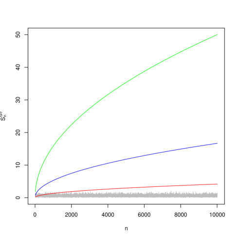
Figure 3: The statistics $\mathbf{S}_{n}^{(p)}$ $p=0,1,2,3$ as functions of the sample size. (“–”: $\mathbf{S}_{n}^{(0)}$ ), (“–”: $\mathbf{S}_{n}^{(1)}$), (“–”: $\mathbf{S}_{n}^{(2)}$), (“–”: $\mathbf{S}_{n}^{(3)}$).

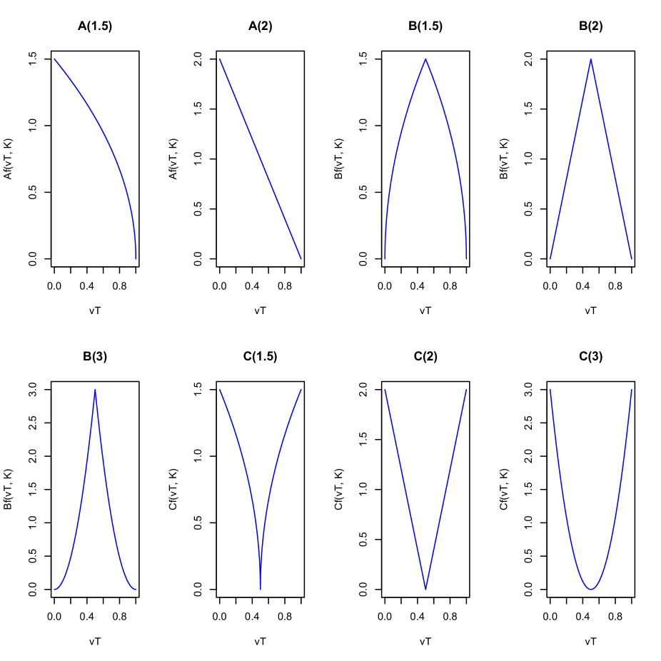
Figure 4: Densities of $A_{k}$, $B_{k}$, and $C_{k}$ families

$n=10$

1. Table 1: Powers (in percentages) of goodness of fit tests for the Uniform distribution on (0,1) for $n=10$ and $\alpha=0.01$

   $n$	Samples	Level
   10	10000	0.01

   Alternative	$\mathbf{S}_{n}^{(0)}$	$\mathbf{S}_{n}^{(1)}$	$\mathbf{S}_{n}^{(2)}$	$\mathbf{S}_{n}^{(3)}$
   $A_{1.5}$	4	7	7	0
   $A_{2}$	15	24	21	0
   $B_{1.5}$	0	1	1	0
   $B_{2}$	0	3	3	0
   $B_{3}$	0	7	9	0
   $C_{1.5}$	3	1	0	3
   $C_{2}$	6	1	1	8
   $C_{3}$	15	4	5	19

2. Table 2: Powers (in percentages) of goodness of fit tests for the Uniform distribution on (0,1) for $n=10$ and $\alpha=0.05$

   $n$	Samples	Level
   10	10000	0.05

   Alternative	$\mathbf{S}_{n}^{(0)}$	$\mathbf{S}_{n}^{(1)}$	$\mathbf{S}_{n}^{(2)}$	$\mathbf{S}_{n}^{(3)}$
   $A_{1.5}$	15	25	22	0
   $A_{2}$	38	54	48	0
   $B_{1.5}$	3	9	11	0
   $B_{2}$	4	17	20	0
   $B_{3}$	8	36	44	0
   $C_{1.5}$	11	5	5	13
   $C_{2}$	19	8	9	22
   $C_{3}$	36	18	21	38

3. Table 3: Powers (in percentages) of goodness of fit tests for the Uniform distribution on (0,1) for $n=10$ and $\alpha=0.10$

   $n$	Samples	Level
   10	10000	0.10

   Alternative	$\mathbf{S}_{n}^{(0)}$	$\mathbf{S}_{n}^{(1)}$	$\mathbf{S}_{n}^{(2)}$	$\mathbf{S}_{n}^{(3)}$
   $A_{1.5}$	25	37	32	0
   $A_{2}$	51	68	61	0
   $B_{1.5}$	8	18	19	3
   $B_{2}$	12	31	32	1
   $B_{3}$	24	58	61	0
   $C_{1.5}$	19	11	11	23
   $C_{2}$	30	16	16	32
   $C_{3}$	53	29	32	50

$n=20$

1. Table 4: Powers (in percentages) of goodness of fit tests for the Uniform distribution on (0,1) for $n=20$ and $\alpha=0.01$

   $n$	Samples	Level
   20	10000	0.01

   Alternative	$\mathbf{S}_{n}^{(0)}$	$\mathbf{S}_{n}^{(1)}$	$\mathbf{S}_{n}^{(2)}$	$\mathbf{S}_{n}^{(3)}$
   $A_{1.5}$	9	15	14	0
   $A_{2}$	39	52	49	0
   $B_{1.5}$	0	3	4	0
   $B_{2}$	1	8	13	0
   $B_{3}$	6	33	44	0
   $C_{1.5}$	4	1	1	6
   $C_{2}$	10	3	3	15
   $C_{3}$	31	14	16	40

2. Table 5: Powers (in percentages) of goodness of fit tests for the Uniform distribution on (0,1) for $n=20$ and $\alpha=0.05$

   $n$	Samples	Level
   20	10000	0.05

   Alternative	$\mathbf{S}_{n}^{(0)}$	$\mathbf{S}_{n}^{(1)}$	$\mathbf{S}_{n}^{(2)}$	$\mathbf{S}_{n}^{(3)}$
   $A_{1.5}$	28	42	37	0
   $A_{2}$	70	83	77	0
   $B_{1.5}$	6	15	16	0
   $B_{2}$	13	34	38	0
   $B_{3}$	42	74	78	0
   $C_{1.5}$	16	8	7	18
   $C_{2}$	31	17	17	36
   $C_{3}$	67	42	42	63

3. Table 6: Powers (in percentages) of goodness of fit tests for the Uniform distribution on (0,1) for $n=20$ and $\alpha=0.10$

   $n$	Samples	Level
   20	10000	0.10

   Alternative	$\mathbf{S}_{n}^{(0)}$	$\mathbf{S}_{n}^{(1)}$	$\mathbf{S}_{n}^{(2)}$	$\mathbf{S}_{n}^{(3)}$
   $A_{1.5}$	41	54	50	0
   $A_{2}$	81	89	86	0
   $B_{1.5}$	12	24	27	1
   $B_{2}$	27	48	53	0
   $B_{3}$	67	86	89	0
   $C_{1.5}$	25	14	14	30
   $C_{2}$	45	27	29	50
   $C_{3}$	82	55	56	75

$n=40$

1. Table 7: Powers (in percentages) of goodness of fit tests for the Uniform distribution on (0,1) for $n=40$ and $\alpha=0.01$

   $n$	Samples	Level
   40	10000	0.01

   Alternative	$\mathbf{S}_{n}^{(0)}$	$\mathbf{S}_{n}^{(1)}$	$\mathbf{S}_{n}^{(2)}$	$\mathbf{S}_{n}^{(3)}$
   $A_{1.5}$	25	37	35	0
   $A_{2}$	82	90	87	10
   $B_{1.5}$	1	7	10	0
   $B_{2}$	7	29	37	0
   $B_{3}$	49	83	89	6
   $C_{1.5}$	7	3	3	8
   $C_{2}$	24	13	13	27
   $C_{3}$	70	46	47	68

2. Table 8: Powers (in percentages) of goodness of fit tests for the Uniform distribution on (0,1) for $n=40$ and $\alpha=0.05$

   $n$	Samples	Level
   40	10000	0.05

   Alternative	$\mathbf{S}_{n}^{(0)}$	$\mathbf{S}_{n}^{(1)}$	$\mathbf{S}_{n}^{(2)}$	$\mathbf{S}_{n}^{(3)}$
   $A_{1.5}$	51	65	63	3
   $A_{2}$	95	98	97	28
   $B_{1.5}$	11	24	30	0
   $B_{2}$	38	62	70	3
   $B_{3}$	92	97	98	26
   $C_{1.5}$	24	13	14	27
   $C_{2}$	56	36	37	55
   $C_{3}$	96	77	75	87

3. Table 9: Powers (in percentages) of goodness of fit tests for the Uniform distribution on (0,1) for $n=40$ and $\alpha=0.10$

   $n$	Samples	Level
   40	10000	0.10

   Alternative	$\mathbf{S}_{n}^{(0)}$	$\mathbf{S}_{n}^{(1)}$	$\mathbf{S}_{n}^{(2)}$	$\mathbf{S}_{n}^{(3)}$
   $A_{1.5}$	65	77	74	5
   $A_{2}$	98	99	98	40
   $B_{1.5}$	23	37	42	1
   $B_{2}$	60	75	80	6
   $B_{3}$	98	99	99	43
   $C_{1.5}$	35	21	21	40
   $C_{2}$	74	50	49	69
   $C_{3}$	99	89	84	92

$n=100$

1. Table 10: Powers (in percentages) of goodness of fit tests for the Uniform distribution on (0,1) for $n=100$ and $\alpha=0.01$

   $n$	Samples	Level
   100	10000	0.01

   Alternative	$\mathbf{S}_{n}^{(0)}$	$\mathbf{S}_{n}^{(1)}$	$\mathbf{S}_{n}^{(2)}$	$\mathbf{S}_{n}^{(3)}$
   $A_{1.5}$	70	83	81	35
   $A_{2}$	99	100	100	97
   $B_{1.5}$	7	25	33	6
   $B_{2}$	56	83	89	52
   $B_{3}$	99	100	100	99
   $C_{1.5}$	17	13	12	24
   $C_{2}$	71	52	50	68
   $C_{3}$	99	97	95	98

2. Table 11: Powers (in percentages) of goodness of fit tests for the Uniform distribution on (0,1) for $n=100$ and $\alpha=0.05$

   $n$	Samples	Level
   100	10000	0.05

   Alternative	$\mathbf{S}_{n}^{(0)}$	$\mathbf{S}_{n}^{(1)}$	$\mathbf{S}_{n}^{(2)}$	$\mathbf{S}_{n}^{(3)}$
   $A_{1.5}$	91	96	94	58
   $A_{2}$	100	100	100	99
   $B_{1.5}$	34	54	61	17
   $B_{2}$	94	97	98	76
   $B_{3}$	100	100	100	99
   $C_{1.5}$	48	34	31	48
   $C_{2}$	96	81	75	86
   $C_{3}$	100	99	99	99

3. Table 12: Powers (in percentages) of goodness of fit tests for the Uniform distribution on (0,1) for $n=100$ and $\alpha=0.10$

   $n$	Samples	Level
   100	10000	0.10

   Alternative	$\mathbf{S}_{n}^{(0)}$	$\mathbf{S}_{n}^{(1)}$	$\mathbf{S}_{n}^{(2)}$	$\mathbf{S}_{n}^{(3)}$
   $A_{1.5}$	95	98	97	70
   $A_{2}$	100	100	100	99
   $B_{1.5}$	53	66	72	27
   $B_{2}$	98	98	99	86
   $B_{3}$	100	100	100	100
   $C_{1.5}$	66	46	44	62
   $C_{2}$	99	90	85	93
   $C_{3}$	100	100	99	99

We computed the power values of the proposed tests using Monte Carlo simulation and next these values are compared with each other. As it is expected, the power values of tests strongly depend on the type of alternatives. Based on our simulation study, against alternative $A_{k}$, the proposed tests $\mathbf{S}_{n}^{(1)}$ and $\mathbf{S}_{n}^{(2)}$ have a good power while against alternative $B_{k}$ the tests have the highest power compared with the classical Kolmogorov-Smirnov. The test based on $\mathbf{S}_{n}^{(3)}$ has a good power for alternative $C_{k}$. In order to extract methodological recommendations for the use of the proposed statistics in this work, it would be interesting to conduct extensive Monte Carlo experiments to compare our procedures with other alternatives presented in the literature, but this would go far beyond the scope of the present paper.

9 Mathematical developments

This section is devoted to the proofs of our results. The previously displayed notations continue to be used in the sequel.

9.1 Some bounds for the empirical process, Brownian bridge and the Kiefer process

Let us immediately point out an obvious fact which will be used several times thereafter:

$$0\leq F(t)\leq 1\quad\text{and}\quad 0\leq\mathbb{F}_{n}(t)\leq 1\quad\text{for}\quad t\in\mathbb{R},\,n\in\mathbb{N}^{*}$$

which obviously entails that, for any $p\in\mathbb{N}$,

$$0\leq F^{(p)}(t)\leq 1\quad\text{and}\quad 0\leq\mathbb{F}_{n}^{(p)}(t)\leq 1\quad\text{for}\quad t\in\mathbb{R},\,n\in\mathbb{N}^{*}.$$ (9.1)

Similarly, we have, for any $p\in\mathbb{N}$,

$$0\leq\mathbb{U}_{n}^{(p)}(u)\leq 1\quad\text{for}\quad u\in[0,1],\,n\in\mathbb{N}^{*}.$$ (9.2)

We also mention some bounds that we will use further. By appealing to Chung’s law of the iterated logarithm for the empirical process, see Chung (1949), which stipulates that

$$\limsup_{n\to\infty}\frac{\sup_{t\in\mathbb{R}}|\alpha_{n}(t)|}{\sqrt{\log\log n}}=\frac{1}{\sqrt{2}}\quad\text{a.s.},$$

we see that, with probability $1$, as $n\to\infty$,

$$\sup_{t\in\mathbb{R}}|\alpha_{n}(t)|=\mathcal{O}\!\left(\!\sqrt{\log\log n}\,\right)\!.$$ (9.3)

Moreover, by Komlós et al. (1975), on a suitable probability space, we can define the uniform empirical process $\{\beta_{n}:n\in\mathbb{N}^{*}\}$, in combination with a sequence of Brownian bridges $\left\{\mathbb{B}_{n}:n\in\mathbb{N}^{*}\right\}$ together with a Kiefer process $\{\mathbb{K}(s,u):s\geq 0,u\in[0,1]\}$, such that, with probability $1$, as $n\to\infty$,

$$\sup_{u\in[0,1]}\left|\beta_{n}(u)-\mathbb{B}_{n}(u)\right|=\mathcal{O}\!\left(\frac{\log n}{\sqrt{n}}\right)$$ (9.4)

and

$$\max_{1\leq k\leq n}\sup_{u\in[0,1]}\left|\sqrt{k}\,\beta_{k}(u)-\mathbb{K}(k,u)\right|=\mathcal{O}\!\left((\log n)^{2}\right)$$

from which we extract,with probability $1$, as $n\to\infty$,

$$\sup_{u\in[0,1]}\left|\beta_{n}(u)-\frac{1}{\sqrt{n}}\,\mathbb{K}(n,u)\right|=\mathcal{O}\!\left(\frac{(\log n)^{2}}{\sqrt{n}}\right)\!.$$ (9.5)

As a result, by putting (9.3) into (9.4) and (9.5), one derives the following bounds: with probability $1$, as $n\to\infty$,

$$\sup_{u\in[0,1]}|\mathbb{B}_{n}(u)|=\mathcal{O}\!\left(\!\sqrt{\log\log n}\,\right)\quad\text{and}\quad\sup_{u\in[0,1]}|\mathbb{K}(n,u)|=\mathcal{O}\!\left(\!\sqrt{n\log\log n}\,\right)\!.$$ (9.6)

Notice that the second bound in (9.6) comes also from the law of the iterated logarithm for the Kiefer process; see Csörgő and Révész (1981), p. 81.

9.2 Proof of Proposition 1.2

We begin by making an observation: because of the hypothesis that the df $F$ is continuous, the sampled variables $X_{1},X_{2},\ldots,X_{n}$ are almost surely all different. Then, we can define with probability $1$ the order statistics

$$X_{1,n}<X_{2,n}<\cdots<X_{n,n}$$

associated with $X_{1},X_{2},\ldots,X_{n}$. Notice that the event $\big{\{}X_{i,n}\leq t\big{\}}$ is equal to $\{n\mathbb{F}_{n}(t)\leq i\}$. Hence, we can write that, for any function $f$, with probability $1$,

$$\int_{-\infty}^{t}f(s)\,d\mathbb{F}_{n}(s)=\frac{1}{n}\sum_{i=1}^{n}f(X_{i})\mathbbm{1}_{\{X_{i}\leq t\}}=\frac{1}{n}\sum_{i=1}^{n\mathbb{F}_{n}(t)}f\!\left(X_{i,n}\right).$$ (9.7)

Before proving (1.6), we first show by induction that

$$\mathbb{F}_{n}^{(p)}(t)=\frac{1}{n^{p+1}}\#\left\{(i_{1},\dots,i_{p+1})\in\mathbb{N}^{p+1}:1\leq i_{1}\leq\dots\leq i_{p+1}\leq n\mathbb{F}_{n}(t)\right\}\!.$$ (9.8)

Of course, (9.8) holds for $p=0$. Pick now a positive integer $p$ and suppose that

$$\mathbb{F}_{n}^{(p-1)}(t)=\frac{1}{n^{p}}\#\left\{(i_{1},\dots,i_{p})\in\mathbb{N}^{p}:1\leq i_{1}\leq\dots\leq i_{p}\leq n\mathbb{F}_{n}(t)\right\}\!.$$

By Definition B.1, we see that the family of functions $\mathbb{F}_{n}^{(p)}$ can be recursively defined by $\mathbb{F}_{n}^{(0)}=\mathbb{F}_{n}$ and, for any $p\in\mathbb{N}^{*}$ and any $t\in\mathbb{R}$, by

$$\mathbb{F}_{n}^{(p)}(t)=\int_{-\infty}^{t}\mathbb{F}_{n}^{(p-1)}(s)\,d\mathbb{F}_{n}(s).$$

Therefore, by (9.7) and remarking that $\mathbb{F}_{n}(X_{i,n})=i/n$, a.s.,

$$\mathbb{F}_{n}^{(p)}(t) =\frac{1}{n}\sum_{i=1}^{n}\mathbb{F}_{n}^{(p-1)}(X_{i})\mathbbm{1}_{\{X_{i}\leq t\}}=\frac{1}{n}\sum_{i=1}^{n\mathbb{F}_{n}(t)}\mathbb{F}_{n}^{(p-1)}(X_{i,n})$$

$$=\frac{1}{n^{p+1}}\sum_{i=1}^{n\mathbb{F}_{n}(t)}\#\left\{(i_{1},\dots,i_{p})\in\mathbb{N}^{p}:1\leq i_{1}\leq\dots\leq i_{p}\leq n\mathbb{F}_{n}(X_{i,n})\right\}$$

$$=\frac{1}{n^{p+1}}\sum_{i=1}^{n\mathbb{F}_{n}(t)}\#\left\{(i_{1},\dots,i_{p})\in\mathbb{N}^{p}:1\leq i_{1}\leq\dots\leq i_{p}\leq i\right\}$$

$$=\frac{1}{n^{p+1}}\#\left\{(i_{1},\dots,i_{p},i_{p+1})\in\mathbb{N}^{p+1}:1\leq i_{1}\leq\dots\leq i_{p}\leq i_{p+1}\leq n\mathbb{F}_{n}(t)\right\}\!.$$

Hence, (9.8) is valid for any $p\in\mathbb{N}$.

Now, we observe that the cardinality in (9.8) is nothing but the number of combinations with repetitions of $p+1$ integers lying between $1$ and $n\mathbb{F}_{n}(t)$, which coincides with the number of combinations without repetition of $p+1$ integers lying between $1$ and $n\mathbb{F}_{n}(t)+p$. This is the result concerning $\mathbb{F}_{n}^{(p)}$ announced in (1.6). Finally, the formula concerning $F^{(p)}$ can be easily obtained by induction too. The proof of Proposition 1.2 is finished. $\Box$

In the proposition below, we provide a representation of $\mathbb{F}_{n}^{(p)}$ by means of $\mathbb{F}_{n}$.

Proposition 9.1

The integrated empirical d.f. $\mathbb{F}_{n}^{(p)}$ can be expressed by means of $\mathbb{F}_{n}$ as follows: with probability $1$,

$$\mathbb{F}_{n}^{(p)}(t)=\frac{\mathbb{F}_{n}(t)^{p+1}}{(p+1)!}+\sum_{k=1}^{p}a_{k}^{(p)}\,\frac{\mathbb{F}_{n}(t)^{k}}{n^{p-k+1}}\quad\text{for}\quad t\in\mathbb{R},\,n\in\mathbb{N}^{*},$$ (9.9)

where the coefficients $a_{k}^{(p)}$, $1\leq k\leq p$, are positive integers.

Proof. By expanding the combination in (1.6), we get that, a.s.,

$$\mathbb{F}_{n}^{(p)}(t)=\frac{1}{(p+1)!\,n^{p+1}}\,\prod_{i=0}^{p}(n\mathbb{F}_{n}(t)+i)=\frac{\mathbb{F}_{n}(t)}{(p+1)!\,n^{p}}\,\prod_{i=1}^{p}(n\mathbb{F}_{n}(t)+i)\quad\text{for}\quad t\in\mathbb{R},\,n\in\mathbb{N}^{*}.$$

Since $\prod_{i=1}^{p}(x+i)$ is a polynomial of degree $p$ with coefficients in $\mathbb{N}$, (9.9) immediately follows. $\Box$

In the proposition below, we rely $\alpha_{n}^{(p)}$ to $\alpha_{n}$.

Proposition 9.2

The $p$-fold integrated empirical process $\alpha_{n}^{(p)}$ is related to the empirical process $\alpha_{n}$ according to, with probability $1$,

$$\alpha_{n}^{(p)}(t)=\frac{1}{p!}\,F(t)^{p}\,\alpha_{n}(t)+\sum_{k=2}^{p+1}b_{k}^{(p)}\,\frac{F(t)^{p+1-k}}{n^{(k-1)/2}}\,\alpha_{n}(t)^{k}+\sum_{k=1}^{p}a_{k}^{(p)}\,\frac{\mathbb{F}_{n}(t)^{k}}{n^{p-k+1/2}}\quad\text{for}\quad t\in\mathbb{R},\,n\in\mathbb{N}^{*},$$ (9.10)

where the coefficients $a_{k}^{(p)}$, $1\leq k\leq p$, are those of Proposition 9.1 and the $b_{k}^{(p)}$, $2\leq k\leq p+1$, are positive real numbers less than $1$. Similarly,

$$\beta_{n}^{(p)}(u)=\frac{1}{p!}\,u^{p}\,\beta_{n}(u)+\sum_{k=2}^{p+1}b_{k}^{(p)}\,\frac{u^{p+1-k}}{n^{(k-1)/2}}\,\beta_{n}(u)^{k}+\sum_{k=1}^{p}a_{k}^{(p)}\,\frac{\mathbb{U}_{n}(u)^{k}}{n^{p-k+1/2}}\quad\text{for}\quad u\in[0,1],\,n\in\mathbb{N}^{*}.$$ (9.11)

Proof. By Definition B.1 and Formulae (1.6) and (9.9), we write that, a.s., for $t\in\mathbb{R},\,n\in\mathbb{N}^{*}$,

$$\alpha_{n}^{(p)}(t)=\frac{1}{(p+1)!}\,\sqrt{n}\left(\mathbb{F}_{n}(t)^{p+1}-F(t)^{p+1}\right)+\sum_{k=1}^{p}a_{k}^{(p)}\,\frac{\mathbb{F}_{n}(t)^{k}}{n^{p-k+1/2}}.$$

Applying the elementary identity below obtained by writing $a=(a-b)+b$ and using the binomial theorem

$$a^{p+1}-b^{p+1}=(p+1)b^{p}(a-b)+\sum_{k=2}^{p+1}{p+1\choose k}b^{p+1-k}(a-b)^{k}$$

to $a=\mathbb{F}_{n}(t)$ and $b=F(t)$ yields, a.s., for $t\in\mathbb{R},\,n\in\mathbb{N}^{*}$,

$$\alpha_{n}^{(p)}(t)= \;\frac{1}{p!}\,\sqrt{n}\,F(t)^{p}\left(\mathbb{F}_{n}(t)-F(t)\right)$$

$$+\frac{1}{(p+1)!}\,\sqrt{n}\,\sum_{k=2}^{p+1}{p+1\choose k}F(t)^{p+1-k}(\mathbb{F}_{n}(t)-F(t))^{k}$$

$$+\sum_{k=1}^{p}a_{k}^{(p)}\,\frac{\mathbb{F}_{n}(t)^{k}}{n^{p-k+1/2}}.$$ (9.12)

Substituting $\mathbb{F}_{n}(t)-F(t)=\alpha_{n}^{(p)}(t)/\sqrt{n}$ into (9.12) gives (9.10) by setting $b_{k}^{(p)}:={p+1\choose k}/(p+1)!$. $\Box$

9.3 Proof of Theorem 2.2

Set $A_{p}:=\sum_{k=1}^{p}a_{k}^{(p)}>0$ and $I=[0,d/n]$ or $[1-d/n,1]$. Making use of (9.11) together with (9.2) and the fact that $0\leq b_{k}^{(p)}\leq 1$, it is clear that, a.s., for any $d,n\in\mathbb{N}^{*}$ such that $d\leq n$,

$$\sup_{u\in I}\left|\beta_{n}^{(p)}(u)-\mathbb{B}_{n}^{(p)}(u)\right|\leq\sup_{u\in I}\big{|}\beta_{n}(u)-\mathbb{B}_{n}(u)\big{|}+\frac{1}{\sqrt{n}}\sum_{k=2}^{p+1}\frac{1}{n^{k/2-1}}\sup_{u\in[0,1]}|\beta_{n}(u)|^{k}+\frac{A_{p}}{\sqrt{n}}.$$

Therefore,

$$\leq\mathbb{P}\bigg{\{}\sup_{u\in I}|\beta_{n}(u)-\mathbb{B}_{n}(u)|+\frac{1}{\sqrt{n}}\,\sum_{k=2}^{p+1}\frac{1}{n^{k/2-1}}\,\sup_{u\in[0,1]}|\beta_{n}(u)|^{k}\geq\frac{1}{\sqrt{n}}\,(c_{1}\log d+x-A_{p})\bigg{\}}\!.$$

Now, using the elementary inequality

$$\mathbb{P}\!\left\{\sum_{k=1}^{r}\xi_{k}\geq\sum_{k=1}^{r}a_{k}\right\}\leq\sum_{k=1}^{r}\mathbb{P}\{\xi_{k}\geq a_{k}\},$$

which is valid for any positive integer $r$, any r.v.’s $\xi_{1},\dots,\xi_{r}$ and any real numbers $a_{1},\dots,a_{r}$, we obtain

$$\leq \;\mathbb{P}\bigg{\{}\sup_{u\in I}|\beta_{n}(u)-\mathbb{B}_{n}(u)|\geq\frac{1}{\sqrt{n}}\,(c_{1}\log d+\frac{x}{p+1}-A_{p})\bigg{\}}$$

$$+\sum_{k=2}^{p+1}\mathbb{P}\bigg{\{}\sup_{u\in[0,1]}|\beta_{n}(u)|^{k}\geq\frac{xn^{k/2-1}}{p+1}\bigg{\}}\!.$$ (9.13)

On the other hand, the inequality of Dvoretzky et al. (1956) stipulates that there exists a positive constant $c_{4}$ such that, for any $x>0$ and any $n\in\mathbb{N}^{*}$,

$$\mathbb{P}\left\{\sup_{t\in\mathbb{R}}\left|\mathbb{F}_{n}(t)-F(t)\right|\geq\frac{x}{\sqrt{n}}\,\right\}\leq c_{4}\,\exp({-2x^{2}}).$$ (9.14)

Actually (9.14) simply reads, by means of $\beta_{n}$, for any $x>0$ and any $n\in\mathbb{N}^{*}$, as

$$\mathbb{P}\bigg{\{}\sup_{u\in[0,1]}|\beta_{n}(u)|\geq x\bigg{\}}\leq c_{4}\,\exp({-2x^{2}}).$$

Then,

$$\sum_{k=2}^{p+1}\mathbb{P}\bigg{\{}\sup_{u\in[0,1]}|\beta_{n}(u)|^{k}\geq\frac{xn^{k/2-1}}{p+1}\bigg{\}} \leq c_{4}\sum_{k=2}^{p+1}\exp\!\left(-2\left(\frac{x{\,n^{k/2-1}}}{p+1}\right)^{\!\!2/k}\right)$$

$$\leq c_{4}\!\left(\exp({-[2/(p+1)]\,x})+\sum_{k=3}^{p+1}\exp\!\left(-\frac{2}{p+1}\,x^{2/k}n^{1-2/k}\right)\!\right)\!.$$ (9.15)

Now, by putting (2.1) and (9.15) into (9.13), we immediately complete the proof of Theorem 2.2 with

$$B_{p}:=c_{2}\,\exp({c_{3}A_{p}})+c_{4}\quad\text{and}\quad C_{p}:=\min(c_{3},2)/(p+1).$$

$\Box$

9.4 Proof of Corollary 2.4

The functional $\Phi$ being Lipschitz, there exists a positive constant $L$ such that, for any functions $v,w$,

$$|\Phi(v)-\Phi(w)|\leq L\sup_{t\in\mathbb{R}}|v(t)-w(t)|.$$ (9.16)

Let us choose for $v,w$ the processes

$$V_{n}:=\alpha_{n}^{(p)}(\cdot)\quad\mbox{and}\quad W_{n}:=\mathbb{B}_{n}^{(p)}(F(\cdot)).$$

Applying the elementary inequality

$$|\mathbb{P}(A)-\mathbb{P}(B)|\leq\mathbb{P}(A\backslash B)+\mathbb{P}(B\backslash A)=\mathbb{P}\big{(}(A\backslash B)\cup(B\backslash A)\big{)}$$

to the events $A=\{\Phi(V_{n})\leq x\}$ and $B=\{\Phi(W_{n})\leq x\}$ provides, for any $x\in\mathbb{R}$ and any $n\in\mathbb{N}^{*}$,

$$\big{|}\mathbb{P}\{\Phi(V_{n})\leq x\}-\mathbb{P}\{\Phi(W_{n})\leq x\}\big{|}\leq\mathbb{P}\{\Phi(V_{n})\leq x\leq\Phi(W_{n})\quad\mbox{or}\quad\Phi(W_{n})\leq x\leq\Phi(V_{n})\}.$$

Now, applying to the elementary fact that [$a\leq x\leq b$ or $b\leq x\leq a$ implies $|b-x|\leq|b-a|$] to the numbers $a=\Phi(V_{n})$ and $b=\Phi(W_{n})$

$$\mathbb{P}\{\Phi(V_{n})\leq x\leq\Phi(W_{n})\;\mbox{or}\;\Phi(W_{n})\leq x\leq\Phi(V_{n})\} \leq\mathbb{P}\!\left\{|\Phi(W_{n})-x|\leq|\Phi(W_{n})-\Phi(V_{n})|\right\}\!,$$

from which, due to (9.16), we deduce that

$$\big{|}\mathbb{P}\{\Phi(V_{n})\leq x\}-\mathbb{P}\{\Phi(W_{n})\leq x\}\big{|}\leq\mathbb{P}\!\left\{|\Phi(W_{n})-x|\leq L\sup_{t\in\mathbb{R}}|V_{n}(t)-W_{n}(t)|\right\}\!.$$ (9.17)

On the other hand, by choosing $x=c\log n$ for a large enough constant $c$ in (2.4) and putting $\epsilon_{n}:=(c+c_{1})$ $\log n/\sqrt{n}$, we obtain the estimate below valid for large enough $n$:

$$\mathbb{P}\!\left\{\sup_{t\in\mathbb{R}}\left|V_{n}(t)-W_{n}(t)\right|\geq\epsilon_{n}\right\}\leq\frac{B_{p}}{n}=o\!\left(\frac{\log n}{\sqrt{n}}\right)\!.$$ (9.18)

Now, by (9.17), we write

$$\leq \;\mathbb{P}\!\left\{\sup_{t\in\mathbb{R}}\left|V_{n}(t)-W_{n}(t)\right|<\epsilon_{n},|\Phi(W_{n})-x|\leq L\sup_{t\in\mathbb{R}}|V_{n}(t)-W_{n}(t)|\right\}$$

$$+\mathbb{P}\!\left\{\sup_{t\in\mathbb{R}}\left|V_{n}(t)-W_{n}(t)\right|\geq\epsilon_{n},|\Phi(W_{n})-x|\leq L\sup_{t\in\mathbb{R}}|V_{n}(t)-W_{n}(t)|\right\}$$

$$\leq \;\mathbb{P}\!\left\{|\Phi(W_{n})-x|\leq L\epsilon_{n}\right\}+\mathbb{P}\!\left\{\sup_{t\in\mathbb{R}}\left|V_{n}(t)-W_{n}(t)\right|\geq\epsilon_{n}\right\}\!.$$ (9.19)

Noticing that the distribution of $\mathbb{B}_{n}$ does not depend on $n$, which entails the equality

$$\mathbb{P}\!\left\{|\Phi(W_{n})-x|\leq L\epsilon_{n}\right\}=\mathbb{P}\!\left\{|\Phi(W)-x|\leq L\epsilon_{n}\right\}$$

where

$$W:=F(\cdot)^{p}\,\mathbb{B}(F(\cdot))/p!,$$

and recalling the assumption that the r.v. $\Phi(W)$ admits a density function bounded by $M$ say, we get that, for any $x\in\mathbb{R}$ and any $n\in\mathbb{N}^{*}$,

$$\mathbb{P}\!\left\{|\Phi(W_{n})-x|\leq L\epsilon_{n}\right\}\leq 2LM\epsilon_{n}.$$ (9.20)

Finally, putting (9.18) and (9.20) into (9.19) leads to (2.5), which completes the proof of Corollary 2.4. An alternative proof of a similar result may be found in Shorack and Wellner (1986) pp. 502–503. $\Box$

9.5 Proof of Corollary 2.5

Set, for any $n\in\mathbb{N}^{*}$,

$$\pi_{n}:=\mathbb{P}\!\left\{\sup_{t\in\mathbb{R}}\left|\alpha_{n}^{(p)}(t)-\mathbb{B}_{n}^{(p)}(F(t))\right|\geq c_{6}\,\frac{\log n}{\sqrt{n}}\right\}\!.$$

Applying (2.4) to $x=c^{\prime}\log n$ for a sufficiently large constant $c^{\prime}$ yields, for large enough $n$,

$$\pi_{n} \leq B_{p}\sum_{k=2}^{p+1}\exp\!\left(-C_{p}c^{\prime 2/k}\,(\log n)^{2/k}n^{1-3/k}\right)$$

$$=\mathcal{O}\!\left(\frac{1}{n^{2}}\right),$$

where $c_{6}$ is a positive constant. Hence the series $(\sum_{n\geq 1}\pi_{n})$ is convergent and by appealing to Borel-Cantelli lemma, we get that

$$\mathbb{P}\!\left(\limsup_{n\in\mathbb{N}^{*}}\left\{\sup_{t\in\mathbb{R}}\left|\alpha_{n}^{(p)}(t)-\mathbb{B}_{n}^{(p)}(F(t))\right|\geq c_{6}\,\frac{\log n}{\sqrt{n}}\right\}\right)=0,$$

which clearly implies Corollary 2.5. $\Box$

9.6 Proof of Theorem 2.6

In view of (9.10), we write that, a.s., for any $s\in(0,1)$, any $t\in\mathbb{R}$ and any $k\in\mathbb{N}^{*}$,

$$\sqrt{k}\,\alpha_{k}^{(p)}(t)-\mathbb{K}^{(p)}(k,F(t))= \;\frac{1}{p!}\,F(t)^{p}\left[\sqrt{k}\,\alpha_{k}(t)-\mathbb{K}(k,F(t))\right]$$

$$+\sum_{i=2}^{p+1}b_{i}^{(p)}\,\frac{F(t)^{p+1-i}}{k^{(i-1)/2}}\,\alpha_{k}(t)^{i}+\sum_{i=1}^{p}a_{i}^{(p)}\,\frac{\mathbb{F}_{k}(t)^{i}}{k^{p-i+1/2}}.$$ (9.21)

Then, by using (9.1) together with the fact that $0\leq b_{i}^{(p)}\leq 1$, we deduce that, a.s., for any $n\in\mathbb{N}^{*}$,

$$\leq\frac{1}{p!}\,\max_{1\leq k\leq n}\sup_{t\in\mathbb{R}}\left|\sqrt{k}\,\alpha_{k}(t)-\mathbb{K}(k,F(t))\right|+\sum_{i=2}^{p+1}\max_{1\leq k\leq n}\!\left(\frac{1}{k^{(i-1)/2}}\sup_{t\in\mathbb{R}}|\alpha_{k}(t)|^{i}\right)$$

$$+\sum_{i=1}^{p}\max_{1\leq k\leq n}\frac{a_{i}^{(p)}}{k^{p-i+1/2}}$$

$$\leq\max_{1\leq k\leq n}\sup_{t\in\mathbb{R}}\left|\sqrt{k}\,\alpha_{k}(t)-\mathbb{K}(k,F(t))\right|+\sum_{i=2}^{p+1}\left(\max_{1\leq k\leq n}\sup_{t\in\mathbb{R}}|\alpha_{k}(t)|\right)^{\!i}+A_{p}.$$ (9.22)

Finally, by putting (9.5) and (9.3) into (9.22), we completes the proof of Theorem 2.6. $\Box$

9.7 Proof of Corollary 2.7

From Theorem 2.6, we deduce that, with probability $1$, as $n\to\infty$,

$$\sup_{t\in\mathbb{R}}\big{|}\alpha_{n}^{(p)}(t)\big{|}=\frac{1}{\sqrt{n}}\,\sup_{t\in\mathbb{R}}\big{|}\mathbb{K}^{(p)}(n,F(t))\big{|}+\mathcal{O}\!\left(\frac{(\log n)^{2}}{\sqrt{n}}\right)\!.$$

Therefore, a.s.,

$$\limsup_{n\to\infty}\frac{\sup_{t\in\mathbb{R}}\big{|}\alpha_{n}^{(p)}(t)\big{|}}{\sqrt{\log\log n}} =\limsup_{n\to\infty}\frac{\sup_{t\in\mathbb{R}}\big{|}\mathbb{K}^{(p)}(n,F(t))\big{|}}{\sqrt{n\log\log n}}$$

$$=\limsup_{n\to\infty}\frac{\sup_{u\in[0,1]}|u^{p}\,\mathbb{K}(n,u)|}{p!\,\sqrt{n\log\log n}}$$

$$=\frac{\sqrt{2}}{p!}\sup_{u\in[0,1]}\sqrt{\mathrm{Var}(u^{p}\,\mathbb{K}(1,u))}.$$ (9.23)

In the last equality, we have used Strassen’s law of the iterated logarithm for Gaussian processes; see for instance Oodaira (1973), or Corollary 1.15.1 of Csörgő and Révész (1981). Observing that $\mathrm{Var}(u^{p}\,\mathbb{K}(1,u))=u^{2p+1}(1-u)$ and that

$$\sup_{u\in[0,1]}u^{2p+1}(1-u)=\frac{(2p+1)^{2p+1}}{(2p+2)^{2p+2}},$$

(9.23) readily implies (2.7) which proves Corollary 2.7. $\Box$

9.8 Proof of Corollary 2.8

We work under Hypothesis $\mathcal{H}_{0}$. Let us introduce the $p$-fold integrated empirical process related to the d.f. $F_{0}$:

$$\alpha_{0,n}^{(p)}(t):=\sqrt{n}\left(\mathbb{F}_{n}^{(p)}(t)-F_{0}^{(p)}(t)\right)\quad\text{for}\quad t\in\mathbb{R},\,n\in\mathbb{N}^{*}.$$

By the triangular inequality, we plainly have

$$\left|\mathbf{S}_{n}^{(p)}-\sup_{t\in\mathbb{R}}\big{|}\mathbb{B}_{n}^{(p)}(F_{0}(t))\big{|}\right|\leq\sup_{t\in\mathbb{R}}\left|\alpha_{0,n}^{(p)}(t)-\mathbb{B}_{n}^{(p)}(F_{0}(t))\right|$$

from which together with (2.6) we deduce (2.8).

Similarly,

$$\left|\mathbf{T}_{n}^{(p)}-\int_{\mathbb{R}}\big{[}\mathbb{B}_{n}^{(p)}(F_{0}(t))\big{]}^{2}\,dF_{0}(t)\right|\leq \;\int_{\mathbb{R}}\left|\alpha_{0,n}^{(p)}(t)^{2}-\big{[}\mathbb{B}_{n}^{(p)}(F_{0}(t))\big{]}^{2}\right|dF_{0}(t)$$

$$\leq \;\sup_{t\in\mathbb{R}}\left|\alpha_{0,n}^{(p)}(t)-\mathbb{B}_{n}^{(p)}(F_{0}(t))\right|$$

$$\times\left(\sup_{t\in\mathbb{R}}\left|\alpha_{0,n}^{(p)}(t)\right|+\sup_{t\in\mathbb{R}}\big{|}\mathbb{B}_{n}^{(p)}(F_{0}(t))\big{|}\right)\!.$$ (9.24)

In the last inequality above appears the supremum

$$\sup_{t\in\mathbb{R}}\big{|}\mathbb{B}_{n}^{(p)}(F_{0}(t))\big{|}\leq\sup_{u\in[0,1]}\big{|}\mathbb{B}_{n}(u)\big{|}.$$

Then, by putting (2.6), (2.7) and (9.6) into (9.24), we immediately deduce (2.9). The proof of Corollary 2.8 is finished. $\Box$

9.9 Proof of Theorem 3.1

We imitate the proof of Theorem 2.1 in Mason (2001). Let us introduce

$$\Delta_{n,\nu}^{(p)}(d) :=\sup_{u\in[d/n,1-d/n]}\frac{\big{|}\beta_{n}^{(p)}(u)-\mathbb{B}_{n}^{(p)}(u)\big{|}}{\big{(}u(1-u)\big{)}^{\nu}},$$

$$\Delta_{n,\nu}^{1,(p)}(d) :=\sup_{u\in[d/n,1]}\frac{\big{|}\beta_{n}^{(p)}(u)-\mathbb{B}_{n}^{(p)}(u)\big{|}}{u^{\nu}},$$

$$\Delta_{n,\nu}^{2,(p)}(d) :=\sup_{u\in[0,1-d/n]}\frac{\big{|}\beta_{n}^{(p)}(u)-\mathbb{B}_{n}^{(p)}(u)\big{|}}{(1-u)^{\nu}}.$$

We clearly have

$$\Delta_{n,\nu}^{1,(p)}(d) =\max\!\left(\sup_{u\in[d/n,1/2]}\frac{\big{|}\beta_{n}^{(p)}(u)-\mathbb{B}_{n}^{(p)}(u)\big{|}}{\big{(}u(1-u)\big{)}^{\nu}},\sup_{u\in[1/2,1-d/n]}\frac{\big{|}\beta_{n}^{(p)}(u)-\mathbb{B}_{n}^{(p)}(u)\big{|}}{\big{(}u(1-u)\big{)}^{\nu}}\right)$$

$$\leq 2^{\nu}\max\!\left(\sup_{u\in[d/n,1/2]}\frac{\big{|}\beta_{n}^{(p)}(u)-\mathbb{B}_{n}^{(p)}(u)\big{|}}{u^{\nu}},\sup_{u\in[1/2,1-d/n]}\frac{\big{|}\beta_{n}^{(p)}(u)-\mathbb{B}_{n}^{(p)}(u)\big{|}}{(1-u)^{\nu}}\right)$$

which entails that

$$\Delta_{n,\nu}^{(p)}(d)\leq 2^{\nu}\max\!\left(\Delta_{n,\nu}^{1,(p)}(d),\Delta_{n,\nu}^{2,(p)}(d)\right)\!.$$ (9.25)

Hence, it suffices to derive inequalities of the form (3.1) for the auxiliary quantities $\Delta_{n,\nu}^{(p)1}(d)$ and $\Delta_{n,\nu}^{(p)2}(d)$. First, notice that if we have for each $i\in\{d,\dots,n-1\}$,

$$\sup_{u\in[0,(i+1)/n]}\big{|}\beta_{n}^{(p)}(u)-\mathbb{B}_{n}^{(p)}(u)\big{|}<x(i/n)^{\nu},$$

then

$$\Delta_{n,\nu}^{1,(p)}(d) =\max_{i=d,\dots,n-1}\!\left(\sup_{u\in[i/n,(i+1)/n]}\frac{\big{|}\beta_{n}^{(p)}(u)-\mathbb{B}_{n}^{(p)}(u)\big{|}}{u^{\nu}}\right)$$

$$\leq\max_{i=d,\dots,n-1}\!\bigg{(}\!\!\left(\frac{n}{i}\right)^{\nu}\sup_{u\in[0,(i+1)/n]}\big{|}\beta_{n}^{(p)}(u)-\mathbb{B}_{n}^{(p)}(u)\big{|}\bigg{)}<x.$$

Hence, we derive the inequality

$$\mathbb{P}\big{\{}\Delta_{n,\nu}^{1,(p)}(d)\geq x\big{\}}\leq\sum_{i=d}^{n-1}\delta_{i,n},$$ (9.26)

where

$$\delta_{i,n}:=\mathbb{P}\bigg{\{}\sup_{u\in[0,(i+1)/n]}\big{|}\beta_{n}^{(p)}(u)-\mathbb{B}_{n}^{(p)}(u)\big{|}\geq x(i/n)^{\nu}\bigg{\}}.$$

Quite similarly,

$$\mathbb{P}\big{\{}\Delta_{n,\nu}^{2,(p)}(d)\geq x\big{\}}\leq\sum_{i=0}^{n-d-1}\delta_{i,n}.$$ (9.27)

Set now (under the assumption $\nu>0$)

$$a_{\nu}:=\max\!\left(\!1,c_{1}\sup_{i\in\mathbb{N}^{*}}\frac{\log(i+1)}{i^{\nu}}\right),$$

where the constant $c_{1}$ is that of (2.1). Of course, $a_{\nu}\geq 1$ and, for any $i\in\mathbb{N}^{*}$,

$$a_{\nu}\,i^{\nu}\geq c_{1}\log(i+1).$$

Then, by writing

$$x=(x-a_{\nu}n^{\nu-1/2})+a_{\nu}n^{\nu-1/2}$$

in $\delta_{i,n}$ above and appealing to (2.3), we have, for $i\geq d$, any $n\in\mathbb{N}^{*}$ and large enough $x$ (recall the assumption $\nu<1/2$),

$$\delta_{i,n} \leq\mathbb{P}\bigg{\{}\sup_{u\in[0,(i+1)/n]}\big{|}\beta_{n}^{(p)}(u)-\mathbb{B}_{n}^{(p)}(u)\big{|}\geq\frac{1}{\sqrt{n}}\left(c_{1}\log(i+1)+i^{\nu}(xn^{1/2-\nu}-a_{\nu})\right)\!\bigg{\}}$$

$$\leq B_{p}\sum_{k=2}^{p+1}\exp\!\left(-C_{p}\,(xn^{1/2-\nu}-a_{\nu})^{2/k}i^{2\nu/k}n^{1-2/k}\right)\!.$$ (9.28)

In order to split the quantity $(xn^{1/2-\nu}-a_{\nu})^{2/k}$, we use the elementary inequality

$$(a+b)^{\mu}\geq 2^{\mu-1}\big{(}a^{\mu}+b^{\mu}\big{)},$$

which is valid for any $a,b\geq 0$ and any $\mu\in(0,1]$. If, in addition, $a$ and $b$ satisfy $a\geq 4b$, which entails that

$$a-2b\geq a/2,$$

then

$$(a-b)^{\mu}\geq 2^{\mu-1}\big{(}(a-2b)^{\mu}+b^{\mu}\big{)}\geq\frac{1}{2}\big{(}a^{\mu}+b^{\mu}\big{)}.$$

Thanks to this last inequality, we can write, for any $i\geq d$, any $k\leq p+1$ and any $x\geq 4a_{\nu}n^{\nu-1/2}$, that

$$\leq\exp\!\left(-C_{p}^{\prime\prime}\,a_{\nu}^{2/k}i^{2\nu/k}n^{1-2/k}\right)\exp\!\left(-C_{p}^{\prime\prime}\,x^{2/k}d^{2\nu/k}n^{1-(2\nu+1)/k}\right)$$

$$\leq\exp\!\left(-C_{p}^{\prime\prime}\,i^{2\nu/(p+1)}\right)\exp\!\left(-C_{p}^{\prime\prime}\,x^{2/k}d^{2\nu/k}n^{1-(2\nu+1)/k}\right),$$ (9.29)

where we set $C_{p}^{\prime\prime}=C_{p}/2$. Consequently, by putting (9.29) into (9.28), and next this latter into (9.26) and (9.27), we get

$$\mathbb{P}\big{\{}\Delta_{n,\nu}^{1,(p)}(d)\geq x\big{\}}\quad\text{and}\quad\mathbb{P}\big{\{}\Delta_{n,\nu}^{2,(p)}(d)\geq x\big{\}}\leq\frac{1}{2}\,B_{p,\nu}\sum_{k=2}^{p+1}\exp\!\left(-C_{p}^{\prime\prime}\,x^{2/k}d^{2\nu/k}n^{1-(2\nu+1)/k}\right)\!,$$ (9.30)

with the constant

$$B_{p,\nu}:=2B_{p}\sum_{i=0}^{\infty}\exp\!\left(-C_{p}^{\prime\prime}i^{2\nu/(p+1)}\right)<+\infty.$$

Finally, by (9.25),

$$\mathbb{P}\big{\{}\Delta_{n,\nu}^{(p)}(d)\geq x\big{\}}\leq\mathbb{P}\!\left\{\Delta_{n,\nu}^{1,(p)}(d)\geq\frac{x}{2}\right\}+\mathbb{P}\!\left\{\Delta_{n,\nu}^{2,(p)}(d)\geq\frac{x}{2}\right\},$$ (9.31)

and by putting (9.30) into (9.31), we obtain (3.1) with $C_{p}^{\prime}=C_{p}^{\prime\prime}/2^{2/(p+1)}$. $\Box$

9.10 Proof of Corollary 3.2

Applying (3.1) to $x=c^{\prime\prime}\log n$ for a sufficiently large constant $c^{\prime\prime}$ yields, for large enough $n$,

$$\mathbb{P}\bigg{\{}\Delta_{n,\nu}^{(p)}(d)\geq c^{\prime\prime}\frac{\log n}{n^{1/2-\nu}}\bigg{\}}\leq \;B_{p,\nu}\sum_{k=2}^{p+1}\exp\!\left(-C_{p}^{\prime}c^{\prime\prime 2/k}\,d^{2\nu/k}(\log n)^{2/k}n^{1-2/k}\right)$$

$$= \;\mathcal{O}\!\left(\frac{1}{n^{2}}\right)\!.$$

We conclude with the aid of Borel-Cantelli lemma as in Subsection 9.5. $\Box$

9.11 Proof of Corollary 4.1

For each $m,n\in\mathbb{N}^{*}$, let $\alpha_{m}^{1,(p)}$ and $\alpha_{n}^{2,(p)}$ denote the empirical processes respectively associated with the samples $X_{1},\ldots,X_{m}$ and $Y_{1},\ldots,Y_{n}$. By replacing $\mathbb{F}_{m}^{(p)}(t)$ by $\alpha_{m}^{1,(p)}(t)/\sqrt{m}+F^{(p)}(t)$ and $\mathbb{G}_{n}^{(p)}(t)$ by $\alpha_{n}^{2,(p)}(t)/\sqrt{n}+G^{(p)}(t)$, using the binomial theorem and recalling that, under $\mathcal{H}_{0}^{\prime}$, $F=G$, we write

$$\boldsymbol{\xi}_{m,n}^{(p,q)}(t) =\sqrt{\frac{mn}{m+n}}\left[\left(\frac{\alpha_{m}^{1,(p)}(t)}{\sqrt{m}}+F^{(p)}(t)\right)^{\!\!q}-\left(\frac{\alpha_{n}^{2,(p)}(t)}{\sqrt{n}}+F^{(p)}(t)\right)^{\!\!q}\right]$$

$$=\sqrt{\frac{mn}{m+n}}\sum_{k=1}^{q}{q\choose k}\big{(}F^{(p)}(t)\big{)}^{q-k}\left[\left(\frac{\alpha_{m}^{1,(p)}(t)}{\sqrt{m}}\right)^{\!\!k}-\left(\frac{\alpha_{n}^{2,(p)}(t)}{\sqrt{n}}\right)^{\!\!k}\right]$$

$$=q\big{(}F^{(p)}(t)\big{)}^{q-1}\left(\sqrt{\frac{n}{m+n}}\,\alpha_{m}^{1,(p)}(t)-\sqrt{\frac{m}{m+n}}\,\alpha_{n}^{2,(p)}(t)\right)+\Delta_{m,n}(t)$$

where

$$\Delta_{m,n}(t)=\sqrt{\frac{mn}{m+n}}\sum_{k=2}^{q}{q\choose k}\big{(}F^{(p)}(t)\big{)}^{q-k}\left[\left(\frac{\alpha_{m}^{1,(p)}(t)}{\sqrt{m}}\right)^{\!\!k}-\left(\frac{\alpha_{n}^{2,(p)}(t)}{\sqrt{n}}\right)^{\!\!k}\right]\!.$$

By (2.7) and (9.1), it is easily seen that, with probability $1$, as $m,n\to\infty$,

$$\sup_{t\in\mathbb{R}}|\Delta_{m,n}(t)|=\mathcal{O}\!\left(\frac{(\log\log m)^{q/2}}{\sqrt{m}}\right)+\mathcal{O}\!\left(\frac{(\log\log n)^{q/2}}{\sqrt{n}}\right)\!.$$ (9.32)

On the other hand, by Corollary 2.5, we can construct two sequences of Brownian bridges $\big{\{}\mathbb{B}_{m}^{1}:m\in\mathbb{N}^{*}\big{\}}$ and $\big{\{}\mathbb{B}_{n}^{2}:n\in\mathbb{N}^{*}\big{\}}$ such that, with probability $1$, as $m,n\to\infty$,

$$\sup_{t\in\mathbb{R}}\left|\alpha_{m}^{1,(p)}(t)-\frac{1}{p!}\,F(t)^{p}\,\mathbb{B}_{m}^{1}(F(t))\right| =\mathcal{O}\!\left(\frac{\log m}{\sqrt{m}}\right)\!,$$

$$\sup_{t\in\mathbb{R}}\left|\alpha_{n}^{2,(p)}(t)-\frac{1}{p!}\,F(t)^{p}\,\mathbb{B}_{n}^{2}(F(t))\right| =\mathcal{O}\!\left(\frac{\log n}{\sqrt{n}}\right)\!.$$

Setting $\mathbb{B}_{m,n}^{(p,q)}$ as in Corollary 4.1, we have

$$\boldsymbol{\xi}_{m,n}^{(p,q)}(t)-\mathbb{B}_{m,n}^{(p,q)}(t)= \;\frac{q}{(p+1)!^{q-1}}\,F(t)^{(p+1)(q-1)}\left[\sqrt{\frac{n}{m+n}}\left(\alpha_{m}^{1,(p)}(t)-\frac{1}{p!}\,F(t)^{p}\,\mathbb{B}_{m}^{1}(F(t))\right)\right.$$

$$\left.-\sqrt{\frac{m}{m+n}}\left(\alpha_{n}^{2,(p)}(t)-\frac{1}{p!}\,F(t)^{p}\,\mathbb{B}_{n}^{2}(F(t))\right)\right]+\Delta_{m,n}(t).$$ (9.34)

By putting (9.32) and (LABEL:ecart1) into (9.34), we deduce the result announced in Corollary 4.1. $\Box$

9.12 Proof of Theorem 4.4

Let us introduce, for each $k\in\{1,\dots,K\}$, the $p$-fold integrated empirical process associated with the d.f. $F^{k}$

$$\alpha_{n}^{k,(p)}(t):=\sqrt{n}\left(\mathbb{F}_{n}^{k,(p)}(t)-F^{k,(p)}(t)\right)\quad\text{for}\quad t\in\mathbb{R},\,n\in\mathbb{N}^{*}.$$

By recalling (4.1) and making use of the most well-known variance formula

$$\sum_{k=1}^{K}n_{k}(x_{k}-\bar{x})^{2}=\sum_{k=1}^{K}n_{k}(x_{k}-x_{0})^{2}-\boldsymbol{|n|}\left(\bar{x}-x_{0}\right)^{2},$$

where we have denoted

$$\boldsymbol{|n|}=\sum_{k=1}^{K}n_{k}~{}~{}\mbox{and}~{}~{}\bar{x}=\frac{1}{\boldsymbol{|n|}}\sum_{k=1}^{K}n_{k}x_{k},~{}~{}\mbox{ for}~{}~{}\boldsymbol{n}=(n_{1},\dots,n_{K}),$$

we rewrite $\boldsymbol{\xi}_{K,\boldsymbol{n}}^{(p)}(t)$ under Hypothesis $\mathcal{H}_{0}^{K}$ as

$$\boldsymbol{\xi}_{K,\boldsymbol{n}}^{(p)}(t) =\sum_{k=1}^{K}n_{k}\!\left(\mathbb{F}_{n_{k}}^{k,(p)}(t)-F_{0}^{(p)}(t)\right)^{\!2}-\frac{1}{\boldsymbol{|n|}}\left(\sum_{k=1}^{K}n_{k}\!\left(\mathbb{F}_{n_{k}}^{k,(p)}(t)-F_{0}^{(p)}(t)\right)\right)^{\!\!2}$$

$$=\sum_{k=1}^{K}\alpha_{n_{k}}^{k,(p)}(t)^{2}-\left(\sum_{k=1}^{K}\sqrt{\frac{n_{k}}{\boldsymbol{|n|}}}\,\alpha_{n_{k}}^{k,(p)}(t)\right)^{\!\!2}.$$

Next, setting $\mathbb{B}_{K,\boldsymbol{n}}^{(p)}$ as in Theorem 4.4, we have

$$\boldsymbol{\xi}_{K,\boldsymbol{n}}^{(p)}(t)-\mathbb{B}_{K,\boldsymbol{n}}^{(p)}(t)=\Delta_{\boldsymbol{n}}^{1}(t)-\Delta_{\boldsymbol{n}}^{2}(t),$$ (9.35)

where we put, for any $t\in\mathbb{R}$ and any $\boldsymbol{n}=(n_{1},\dots,n_{K})\in\mathbb{N}^{*}$,

$$\Delta_{\boldsymbol{n}}^{1}(t) =\sum_{k=1}^{K}\left(\alpha_{n_{k}}^{k,(p)}(t)^{2}-\frac{F_{0}(t)^{2p}}{p!^{2}}\,\mathbb{B}_{n_{k}}^{k}\!\big{(}F_{0}(t)\big{)}^{2}\right)\!,$$

$$\Delta_{\boldsymbol{n}}^{2}(t) =\left(\sum_{k=1}^{K}\sqrt{\frac{n_{k}}{\boldsymbol{|n|}}}\,\alpha_{n_{k}}^{k,(p)}(t)\right)^{\!\!2}-\left(\frac{F_{0}(t)^{p}}{p!}\sum_{k=1}^{K}\sqrt{\frac{n_{k}}{\boldsymbol{|n|}}}\,\mathbb{B}_{n_{k}}^{k}\!\big{(}F_{0}(t)\big{)}\right)^{\!\!2}\!.$$

By setting, for any $k\in\{1,\dots,K\}$, any $t\in\mathbb{R}$ and any $\boldsymbol{n}=(n_{1},\dots,n_{K})\in\mathbb{N}^{*}$,

$$\delta_{k,\boldsymbol{n}}(t)=\alpha_{n_{k}}^{k,(p)}(t)-\frac{F_{0}(t)^{p}}{p!}\,\mathbb{B}_{n_{k}}^{k}\!\big{(}F_{0}(t)\big{)},$$

and

$$\epsilon_{k,\boldsymbol{n}}(t)=\alpha_{n_{k}}^{k,(p)}(t)+\frac{F_{0}(t)^{p}}{p!}\,\mathbb{B}_{n_{k}}^{k}\!\big{(}F_{0}(t)\big{)}$$

and writing $\Delta_{\boldsymbol{n}}^{1}(t)$ and $\Delta_{\boldsymbol{n}}^{2}(t)$ as

$$\Delta_{\boldsymbol{n}}^{1}(t)=\sum_{k=1}^{K}\delta_{k,\boldsymbol{n}}(t)\,\epsilon_{k,\boldsymbol{n}}(t),$$

and

$$\Delta_{\boldsymbol{n}}^{2}(t)=\sum_{k=1}^{K}\sqrt{\frac{n_{k}}{\boldsymbol{|n|}}}\,\delta_{k,\boldsymbol{n}}(t)\,\sum_{k=1}^{K}\sqrt{\frac{n_{k}}{\boldsymbol{|n|}}}\,\epsilon_{k,\boldsymbol{n}}(t),$$

we derive the following inequalities:

$$\sup_{t\in\mathbb{R}}|\Delta_{\boldsymbol{n}}^{1}(t)| \leq\sum_{k=1}^{K}\left(\sup_{t\in\mathbb{R}}\left|\delta_{k,\boldsymbol{n}}(t)\right|\right)\!\left(\sup_{t\in\mathbb{R}}\left|\epsilon_{k,\boldsymbol{n}}(t)\right|\right)\!,$$

$$\sup_{t\in\mathbb{R}}\big{|}\Delta_{\boldsymbol{n}}^{2}(t)\big{|} \leq\left(\sum_{k=1}^{K}\sup_{t\in\mathbb{R}}\left|\delta_{k,\boldsymbol{n}}(t)\right|\right)\!\left(\sum_{k=1}^{K}\sup_{t\in\mathbb{R}}\left|\epsilon_{k,\boldsymbol{n}}(t)\right|\right)\!.$$

By (2.5), (2.7) and (9.6), we get the bounds, a.s., for each $k\in\{1,\dots,K\}$, as $n_{k}\to\infty$,

$$\sup_{t\in\mathbb{R}}\left|\delta_{k,\boldsymbol{n}}(t)\right|=\mathcal{O}\!\left(\frac{\log n_{k}}{\sqrt{n_{k}}}\right)\quad\text{and}\quad\sup_{t\in\mathbb{R}}\left|\epsilon_{k,\boldsymbol{n}}(t)\right|=\mathcal{O}\!\left(\!\sqrt{\log\log n_{k}}\,\right)\!.$$ (9.37)

Finally, by putting (9.37) into (LABEL:delta1), and next into (9.35), we finish the proof of Theorem 4.4. $\Box$

9.13 Proof of Theorem 5.1

In the computations below, the superscript “$-$” in the quantities $\mathbb{F}$, $\mathbb{F}^{(p)}$, $\alpha$ and $\beta$ refers to the $k$ first observations while the superscript “$+$” refers to the $(n-k)$ last ones. By (1.5) and (5.1), we write that, for $n\in\mathbb{N}^{*}$, $s\in(0,1)$ and $t\in\mathbb{R}$,

$$\widetilde{\alpha}_{n}^{(p)}(s,t) =\frac{\lfloor ns\rfloor(n-\lfloor ns\rfloor)}{n^{3/2}}\left[\left(\mathbb{F}_{\lfloor ns\rfloor}^{(p)-}(t)-F^{(p)}(t)\right)-\left(\mathbb{F}_{n-\lfloor ns\rfloor}^{(p)+}(t)-F^{(p)}(t)\right)\right]$$

$$=\frac{\lfloor ns\rfloor(n-\lfloor ns\rfloor)}{n^{3/2}}\left(\frac{\alpha_{\lfloor ns\rfloor}^{(p)-}(t)}{\sqrt{\lfloor ns\rfloor}}-\frac{\alpha_{n-\lfloor ns\rfloor}^{(p)+}(t)}{\sqrt{n-\lfloor ns\rfloor}}\right)\!.$$

Using (9.10), we derive, a.s., for any $n\in\mathbb{N}^{*}$, any $s\in(0,1)$ and any $t\in\mathbb{R}$, the form

$$\widetilde{\alpha}_{n}^{(p)}(s,t)=\mathrm{I}_{n}(s,t)-\mathrm{II}_{n}(s,t)+\mathrm{III}_{n}(s,t)+\mathrm{IV}_{n}(s,t)$$ (9.38)

where

$$\mathrm{I}_{n}(s,t) =\frac{\lfloor ns\rfloor(n-\lfloor ns\rfloor)}{p!\,n^{3/2}}\,\frac{\alpha_{\lfloor ns\rfloor}^{-}(t)}{\sqrt{\lfloor ns\rfloor}}\,F(t)^{p},$$

$$\mathrm{II}_{n}(s,t) =\frac{\lfloor ns\rfloor(n-\lfloor ns\rfloor)}{p!\,n^{3/2}}\,\frac{\alpha_{n-\lfloor ns\rfloor}^{+}(t)}{\sqrt{n-\lfloor ns\rfloor}}\,F(t)^{p},$$

$$\mathrm{III}_{n}(s,t) =\frac{\lfloor ns\rfloor(n-\lfloor ns\rfloor)}{n^{3/2}}\,\sum_{k=2}^{p+1}b_{k}^{(p)}\,F(t)^{p+1-k}\left(\frac{\alpha_{\lfloor ns\rfloor}^{-}(t)^{k}}{\lfloor ns\rfloor^{k/2}}-\frac{\alpha_{n-\lfloor ns\rfloor}^{+}(t)^{k}}{(n-\lfloor ns\rfloor)^{k/2}}\right)\!,$$

$$\mathrm{IV}_{n}(s,t) =\frac{\lfloor ns\rfloor(n-\lfloor ns\rfloor)}{n^{3/2}}\,\sum_{k=1}^{p}a_{k}^{(p)}\left(\frac{\mathbb{F}_{\lfloor ns\rfloor}^{-}(t)^{k}}{\lfloor ns\rfloor^{p-k+1}}-\frac{\mathbb{F}_{n-\lfloor ns\rfloor}^{+}(t)^{k}}{(n-\lfloor ns\rfloor)^{p-k+1}}\right)\!.$$

Concerning $\mathrm{III}_{n}$, we have the estimate below:

$$\left|\mathrm{III}_{n}(s,t)\right| \leq\frac{\lfloor ns\rfloor(n-\lfloor ns\rfloor)}{n^{3/2}}\,\sum_{k=2}^{p+1}\left[\left(\frac{\big{|}\alpha_{\lfloor ns\rfloor}^{-}(t)\big{|}}{\sqrt{\lfloor ns\rfloor}}\right)^{\!\!k}+\left(\frac{\big{|}\alpha_{n-\lfloor ns\rfloor}^{+}(t)\big{|}}{\sqrt{n-\lfloor ns\rfloor}}\right)^{\!\!k}\right]$$

$$\leq\frac{1}{\sqrt{n}}\,\alpha_{\lfloor ns\rfloor}^{-}(t)^{2}\,\sum_{k=0}^{p-1}\left(\frac{\big{|}\alpha_{\lfloor ns\rfloor}^{-}(t)\big{|}}{\sqrt{\lfloor ns\rfloor}}\right)^{\!\!k}+\frac{1}{\sqrt{n}}\,\alpha_{n-\lfloor ns\rfloor}^{+}(t)^{2}\,\sum_{k=0}^{p-1}\left(\frac{\big{|}\alpha_{n-\lfloor ns\rfloor}^{+}(t)\big{|}}{\sqrt{n-\lfloor ns\rfloor}}\right)^{\!\!k}$$ (9.39)

We learn from (9.1) that $|\alpha_{n}(t)/\sqrt{n}|=|\mathbb{F}_{n}(t)-F(t)|\leq 1$ for any $t\in\mathbb{R}$ and any $n\in\mathbb{N}^{*}$ and, of course, similar inequalities hold for $\alpha_{\lfloor ns\rfloor}^{-}$ and $\alpha_{n-\lfloor ns\rfloor}^{+}$. We deduce that both sums displayed in (9.39) are not greater than $p$ and by (9.3), with probability $1$, as $n\to\infty$, uniformly in $s$ and $t$,

$$\left|\mathrm{III}_{n}(s,t)\right|\leq\frac{p}{\sqrt{n}}\,\left(\alpha_{\lfloor ns\rfloor}^{-}(t)^{2}+\alpha_{n-\lfloor ns\rfloor}^{+}(t)^{2}\right)=\mathcal{O}\!\left(\frac{\log\log n}{\sqrt{n}}\right)\!.$$ (9.40)

Concerning $\mathrm{IV}_{n}$, we have the estimate below:

$$\left|\mathrm{IV}_{n}(s,t)\right|\leq A_{p}^{\prime}\!\left(\frac{n-\lfloor ns\rfloor}{n^{3/2}}\,\sum_{k=1}^{p}\frac{\mathbb{F}_{\lfloor ns\rfloor}^{-}(t)^{k}}{\lfloor ns\rfloor^{p-k}}+\frac{\lfloor ns\rfloor}{n^{3/2}}\,\sum_{k=1}^{p}\frac{\mathbb{F}_{n-\lfloor ns\rfloor}^{+}(t)^{k}}{(n-\lfloor ns\rfloor)^{p-k}}\right)$$ (9.41)

where we set $A_{p}^{\prime}:=\max_{1\leq i\leq p}a_{i}^{(p)}>0$. Because of (9.1) and the convention that $\mathbb{F}_{\lfloor ns\rfloor}^{-}=0$ if $s\in(0,1/n)$, we see that both sums displayed in (9.41) are not greater than $p$ and, as $n\to\infty$, uniformly in $s$ and $t$,

$$\mathrm{IV}_{n}(s,t)=\mathcal{O}\!\left(\frac{1}{\sqrt{n}}\right)\!.$$ (9.42)

As a byproduct, we get from (9.38), (9.40) and (9.42) that, with probability $1$, as $n\to\infty$, uniformly in $s$ and $t$,

$$\widetilde{\alpha}_{n}^{(p)}(s,t)=\mathrm{I}_{n}(s,t)-\mathrm{II}_{n}(s,t)+\mathcal{O}\!\left(\frac{\log\log n}{\sqrt{n}}\right)\!.$$ (9.43)

Next, it is convenient to introduce, for $n\in\mathbb{N}^{*}$ and $s,u\in(0,1)$,

$$\gamma_{n}(u) =\sqrt{n}\,\beta_{n}(u)=\sum_{i=1}^{n}\left(\mathbbm{1}_{\{U_{i}\leq u\}}-u\right)\!,$$

$$\gamma_{\lfloor ns\rfloor}^{-}(u) =\sqrt{\lfloor ns\rfloor}\,\beta_{\lfloor ns\rfloor}^{-}(u)=\sum_{i=1}^{\lfloor ns\rfloor}\left(\mathbbm{1}_{\{U_{i}\leq u\}}-u\right)\!,$$

$$\gamma_{n-\lfloor ns\rfloor}^{+}(u) =\sqrt{n-\lfloor ns\rfloor}\,\beta_{n-\lfloor ns\rfloor}^{+}(u)=\sum_{i=\lfloor ns\rfloor+1}^{n}\left(\mathbbm{1}_{\{U_{i}\leq u\}}-u\right)\!,$$

$$\mathrm{I}_{n}^{\prime}(s,u) =\frac{\lfloor ns\rfloor(n-\lfloor ns\rfloor)}{p!\,n^{3/2}}\,\frac{\beta_{\lfloor ns\rfloor}^{-}(u)}{\sqrt{\lfloor ns\rfloor}}\,u^{p}=\frac{n-\lfloor ns\rfloor}{p!\,n^{3/2}}\,u^{p}\,\gamma_{\lfloor ns\rfloor}^{-}(u),$$

$$\mathrm{II}_{n}^{\prime}(s,u) =\frac{\lfloor ns\rfloor(n-\lfloor ns\rfloor)}{p!\,n^{3/2}}\,\frac{\beta_{n-\lfloor ns\rfloor}^{+}(u)}{\sqrt{n-\lfloor ns\rfloor}}\,u^{p}=\frac{\lfloor ns\rfloor}{p!\,n^{3/2}}\,u^{p}\,\gamma_{n-\lfloor ns\rfloor}^{+}(u),$$

and

$$\delta_{n}(s,u)=\mathrm{I}_{n}^{\prime}(s,u)-\mathrm{II}_{n}^{\prime}(s,u).$$

Then, by (1.3), we plainly have the following equalities:

$$\mathrm{I}_{n}^{\prime}(s,F(t)) =\mathrm{I}_{n}(s,t),$$

$$\mathrm{II}_{n}^{\prime}(s,F(t)) =\mathrm{II}_{n}(s,t),$$

$$\gamma_{n}(u) =\gamma_{\lfloor ns\rfloor}^{-}(u)+\gamma_{n-\lfloor ns\rfloor}^{+}(u),$$

and we rewrite (9.43), with probability $1$, as $n\to\infty$, uniformly in $s$ and $t$, as

$$\widetilde{\alpha}_{n}^{(p)}(s,t)=\delta_{n}(s,F(t))+\mathcal{O}\!\left(\frac{\log\log n}{\sqrt{n}}\right)\!.$$ (9.44)

Now, let us rewrite $\delta_{n}(s,u)$ as

$$\delta_{n}(s,u) =\frac{u^{p}}{p!\,\sqrt{n}}\left(\gamma_{\lfloor ns\rfloor}^{-}(u)-\frac{\lfloor ns\rfloor}{n}\,\gamma_{n}(u)\right)$$

$$=\frac{u^{p}}{p!\,\sqrt{n}}\left(\frac{n-\lfloor ns\rfloor}{n}\,\gamma_{n}(u)-\gamma_{n-\lfloor ns\rfloor}^{+}(u)\right)\!.$$ (9.45)

We know from Komlós et al. (1975) and Csörgő and Horváth (1997) that, with probability $1$, as $n\to\infty$,

$$\sup_{s\in[0,1/2]}\sup_{u\in[0,1]}\left|\gamma_{\lfloor ns\rfloor}^{-}(u)-\mathbb{K}_{2}(\lfloor ns\rfloor,u)\right| =\mathcal{O}\!\left((\log n)^{2}\right)\!,$$

$$\sup_{s\in[1/2,1]}\sup_{u\in[0,1]}\left|\gamma_{n-\lfloor ns\rfloor}^{+}(u)-\mathbb{K}_{1}(\lfloor ns\rfloor,u)\right| =\mathcal{O}\!\left((\log n)^{2}\right)\!.$$

In particular, we have, with probability $1$, as $n\to\infty$,

$$\sup_{u\in[0,1]}\left|\gamma_{\lfloor n/2\rfloor}^{-}(u)-\mathbb{K}_{2}(\lfloor n/2\rfloor,u)\right| =\mathcal{O}\!\left((\log n)^{2}\right)\!,$$ (9.47)

$$\sup_{u\in[0,1]}\left|\gamma_{n-\lfloor n/2\rfloor}^{+}(u)-\mathbb{K}_{1}(\lfloor n/2\rfloor,u)\right| =\mathcal{O}\!\left((\log n)^{2}\right)\!.$$ (9.48)

As a byproduct, by adding (9.47) and (9.48), we readily infer that, with probability $1$, as $n\to\infty$,

$$\sup_{u\in[0,1]}\left|\gamma_{n}(u)-\big{(}\mathbb{K}_{1}(\lfloor n/2\rfloor,u)+\mathbb{K}_{2}(\lfloor n/2\rfloor,u)\big{)}\right|=\mathcal{O}\!\left((\log n)^{2}\right)\!.$$ (9.49)

Recall the definition of the process $\overset{\text{\tiny o}}{\mathbb{K}}\vphantom{K}_{n}^{(p)}$ given by (5.2). From (9.45), (LABEL:h-n15,36), and (9.49), we deduce that, with probability $1$, as $n\to\infty$,

$$\sup_{s,u\in[0,1]}\big{|}\delta_{n}(s,u)-\overset{\text{\tiny o}}{\mathbb{K}}\vphantom{K}_{n}^{(p)}(s,u)\big{|}=\mathcal{O}\!\left(\frac{(\log n)^{2}}{\sqrt{n}}\right)\!.$$ (9.50)

Finally, we conclude by using the triangle inequality

$$\sup_{s\in[0,1]}\sup_{t\in\mathbb{R}}\big{|}\widetilde{\alpha}_{n}^{(p)}(s,t)-\overset{\text{\tiny o}}{\mathbb{K}}\vphantom{K}_{n}^{(p)}(s,F(t))\big{|}\leq \sup_{s\in[0,1]}\sup_{t\in\mathbb{R}}\big{|}\widetilde{\alpha}_{n}^{(p)}(s,t)-\delta_{n}(s,F(t))\big{|}$$

$$\;+\sup_{s,u\in[0,1]}\big{|}\delta_{n}(s,u)-\overset{\text{\tiny o}}{\mathbb{K}}\vphantom{K}_{n}^{(p)}(s,u)\big{|}$$ (9.51)

and next by putting (9.44) and (9.50) into (9.51). The proof of Theorem 5.1 is completed. $\Box$

9.14 Proof of Theorem 6.1

Recall the definition of $\widehat{\alpha}_{n}^{(p)}(t)$ given by (6.1) and write it as follows: by using (9.10) mutatis mutandis, a.s., for any $t\in\mathbb{R}$ and any $n\in\mathbb{N}^{*}$,

$$\widehat{\alpha}_{n}^{(p)}(t)=\frac{1}{p!}\,F\big{(}t,\widehat{\boldsymbol{\theta}}_{n}\big{)}^{p}\,\widehat{\alpha}_{n}(t)+\sum_{k=2}^{p+1}b_{k}^{(p)}\,F\big{(}t,\widehat{\boldsymbol{\theta}}_{n}\big{)}^{p+1-k}\,\frac{\widehat{\alpha}_{n}(t)^{k}}{n^{(k-1)/2}}+\sum_{k=1}^{p}a_{k}^{(p)}\,\frac{\mathbb{F}_{n}(t)^{k}}{n^{p-k+1/2}}.$$ (9.52)

Substituting $\widehat{\alpha}_{n}(t)=\big{(}\widehat{\alpha}_{n}(t)-G_{n}(t)\big{)}+G_{n}(t)$ into (9.52) and using the binomial theorem yield, a.s., for any $t\in\mathbb{R}$ and any $n\in\mathbb{N}^{*}$,

$$\widehat{\alpha}_{n}^{(p)}(t)-G_{n}^{(p)}(t)= \,\frac{1}{p!}\,F\big{(}t,\widehat{\boldsymbol{\theta}}_{n}\big{)}^{p}\big{(}\widehat{\alpha}_{n}(t)-G_{n}(t)\big{)}+\frac{1}{p!}\left(F\big{(}t,\widehat{\boldsymbol{\theta}}_{n}\big{)}^{p}-F(t,\boldsymbol{\theta}_{0})^{p}\right)G_{n}(t)+\sum_{k=1}^{p}a_{k}^{(p)}\,\frac{\mathbb{F}_{n}(t)^{k}}{n^{p-k+1/2}}$$

$$+\sum_{k=2}^{p+1}b_{k}^{(p)}\,\frac{F\big{(}t,\widehat{\boldsymbol{\theta}}_{n}\big{)}^{p+1-k}}{n^{(k-1)/2}}\sum_{i=0}^{k}{k\choose i}G_{n}(t)^{k-i}\big{(}\widehat{\alpha}_{n}(t)-G_{n}(t)\big{)}^{i}.$$ (9.53)

By (9.1) and by appealing to the elementary identity $a^{p}-b^{p}=(a-b)\sum_{i=0}^{p-1}a^{i}b^{p-i-1}$, we extract from (9.53) the following inequality: a.s., for any $n\in\mathbb{N}^{*}$,

$$\sup_{t\in\mathbb{R}}\big{|}\widehat{\alpha}_{n}^{(p)}(t)-G_{n}^{(p)}(t)\big{|}\leq \,\sup_{t\in\mathbb{R}}\big{|}\widehat{\alpha}_{n}(t)-G_{n}(t)\big{|}+\sup_{t\in\mathbb{R}}\left|F\big{(}t,\widehat{\boldsymbol{\theta}}_{n}\big{)}-F(t,\boldsymbol{\theta}_{0})\right|\,\sup_{t\in\mathbb{R}}|G_{n}(t)|+\frac{A_{p}}{\sqrt{n}}$$

$$+\frac{A_{p}^{\prime\prime}}{\sqrt{n}}\left(\sum_{k=0}^{p+1}\sup_{t\in\mathbb{R}}|G_{n}(t)|^{k}\right)\!\left(\sum_{k=0}^{p+1}\sup_{t\in\mathbb{R}}\big{|}\widehat{\alpha}_{n}(t)-G_{n}(t)\big{|}^{k}\right)$$

where we set $A_{p}^{\prime\prime}:=\max_{0\leq i,k\leq p}{k\choose i}>0$. Recall the notation (6.3) of $\boldsymbol{\varepsilon}_{n}^{(p)}$ and set

$$\boldsymbol{\eta}_{n}:=\sup_{t\in\mathbb{R}}\left|\widehat{\alpha}_{n}(t)-G_{n}(t)\right|\!.$$

We have thus obtained the inequality

$$\boldsymbol{\varepsilon}_{n}^{(p)}\leq \;\boldsymbol{\eta}_{n}+\sup_{t\in\mathbb{R}}\left|F\big{(}t,\widehat{\boldsymbol{\theta}}_{n}\big{)}-F(t,\boldsymbol{\theta}_{0})\right|\,\sup_{t\in\mathbb{R}}|G_{n}(t)|$$

$$+\frac{A_{p}^{\prime\prime}}{\sqrt{n}}\left(\sum_{k=0}^{p}\boldsymbol{\eta}_{n}^{k}\right)\!\left(\sum_{k=0}^{p}\sup_{t\in\mathbb{R}}|G_{n}(t)|^{k}\right)+\frac{A_{p}}{\sqrt{n}}.$$ (9.54)

We know from Theorem 3.1 of Burke et al. (1979) that $\boldsymbol{\eta}_{n}$ satisfies the same limiting results than those displayed in Theorem 6.1 for $\boldsymbol{\varepsilon}_{n}^{(p)}$.

Next, we need to derive some bounds for $\sup_{t\in\mathbb{R}}|G_{n}(t)|$ and $\sup_{t\in\mathbb{R}}\big{|}F\big{(}t,\widehat{\boldsymbol{\theta}}_{n}\big{)}-F(t,\boldsymbol{\theta}_{0})\big{|}$ as $n\to\infty$. First, by using (9.6) and noticing that the same bound holds true for $\mathbf{W}(n)$, and by Condition (iv) and the definition of $G_{n}(t)$, we see that, with probability $1$, as $n\to\infty$,

$$\sup_{t\in\mathbb{R}}|G_{n}(t)|=\mathcal{O}\!\left(\!\sqrt{\log\log n}\right)\!.$$ (9.55)

On the other hand, using the one-term Taylor expansion of $F(\cdot,\boldsymbol{\theta})$ with respect to $\boldsymbol{\theta}_{0}$, there exists $\boldsymbol{\theta}_{n}^{*}$ lying in the segment $\big{[}\boldsymbol{\theta}_{0},\widehat{\boldsymbol{\theta}}_{n}\big{]}$ such that

$$F\big{(}t,\widehat{\boldsymbol{\theta}}_{n}\big{)}-F(t,\boldsymbol{\theta}_{0})=\left(\widehat{\boldsymbol{\theta}}_{n}-\boldsymbol{\theta}_{0}\right)\nabla_{\boldsymbol{\theta}}F(t,\boldsymbol{\theta}_{n}^{*})^{\top}.$$ (9.56)

In case (a) of Theorem 6.1, $\sqrt{n}\big{(}\widehat{\boldsymbol{\theta}}_{n}-\boldsymbol{\theta}_{0}\big{)}$ is asymptotically normal and then $n^{1/4}\big{(}\widehat{\boldsymbol{\theta}}_{n}-\boldsymbol{\theta}_{0}\big{)}$ tends to zero as $n\to\infty$ in probability. Therefore, by (9.55) and (9.56), $\sup_{t\in\mathbb{R}}\big{|}F\big{(}t,\widehat{\boldsymbol{\theta}}_{n}\big{)}-F(t,\boldsymbol{\theta}_{0})\big{|}\sup_{t\in\mathbb{R}}|G_{n}(t)|$ also tends to zero as $n\to\infty$, in probability. Putting this into (9.54), we easily complete the proof of Theorem 6.1 in this case. In cases (b) and (c) of Theorem 6.1, referring to Burke et al. (1979) p. 779, we have the following bound for $\widehat{\boldsymbol{\theta}}_{n}-\boldsymbol{\theta}_{0}$: with probability $1$, as $n\to\infty$,

$$\widehat{\boldsymbol{\theta}}_{n}-\boldsymbol{\theta}_{0}=\mathcal{O}\!\left(\!\sqrt{\frac{\log\log n}{n}}\,\right)\!.$$

By putting this into (9.56) and next in (9.54) with the aid of (9.55), we complete the proof of Theorem 6.1 in these two cases.

Finally, concerning $\widehat{G}_{n}^{(p)}(t)$, we have

$$\widehat{G}_{n}^{(p)}(t)-G_{n}^{(p)}(t)= \;\frac{1}{p!}\,F\big{(}t,\widehat{\boldsymbol{\theta}}_{n}\big{)}^{p}\left(\widehat{G}_{n}(t)-G_{n}(t)\right)$$

$$+\frac{1}{p!}\left(F\big{(}t,\widehat{\boldsymbol{\theta}}_{n}\big{)}^{p}-F(t,{\boldsymbol{\theta}}_{0})^{p}\right)G_{n}(t),$$

from which we deduce

$$\sup_{t\in\mathbb{R}}\left|\widehat{G}_{n}^{(p)}(t)-G_{n}^{(p)}(t)\right|\leq \;\sup_{t\in\mathbb{R}}\left|\widehat{G}_{n}(t)-G_{n}(t)\right|$$

$$+\sup_{t\in\mathbb{R}}\left|F\big{(}t,\widehat{\boldsymbol{\theta}}_{n}\big{)}-F(t,{\boldsymbol{\theta}}_{0})\right|\,\sup_{t\in\mathbb{R}}|G_{n}(t)|.$$

Using the same bounds than previously, we immediately derive (6.4). $\Box$

Appendix A Appendix : other integrated empirical distribution functions

To end up this article, let us point out that a similar analysis may be carried out with other integrated empirical d.f.s and integrated processes. For instance, we present below two other families of integrated empirical d.f.’s. The underlying d.f. $F$ is still assumed to be continuous.

Definition A.1

We define the families of integrated d.f.’s and integrated empirical d.f.’s, for any $p\in\mathbb{N}$, any $n\in\mathbb{N}^{*}$ and any $t\in\mathbb{R}$, as

$$\widetilde{F}^{(p)}(t):=\int_{-\infty}^{t}F(s)^{p}\,dF(s),\quad\widetilde{\mathbb{F}}_{n}^{(p)}(t):=\int_{-\infty}^{t}\mathbb{F}_{n}(s)^{p}\,d\mathbb{F}_{n}(s)$$

and

$$\breve{F}^{(p)}(t):=\int_{-\infty}^{t}\big{(}F(t)-F(s)\big{)}^{p}\,dF(s),\quad\breve{\mathbb{F}}_{n}^{(p)}(t):=\int_{-\infty}^{t}\big{(}\mathbb{F}_{n}(t)-\mathbb{F}_{n}(s)\big{)}^{p}\,d\mathbb{F}_{n}(s)$$

together with the corresponding family of integrated empirical processes as

$$\widetilde{\alpha}_{n}^{(p)}(t) :=\sqrt{n}\left(\widetilde{\mathbb{F}}_{n}^{(p)}(t)-\widetilde{F}^{(p)}(t)\right)\!,$$

$$\breve{\alpha}_{n}^{(p)}(t) :=\sqrt{n}\left(\breve{\mathbb{F}}_{n}^{(p)}(t)-\breve{F}^{(p)}(t)\right)\!.$$

We have, from (9.7), a.s., for any $p\in\mathbb{N}$, any $n\in\mathbb{N}^{*}$ and any $t\in\mathbb{R}$,

$$\widetilde{\mathbb{F}}_{n}^{(p)}(t)=\frac{1}{n}\sum_{i=1}^{n\mathbb{F}_{n}(t)}\mathbb{F}_{n}(X_{i,n})^{p}\quad\text{and}\quad\breve{\mathbb{F}}_{n}^{(p)}(t)=\frac{1}{n}\sum_{i=1}^{n\mathbb{F}_{n}(t)}\big{(}\mathbb{F}_{n}(t)-\mathbb{F}_{n}(X_{i,n})\big{)}^{p}.$$

Since $\mathbb{F}_{n}(X_{i,n})=i/n$, we obtain the following closed forms.

Proposition A.2

For each $p\in\mathbb{N}$, we explicitly have, with probability $1$,

$$\widetilde{F}^{(p)}(t)=\breve{F}^{(p)}(t)=\frac{F(t)^{p+1}}{p+1}\quad\text{for}\quad t\in\mathbb{R},$$

and

$$\widetilde{\mathbb{F}}_{n}^{(p)}(t)=\frac{1}{n^{p+1}}\sum_{i=1}^{n\mathbb{F}_{n}(t)}i^{p},\quad\breve{\mathbb{F}}_{n}^{(p)}(t)=\frac{1}{n^{p+1}}\sum_{i=0}^{n\mathbb{F}_{n}(t)-1}i^{p}\quad\text{for}\quad t\in\mathbb{R},\,n\in\mathbb{N}^{*}.$$ (A.1)

Observe the relation, a.s. valid, for all $p\in\mathbb{N}^{*}$, any $n\in\mathbb{N}^{*}$ and any $t\in\mathbb{R}$,

$$\breve{\mathbb{F}}_{n}^{(p)}(t)=\widetilde{\mathbb{F}}_{n}^{(p)}(t)-\frac{1}{n}\,F_{n}(t)^{p}.$$

Proposition A.3

The empirical d.f. $\widetilde{\mathbb{F}}_{n}^{(p)}$ can be expressed by means of $\mathbb{F}_{n}$ as follows: with probability $1$,

$$\widetilde{\mathbb{F}}_{n}^{(p)}(t)=\frac{\mathbb{F}_{n}(t)^{p+1}}{p+1}+\sum_{k=1}^{p}\widetilde{a}_{k}^{(p)}\,\frac{\mathbb{F}_{n}(t)^{k}}{n^{p-k+1}}\quad\text{for}\quad t\in\mathbb{R},\,n\in\mathbb{N}^{*},$$ (A.2)

where the coefficients $\widetilde{a}_{k}^{(p)}$, $1\leq k\leq p$, are rational numbers.

Proof. Appealing to Bernoulli’s formula

$$\sum_{i=1}^{n}i^{p}=\frac{1}{p+1}\,n^{p+1}+\frac{1}{2}\,n^{p}+\frac{1}{p+1}\,\sum_{k=1}^{p-1}{p+1\choose k}B_{p+1-k}n^{k}$$

where the $B_{k}$’s are the Bernoulli numbers (see, e.g., http://en.wikipedia.org/wiki/Bernoulli_number), (A.1) immediately yields (A.2) with the coefficients

$$\widetilde{a}_{k}^{(p)}:={p+1\choose k}B_{p+1-k}/(p+1)\quad\mbox{for}\quad k\in\{1,\dots,p-1\},$$

and $\widetilde{a}_{p}^{(p)}:=1/2$. $\Box$

Below, we state the expression of $\widetilde{\alpha}_{n}^{(p)}$ by means of $\alpha_{n}$ analogous to (9.10).

Proposition A.4

The integrated empirical process $\widetilde{\alpha}_{n}^{(p)}$ is related to the empirical process $\alpha_{n}$ according to, with probability $1$,

$$\widetilde{\alpha}_{n}^{(p)}(t)=F(t)^{p}\,\alpha_{n}(t)+\sum_{k=2}^{p+1}\widetilde{b}_{k}^{(p)}\,\frac{F(t)^{p+1-k}}{n^{(k-1)/2}}\,\alpha_{n}(t)^{k}+\sum_{k=1}^{p}\widetilde{a}_{k}^{(p)}\,\frac{\mathbb{F}_{n}(t)^{k}}{n^{p-k+1/2}}\quad\text{for}\quad t\in\mathbb{R},\,n\in\mathbb{N}^{*},$$

where the coefficients $\widetilde{a}_{k}^{(p)}$, $1\leq k\leq p$, are those of Proposition A.3 and the $\widetilde{b}_{k}^{(p)}$, $2\leq k\leq p+1$, are positive real numbers less than $p!$.

The coefficients $b_{k}^{(p)}$ are given by $b_{k}^{(p)}:={p+1\choose k}/(p+1)$.

More generally, we could define a broader family indexed by polynomials of two variables.

Definition A.5

We define the family of integrated d.f.’s and integrated empirical d.f.’s, for any polynomials $\mathbf{P}$ of two variables, any $n\in\mathbb{N}^{*}$ and any $t\in\mathbb{R}$, as

$$F^{(\mathbf{P})}(t) :=\int_{-\infty}^{t}\mathbf{P}(F(s),F(t))\,dF(s),$$

$$\mathbb{F}_{n}^{(\mathbf{P})}(t) :=\int_{-\infty}^{t}\mathbf{P}(\mathbb{F}_{n}(s),\mathbb{F}_{n}(t))\,\mathbb{F}_{n}(s),$$

together with the corresponding family of integrated empirical processes as

$$\alpha_{n}^{\mathbf{P}}(t):=\sqrt{n}\left(\mathbb{F}_{n}^{\mathbf{P}}(t)-F^{\mathbf{P}}(t)\right)\!.$$

Below, we state the last result of the paper which is a representation of $\alpha_{n}^{\mathbf{P}}$ by means of $\alpha_{n}$ analogous to (9.10). This is the key point for deriving bounds similar to those obtained throughout the paper.

Proposition A.6

The empirical process $\alpha_{n}^{\mathbf{P}}$ can be express as follows: with probability $1$,

$$\alpha_{n}^{\mathbf{P}}(t)=\mathbf{Q}(t)\,\alpha_{n}(t)+\mathbf{R}_{n}(t)\quad\text{for}\quad t\in\mathbb{R},\,n\in\mathbb{N}^{*},$$ (A.3)

where $\mathbf{Q}$ is the polynomial function of $F$ defined by

$$\mathbf{\mathbf{Q}}(t)=\mathbf{P}(F(t),F(t))+\int_{0}^{F(t)}\frac{\partial\mathbf{P}}{\partial y}(x,F(t))\,dx\quad\text{for}\quad t\in\mathbb{R},$$

and $\mathbf{R}_{n}$ satisfies the inequality

$$|\mathbf{R}_{n}(t)|\leq\frac{\mathbf{A}}{\sqrt{n}}+\mathbf{B}\sum_{k=2}^{\mathbf{d}}\frac{\alpha_{n}(t)^{k}}{n^{(k-1)/2}}\quad\text{for}\quad t\in\mathbb{R},\,n\in\mathbb{N}^{*},$$

$\mathbf{A}$, $\mathbf{B}$, $\mathbf{d}$ being three constants depending on $\mathbf{P}$.

Proof. Set $\mathbf{P}(x,y)=\sum_{i=0}^{\mathbf{p}}\sum_{j=0}^{\mathbf{q}}\mathbf{a}_{ij}\,x^{i}y^{j}$ for some integers $\mathbf{p},\mathbf{q}$ and some coefficients $\mathbf{a}_{ij}$. Then

$$F^{(\mathbf{P})}(t)=\sum_{i=0}^{\mathbf{p}}\sum_{j=0}^{\mathbf{q}}\frac{\mathbf{a}_{ij}}{i+1}\,F(t)^{i+j+1}$$

and, a.s., for any $n\in\mathbb{N}^{*}$ and any $t\in\mathbb{R}$,

$$\mathbb{F}_{n}^{(\mathbf{P})}(t) =\sum_{i=0}^{\mathbf{p}}\sum_{j=0}^{\mathbf{q}}\mathbf{a}_{ij}\,\mathbb{F}_{n}(t)^{j}\,\widetilde{\mathbb{F}}_{n}^{(i)}(t)$$

$$=\sum_{i=0}^{\mathbf{p}}\sum_{j=0}^{\mathbf{q}}\frac{\mathbf{a}_{ij}}{i+1}\,\mathbb{F}_{n}(t)^{i+j+1}+\sum_{i=0}^{\mathbf{p}}\sum_{j=0}^{\mathbf{q}}\sum_{k=1}^{i}\mathbf{a}_{ij}\,\widetilde{a}_{k}^{(i)}\,\frac{\mathbb{F}_{n}(t)^{j+k}}{n^{i-k+1}}.$$

Consequently, a.s., for any $n\in\mathbb{N}^{*}$ and any $t\in\mathbb{R}$,

$$\alpha_{n}^{\mathbf{P}}(t)= \;\sqrt{n}\sum_{i=0}^{\mathbf{p}}\sum_{j=0}^{\mathbf{q}}\frac{\mathbf{a}_{ij}}{i+1}\,\left(\mathbb{F}_{n}(t)^{i+j+1}-F(t)^{i+j+1}\right)$$

$$+\sum_{i=0}^{\mathbf{p}}\sum_{j=0}^{\mathbf{q}}\sum_{k=1}^{i}\mathbf{a}_{ij}\,\widetilde{a}_{k}^{(i)}\,\frac{\mathbb{F}_{n}(t)^{j+k}}{n^{i-k+1/2}}$$

which, by using the same method than (9.10), we rewrite as (A.3) with

$$\mathbf{Q}(t)= \;\sum_{i=0}^{\mathbf{p}}\sum_{j=0}^{\mathbf{q}}\frac{i+j+1}{i+1}\,\mathbf{a}_{ij}\,F(t)^{i+j}$$

$$= \;\sum_{i=0}^{\mathbf{p}}\sum_{j=0}^{\mathbf{q}}\mathbf{a}_{ij}\,F(t)^{i+j}+\sum_{i=0}^{\mathbf{p}}\sum_{j=0}^{\mathbf{q}}\frac{j}{i+1}\,\mathbf{a}_{ij}\,F(t)^{i+j},$$

$$\mathbf{R}_{n}(t)= \;\sum_{i=0}^{\mathbf{p}}\sum_{j=0}^{\mathbf{q}}\sum_{k=1}^{i}\mathbf{a}_{ij}\,\widetilde{a}_{k}^{(i)}\,\frac{\mathbb{F}_{n}(t)^{j+k}}{n^{i-k+1/2}}$$

$$+\sum_{i=0}^{\mathbf{p}}\sum_{j=0}^{\mathbf{q}}\sum_{k=2}^{i+j+1}{i+j+1\choose k}\frac{\mathbf{a}_{ij}}{i+1}\,\frac{\alpha_{n}(t)^{k}}{n^{(k-1)/2}}\,F(t)^{i+j+1-k}.$$

We easily conclude by using (9.1). $\Box$

Appendix B Some possible extensions

We will work under the following notation borrowed from Zhang (1997b). Let $X_{1},\ldots,X_{n}$ be a sample of independent and identically distributed random variables of a random variable $X$ with unknown distribution function $F(\cdot)$. For the unknown distribution function $F(\cdot)$ underlying the random sample $X_{1},\ldots,X_{n}$ we assume that we have the following auxiliary information: there exist $r$ ($r\geq 1$) functionally independent functions $\eta_{1}(\cdot),\ldots,\eta_{r}(\cdot)$ such that, by putting $\eta(\cdot)=(\eta_{1}(\cdot),\ldots,\eta_{r}(\cdot))^{\top}$,

$$\mathbb{E}(\eta(X))=0.$$ (B.1)

By $r$ linearly independent functions $\eta_{1}(\cdot),\ldots,\eta_{r}(\cdot)$ we mean that any $\eta_{i}(\cdot)$ can not be expressed as a linear combination of $\eta_{1}(\cdot),\ldots,\eta_{i-1}(\cdot),$ $\eta_{i+1}(\cdot),\ldots,\eta_{r}(\cdot)$ for $i=1,\ldots,r$. Let $p=(p_{1},\ldots,p_{n})$ denote a multinomial distribution on the points $X_{1},\ldots,X_{n}$ and put

$$L(p)=\prod_{i=1}^{n}p_{i}.$$

Under the assumption (B.1), the profile empirical likelihood function $L$ is defined by

$$L=\max_{p}L(p)=\max_{p}\prod_{i=1}^{n}p_{i}$$

where the maximum is taken on the $n$-uples $p=(p_{1},\ldots,p_{n})$ subject to the constraints

$$\sum_{i=1}^{n}p_{i}=1,\quad\sum_{i=1}^{n}p_{i}\eta(X_{i})=0\quad\mbox{and}\quad p_{i}>0\quad\mbox{for }i=1,\ldots,n.$$

If $0$ is inside the convex hull of the points $\eta(X_{1}),\ldots,\eta(X_{n})$, then $L$ exists uniquely. A little calculus of variations shows that

$$L=\max_{p}\prod_{i=1}^{n}\widehat{p}_{i},$$

where

$$\widehat{p}_{i}=\frac{1}{n}\left(\frac{1}{1+\lambda^{\top}\eta(X_{i})}\right)\quad\mbox{for }1\leq i\leq n,$$

$\lambda=(\lambda_{1},\ldots,\lambda_{r})^{\top}$ being the solution of

$$\sum_{i=1}^{n}\widehat{p}_{i}\eta(X_{i})=\frac{1}{n}\sum_{i=1}^{n}\frac{1}{1+\lambda^{\top}\eta(X_{i})}\eta(X_{i})=0.$$

Now, let

$$\widehat{F}_{n}(z)=\sum_{i=1}^{n}\widehat{p}_{i}\mathbbm{1}_{\{X_{i}\leq z\}}=\frac{1}{n}\sum_{i=1}^{n}\frac{\mathbbm{1}_{\{X_{i}\leq z\}}}{1+\lambda^{\top}\eta(X_{i})}.$$

Then $\widehat{F}_{n}(\cdot)$ can be viewed as an alternative estimator of $F(\cdot)$ satisfying (B.1). On the other hand, in the absence of the knowledge of (B.1), the profile empirical likelihood $L$ attains its maximum at the distribution $p=(1/n,\ldots,1/n)$, and hence $\widehat{F}_{n}=F_{n},$ the standard empirical distribution function. Let us assume that $\Sigma=\mathbb{E}(\eta(X)\eta^{\top}(X))$ is a positive definite matrix and

$$\mathbb{E}(\|\eta(X)\|^{2}_{r})=\int_{-\infty}^{\infty}\|\eta(x)\|_{r}^{2}dF(x)<\infty,$$

where $\|\cdot\|_{r}$ is the Euclidean norm in $\mathbb{R}^{r}$. Let us denote by $\{\mathbb{D}(x):x\in\mathbb{R}\}$ a centered Gaussian process with sample continuous paths satisfying

$$\mathbb{E}(\mathbb{D}(x)\mathbb{D}(y))= \;F(x\wedge y)-F(x)F(y)$$

$$-\mathbb{E}\big{(}\eta^{\top}(X)\mathbbm{1}_{\{X\leq x\}}\big{)}\Sigma^{-1}\mathbb{E}\big{(}\eta(X)\mathbbm{1}_{\{X\leq y\}}\big{)}\quad\text{for}\quad x,y\in\mathbb{R}.$$

Zhang (1997a) proved the following functional central limit theorem for the empirical process pertaining to $\widehat{F}_{n}(\cdot)$:

$$\sqrt{n}(\widehat{F}_{n}-F)\Rightarrow\mathbb{D}\quad\mbox{in}\quad\mathcal{D}(\mathbb{R}).$$

Above, “$\Rightarrow\mathbb{D}\;\mbox{in}\;\mathcal{D}(\mathbb{R})$” denotes convergence in distribution in $\mathcal{D}(\mathbb{R})$.

Definition B.1

We define the families of integrated empirical d.f.’s, under auxiliary information (B.1), associated with the d.f. $F$, for any $p\in\mathbb{N}$, any $n\in\mathbb{N}^{*}$ and any $t\in\mathbb{R}$, as

$$\widehat{\mathbb{F}}_{n}^{(0)}(t):=\widehat{F}_{n}(t),$$

$$\widehat{\mathbb{F}}_{n}^{(1)}(t):=\int_{-\infty}^{t}\widehat{F}_{n}(s)\,d\widehat{F}_{n}(s),$$

and, for $p\geq 2$,

$$\widehat{\mathbb{F}}_{n}^{(p)}(t):=\int_{-\infty}^{t}\,d\widehat{F}_{n}(s_{1})\int_{-\infty}^{s_{1}}\,d\widehat{F}_{n}(s_{2})\dots\int_{-\infty}^{s_{p-1}}\widehat{F}_{n}(s_{p})\,d\widehat{F}_{n}(s_{p}),$$

together with the corresponding family of integrated empirical processes as

$$\boldsymbol{\alpha}_{n}^{(p)}(t):=\sqrt{n}\left(\widehat{\mathbb{F}}_{n}^{(p)}(t)-F^{(p)}(t)\right)\!.$$

1. In many interesting applications, we may have some partial information about the distribution of the population, although we do not know exactly the underlying distribution function of the sample issued from the population; for further details and motivation about such problem we refer to Owen (1990, 1991, 2001) and Zhang (2000). One of possible extension is to consider the problem of the strong and weak convergences of the processes $\boldsymbol{\alpha}_{n}^{(p)}(\cdot)$ by making effective use of auxiliary information (B.1).

2. According to Cheng (1995), Cheng and Parzen (1997), some studies have shown that a smoothed estimator may be preferable to the sample estimator. First, smoothing reduces the random variation in the data, resulting in a more efficient estimator. Second, smoothing gives a smooth curve for the quantile function that better displays the interesting features of the population distribution. Motivated by all these facts, it will be of interest to consider the smoothed versions of the processes considered in the present paper and to study their asymptotic properties.

References

- Alizadeh Noughabi (2017) Alizadeh Noughabi, H. (2017). Entropy-based tests of uniformity: A Monte Carlo power comparison. Comm. Statist. Simulation Comput., 46(2), 1266–1279.
- Ahmad and Dorea (2001) Ahmad, I. A. and Dorea, C. C. Y. (2001). A note on goodness-of-fit statistics with asymptotically normal distributions. J. Nonparametr. Statist., 13(4), 485–500.
- Alvarez-Andrade and Bouzebda (2014) Alvarez-Andrade, S. and Bouzebda, S. (2014). Some nonparametric tests for change-point detection based on the P-P and Q-Q plot processes. Sequential Anal., 33(3), 360–399.
- Alvarez-Andrade et al. (2017) Alvarez-Andrade, S., Bouzebda, S. and Lachal, A. (2017). Some asymptotic results for the integrated empirical process with applications to statistical tests. Comm. Statist. Theory Methods, 46(7), 3365–3392.
- Aue and Horváth (2013) Aue, A. and Horváth, L. (2013). Structural breaks in time series. J. Time Ser. Anal., 34(1), 1–16.
- Bass and Khoshnevisan (1993a) Bass, R. F. and Khoshnevisan, D. (1993a). Rates of convergence to Brownian local time. Stoch. Process. Appl., 47(2), 197–213.
- Bass and Khoshnevisan (1993b) Bass, R. F. and Khoshnevisan, D. (1993b). Strong approximations to Brownian local time. In Seminar on Stochastic Processes, 1992 (Seattle, WA, 1992), Vol. 33 of Progr. Probab., pages 43–65. Birkhäuser Boston, Boston, MA.
- Berkes and Philipp (1979) Berkes, I. and Philipp, W. (1979). Approximation theorems for independent and weakly dependent random vectors. Ann. Probab., 7(1), 29–54.
- Billingsley (1968) Billingsley, P. (1968). Convergence of probability measures. John Wiley & Sons, Inc., New York-London-Sydney.
- Bouzebda (2012) Bouzebda, S. (2012). On the strong approximation of bootstrapped empirical copula processes with applications. Math. Methods Statist., 21(3), 153–188.
- Bouzebda (2014) Bouzebda, S. (2014). Asymptotic properties of pseudo maximum likelihood estimators and test in semi-parametric copula models with multiple change points. Math. Methods Statist., 23(1), 38–65.
- Bouzebda (2016) Bouzebda, S. (2016). Some applications of the strong approximation of the integrated empirical copula processes. Math. Methods Statist., 25(4), 281–303.
- Bouzebda and El Faouzi (2012) Bouzebda, S. and El Faouzi, N.-E. (2012). New two-sample tests based on the integrated empirical copula processes. Statistics, 46(3), 313–324.
- Bouzebda et al. (2011) Bouzebda, S., Keziou, A. and Zari, T. (2011). -sample problem using strong approximations of empirical copula processes. Math. Methods Statist., 20(1), 14–29.
- Bouzebda and Zari (2013) Bouzebda, S. and Zari, T. (2013). Asymptotic behavior of weighted multivariate Cramér-von Mises-type statistics under contiguous alternatives. Math. Methods Statist., 22(3), 226–252.
- Bretagnolle and Massart (1989) Bretagnolle, J. and Massart, P. (1989). Hungarian constructions from the nonasymptotic viewpoint. Ann. Probab., 17(1), 239–256.
- Brodsky and Darkhovsky (1993) Brodsky, B. E. and Darkhovsky, B. S. (1993). Nonparametric methods in change-point problems, Vol. 243 of Mathematics and its Applications. Kluwer Academic Publishers Group, Dordrecht.
- Burke et al. (1979) Burke, M. D., Csörgő, M., Csörgő, S. and Révész, P. (1979). Approximations of the empirical process when parameters are estimated. Ann. Probab., 7(5), 790–810.
- Chan et al. (2013) Chan, J., Horváth, L. and Hušková, M. (2013). Darling-Erdős limit results for change-point detection in panel data. J. Statist. Plann. Inference, 143(5), 955–970.
- Chatterjee (2012) Chatterjee, S. (2012). A new approach to strong embeddings. Probab. Theory Related Fields, 152(1-2), 231–264.
- Chen and Gupta (2000) Chen, J. and Gupta, A. K. (2000). Parametric statistical change point analysis. Birkhäuser Boston, Inc., Boston, MA.
- Cheng (1995) Cheng, C. (1995). Uniform consistency of generalized kernel estimators of quantile density. Ann. Statist., 23(6), 2285–2291.
- Cheng and Parzen (1997) Cheng, C. and Parzen, E. (1997). Unified estimators of smooth quantile and quantile density functions. J. Statist. Plann. Inference, 59(2), 291–307.
- Chung (1949) Chung, K.-L. (1949). An estimate concerning the Kolmogoroff limit distribution. Trans. Amer. Math. Soc., 67, 36–50.
- Csörgő (2007) Csörgő, M. (2007). A glimpse of the KMT (1975) approximation of empirical processes by Brownian bridges via quantiles. Acta Sci. Math. (Szeged), 73(1-2), 349–366.
- Csörgő and Horváth (1993) Csörgő, M. and Horváth, L. (1993). Weighted approximations in probability and statistics. Wiley Series in Probability and Mathematical Statistics: Probability and Mathematical Statistics. John Wiley & Sons, Ltd., Chichester.
- Csörgő and Horváth (1997) Csörgő, M. and Horváth, L. (1997). Limit theorems in change-point analysis. Wiley Series in Probability and Statistics. John Wiley & Sons, Ltd., Chichester.
- Csörgő et al. (2000) Csörgő, M., Horváth, L. and Kokoszka, P. (2000). Approximation for bootstrapped empirical processes. Proc. Amer. Math. Soc., 128(8), 2457–2464.
- Csörgő et al. (1997) Csörgő, M., Horváth, L. and Szyszkowicz, B. (1997). Integral tests for suprema of Kiefer processes with application. Statist. Decisions, 15(4), 365–377.
- Csörgő et al. (1986) Csörgő, M., Csörgő, S., Horváth, L. and Mason, D. M. (1986). Weighted Empirical and Quantile Processes Ann. Probab. 14(1), 31–85.
- Csörgő and Révész (1981) Csörgő, M. and Révész, P. (1981). Strong approximations in probability and statistics. Probability and Mathematical Statistics. Academic Press, Inc. [Harcourt Brace Jovanovich Publishers], New York-London.
- Csörgő (1981) Csörgő, S. (1981). Strong approximation of empirical Kac processes. Ann. Inst. Statist. Math., 33, 417–423.
- Csörgő and Hall (1984) Csörgő, S. and Hall, P. (1984). The Komlós-Major-Tusnády approximations and their applications. Austral. J. Statist., 26(2), 189–218.
- DasGupta (2008) DasGupta, A. (2008). Asymptotic theory of statistics and probability. Springer Texts in Statistics. Springer, New York.
- de Acosta (1982) De Acosta, A. (1982). Invariance principles in probability for triangular arrays of -valued random vectors and some applications. Ann. Probab., 10(2), 346–373.
- Dudewicz and van der Meulen (1981) Dudewicz, E. J. and van der Meulen, E. C. (1981). Entropy-based tests of uniformity. J. Amer. Statist. Assoc., 76(376), 967–974.
- Durbin (1973) Durbin, J. (1973). Weak convergence of the sample distribution function when parameters are estimated. Ann. Statist., 1, 279–290.
- Durio and Nikitin (2016) Durio, A. and Nikitin, Y. Y. (2016). Local efficiency of integrated goodness-of-fit tests under skew alternatives. Statist. Probab. Lett., 117, 136–143.
- Dvoretzky et al. (1956) Dvoretzky, A., Kiefer, J. and Wolfowitz, J. (1956). Asymptotic minimax character of the sample distribution function and of the classical multinomial estimator. Ann. Math. Statist., 27, 642–669.
- Genz and Haeusler (2006) Genz, M. and Haeusler, E. (2006). Empirical processes with estimated parameters under auxiliary information. J. Comput. Appl. Math., 186(1), 191–216.
- Haeusler and Mason (1999) Haeusler, E. and Mason, D. M. (1999). Weighted approximations to continuous time martingales with applications. Scand. J. Statist., 26(2), 281–295.
- Henze and Nikitin (2000) Henze, N. and Nikitin, Y. Y. (2000). A new approach to goodness-of-fit testing based on the integrated empirical process. J. Nonparametr. Statist., 12(3), 391–416.
- Henze and Nikitin (2002) Henze, N. and Nikitin, Y. Y. (2002). Watson-type goodness-of-fit tests based on the integrated empirical process. Math. Methods Statist., 11(2), 183–202.
- Henze and Nikitin (2003) Henze, N. and Nikitin, Y. Y. (2003). Two-sample tests based on the integrated empirical process. Comm. Statist. Theory Methods, 32(9), 1767–1788.
- Horváth and Rice (2014) Horváth, L. and Rice, G. (2014). Extensions of some classical methods in change point analysis. TEST, 23(2), 219–255.
- Komlós et al. (1975) Komlós, J., Major, P. and Tusnády, G. (1975). An approximation of partial sums of independent RV’s and the sample DF. I. Z. Wahrscheinlichkeitstheorie und Verw. Gebiete, 32, 111–131.
- Komlós et al. (1976) Komlós, J., Major, P. and Tusnády, G. (1976). An approximation of partial sums of independent RV’s and the sample DF. II. Z. Wahrscheinlichkeitstheorie und Verw. Gebiete, 34(1), 33–58.
- Jing and Wang (2006) Jing, P. and Wang, J. (2006). Testing the equality of multivariate distributions using the bootstrap and integrated empirical processes. Comm. Statist. Theory Methods, 35(4-6), 661–670.
- Jing and Yang (2007) Jing, P. and Yang, Y. (2007). Testing the equality of multivariate distributions using the integrated empirical processes. Math. Appl. (Wuhan), 20(3), 614–620.
- Lachal (2001) Lachal, A. (2001). Study of some new integrated statistics: computation of Bahadur efficiency, relation with non-standard boundary value problems. Math. Methods Statist., 10(1), 73–104.
- Major (2000) Major, P. (2000). The approximation of the normalized empirical distribution function by a brownian bridge. Notes available from http://www.renyi.hu/~major/probability/empir.html.
- Mason (1991) Mason, D. M. (1991). A note on weighted approximations to the uniform empirical and quantile processes. In Sums, trimmed sums and extremes, volume 23 of Progr. Probab., pages 269–283. Birkhäuser Boston, Boston, MA.
- Mason (2001) Mason, D. M. (2001). An exponential inequality for a weighted approximation to the uniform empirical process with applications. In State of the art in probability and statistics (Leiden, 1999), volume 36 of IMS Lecture Notes Monogr. Ser., pages 477–498. Inst. Math. Statist., Beachwood, OH.
- Mason and Zhou (2012) Mason, D. M. and Zhou, H. H. (2012). Quantile coupling inequalities and their applications. Probab. Surv., 9, 439–479.
- Mason and van Zwet (1987) Mason, D. M. and van Zwet, W. R. (1987). A refinement of the KMT inequality for the uniform empirical process. Ann. Probab., 15(3), 871–884.
- Owen (1990) Owen, A. (1990). Empirical likelihood ratio confidence regions. Ann. Statist., 18(1), 90–120.
- Owen (1991) Owen, A. (1991). Empirical likelihood for linear models. Ann. Statist., 19(4), 1725–1747.
- Owen (2001) Owen, A. (2001). Empirical Likelihood. Chapman and Hall/CRC, London.
- Oodaira (1973) Oodaira, H. (1973). The Law of the Iterated Logarithm for Gaussian Processes. Ann. Probab. 1(6), 954–967.
- Shorack and Wellner (1986) Shorack, G. R. and Wellner, J. A. (1986). Empirical processes with applications to statistics. Wiley Series in Probability and Mathematical Statistics: Probability and Mathematical Statistics. John Wiley & Sons, Inc., New York.
- Stephens (1974) Stephens, M. A. (1974). Edf statistics for goodness of fit and some comparisons. J. Amer. Statist. Assoc., 69(347), 730–737.
- Szyszkowicz (1992) Szyszkowicz, B. (1992). Asymptotic distribution of weighted pontograms under contiguous alternatives. Math. Proc. Camb. Phil. Soc., 112, 431–447.
- Szyszkowicz (1994) Szyszkowicz, B. (1994). Weak convergence of weighted empirical type processes under contiguous and changepoint alternatives. Stoch. Proc. Appl., 55, 281–313.
- Zhang (1997a) Zhang, B. (1997a). Estimating a distribution function in the presence of auxiliary information. Metrika, 46(3), 221–244.
- Zhang (1997b) Zhang, B. (1997b). Quantile processes in the presence of auxiliary information. Ann. Inst. Statist. Math., 49(1), 35–55.
- Zhang (2000) Zhang, B. (2000). Estimating the treatment effect in the two-sample problem with auxiliary information. J. Nonparametr. Statist., 12(3), 377–389.