The Effect of Variability on X-Ray Binary Luminosity Functions: Multiple Epoch Observations of NGC 300 with Chandra

Abstract

We have obtained three epochs of Chandra ACIS-I observations (totaling $\sim$184 ks) of the nearby spiral galaxy NGC 300 to study the log$N$-log$S$ distributions of its X-ray point source population down to $\sim$2$\times$10^-15 erg s^-1 cm^-2 in the 0.35-8 keV band (equivalent to $\sim$10³⁶ erg s^-1). The individual epoch log$N$-log$S$ distributions are best described as the sum of a background AGN component, a simple power law, and a broken power law, with the shape of the log$N$-log$S$ distributions sometimes varying between observations. The simple power law and AGN components produce a good fit for “persistent” sources (i.e., with fluxes that remain constant within a factor of $\sim$2). The differential power law index of $\sim$1.2 and high fluxes suggest that the persistent sources intrinsic to NGC 300 are dominated by Roche lobe overflowing low mass X-ray binaries. The variable X-ray sources are described by a broken power law, with a faint-end power law index of $\sim$1.7, a bright-end index of $\sim$2.8–4.9, and a break flux of $\sim$8$\times 10^{-15}$ erg s^-1 cm^-2 ($\sim$4$\times 10^{36}$ erg s^-1), suggesting they are mostly outbursting, wind-fed high mass X-ray binaries, although the log$N$-log$S$ distribution of variable sources likely also contains low-mass X-ray binaries. We generate model log$N$-log$S$ distributions for synthetic X-ray binaries and constrain the distribution of maximum X-ray fluxes attained during outburst. Our observations suggest that the majority of outbursting X-ray binaries occur at sub-Eddington luminosities, where mass transfer likely occurs through direct wind accretion at $\sim$1–3% of the Eddington rate.

1. Introduction

X-ray binaries (XRBs) are a nearly ubiquitous constituent of galaxies (Shtykovskiy & Gilfanov, 2007), and X-ray luminosity functions (XLFs) of XRBs have become a standard tool for investigating their characteristics across a range of environments. The XRB population of star-forming galaxies is dominated by high-mass systems (HMXBs), whose XLFs follow a “universal” power law with a cumulative slope of $\sim$0.6 (Kilgard et al., 2002; Grimm et al., 2003; Mineo et al., 2012). The shape of the XLF is remarkably uniform, both across galaxies and multiple epochs of individual galaxies (e.g., as observed in the Antennae; Zezas et al., 2007), down to limiting luminosities of $\sim$10³⁷ erg s^-1. However, individual HMXBs have been observed to exhibit high levels of variability, both in X-ray spectral shape and luminosity, over timescales ranging from minutes to years (Reig, 2008). No progress has yet been made on reconciling the X-ray variability of individual sources with the stability of the population-wide XLF, likely due to the lack of observations at fainter luminosities ($<$10³⁷ erg s^-1) where most XRBs are expected to be found.

We use NGC 300 (at a distance of 2.0 Mpc, Dalcanton et al., 2009) as a laboratory for studying the effects of low-luminosity variability on the shape of the XLF. NGC 300 has had enough recent star formation to produce a large population of X-ray sources (nearly one hundred discrete X-ray sources have been detected down to a 0.35-8 keV luminosity of 10³⁶ erg s^-1; Binder et al., 2012) while producing only minimal diffuse X-ray emission. The galaxy is close enough so that faint HMXBs can be detected in reasonable exposure times but far enough away that the entire star-forming disk can be imaged in a single Chandra exposure. Due to its isolation, the star forming disk of NGC 300 is relatively undisturbed, with no evidence of a merger event for the last $\sim$6 Gyr (Bland-Hawthorn et al., 2005; Gogarten et al., 2010).

We have obtained three epochs of Chandra imaging of NGC 300, totaling $\sim$184 ks, to study discrete X-ray point source variability and its effects on the shape of the XLF. In Section 2, we present our observations and data reduction procedures. In Section 3, we construct and model the observed log$N$-log$S$ distributions of the three epochs (which can be converted to an XLF when all sources are assumed to lie at the same distance from the observer). In Section 4, we demonstrate how the observed log$N$-log$S$ distributions can be reproduced from a population of individually variable sources, and discuss implications for XRB evolution. We conclude with a summary of our findings in Section 5.

2. Observations and Data Reduction

\begin{overpic}[width=173.44534pt,clip={true},trim=0.0pt 0.0pt 0.0pt 0.0pt]{groundR.eps} \put(-2.0,93.0){\color[rgb]{0,0,0}\normalsize ground-based, R-band} \end{overpic}	\begin{overpic}[width=173.44534pt]{12238g.eps} \par\end{overpic}
\begin{overpic}[width=173.44534pt]{16028g.eps} \end{overpic}	\begin{overpic}[width=173.44534pt]{16029g.eps} \end{overpic}

Figure 1.— Top left: a ground-based, $R$-band image of NGC 300 (obtained from the NASA/IPAC Extragalactic Database; Larsen & Richtler, 1999). Top right and bottom row: Chandra 0.35-8 keV images, with the corresponding ObsID indicated in the upper-left corner. The “common area” of our survey is outlined in black. In all images, the red ellipse shows the $R$-band 25 mag arcsec^-2 isophote. An animated version of this figure is provided by the journal.

We have observed NGC 300 three times with the Chandra ACIS-I instrument; the observation identification numbers (hereafter referred to as the “ObsIDs”), dates of the observations, and useable exposure times are summarized in Table 1. Data reduction was carried out with CIAO v4.8 and CALDB v4.6.1.1 using standard reduction procedures. A full analysis of ObsID 12238 was presented in Binder et al. (2012); however, for consistency all three data sets were reprocessed using the CIAO task chandra_repro. Exposure maps were constructed using the CIAO tool flux_obs, which produces exposure-corrected images using user-specified instrument maps. For our instrument maps, we assumed spectral weights appropriate for both XRBs and AGN: a power-law spectrum (with $\Gamma$ =1.7) absorbed by the average foreground column density ($N_{\rm H}$ = 4.09$\times 10^{20}$ cm^-2 Kalberla et al., 2005). Background light curves were extracted and inspected for flares using the lc_clean routine. No strong background flares were present in any of the exposures; the background light curves were clipped at 5$\sigma$ to create good time intervals (GTIs). All event data were filtered on the resulting GTIs. The exposures were corrected for (small) relative astrometric offsets using the CIAO tools wcs_match and wcs_update, and a single “merged” events file was created using reproject_obs.

Table 1Observation Log

Obs. ID	Date	Exposure
		Time (ks)
(1)	(2)	(3)
12238	2010 Sept. 24	63.0
16028	2014 May 16-17	63.9
16029	2014 Nov. 17-18	61.3

Figure 1 shows a ground-based $R$-band image of NGC 300 (obtained from the NASA/IPAC Extragalactic Database; Larsen & Richtler, 1999) and our three 0.35-8 keV Chandra observations. There is no evidence for soft, diffuse X-ray emission (e.g., from hot gas, although ACIS-I is less sensitive to emission below 1.0 keV than ACIS-S), and numerous X-ray point sources are visible. The black outline shows the “common area” of our three observations which is used in the remainder of our analysis, and the red ellipse shows the $R$-band 25 mag arcsec^-2 isophote for reference. An animation of our three observations, provided by the journal, makes variable X-ray sources easily visible by eye.

2.1. Point Source Detection

The CIAO task wavdetect (Freeman et al., 2002) is a wavelet algorithm for Chandra observations that is capable of separating even moderately crowded sources. We use wavdetect to perform point source detection on all three observations individually and on the merged image. On each image, we use scales of 1^′′, 2^′′, 4^′′, 8^′′ and 16^′′ in three different energy bands (0.35-8 keV, 0.35-2 keV, and 2-8 keV) with three different binning schemes (binned to 1, 4, and 9 pixels). The sigthresh parameter, the threshold for identifying a pixel as belonging to a source, was set to 6$\times 10^{-8}$ (approximately one divided by the number of pixels in the merged image). The bkgsigthresh parameter, the statistical criterion for rejecting the null hypothesis that the pixel in question is due solely to the background, was set to $10^{-3}$.

The resulting source lists were merged, keeping only unique source positions, and sources were visually examined for possible false detections. Spurious point sources, such as those observed at large off-axis angles with distorted point-spread functions (PSFs) that were split into two or more sources and sources with zero size, were removed from our source list. Only sources with a wavdetect significance $\sigma>3.5$ in at least one of the four images (the three individual exposures or the merged image) were included in our final catalog. Nine sources were detected in the merged image at $\sigma>3.5$, but not in any individual exposure. These sources were not included in our analysis, as their variability properties are unconstrained.

The final source list contains 115 X-ray point sources. Since the wavdetect algorithm can give slightly offset centroids in different images for the same source, the final position of each source that was detected in multiple images was derived by averaging the positions of the individual detections weighted by detection significance, as was done in Liu (2011). For consistency with Liu (2011), we use the empirical equation from Kim et al. (2004, their section 5) to estimate the positional uncertainty as a function of off-axis angle on the ACIS-I detector and the number of net counts for each source.

For each individual exposure, the photon counts were computed by fitting each source image to a 2D Gaussian. To define the “source region,” we first found the elliptical region that contained 95% of the source counts for a Gaussian distribution. The semi-major and semi-minor axes were then increased by $\sim$20%. We define a background annulus with an inner radius set to the semi-major axis of the source region. The outer radius of the annulus was determined such that the background region contained at least 50 counts. Radial surface brightness profiles were extracted and visually examined for each source, and source and background regions were adjusted (e.g., made more circular or elliptical, or by masking nearby sources) so that they did not contain other nearby point sources, residual source counts, etc.

2.2. Sensitivity Maps

To construct an XLF, a sensitivity map providing the number of counts above which a source would be detectable at each point in our survey area is required. Sensitivity maps were made using the CIAO task lim_sens for all three individual exposures. Count rates were then converted to energy fluxes assuming a power law with $\Gamma$ = 1.7 obscured only by the Galactic absorbing column along the line of sight to NGC 300 (Kalberla et al., 2005). Since the exposure times, pointings, and instruments are nearly identical in all three observations, the resulting sensitivity limits are nearly identical in all three exposures. Furthermore, because each X-ray source is imaged at a similar location on the ACIS-I detector in each observation, there is no additional systematic uncertainty due to sensitivity variations across the detector.

In the 0.35-8 keV band, we find that 90% of the sensitivity map area has a flux value above 2$\times 10^{-15}$ erg s^-1 cm^-2 (corresponding to a luminosity of 10³⁶ erg s^-1 at the distance of NGC 300) in our shallowest exposure. The sensitivity maps reach flux values of 10^-15 erg s^-1 cm^-2 and $4\times 10^{-15}$ erg s^-1 cm^-2 over 75% and 99% of the map area, respectively (corresponding to respective luminosities of 6$\times 10^{35}$ erg s^-1 and 2$\times 10^{36}$ erg s^-1). These luminosities are only $\sim$4% fainter for our deepest exposure. This luminosity limit is about an order of magnitude fainter than what was reached in the variability study of the Antennae (Zezas et al., 2007). To avoid issues related to exposure time variations, we restrict all subsequent analysis to fluxes above $2\times 10^{-15}$ erg s^-1 cm^-2 (e.g., the 90% completeness limit). In all three observations, a difference of one net count corresponds to a change in unabsorbed 0.35-8 keV flux of $\sim 2.5\times 10^{-16}$ erg s^-1 cm^-2 (corresponding to $\sim 1.2\times 10^{35}$ erg s^-1).

3. The log$N$-log$S$ Distributions

We calculate the log$N$-log$S$ distributions for each of our three observations, using the 85 X-ray sources that were detected in the common area of each observation. The cumulative number of sources per deg², $N$, above a given flux limit $S$ (in units of erg s^-1 cm^-2) can be computed as

$$N(>S)=\sum_{i}\frac{1}{A(S_{i})}\text{ deg}^{-2},$$ (1)

where $A$ is the geometric area of the survey over which the $i$th source with a flux $S_{i}$ could be detected. Multiplying by the common area (0.07654 deg²) yields the expected number of sources within the field of view. The 0.35-8 keV sensitivity maps allow us to directly evaluate the area function for each source in our survey. The standard deviation $\sigma$ in the number of sources in each flux bin ($n$) is estimated using the Gehrels (1986) approximations for upper limits,

$$\sigma_{\rm up}=1+\sqrt{n+0.75},$$ (2)

and lower limits,

$$\sigma_{\rm lo}=\sqrt{n-0.25}.$$ (3)

Once the cumulative log$N$-log$S$ distribution is computed, the differential log$N$-log$S$ distribution may be calculated as:

$$\frac{dN}{dS}=\frac{N(>[S+\Delta S])-N(>S)}{\Delta S}.$$ (4)

We use a bin size $\Delta S$ of 2.5$\times 10^{-16}$ erg s^-1 cm^-2 (corresponding to a difference of $\sim$1 net count in our observations) to calculate the differential log$N$-log$S$ distributions. If all X-ray sources were at the same distance from the observer, the log$N$-log$S$ distribution could be directly converted into an XLF. However, the observed point sources in our survey are a mix of both sources intrinsic to NGC 300 and background AGN, and are therefore not all at a common distance.

Qualitatively, the structure of the NGC 300 log$N$-log$S$ distribution is similar to that of the SMC (Shtykovskiy & Gilfanov, 2005, see also Figure 3 and next section), which is dominated by HMXBs due to the low stellar mass and recent elevated SFR of the SMC (Antoniou et al., 2010; McSwain & Gies, 2005; Shtykovskiy & Gilfanov, 2005). Two-sided Kolmogorov-Smirnoff (K-S) tests were performed to determine the probability that the differential log$N$-log$S$ distributions were drawn from the same underlying distribution; if the distributions changed significantly between observations, we would expect K-S values below a few percent. The K-S probability between ObsID 12238 and 16028 is 87%, between ObsID 12238 and 16029 is 28%, and between ObsID 16028 and 16029 is 2%. We therefore find evidence that the log$N$-log$S$ distribution sometimes varies between observations.

Figure 2.— The cumulative probability that a source with a given flux would be detected in our shallowest Chandra exposure (ObsID 16029), calculated following the approach of Georgakakis et al. (2008). The detection probability is folded into our Sherpa analysis of the log$N$-log$S$ distribution as an ARF; see Section 3 for details.

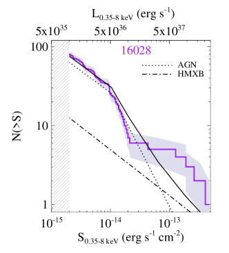
Figure 3.— The cumulative log$N$-log$S$ distribution for ObsID 16028. The shaded region shows the uncertainty in the number of observed sources. The gray-lined region indicates fluxes below our 90% completeness limit; only sources above this limit are shown. The left panel shows the predicted AGN, HMXB, and LMXB contributions based on log$N$-log$S$ distributions in the literature. The right panel shows the resulting fit when the normalizations are left as free parameters (e.g., the LMXB normalization is consistent with zero). See Section 3.1 for further discussion.

All fitting of the log$N$-log$S$ distributions was performed using Sherpa (version 1 for CIAO 4.8; Freeman et al., 2001; Doe et al., 2007) . There are two approaches to fitting the log$N$-log$S$ distributions: one can either fit the differential distribution (which may be biased by choice of binning scheme) or the cumulative distribution (which is not straightforward as the errors in each bin are correlated). In our analysis, we fit the differential distributions using the maximum-likelihood based cstat ($C$) statistic and the neldermead optimization method. Parameter uncertainties were measured using pyBLoCXs, a Markov chain Monte Carlo-based algorithm, written in Python, designed to carry out Bayesian analysis in the Sherpa environment using the “MetropolisMH” sampler and 10⁴ draws. Lower bounds were set at the 16th percentile value and upper bounds were set to the 84th value. Each free parameter was assigned a Gaussian prior centered at the best-fit value and a FWHM set by the 1.6$\sigma$ ($\sim$90% confidence) range returned by the covariance function. There is no difference between the fit parameters that we report and those that are obtained with only the differential log$N$-log$S$ distributions, except for the size of the parameter uncertainties.

To account for incompleteness in our survey, we compute an ancillary response function (ARF) that was folded in with the log$N$-log$S$ model in Sherpa, as was done in a similar study of the Antennae (Zezas et al., 2007). Due to the low background and negligible diffuse X-ray emission from NGC 300, the ARF essentially contains the probability that a source of a given flux was detected in our survey. To calculate the ARF, we use the approach of Georgakakis et al. (2008); we summarize the method here, and the reader is referred to their Section 4 for further details. Source extraction algorithms, such as wavdetect, estimate the probability that the observed number of counts within a detection cell arise from random fluctuations above the background level. Each cell contains counts from the background and possibly a source. Background images were produced using the CIAO task flux_image with point sources masked, and we calculate the Poisson probability in each cell in our image that the observed number of counts could fluctuate above $L$, the minimum number of counts for a formal detection (see Georgakakis et al., 2008, their equation 3). The faintest source included in our survey (e.g., that made the $>$3.5$\sigma$ cut, as described in Section 2.1) contained $\sim$5 counts in the 0.35-8 keV band. We therefore use $L=5$, and assume each source has a power law spectral shape with $\Gamma=1.7$. Figure 2 shows the cumulative probability that a source with a given flux would be detected in our shallowest exposure (e.g., the ARF).

We fit the three observations of the log$N$-log$S$ distribution using two physically motivated models: first, using the well-studied HMXB and LMXB XLFs (along with a background AGN component); second, we separate the X-ray sources on the basis of their temporal properties (persistent vs. variable sources, with a background AGN component).

3.1. Model I: AGN + HMXBs + LMXBs

The total X-ray luminosity from a galaxy (due to the discrete X-ray sources) is given by $L_{X}=\alpha$M${}_{*}+\beta$SFR, where the coefficients $\alpha$ and $\beta$ have been measured by Lehmer et al. (2010). HMXBs dominate the X-ray output when the SFR/M_∗ of the host galaxy is $\gtrsim$5.9$\times 10^{-11}$ yr^-1 (Lehmer et al., 2010). NGC 300 has a SFR of $\sim$0.15 $M_{\odot}$ yr^-1 (Gogarten et al., 2010) and a stellar mass of $\sim$2$\times 10^{9}$ $M_{\odot}$ (Muñoz-Mateos et al., 2007), which yields a SFR/M_∗ ratio just over the HMXB-dominant threshold. Using the Lehmer et al. (2010) coefficients predicts $L_{\rm X,HMXB}\sim 2.4\times 10^{38}$ erg s^-1 and $L_{\rm X,LMXB}\sim 1.8\times 10^{38}$ erg s^-1.

Table 2Measured Differential log$N$-log$S$ Components from the Literature

Component	$K^{a}$	$S_{\rm b}$ (10-14 erg s-1 cm-2)	$\gamma_{\rm f}$	$\gamma_{\rm b}$	Predicted #b	Reference
(1)	(2)	(3)	(4)	(5)	(6)	(7)
AGN	395	1.05$\pm$0.16	1.55$\pm$0.18	2.46$\pm$0.08	37 (7)	Cappelluti et al. (2009)
LMXB	(4.6$\pm$1.3)/($10^{10}$ $M_{\odot}$)	11.7${}^{+3.5}_{-4.9}$	1.1${}^{+0.12}_{-0.13}$	2.4$\pm$0.5	4 (4)	Lin et al. (2015)c
HMXB	(1.49$\pm$0.07)$\times$SFR	2254${}^{+1168}_{-697}$	1.58$\pm$0.02	2.73${}^{+1.58}_{-0.54}$	$<$3	Mineo et al. (2012)

Table 3Best-Fit Normalizations for Model I

Component	Predicted #	ObsID
		12238	16028	16029
(1)	(2)	(3)	(4)	(5)
AGN	$\sim$63-80	32.3${}^{+4.7}_{-4.6}$	26.1${}^{+6.7}_{-6.0}$	33.1${}^{+6.6}_{-7.7}$
LMXB	$<$4	$<$2.6	$<$3.5	$<$2.7
HMXB	$\sim$17-32	$<$6.5	$<$12.4	$<$11.4

We first attempted to model the NGC 300 log$N$-log$S$ distribution as the sum of three components (hereafter referred to as Model I): an AGN component, an HMXB component, and an LMXB component. All three components have had their log$N$-log$S$ distributions separately modeled by numerous authors as broken power laws with the general (differential) form

$$\frac{dN}{dS}=\begin{cases}KS^{-\gamma_{\rm f}},&S<S_{\rm b}\\ KS_{\rm b}^{\gamma_{\rm b}-\gamma_{\rm f}}S^{-\gamma_{\rm b}},&S>S_{\rm b}.\end{cases}$$ (5)

The values of normalization constants $K$, break fluxes $S_{\rm b}$, and the faint- and bright-end slopes ($\gamma_{\rm f}$ and $\gamma_{\rm b}$, respectively) are summarized in Table LABEL:table_physical_models. The high-luminosity break in the HMXB XLF near $\sim 10^{40-41}$ erg s^-1 (e.g., $\sim$10^-11 erg s^-1 cm^-2) has been observed by other authors (Grimm et al., 2003; Jeltema et al., 2003) for galaxies with especially high SFRs. NGC 300 does not contain such luminous X-ray sources; the brightest X-ray source, NGC 300 X-1, has a luminosity of $\sim$4$\times 10^{38}$ erg s^-1 (Binder et al., 2011, 2015). We therefore use a high-luminosity cut-off of 10⁴¹ erg s^-1 for the HMXB XLF. We use the Lin et al. (2015) XLF for field LMXBs in NGC 3115 (as opposed to those found in globular clusters), which reaches a similar depth to our own observations. Other studies of the XLF of field LMXBs in early-type galaxies (e.g., Kim et al., 2009; Lehmer et al., 2014; Peacock & Zepf, 2016) and have yielded similar fit parameters. Accounting for the variance in the reported field LMXB XLFs yields an additional $\sim$30% uncertainty in the number of LMXBS in NGC 300. Contamination from LMXBs in globular clusters is expected to be minimal, as the NGC 300 disk has been imaged multiple times by the Hubble Space Telescope, as discussed in Binder et al. (2012).

The measured AGN source density of $\sim$480 deg^-2 (Cappelluti et al., 2009) predicts $\sim$37 AGN in our survey area. We can use the HMXB and LMXB log$N$-log$S$ distributions to estimate the number of expected HMXBs and LMXBs be present in our survey. The normalizations for the HMXB and LMXB XLFs are correlated with the SFR and stellar mass of the host galaxy, respectively (Mineo et al., 2012; Lin et al., 2015); assuming a SFR of $\sim$0.15 $M_{\odot}$ yr^-1 and a stellar mass of $\sim$2$\times 10^{9}$ $M_{\odot}$ for NGC 300 (Muñoz-Mateos et al., 2007) yields $K_{\rm HMXB}\sim 0.22$ and $K_{\rm LMXB}\sim 0.92$. Integrating the differential log$N$-log$S$ distributions for these two components predicts $<$3 HMXBs and $\sim$4 LMXBs above the flux limit of our survey. These estimates suggest that $\sim$84%, 7%, and 9% of X-ray sources in NGC 300 will be AGN, HMXBs, and LMXBs, respectively. The predicted number of X-ray sources ($\sim$44) is a factor of $\sim$2 lower than the observed number of X-ray sources, with the largest discrepancy likely originating in the predicted number of HMXBs (see, e.g. Binder et al., 2012; Williams et al., 2013). We note that the shapes of the HMXB and LMXB XLFs have been derived using galaxies with systematically brighter X-ray point source populations than NGC 300; the other galaxy nearby galaxy with a well-studied, faint X-ray source population is the SMC, which also shows an HMXB excess. Although this excess has been attributed to a burst of recent star formation and low metallicity, low-intensity X-ray variability may be a contributing factor (see next section).

A cumulative power law distribution of the form $N(>S)\propto S^{-\gamma}$ will have a corresponding $dN/dS\propto S^{-\gamma-1}$, which is also a power law; the cumulative power law index $\gamma_{\rm c}$ is related to the differential power law index $\gamma_{\rm d}$ such that $\gamma_{\rm d}=\gamma_{\rm c}+1$. We fit the differential log$N$-log$S$ distributions using the same model (bpl1d + bpl1d + powlaw1d in Sherpa), with the power law indices and break fluxes frozen at the values listed in Table LABEL:table_physical_models. Only the normalization of each component was left as a free parameter.

The best-fit normalizations for Model I are summarized in Table LABEL:table_ModelI_norms. The log$N$-log$S$ distribution for ObsID 16028 is shown in Figure 3 with both the predicted log$N$-log$S$ distribution (based on the parameters in Table LABEL:table_physical_models) and the best-fit Model I superimposed; fits to the other two ObsID distributions are similar. These normalizations predict that $\sim$64-80% of X-ray sources are AGN, $\sim$2-4% are LMXBs, and $\sim$17-32% are HMXBs. This model does not adequately match the observed log$N$-log$S$ distributions; typically, $\chi^{2}$/dof $\sim 270/71$, while the $Q$-value (the probability that one would observe the reduced statistic value, or a larger value, if the assumed model is true) returned $\sim$0 for all three observations. We therefore consider a different model for the shape of the log$N$-log$S$ distribution that can be tested with our multiple exposures of NGC 300: one in which sources are separated by their temporal variability properties.

3.2. Model II: AGN + Persistent XRBs + Variable XRBs

Given the detection of variability in the shape of the log$N$-log$S$ distribution, we next consider whether the NGC 300 X-ray point source population can be characterized by the variability properties of the XRBs instead of by the mass of their companion donor star. Both HMXB and LMXB systems exhibit X-ray variability, and both types of systems accrete via the same basic mechanisms. Systems with persistently high X-ray luminosities (above $10^{35}$ erg s^-1) are produced when the radius of the donor star fills its Roche lobe, and mass transfer to the compact object becomes dominated by the tidal stream between the two components (e.g., Roche lobe overflow, RLOF). Although these sources can achieve luminosities up to $\sim$10⁴⁰ erg s^-1, lower luminosities of a few $10^{36}$ erg s^-1 are frequently observed in Galactic sources (e.g., Vela X-1; see Walter et al., 2015, and references therein) and in SMC pulsar-HMXBs (Laycock et al., 2010). However, most XRBs in the Milky Way and SMC produce very low X-ray luminosities ($\sim$10³³ erg s^-1). Instead of undergoing RLOF, the compact objects in these systems capture only a small fraction of their companion star’s wind and, therefore, have very low accretion rates (Bondi & Hoyle, 1944; Davidson & Ostriker, 1973; Lamers et al., 1976; Liu et al., 2006; Laycock et al., 2005). There is some evidence that the XLF of Galactic wind-fed systems may follow a broken power law distribution, with sources below $\sim 2.5\times 10^{36}$ erg s^-1 following a flatter power law index (differential $\gamma\sim 1.4$, at $\sim$2$\sigma$ significance; Lutovinov et al., 2013).

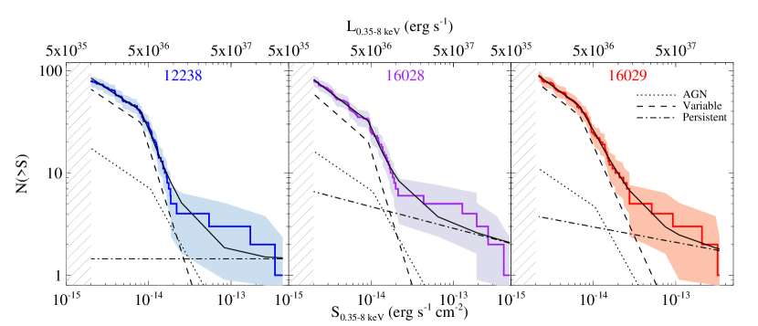
Figure 4.— The cumulative log$N$-log$S$ distributions derived for each ObsID. The best-fit model is superimposed (solid black line). The AGN, variable, and persistent components are shown by the dotted, dashed, and dot-dashed lines, respectively. The gray-lined region indicates fluxes below our 90% completeness limit; only sources above this limit are shown.

Table 4Best-Fit log$N$-log$S$ Distribution Parameters

Obs ID	$K_{\rm AGN}$	Persistent Component			Variable Component				$\chi^{2}$/dofb	Predicted # of Sources
		$K$	$\gamma$		$K$	$S_{\rm b}^{a}$	$\gamma_{\rm f}$	$\gamma_{\rm b}$		AGN	Persistent	Variable
(1)	(2)	(3)	(4)		(5)	(6)	(7)	(8)	(9)	(10)	(11)	(12)
12238	8.5${}^{+4.2}_{-4.3}$	0.7$\pm$0.4	1.3$\pm$0.1		14.6${}^{+2.1}_{-2.2}$	0.9$\pm$0.1	1.6$\pm$0.2	4.9${}^{+1.3}_{-1.2}$	59/69	21${}^{+10}_{-11}$	4$\pm$2	42$\pm$14
16028	8.4${}^{+4.5}_{-4.7}$	1.4${}^{+0.5}_{-0.6}$	$<$1.2		12.0${}^{+2.1}_{-2.0}$	0.9$\pm$0.1	1.8${}^{+0.2}_{-0.3}$	2.8${}^{+1.8}_{-0.8}$	48/67	20$\pm$11	9${}^{+3}_{-4}$	44${}^{+30}_{-17}$
16029	6.7$\pm$4.4	0.9$\pm$0.4	$<$1.2		17.6${}^{+2.7}_{-2.0}$	0.7$\pm$0.1	1.7$\pm$0.2	3.5$\pm$1.1	43/76	16$\pm$11	6$\pm$3	55${}^{+22}_{-21}$

High X-ray luminosities in non-RLOF HMXBs systems are produced in outbursts, which can be classified into Types I and II. Type I outbursts, which can reach luminosities of $\sim$10³⁷ erg s^-1, typically corresponding to the periastron passage of a NS in an eccentric orbit about its companion. As the NS enters the denser portions of the stellar wind close to periastron, the accretion rate increases and produces a predictable increase in the observed X-ray luminosity. Type II outbursts are somewhat fainter, $\sim 10^{36-37}$ erg s^-1, and can last from minutes to several orbital periods. These types of outbursts are frequently observed in supergiant HMXBs (see Reig, 2008; Ducci et al., 2014, and references therein), and the so-called supergiant fast X-ray transient (SFXT, Negueruela et al., 2008) events are shorter X-ray flares that occur as part of much longer outburst events, which can last several days (Sidoli et al., 2008; Romano et al., 2011, 2014a). The mechanism by which Type II outbursts and SFXT flares are produced is not certain, although eruptions from the donor star or changes in the stellar wind properties may contribute to the observed X-ray variability (Ducci et al., 2014, and references therein). LMXBs also exhibit strong X-ray variability, which is frequently accompanied by spectral changes that are driven by the structure of the inner accretion disk (Lewin et al., 1997; Maccarone, 2003; Asai et al., 2012).

We modeled the NGC 300 log$N$-log$S$ distribution as the sum of an AGN component (as in the previous section), a persistent XRB component (assumed to be a simple power law), and a variable XRB component. The variable component was modeled as a broken power law, as we anticipate a sharp decline in the number of observed sources above the typical outburst luminosity. The average AGN variability amplitude is $\sim$25-30% (Soldi et al., 2014), which is comparable to our flux uncertainties, particularly at the faint end; thus, we assume the background AGN contribution to our observed X-ray point sources is constant. The best-fit log$N$-log$S$ models are shown in Figure 4, and a visual comparison of the best-fit parameters is shown in Figure 5.

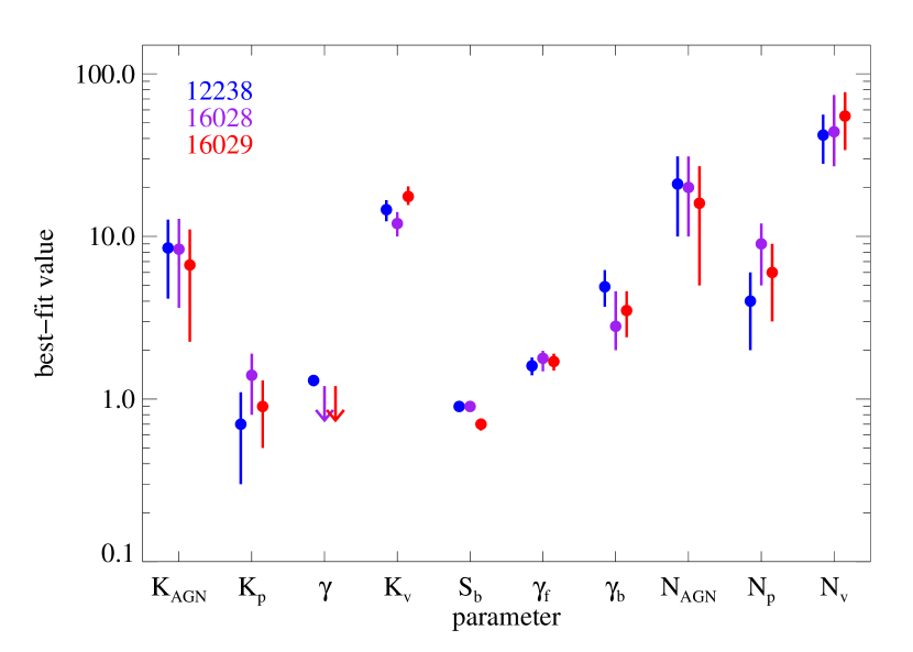
Figure 5.— Best-fit parameters, and the predicted number of sources, to the log$N$-log$S$ distributions for each ObsID.

Model II is a significantly better description than Model I of the log$N$-log$S$ distributions in all three observations; an F-test indicates that the improvement is significant at the $\sim$10$\sigma$ level. We note that the power law index and the predicted number of persistent sources is similar to the expected LMXB population. The power law index for the persistent component is $\lesssim$1.3, compared to an expected LMXB faint-end $\gamma_{\rm c}\sim 1-1.2$. A similar result is found for variable sources and HMXBs: the faint-end of the variable broken power law model has a $\gamma_{\rm f}\sim 1.6-1.8$, similar to $\gamma_{\rm c}\sim 1.6$ for the HMXB XLF. This result suggests that LMXBs may be, as a population, more persistent X-ray emitters (at least over the flux range sampled by our survey), while HMXBs show a greater degree of variability.

3.3. Persistent vs. Variable Sources

The NGC 300 log$N$-log$S$ distribution is best described as a combination of persistently bright XRBs and AGN and variable XRBs. To examine the contribution of these two populations to the overall log$N$-log$S$ distribution, we divided our sample into two categories: “persistent” sources that were detected in all three observations and did not show a flux change of more than a factor of two (within the flux uncertainties), and “variable” sources that either were detected in all observations but showed more than a factor of two change in flux, or were not detected in at least one observation but had a flux more than a factor of two above the 90% limiting flux in a different observation. We found 31 sources met our “persistent” criteria, and 41 sources were classified as “variable.” This is roughly consistent with the predicted number of persistent ($\sim$20–27) and variable ($\sim$33–49) sources from the previous section, as AGN are expected to meet this definition of “persistent.” The remaining 13 sources in the common area of our observations had unknown or ambiguous variability properties (e.g., they did not exceed a factor of two above the 90% limiting flux in one or two observation in which they were not detected) and so were not used in this analysis. A discussion of the log$N$-log$S$ distribution properties as a function of degree of variability is presented in the next subsection.

The 0.35-8 keV log$N$-log$S$ distributions were calculated in each epoch for the persistent and variable sources. There are three ways these distributions may be compared to one another: the persistent source distributions across all three epochs, the variable source distributions across all three epochs, and the persistent vs. variable source distributions within a single epoch. There is marginal evidence that the persistent source log$N$-log$S$ distributions vary across all three epochs; the minimum KS probability was 10% between ObsID 16028 and 16029. However, the variable source logN-logS distributions show significant differences between observations: the KS probability is $\lesssim$1.4% for all three combinations of epochs. Table 5 summarizes the KS probabilities for the log$N$-log$S$ distributions for all sources, persistent sources, and variable sources between observations. The probability that the persistent source distribution and the variable source distribution were drawn from the same underlying distribution within a single observation was also calculated and found to be $<0.05\%$ for all three observations. We can therefore say with confidence that the persistent X-ray sources in NGC 300 have fundamentally different population properties than the variable sources.

Table 5K-S Test Probabilities: By ObsID

ObsID	All Sources			Persistent			All Variable
	16028	16029		16028	16029		16028	16029
12238	0.87	0.28		0.96	0.55		0.0016	0.0039
16028	1	0.02		1	0.10		1	0.0135

Both distributions were initially fit as a three-component model: the AGN component, a broken power law (the variable component), and a simple power law (the persistent component), as in the previous section. When this model was applied to the persistent source distribution, the normalization of the variable component was consistent with zero. Likewise, the normalizations of the AGN and persistent components were both consistent with zero when we attempted to fit the variable sources with a three-component model. That the AGN component normalization was consistent with zero is not surprising. Studies of AGN variability as a function of flux (e.g., Paolillo et al., 2004) suggest that only $\sim$10% of AGN with $<$100 net counts (i.e., the majority of our sample) would exhibit X-ray flux variations significant enough to be considered “variable” in our study. We therefore removed these components and re-fit the distributions with the simplified versions of the model. The best-fit parameters found in both cases were nearly identical, but the simplified models yielded smaller uncertainties on the fit parameters; for example, typical uncertainties for the persistent source fit parameters were $\sim$19% when fitting three components, but $\sim$11% when fitting with two. F-tests between the simplified model and those with additional components yielded probabilities of $\sim$50–99%, indicating the additional components did not improve the quality of the fits. The results are shown in Figure 6, and the best-fit parameters are summarized in Table LABEL:table_fits_per_var.

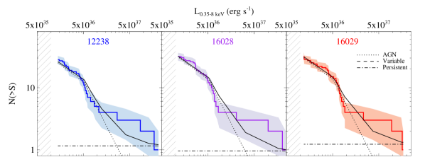
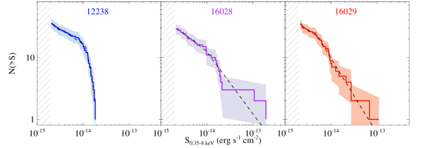
Figure 6.— The cumulative log$N$-log$S$ distributions of persistent sources (top) and variable sources (bottom). The AGN, variable, and persistent components are shown by the dotted, dashed, and dot-dashed lines, respectively. The persistent sources were fit with AGN and persistent components (the solid black line shows the sum of the components), while the variable sources were fit only with a variable component. ObsID 16028 shows the greatest similarity in the log$N$-log$S$ distributions between persistent and variable sources. The gray-lined region indicates fluxes below our 90% completeness limit; only sources above this limit are shown.

Table 6Best-Fit Persistent & Variable Source log$N$-log$S$ Distribution Parameters

Source	Obs ID	$K_{\rm AGN}$	Persistent Component			Variable Component				$\chi^{2}$/dofb	Predicted # of Sources
Type			$K$	$\gamma$		$K$	$S_{\rm b}^{a}$	$\gamma_{\rm f}$	$\gamma_{\rm b}$		AGN	Persistent	Variable
(1)	(2)	(3)	(4)	(5)		(6)	(7)	(8)	(9)	(10)	(11)	(12)	(13)
Persistent	12238	12.5${}^{+1.8}_{-1.0}$	0.4$\pm$0.2	$<$1.4		…	…	…	…	35/23	30${}^{+5}_{-2}$	2$\pm$1	…
	16028	13.7${}^{+1.3}_{-0.9}$	0.4$\pm$0.2	$<$1.5		…	…	…	…	43/26	33${}^{+4}_{-2}$	2$\pm$1	…
	16029	13.7${}^{+1.0}_{-1.3}$	0.4$\pm$0.2	$<$1.5		…	…	…	…	27/26	33$\pm$3	2$\pm$1	…
Variable	12238	…	…	…		11.5${}^{+1.5}_{-1.6}$	1.2$\pm$0.1	1.4$\pm$0.2	5.7${}^{+1.6}_{-2.8}$	13/30	…	…	30${}^{+11}_{-16}$
	16028	…	…	…		7.3${}^{+2.7}_{-2.2}$	0.9${}^{+0.2}_{-0.5}$	1.5$\pm$0.3	2.1${}^{+0.6}_{-0.5}$	16/23	…	…	25${}^{+14}_{-18}$
	16029	…	…	…		13.8${}^{+5.3}_{-3.5}$	0.5$\pm$0.3	1.3${}^{+0.5}_{-0.2}$	2.3${}^{+1.2}_{-0.7}$	17/29	…	…	30${}^{+29}_{-22}$

The persistent source distribution is dominated by the AGN component, which predicts $\sim$33 AGN within the common area of our survey. This is roughly consistent with the number we expect ($\sim$37) given the Cappelluti et al. (2009) AGN source density. The variable source distribution, on the other hand, is unlikely to have significant contamination by AGN. The low number of persistent sources intrinsic to NGC 300 ($\sim$2) and the power law slope ($<1.4$) is similar to the field LMXB XLF (Lin et al., 2015). This component is needed to explain the bright-end of the observed log$N$-log$S$ distributions, which is dominated by the bright source NGC 300 X-1 (Binder et al., 2011, 2015, and references therein). Although previously thought to be a Wolf Rayet + black hole HMXB, recent observations by Binder et al. (2015) have suggested that the donor star may be significantly less massive than previously believed, making X-1 a persistently bright black hole-LMXB.

The best-fit parameters for the persistent source distributions are also similar to those that were found for the persistent component in Section 3.2. The component normalization, break fluxes, and bright end power law indices for the variable sources exhibit more significant variation between exposures. The break fluxes ObsID 12238 and 16028 are similar, $\sim 9\times 10^{-15}$ erg s^-1 cm^-2 vs. $\sim 1.2\times 10^{-14}$ erg s^-1 cm^-2, respectively, but quite different from the $\sim 5\times 10^{-15}$ erg s^-1 cm^-2 found in ObsID 16029. Despite the differences in break flux, however, ObsID 16028 and 16029 have very similar bright-end power law indices (2.1 and 2.3, respectively). This difference in the bright-end slope from ObsID 12238 ($\gamma_{\rm b}\sim$5.7) is a consequence of a small number of bright sources observed in ObsIDs 16028 and 16029. Interestingly, the most stable component of the variable source distribution is the faint-end power law index, which is $\sim$1.4 in all three exposures. The break fluxes correspond to luminosities of $\sim$(2–67)$\times 10^{36}$ erg s^-1 at the distance of NGC 300. These parameters are consistent with the low-luminosity, wind-fed Galactic HMXB XLF presented in Lutovinov et al. (2013), whose definition of “persistent” refers to a lack of rapid X-ray variability on the order of the exposure time, whereas we are considering variability over months and years. Although the number of variable sources is consistent with the expected number of HMXBs from Table LABEL:table_ModelI_norms, we cannot rule out the possibility that variable LMXBs are contributing to the observed log$N$-log$S$ distributions.

We use the best-fit log$N$-log$S$ distributions to estimate the total X-ray luminosity produced by variable sources and persistent sources that are intrinsic to NGC 300. To do this, we randomly select the number of sources described by each component, drawn from the range of expected number of sources in Table LABEL:table_fits_per_var (e.g., $\sim$30 sources). We then populate the best-fit power law (or broken power law) with this number of sources and calculate the resulting luminosity. We repeat this process 10⁴ times for each distribution to estimate the range in X-ray luminosity our models predict from NGC 300. The persistent sources are expected to produce a luminosity of (1.8${}^{+12.0}_{-1.5}$)$\times 10^{37}$ erg s^-1, while the variable sources collectively produce (2.5${}^{+10.7}_{-2.2}$)$\times 10^{38}$ erg s^-1. The large uncertainties in the persistent source luminosity is due to the small number of X-ray sources intrinsic to NGC 300 compared to AGN (e.g., $\sim$2 persistent XRBs are expected, compared to $\sim$30 AGN), while the uncertainties in the variable source luminosity is primarily driven by the large differences in observed $\gamma_{\rm b}$. Within the uncertainties, however, these luminosities are consistent with the predicted LMXB and HMXB luminosities.

3.4. Variability Subclasses

We next considered whether the degree of individual source variability influenced the shape of the log$N$-log$S$ distributions. The variable sources were separated into three subclasses: “low-level” variable sources showed flux variations more than a factor of two but less than a factor of four, and “intermediate” variable sources exhibited flux variations of more than a factor of four but less than a factor of ten. “Transient” sources were not detected in at least one exposure, but had a flux more than an order of magnitude above the 90% limiting flux in at least one observation or exhibited a change in flux greater than an order of magnitude. Table LABEL:table_variable_classes summarizes the definitions of our variable source classification scheme.

Table 7Categories of X-ray Variability

Class	Definition	# Sources
(1)	(2)	(3)
persistent	$S_{\rm max}/S_{\rm min}\leq 2$	31
low-level variable	$2<S_{\rm max}/S_{\rm min}\leq 4$	18
intermediate variable	$4<S_{\rm max}/S_{\rm min}<10$	12
transient	$S_{\rm max}/S_{\rm min}>10$;	11
	at least one non-detection

The log$N$-log$S$ distributions were computed for each category in each observing epoch (using the source flux measured in that epoch), and a broken power law was fit to the resulting distributions. The results are shown in Figure 7. The best-fit parameters are summarized in Table LABEL:table_fit_variable and shown in Figure 8. Although the uncertainties are large due to the small number of sources used in the fit, nearly all the log$N$-log$S$ distributions show faint-end power law indices consistent with $\sim$1.6. The typical break flux range of $\sim$(0.5–1.5)$\times 10^{-14}$ erg s^-1 cm^-2 corresponds to a luminosity range of $\sim$(2.4–7.3)$\times 10^{36}$ erg s^-1 at the distance of NGC 300.

\begin{overpic}[width=433.62pt,clip={true},trim=0.0pt 36.98866pt 0.0pt 0.0pt]{var24_bestfit.eps} \put(10.0,23.0){\large low level} \end{overpic}

\begin{overpic}[width=433.62pt,clip={true},trim=0.0pt 36.98866pt 0.0pt 54.06006pt]{var49_bestfit.eps} \put(10.0,23.0){\large intermediate} \end{overpic}

\begin{overpic}[width=433.62pt,clip={true},trim=0.0pt 0.0pt 0.0pt 54.06006pt]{transient_bestfit.eps} \put(10.0,27.0){\large transient} \end{overpic}

Figure 7.— The cumulative log$N$-log$S$ distributions for each ObsID for low-level variable sources (top row), intermediate variables (middle row), and transient sources (bottom row). The best-fit model is shown by the solid black line. The gray-lined region indicates fluxes below our 90% completeness limit; only sources above this limit are shown.

Table 8log$N$-log$S$ Distribution Fits for Variable Source Subclasses

Category	Obs ID	$K$	$S_{\rm b}^{a}$	$\gamma_{\rm f}$	$\gamma_{\rm b}$	$\chi^{2}$/dofb
(1)	(2)	(3)	(4)	(5)	(6)	(7)
low-level	12238	4.3${}^{+1.0}_{-0.9}$	1.1${}^{+1.5}_{-0.7}$	1.5$\pm$0.2	4.8${}^{+2.9}_{-2.4}$	5/13
	16028	3.8$\pm$0.8	1.2${}^{+2.4}_{-0.4}$	1.6${}^{+0.2}_{-0.4}$	4.0${}^{+4.9}_{-2.1}$	7/8
	16029	6.0${}^{+3.2}_{-2.5}$	0.5${}^{+0.5}_{-0.4}$	1.6${}^{+0.4}_{-0.3}$	3.2${}^{+1.0}_{-0.7}$	4/13
intermediate	12238	4.0${}^{+1.3}_{-1.2}$	0.9${}^{+2.1}_{-0.3}$	$<$1.5	4.2${}^{+2.5}_{-1.7}$	2/5
	16028	2.6${}^{+0.9}_{-0.8}$	1.4${}^{+1.8}_{-0.5}$	1.8$\pm$0.4	2.0${}^{+2.2}_{-0.9}$	6/6
	16029	2.0$\pm$1.2	0.7${}^{+0.7}_{-0.3}$	1.6$\pm$0.4	2.0${}^{+2.5}_{-0.6}$	2/4
transient	12238	3.7${}^{+1.9}_{-1.2}$	0.7${}^{+1.4}_{-0.4}$	1.6${}^{+0.4}_{-0.5}$	5.8${}^{+2.4}_{-3.7}$	3/5
	16028	$<$4.4	1.1${}^{+1.6}_{-0.7}$	1.9${}^{+0.8}_{-0.6}$	6.2${}^{+3.2}_{-2.4}$	1/1
	16029	3.2${}^{+2.7}_{-2.1}$	0.6${}^{+1.0}_{-0.5}$	1.4${}^{+0.4}_{-0.2}$	2.6${}^{+1.8}_{-1.9}$	2/6

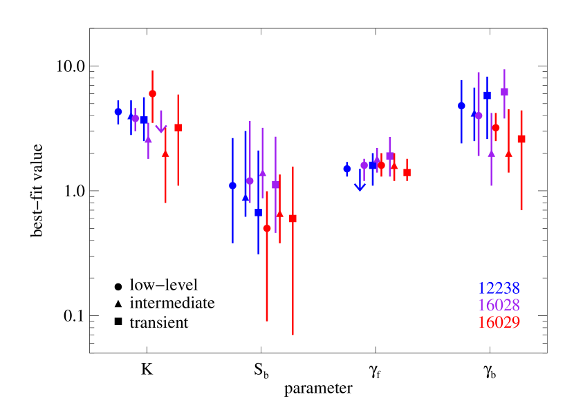
Figure 8.— Best-fit parameters obtained for our fits to the log$N$-log$S$ distributions for each ObsID and each variability category.

Two-sided K-S tests of the log$N$-log$S$ distributions between observations did not reveal any evidence for differences within the variability subclasses – the low-level variable sources in ObsID 12238 look, statistically, like the low-level variable sources in ObsID 16029. Table 9 provides the K-S test results for all ObsID combinations. We next compared the different variability categories within a single observation (i.e., we tested if the persistent sources in ObsID 12238 differed significantly from the transient sources in the same observation). The results are summarized in Table 10. There is significant evidence that the persistent X-ray sources are different from all categories of variable sources. However, there is no evidence that the different categories of variable sources differ from one another, which suggests that all types of variable X-ray sources are part of the same underlying population.

Table 9Variable Distribution K-S Test Probabilities: By ObsID

ObsID	Low-Level			Intermediate			Transient
	16028	16029		16028	16029		16028	16029
12238	0.99	0.92		0.99	0.99		0.99	0.22
16028	1	0.68		1	0.70		1	0.12

Table 10K-S Test Probabilities: Within Each ObsID

Class	low level	intermediate	transient
	12238
persistent	1.9$\times 10^{-5}$	2.8$\times 10^{-5}$	0.0025
low level	1	0.99	0.36
intermediate	…	1	0.62
	16028
persistent	2.2$\times 10^{-6}$	2.9$\times 10^{-5}$	0.0026
low level	1	0.99	0.14
intermediate	…	1	0.30
	16029
persistent	0.0004	2.9$\times 10^{-5}$	3.8$\times 10^{-6}$
low level	1	0.44	0.53
intermediate	…	1	0.99

4. Discussion

4.1. Modeling the XLF of Variable Sources

XRBs are intrinsically variable objects, and yet the resulting log$N$-log$S$ distributions constructed for an entire population of XRBs appear to follow a similar shape. We next considered whether the X-ray variability properties of these sources – such as the peak flux during an X-ray outburst or the frequency of the outbursts – could explain the shape of the observed log$N$-log$S$ distributions. The high-energy light curves of variable XRBs have been studied extensively using RXTE, BeppoSAX, Integral, Suzaku, and Swift, especially for Galactic sources (see, e.g. Reig & Nespoli, 2013; Reig, 2011; Stroh & Falcone, 2013) and in the SMC (Laycock et al., 2005). Generally, the shapes of these light curves fall into one of two generic classes: a smooth increase and subsequent decrease in the observed flux that broadly resembles a Gaussian curve, or a fast rise in X-ray flux followed by an exponential decay (Reig, 2011; Reig & Nespoli, 2013). We refer to these as “Gaussian” and fast rise exponential decay (“FRED”) profiles, respectively, for the remainder of this work.

Our aim was to generate a population of synthetic XRBs (some of which followed a Gaussian profile, and some of which followed a FRED profile), and then to “observe” these synthetic sources and construct log$N$-log$S$ distributions in exactly the same manner as was done for our Chandra observations. All synthetic sources were given a “quiescent” X-ray flux of $2\times 10^{-17}$ erg s^-1 cm^-2, equivalent to $\sim$10³³ erg s^-1 at the distance of NGC 300. The model light curves were described by three free parameters: the duration of time in between outbursts (hereafter referred to as the “duration”), the fraction of time that the source spends above the 90% limit flux of our observations (hereafter referred to as the “bright fraction”), and the peak flux. Peak fluxes were randomly drawn from a power law distribution of fluxes above the detection limit of our survey ($\sim 10^{36}$ erg s^-1), with the highest possible flux of $2\times 10^{-12}$ erg s^-1 cm^-2 (equivalent to 10³⁹ erg s^-1). The power law index of this distribution was our free parameter. Two template burst profiles are shown in Figure 9.

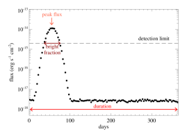
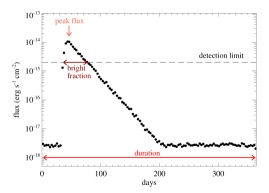
Figure 9.— Example light curve templates showing the Gaussian profile (left) and FRED profile (right). Our observational detection limit is shown by the horizontal dashed line. The duration, bright fraction, and peak flux are the model parameters that can be adjusted.

In order to determine what effect the free parameters in our profiles had on the resulting log$N$-log$S$ distributions, we generated a grid of 145 models: 125 of these used a roughly 50/50 mix of Gaussian and FRED profiles, and ten of these models were randomly selected and re-run two additional times, once using exclusively Gaussian profiles and once using exclusively FRED profiles, to generate the log$N$-log$S$ distributions. The duration parameter could have a value of 122, 183, 365, 730, or 1095 days (corresponding to a burst frequency of once per four months, six months, one year, two years, or three years), the bright fraction was set to 1%, 10%, 30%, 50%, or 70%, and the power law index that determined the distribution from which the peak flux was drawn could have a value of 0.6 (i.e., relatively flat distribution, indicating that bright bursts are somewhat likely to occur), 1.8, 2.6, 3.0, or 3.4 (i.e., steep distributions indicating a strong preference for fainter peak fluxes). While XRBs have been observed undergo outbursts on timescales less than 122 days, the time between our observations is too long for us to place any meaningful constraints on duration parameters this short. The bright fraction is related to the X-ray source duty cycle and the number of observations; typical duty cycles of XRBs are $\sim$20–60% (Romano et al., 2014b), but with our three observations we are not able to reliably test this currently-accepted range. For each model, 500 synthetic X-ray sources were created and three random fluxes were drawn from their light curves. Fluxes were assigned a $\sim$10-25% uncertainty, typical to the uncertainties of faint sources in our observations. The resulting synthetic log$N$-log$S$ distributions were then fit using a broken power-law in Sherpa in an identical manner as was done for the observed variable source distributions.

For each resulting fit, we record the best-fit values of $\gamma_{\rm f}$, $\gamma_{\rm b}$, and $S_{\rm b}$, and the corresponding uncertainties. We additionally performed a two-sided K-S test of each model against the observed variable source distributions. Models that returned very low K-S probabilities ($<$1%) for all three observations are not consistent with the observations. We found no significant difference in the resulting log$N$-log$S$ distributions or fit quality when only Gaussian or FRED profiles were used compared to the 50/50 mix. Table 11 summarizes the model parameters and resulting log$N$-log$S$ parameters for the five models that yielded K-S probabilities $>$5%. Figure 10 shows the bright fraction, duration, and burst power law index parameter space we explored; large circles show models with K-S probabilities $>$5% when compared to the observations, and the best-fit model is shown in green. The best-fit model was selected as the one with the highest K-S probability, and has a bright fraction of 1%, a duration of 122 days (corresponding to one outburst every $\sim$4 months), and a peak flux power law index of 3.0. This model yields log$N$-log$S$ fit parameters $\gamma_{\rm f}=1.5^{+0.3}_{-0.5}$, $\gamma_{\rm b}=3.0^{+0.5}_{-0.7}$, and $S_{\rm b}=(1.2^{+0.5}_{-0.6})\times 10^{-14}$ erg s^-1 cm^-2. Figure 11 provides three examples of log$N$-log$S$ distributions produced by our best-fit model, compared to the observed variable source distributions.

Table 11Best-Fit Synthetic Source Models

Bright	Burst Power	Duration	K-S	log$N$-log$S$ Best-Fit Parameters
Fraction (%)	Law Index	(days)	Probability	$\gamma_{\rm f}$	$\gamma_{\rm b}$	$S_{\rm b}^{a}$
(1)	(2)	(3)	(4)	(5)	(6)	(7)
1	0.6	122	0.05	1.7${}^{+0.5}_{-0.3}$	2.1${}^{+0.4}_{-0.6}$	1.7${}^{+0.7}_{-0.4}$
1	1.8	122	0.06	1.6$\pm$0.3	5.0${}^{+0.7}_{-0.5}$	0.8${}^{+0.6}_{-0.4}$
1	3.0	122	0.10	1.5${}^{+0.3}_{-0.5}$	3.0${}^{+0.5}_{-0.7}$	1.2${}^{+0.5}_{-0.6}$
1	3.4	122	0.09	1.6${}^{+0.5}_{-0.3}$	4.8${}^{+1.3}_{-0.6}$	0.8${}^{+0.6}_{-0.4}$
50	3.0	183	0.06	1.7${}^{+0.5}_{-0.3}$	6.7${}^{+0.7}_{-0.8}$	1.1${}^{+0.3}_{-0.5}$

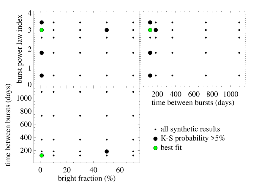
Figure 10.— The parameter space explored by our synthetic log$N$-log$S$ distributions. All model runs are shown by the small dots. Larger circles indicate models that yielded K-S probabilities $>$5%, and the green circle indicates our best-fit model.

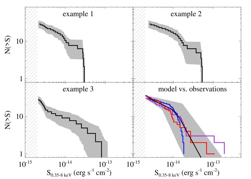
Figure 11.— Examples of the log$N$-log$S$ distributions produced by our best-fit variable source model. The bottom-right panel shows the best-fit model (black line, with uncertainties shown by the shaded gray region) compared to the observed variable source distributions. ObsID 12238 is shown in blue, 16028 is shown in purple, and 16029 is shown in red. The gray-lined region indicates fluxes below our 90% completeness limit; only sources above this limit are shown.

The observed log$N$-log$S$ distributions clearly favor models with X-ray sources that burst multiple times per year. The two best models additionally have small bright fractions, 1%, and steep burst power law indices, indicating that the majority of XRB bursts occur at relatively faint fluxes, and that bright X-ray bursts are severely underrepresented in our survey. Of the tens of thousands of synthetic X-ray sources generated, only $\sim$0.4% produced an “observed” peak flux above the Eddington limit of a 1.4 $M_{\odot}$ neutron star (2$\times 10^{38}$ erg s^-1), and they were all the result of the flatter (burst power law index of 0.6) peak flux distributions.

It is typically assumed that, during an outburst, an XRB produces a peak luminosity at or near its Eddington limit. We therefore generated synthetic light curves in which we required the peak flux to correspond to the Eddington limit of a 1.4 $M_{\odot}$ NS. The faint- and bright-end power law indices were similar to those found in our observations, but the break flux is a factor of $\sim$10 higher. The synthetic log$N$-log$S$ distributions have typical break fluxes from $\sim$5$\times 10^{-14}$ erg s^-1 cm^-2 to $\sim 10^{-13}$ erg s^-1 cm^-2, equivalent to $\sim$(2–5)$\times 10^{37}$ erg s^-1 at the distance of NGC 300, across all values of duration and bright fraction. The best K-S probability from the Eddington models was $\sim$5$\times 10^{-7}$, indicating a significant difference from the observations. These results therefore suggest that the majority of outbursting XRBs in NGC 300 occur at sub-Eddington luminosities.

4.2. X-ray Binary Variability and Evolution

The persistent sources in NGC 300 are likely dominated by background AGN, with a handful of RLOF LMXBs, while the variable source distribution is likely a mix of HMXBs and LMXBs, dominated by HMXBs, outbursting at sub-Eddington rates. Assuming a 1.4 $M_{\odot}$ NS, the typical variable source break flux corresponds to a luminosity of $\sim$(2–6)$\times 10^{36}$ erg s^-1 corresponds to an accretion rate of 1–3% the Eddington limit. Furthermore, we have modeled the log$N$-log$S$ distributions originating from outbursting X-ray sources, and found we can match the broken power law shape seen in our observations when the distribution of peak fluxes significantly favors faint outbursts. Although bright X-ray bursts are better studied, particularly in extragalactic sources, our results imply that they do not represent the “typical” X-ray variable source in NGC 300.

The faint-end of the variable source log$N$-log$S$ distribution has a power law index of $\sim$1.7, similar to the universal XLF of HMXBs. Recently, Zuo & Li (2014) suggested that the shape of the XLF could be explained by the common envelope (CE) evolution of the progenitor binary as it evolves. Their simulations were able to reproduce the observed XLF for two common formalisms of CE evolution: the $\alpha_{\rm CE}$ formalism (also called the “energy-budget” approach) and the $\gamma$-formalism (the “angular momentum” budget approach). In the $\alpha_{\rm CE}$ formalism, the CE evolution is parameterized in terms of the orbital energy ($E_{\rm orb}$) and the envelope binding energy ($E_{\rm bind}$). The parameter $\alpha_{\rm CE}$ describes the efficiency at which the system’s orbital energy is converted into kinetic energy that is used to eject the envelope (Webbink, 1984, 2008). Under the $\gamma$-formalism, CE evolution is instead parameterized by the ratio of the fraction of angular momentum lost during the CE phase and the fraction of mass loss in the system, and has been more successful in explaining the observed properties of double-white dwarf binaries, cataclysmic variables, and binary main sequence stars (Nelemans & Tout, 2005).

The simulated XRB populations in Zuo & Li (2014) included a large fraction of variable sources, including both NS and BH primaries with supergiant and Be companions undergoing either Roche lobe overflow or direct wind accretion. However, persistent and variable sources were not separated during the construction of the XLFs. The shapes of the simulated XLFs were similar for both CE evolution parameterizations, but the number of characteristics of the resulting HMXB populations were distinctly different from one another. Under the $\alpha_{\rm CE}$-formalism, XRBs with MS companions are the dominant source of X-rays below $10^{37}$ erg s^-1, while the XRBs with He-rich companions (e.g., evolved donors that have lost a significant fraction of their outer H envelopes) are the majority constituent under the $\gamma$-formalism. Our X-ray observations indicate that the variability properties of both HMXBs and LMXBs may contribute to the shape of the XLF independently of the evolutionary history of the system. Our X-ray observations are not adequate to determine which scenario is more likely for the low-luminosity X-ray sources in NGC 300.

5. Conclusions

We have studied the log$N$-log$S$ distributions of X-ray sources in NGC 300 across three epochs with Chandra down to $\sim$10³⁶ erg s^-1. This is an order of magnitude fainter than a similar study of the Antennae galaxies (Zezas et al., 2007). We find that the majority of variable X-ray sources in NGC 300 have luminosities less than $\sim 5\times 10^{36}$ erg s^-1, while the brightest sources exhibit persistent X-ray emission (within a factor of $\sim$2). This result may help explain why variable X-ray sources have not had a significant impact on studies of the XLF in single, “snapshot” exposures, as these observations frequently detect only sources above $\sim$10³⁷ erg s^-1. If all significantly variable X-ray sources are faint but numerous, as implied by our observations, then their large numbers would result in similar distributions of brightness across different observations.

The persistent sources in NGC 300 are likely undergoing mass transfer via RLOF, and their flat log$N$-log$S$ distribution is consistent with that of field LMXBs (Lin et al., 2015). However, the persistent source population is likely dominated by AGN, particularly at low fluxes ($\lesssim 2\times 10^{-14}$ erg s^-1 cm^-2). The variable source XLF is well described by a broken power law, with a faint-end power law index similar to that of HMXBs (Mineo et al., 2012) with cut-off fluxes of $\sim$(0.5–1.5)$\times 10^{-14}$ erg s^-1 cm^-2, corresponding to a luminosity of $\sim$(2–7)$\times 10^{36}$ erg s^-1. These observations suggest that the highly variable X-ray sources in NGC 300 are wind-accreting XRBs, possibly HMXBs undergoing Type II outbursts, although we cannot completely rule out a significant contribution from variable LMXBs to the shape of the highly variable log$N$-log$S$ distribution.

We were able to reproduce the observed log$N$-log$S$ distributions of variable sources in NGC 300 by assuming generic profiles of the X-ray outbursts, with no assumptions made about the prior evolutionary history of the systems. It is unclear to what degree the shape of the XLF is the result of CE evolution, and how much may be driven by the variability properties of the underlying source distribution. CE evolution likely plays a key role in determining the shape of the persistent-source XLF and determining the fraction of the massive binary population that later produces variable XRBs. A better understanding of how the X-ray outburst profiles are related to its prior evolutionary history may provide clues to the missing link between the variability properties of XRBs and the “universal” shape of the HMXB XLF; repeated Chandra observations of nearby, star-forming galaxies down to $\sim 10^{36}$ erg s^-1 are necessary to better constrain the XLF shape of outbursting and RLOF XRBs.

References

- Antoniou et al. (2010) Antoniou, V., Zezas, A., Hatzidimitriou, D., & Kalogera, V. 2010, ApJ, 716, L140
- Asai et al. (2012) Asai, K., et al. 2012, PASJ, 64
- Binder et al. (2015) Binder, B., Gross, J., Williams, B. F., & Simons, D. 2015, MNRAS, 451, 4471
- Binder et al. (2012) Binder, B., et al. 2012, ApJ, 758, 15
- Binder et al. (2011) Binder, B., Williams, B. F., Eracleous, M., Garcia, M. R., Anderson, S. F., & Gaetz, T. J. 2011, ApJ, 742, 128
- Bland-Hawthorn et al. (2005) Bland-Hawthorn, J., Vlajić, M., Freeman, K. C., & Draine, B. T. 2005, ApJ, 629, 239
- Bondi & Hoyle (1944) Bondi, H., & Hoyle, F. 1944, MNRAS, 104, 273
- Cappelluti et al. (2009) Cappelluti, N., et al. 2009, A&A, 497, 635
- Dalcanton et al. (2009) Dalcanton, J. J., et al. 2009, ApJS, 183, 67
- Davidson & Ostriker (1973) Davidson, K., & Ostriker, J. P. 1973, ApJ, 179, 585
- Doe et al. (2007) Doe, S., et al. 2007, in Astronomical Society of the Pacific Conference Series, Vol. 376, Astronomical Data Analysis Software and Systems XVI, ed. R. A. Shaw, F. Hill, & D. J. Bell, 543
- Ducci et al. (2014) Ducci, L., Doroshenko, V., Romano, P., Santangelo, A., & Sasaki, M. 2014, A&A, 568, A76
- Freeman et al. (2001) Freeman, P., Doe, S., & Siemiginowska, A. 2001, in Proc. SPIE, Vol. 4477, Astronomical Data Analysis, ed. J.-L. Starck & F. D. Murtagh, 76
- Freeman et al. (2002) Freeman, P. E., Kashyap, V., Rosner, R., & Lamb, D. Q. 2002, ApJS, 138, 185
- Gehrels (1986) Gehrels, N. 1986, ApJ, 303, 336
- Georgakakis et al. (2008) Georgakakis, A., Nandra, K., Laird, E. S., Aird, J., & Trichas, M. 2008, MNRAS, 388, 1205
- Gogarten et al. (2010) Gogarten, S. M., et al. 2010, ApJ, 712, 858
- Grimm et al. (2003) Grimm, H.-J., Gilfanov, M., & Sunyaev, R. 2003, MNRAS, 339, 793
- Jeltema et al. (2003) Jeltema, T. E., Canizares, C. R., Buote, D. A., & Garmire, G. P. 2003, ApJ, 585, 756
- Kalberla et al. (2005) Kalberla, P. M. W., Burton, W. B., Hartmann, D., Arnal, E. M., Bajaja, E., Morras, R., & Pöppel, W. G. L. 2005, A&A, 440, 775
- Kilgard et al. (2002) Kilgard, R. E., Kaaret, P., Krauss, M. I., Prestwich, A. H., Raley, M. T., & Zezas, A. 2002, ApJ, 573, 138
- Kim et al. (2004) Kim, D.-W., et al. 2004, ApJS, 150, 19
- Kim et al. (2009) Kim, D.-W., et al. 2009, ApJ, 703, 829
- Lamers et al. (1976) Lamers, H. J. G. L. M., van den Heuvel, E. P. J., & Petterson, J. A. 1976, A&A, 49, 327
- Larsen & Richtler (1999) Larsen, S. S., & Richtler, T. 1999, A&A, 345, 59
- Laycock et al. (2005) Laycock, S., Corbet, R. H. D., Coe, M. J., Marshall, F. E., Markwardt, C., & Lochner, J. 2005, ApJS, 161, 96
- Laycock et al. (2010) Laycock, S., Zezas, A., Hong, J., Drake, J. J., & Antoniou, V. 2010, ApJ, 716, 1217
- Lehmer et al. (2010) Lehmer, B. D., Alexander, D. M., Bauer, F. E., Brandt, W. N., Goulding, A. D., Jenkins, L. P., Ptak, A., & Roberts, T. P. 2010, ApJ, 724, 559
- Lehmer et al. (2014) Lehmer, B. D., et al. 2014, ApJ, 789, 52
- Lewin et al. (1997) Lewin, W. H. G., van Paradijs, J., & van den Heuvel, E. P. J. 1997, X-ray Binaries 674
- Lin et al. (2015) Lin, D., et al. 2015, ApJ, 808, 20
- Liu (2011) Liu, J. 2011, ApJS, 192, 10
- Liu et al. (2006) Liu, Q. Z., van Paradijs, J., & van den Heuvel, E. P. J. 2006, A&A, 455, 1165
- Lutovinov et al. (2013) Lutovinov, A. A., Revnivtsev, M. G., Tsygankov, S. S., & Krivonos, R. A. 2013, MNRAS, 431, 327
- Maccarone (2003) Maccarone, T. J. 2003, A&A, 409, 697
- McSwain & Gies (2005) McSwain, M. V., & Gies, D. R. 2005, ApJS, 161, 118
- Mineo et al. (2012) Mineo, S., Gilfanov, M., & Sunyaev, R. 2012, MNRAS, 419, 2095
- Muñoz-Mateos et al. (2007) Muñoz-Mateos, J. C., Gil de Paz, A., Boissier, S., Zamorano, J., Jarrett, T., Gallego, J., & Madore, B. F. 2007, ApJ, 658, 1006
- Negueruela et al. (2008) Negueruela, I., Torrejón, J. M., Reig, P., Ribó, M., & Smith, D. M. 2008, in American Institute of Physics Conference Series, Vol. 1010, A Population Explosion: The Nature & Evolution of X-ray Binaries in Diverse Environments, ed. R. M. Bandyopadhyay, S. Wachter, D. Gelino, & C. R. Gelino, 252
- Nelemans & Tout (2005) Nelemans, G., & Tout, C. A. 2005, MNRAS, 356, 753
- Paolillo et al. (2004) Paolillo, M., Schreier, E. J., Giacconi, R., Koekemoer, A. M., & Grogin, N. A. 2004, ApJ, 611, 93
- Peacock & Zepf (2016) Peacock, M. B., & Zepf, S. E. 2016, ApJ, 818, 33
- Reig (2008) Reig, P. 2008, A&A, 489, 725
- Reig (2011) Reig, P. 2011, Ap&SS, 332, 1
- Reig & Nespoli (2013) Reig, P., & Nespoli, E. 2013, A&A, 551, A1
- Romano et al. (2014a) Romano, P., Ducci, L., Mangano, V., Esposito, P., Bozzo, E., & Vercellone, S. 2014a, A&A, 568, A55
- Romano et al. (2014b) Romano, P., Guidorzi, C., Segreto, A., Ducci, L., & Vercellone, S. 2014b, A&A, 572, A97
- Romano et al. (2011) Romano, P., et al. 2011, MNRAS, 410, 1825
- Shtykovskiy & Gilfanov (2005) Shtykovskiy, P., & Gilfanov, M. 2005, MNRAS, 362, 879
- Shtykovskiy & Gilfanov (2007) Shtykovskiy, P. E., & Gilfanov, M. R. 2007, Astronomy Letters, 33, 437
- Sidoli et al. (2008) Sidoli, L., et al. 2008, ApJ, 687, 1230
- Soldi et al. (2014) Soldi, S., et al. 2014, A&A, 563, A57
- Stroh & Falcone (2013) Stroh, M. C., & Falcone, A. D. 2013, ApJS, 207, 28
- Walter et al. (2015) Walter, R., Lutovinov, A. A., Bozzo, E., & Tsygankov, S. S. 2015, A&A Rev., 23, 2
- Webbink (1984) Webbink, R. F. 1984, ApJ, 277, 355
- Webbink (2008) Webbink, R. F. 2008, in Astrophysics and Space Science Library, Vol. 352, Astrophysics and Space Science Library, ed. E. F. Milone, D. A. Leahy, & D. W. Hobill, 233
- Williams et al. (2013) Williams, B. F., Binder, B. A., Dalcanton, J. J., Eracleous, M., & Dolphin, A. 2013, ApJ, 772, 12
- Zezas et al. (2007) Zezas, A., Fabbiano, G., Baldi, A., Schweizer, F., King, A. R., Rots, A. H., & Ponman, T. J. 2007, ApJ, 661, 135
- Zuo & Li (2014) Zuo, Z.-Y., & Li, X.-D. 2014, ApJ, 797, 45