Projective measurement of energy on an ensemble of qubits with unknown frequencies

Abstract

In projective measurements of energy, a target system is projected to an eigenstate of the system Hamiltonian, and the measurement outcomes provide the information of corresponding eigen-energies. Recently, it has been shown that such a measurement can be in principle realized without detailed knowledge of the Hamiltonian by using probe qubits. However, in the previous approach for the energy measurement, the necessary size of the dimension for the probe increases as we increase the dimension of the target system, and also individual addresibility of every qubit is required, which may not be possible for many experimental settings with large systems. Here, we show that a single probe qubit is sufficient to perform such a projective measurement of energy if the target system is composed of non-interacting qubits whose resonant frequencies are unknown. Moreover, our scheme requires only global manipulations where every qubit is subjected to the same control fields. These results indicate the feasibility of our energy projection protocols.

A projective measurement is a central concept in quantum physics von Neumann (1932); Koshino and Shimizu (2005); Wiseman and Milburn (2009). This ideally projects the state to the eigenstate of the measured observable. The quantum measurement process can be described by an interaction between the target system and a probe system. A correlation with the probe system is generated via the coupling, and a measurement on the probe system induces the projection on the target system where the measurement outcomes of the probe are associated with the eigenvalues of the observable. If the measured observable is energy of the target system, such an operation is called projective measurement of energy (PME).

PME scheme exists if the form of the Hamiltonian is given in advance Aharonov et al. (2002). Based on the knowledge of the Hamiltonian, we can engineer the interaction between the target and probe system. However, to identify the unknown Hamiltonian, it takes at least $O(d^{2})$ time with quantum tomography where $d$ denotes the Hilbert space of the system Chuang and Nielsen (1997); Poyatos et al. (1997), and this grows exponentially with the size of the target system.

Nakayama et al proposed a scheme to perform the PME of unknown Hamiltonians whose dimension and energy scale are only known. The necessary time is independent from the dimension of the Hamiltonian Nakayama et al. (2015). Quantum phase estimation (QPE) algorithm is used to estimate eigenvalues of a given unitary operator $U$ Kitaev et al. (2002), and controlled-swap gates between the target system and probe system play a central role implementing the PME. However, there are no existing schemes to construct the controlled-swap gate in actual experiments when the Hamiltonian is unknown. Moreover, their protocol requires a probe system whose size is comparable with that of the target system, while individual controllability for every qubit is requisite. Due to these restrictions, it is not clear whether their protocol could be demonstrated in actual experiments.

In this letter, we introduce a scheme to implement the PME on an ensemble of qubits with unknown frequencies where only global control with a single probe qubit is required, while keeping the advantage of the reduced time cost. We consider that a single probe qubit is collectively coupled with the target qubits where interaction between the target qubits is negligible. Without detailed knowledge of the target qubits, one can perform the PME via the coupling with the probe qubit, while the necessary time cost is independent from the dimension of the Hamiltonian. Moreover, our protocol just requires global controls where all qubits are subjected in the same external fields. These advantages show our PME is much more suitable for experimental realizations than the previous schemes.

Let us review quantum phase estimation (QPE) Kitaev et al. (2002). Here, we consider the case that QPE is performed on a given unitary operation under the assumption that implementation of a controlled unitary gate and Fourier basis measurements are available. By QPE, we can estimate eigenvalues of a target unitary operator $U_{t}=e^{-iH_{\rm{QPE}}t}=\sum_{n=0}^{2^{N}-1}e^{-iE_{n}t}|E_{n}\rangle\langle E_{n}|$ where $|E_{n}\rangle$ and $E_{n}$ denote eigenvectors and eigenvalues of the target Hamiltonian $H_{\rm{QPE}}$, respectively. We assume $0\leq E_{n}t<2\pi$ $(n=1,2,\cdots,L)$ to remove an ambiguity due to a phase periodicity. A control-unitary operation $\mathcal{C}_{U_{t}}=|0\rangle_{\rm{P}}\langle 0|\otimes\openone_{\rm{T}}+|1\rangle_{\rm{P}}\langle 1|\otimes U_{t}$ between the probe qubit and the target qubits is required for the implementation of QPE. This operation can induce a phase kick back $\mathcal{C}_{U_{t}}|+\rangle_{\rm{P}}|E_{n}\rangle_{\rm{T}}=\frac{1}{\sqrt{2}}(|0\rangle_{\rm{P}}+e^{-iE_{n}t}|1\rangle_{\rm{P}})|E_{n}\rangle_{\rm{T}}$, which is essential for QPE. The QPE exploits $L$ probe qubits, and we apply $L$ control-unitary operations to obtain $\mathcal{C}^{(1)}_{U_{t}}\mathcal{C}^{(2)}_{U_{2t}}\cdots\mathcal{C}^{(L)}_{U_{2^{L-1}t}}(\bigotimes_{j=1}^{L}|+\rangle_{\rm{P}_{j}})|\phi\rangle_{\rm{T}}$ where $\mathcal{C}^{(j)}_{U_{2^{j-1}t}}$ is performed between the $j$ th probe qubit and the target qubits. By measuring the probe qubits in the computational basis after the quantum Fourier transform, the probe qubits are measured in the Fourier basis

$$|m\rangle_{\rm{P}}=\frac{1}{2^{\frac{L}{2}}}\sum_{k_{1}=0}^{1}\sum_{k_{2}=0}^{1}\cdots\sum_{k_{L}=0}^{1}\bigotimes_{j=1}^{L}e^{2\pi i\cdot 2^{L-j}k_{j}m/2^{L}}|k_{j}\rangle_{\rm{P}_{j}}\$$ (1)

where $m=0,1,\cdots,2^{L}-1$. With a limit of a large $L$, the measurement outcomes $m$ correspond to the values of $E_{n}t$ such as $\frac{E_{n}t}{2\pi}=\frac{m}{2^{L}}$, and these phases can be estimated by QPE. Thus, the QPE is equivalent to the PME of $H_{\rm{QPE}}$. We can replace the $L$ probe qubits with a single probe qubit for performing the Fourier basis measurement, if the controlled unitary gate is given Griffiths and Niu (1996); Parker and Plenio (2000). In this case, we need to reset, rotate, and measure the probe qubit $L$ times using a technique of measurement feedback where the angle of the rotations depends on previous measurement outcomes Griffiths and Niu (1996); Parker and Plenio (2000).

The most difficult part to realize the PME is to construct the controlled unitary gate for an unknown Hamiltonian. Here, we propose a way that approximately implements such a controlled unitary gate with a limited knowledge of the Hamiltonian by using a single probe qubit.

We consider a system where the probe qubit is collectively coupled with the target qubits and the microwave fields are globally coupled with the qubits. We assume that an interaction among the target qubits is negligible. The joint Hamiltonian of the probe and target systems is given by

$$H=\frac{\omega_{\rm{P}}}{2}\hat{\sigma}^{\rm{(P)}}_{z}+\lambda_{\rm{P}}\cos(\omega t)\hat{\sigma}_{x}^{\rm{(P)}}$$ (2)

$$+ \sum_{j=1}^{N}\Big{(}\frac{g}{2}\hat{\sigma}^{\rm{(P)}}_{z}\hat{\sigma}^{\rm{(T)}}_{z,j}+\frac{\omega_{j}}{2}\hat{\sigma}^{\rm{(T)}}_{z,j}+\lambda_{\rm{T}}\cos(\omega^{\prime}t)\hat{\sigma}^{\rm{(T)}}_{x,j}\Big{)}$$

where $\omega_{j}$ denotes the frequency of the $j$-th target qubit, $\omega_{\rm{P}}$ denotes the frequency of the probe qubit, $g$ denotes a coupling strength, $\lambda_{\rm{P}}$ ($\lambda_{\rm{T}}$) denotes the Rabi frequency for the probe (target) system, $\omega$ ($\omega^{\prime}$) denotes the frequency of the microwave for the probe (target) system. We aim to realize PME of the target Hamiltonian $H_{\rm{T}}=\sum_{j=1}^{N}\frac{\omega_{j}}{2}\hat{\sigma}^{\rm{(T)}}_{z,j}$. We assume the average frequency $\omega_{\rm{av}}$ and the variance $\delta\omega$ of the target qubits are given, but the individual frequency $\omega_{j}$ is unknown. By detuning the probe qubit frequency from the average frequency of the target qubits, we can control the probe qubit without affecting the target qubits. In a rotating frame, we rewrite the Hamiltonian with rotating wave approximation as

$$H \simeq \frac{\lambda_{\rm{P}}}{2}\hat{\sigma}^{(\rm{P})}_{x}+\sum_{j=1}^{N}\frac{g}{2}(\hat{\openone}+\hat{\sigma}^{\rm{(P)}}_{z})\hat{\sigma}^{\rm{(T)}}_{z,j}$$ (3)

$$+ \sum_{j=1}^{N}\Big{(}\frac{\delta\omega_{j}}{2}\hat{\sigma}^{\rm{(T)}}_{z,j}+\frac{\lambda_{\rm{T}}}{2}\hat{\sigma}^{\rm{(T)}}_{x,j}\Big{)}$$

where $\omega=\omega_{\rm{P}}$, $\omega^{\prime}=\omega_{\rm{av}}-g$, and $\delta\omega_{j}=\omega_{j}-\omega_{\rm{av}}$. We assume a tunability to turn on/off $\lambda_{\rm{P}}$, $\lambda_{\rm{T}}$, and $g$. From Eq. (3), we define $H_{\pm}$ by substituting $\lambda_{\rm{P}}=0$ and $\lambda_{\rm{T}}=\pm\lambda$ while we define $H_{\rm{0}}$ by substituting $\lambda_{\rm{P}}=\lambda_{\rm{T}}=g=0$.

We show that it is possible to construct an approximate controlled-not (CNOT) gate between the probe and unknown target qubits. When the probe qubit state is $|0\rangle_{\rm{P}}$ ($|1\rangle_{\rm{P}}$) for $H_{\pm}$, the Hamiltonian of the $j$th target qubit is represented as $H^{(\pm)}_{j,|0\rangle_{\rm{P}}}=\frac{\delta\omega_{j}}{2}\hat{\sigma}^{\rm{(T)}}_{z,j}\pm\frac{\lambda}{2}\hat{\sigma}^{\rm{(T)}}_{x,j}$ ($H^{(\pm)}_{j,|1\rangle_{\rm{P}}}=\frac{\delta\omega_{j}+2g}{2}\hat{\sigma}^{\rm{(T)}}_{z,j}\pm\frac{\lambda}{2}\hat{\sigma}^{\rm{(T)}}_{x,j}$). We obtain $|{}_{j}\langle 1|e^{-iH^{(\pm)}_{j,|0\rangle_{\rm{P}}}\frac{\pi}{\lambda}}|0\rangle_{j}|^{2}\simeq 1-\frac{3}{4}|\frac{\delta\omega_{j}}{g}|^{2}+O(|\frac{\delta\omega_{j}}{g}|^{3})$ and $|{}_{j}\langle 0|e^{-iH^{(\pm)}_{j,|1\rangle_{\rm{P}}}\frac{\pi}{\lambda}}|0\rangle_{j}|^{2}=|{}_{j}\langle 1|e^{-iH^{(\pm)}_{j,|1\rangle_{\rm{P}}}\frac{\pi}{\lambda}}|1\rangle_{j}|^{2}\simeq 1-\frac{9\pi^{2}}{256}|\frac{\delta\omega_{j}}{g}|^{2}+O(|\frac{\delta\omega_{j}}{g}|^{3})$ where $\lambda=\frac{2}{\sqrt{3}}g$. The target qubit is approximately flipped (unchanged) if the probe qubit is $|0\rangle_{\rm{p}}$ ($|1\rangle_{\rm{p}}$). Thus, $e^{-iH_{\pm}\frac{\pi}{\lambda}}$ corresponds to an approximated CNOT gate up to local operations.

If such an approximated CNOT gate is given, it is straightforward to implement a control unitary gate acting on the probe qubit and unknown target qubits. We assume that the target system is in a thermal equilibrium state $\rho_{\rm{T}}=\frac{1}{Z}e^{-\frac{H_{T}}{k_{B}T_{E}}}$ where $k_{B}$ denotes the Boltzmann constant, $T_{E}$ denotes an environmental temperature, and $Z$ denotes a partition function $Z={\rm{Tr}}[e^{-\frac{H_{\rm{T}}}{k_{B}T_{E}}}]$. The target system can be interpreted as a classical mixture of $\bigotimes_{j=1}^{N}|s_{j}\rangle_{{\rm{T}}_{j}}$ where $s_{j}=0,1$ $(j=1,2,\cdots,N)$, and we consider the case that the initial state is one of these states. Firstly, prepare the state $|+\rangle_{\rm{P}}\bigotimes_{j=1}^{N}|s_{j}\rangle_{{\rm{T}}_{j}}$. Secondly, perform the approximated CNOT gate on the state, and obtain $\frac{1}{\sqrt{2}}|0\rangle_{\rm{P}}\bigotimes_{j=1}^{N}|s_{j}\rangle_{{\rm{T}}_{j}}+\frac{1}{\sqrt{2}}|1\rangle_{\rm{P}}\bigotimes_{j=1}^{N}|\overline{s_{j}}\rangle_{{\rm{T}}_{j}}$ where $\hat{\sigma}^{({\rm{T}})}_{x,j}|s_{j}\rangle_{{\rm{T}}_{j}}=|\overline{s_{j}}\rangle_{{\rm{T}}_{j}}$. Thirdly, let this state evolve with a Hamiltonian $H_{\rm{0}}$, to obtain $\frac{1}{\sqrt{2}}|0\rangle_{\rm{P}}\bigotimes_{j=1}^{N}|s_{j}\rangle_{{\rm{T}}_{j}}+\frac{1}{\sqrt{2}}e^{i\sum_{j=1}^{N}\delta\omega_{j}t}|1\rangle_{\rm{P}}\bigotimes_{j=1}^{N}|\overline{s_{j}}\rangle_{{\rm{T}}_{j}}$. Although the probe qubit may suffer from decoherence during this time evolution, we could use a quantum memory with a longer coherence time to store the probe state only during the free evolution. Finally, by performing the second approximated CNOT gate, we obtain $\frac{1}{\sqrt{2}}(|0\rangle_{\rm{P}}+e^{i\sum_{j=1}^{N}\delta\omega_{j}t}|1\rangle_{\rm{P}})\bigotimes_{j=1}^{N}|s_{j}\rangle_{{\rm{T}}_{j}}$. This implements a controlled unitary gate on the probe qubit and unknown target qubits.

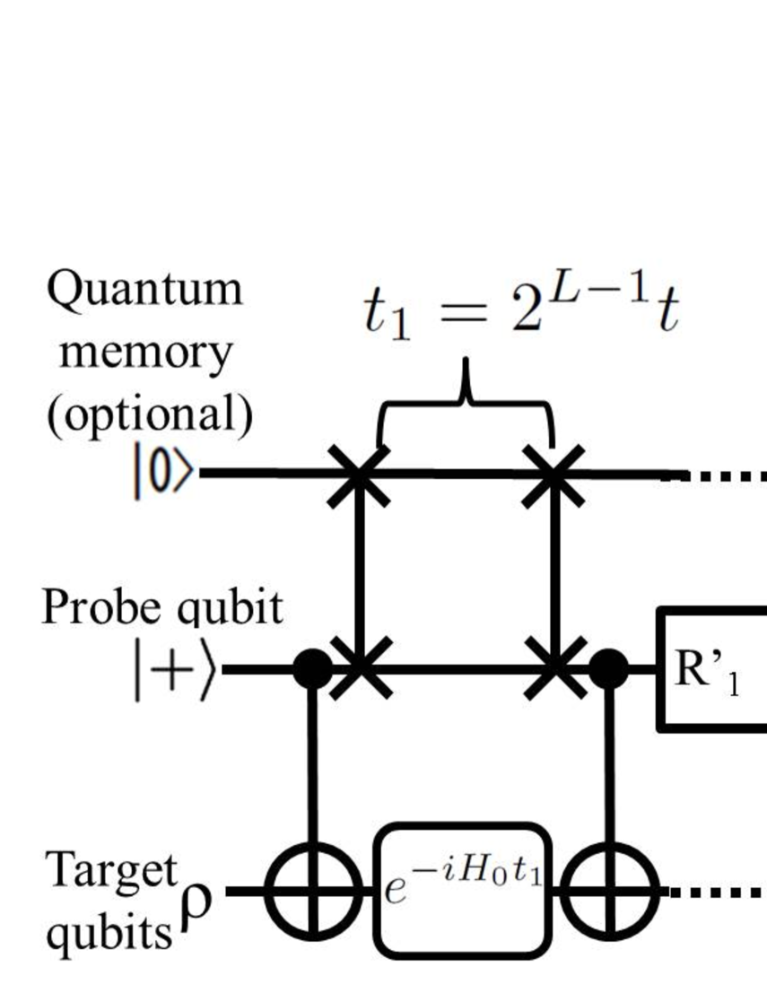
Figure 1: A quantum circuit representing our protocol for PME. A combination of the CNOT gates and free time evolution for a time $t$ provides the probe qubit with a phase information of the target systems. To avoid decoherence on the probe qubit, we perform a SWAP gate between the probe qubit and memory qubit (with a long coherence time) before and after the free evolution of the target system. To perform a Fourier basis measurement, we reset, rotate, and measure the probe qubit $L$ times where $R_{j}$ denotes the unitary rotation whose angle is defined by the previous measurement outcomes: $R_{j}^{\prime}=|1\rangle\langle 1|-\phi_{j}^{\prime}|0\rangle\langle 0|$ with $\phi^{\prime}_{j}={\rm{Exp}}[-2\pi i\sum_{k=2}^{j}m_{j-k}/2^{k}]$. The measurement outcomes reveal the energy eigenvalues of the target qubits, and induce the energy projection.

By combining the controlled unitary gate and Fourier basis measurements, the PME is implementable. A quantum circuir representing our protocol is shown in the Fig. 1. To perform the Fourier basis measurement, we recycle the single probe qubit by using the method proposed in Griffiths and Niu (1996); Parker and Plenio (2000). We measure the probe qubit $L$ times, and obtain measurement outcomes $\{m_{j}\}^{j=L}_{j=1}$. From these, eigenvalues of the target can be estimated as $\sum_{j=1}^{N}\delta\omega_{j}\cdot(s_{j}-\frac{1}{2})\simeq 2^{-L}m\frac{\pi}{t}$ where $m=\sum_{j=1}^{L}2^{L-j}m_{j-1}$, and this operation projects the target state to one of the energy eigenstates. The Kraus operator of our PME protocol on the target qubit is calculated as

$$\hat{V}_{m}=\sum_{s_{1},\cdots,s_{L}=0,1}e^{-2\pi i\frac{m}{2^{L}}\sum_{j=1}^{L}2^{L-j}s_{j}}\bigotimes_{j=1}^{N}\prod_{k=1}^{L}U_{s_{k},2^{L-k}t}^{(j)}\ \$$ (4)

where $U_{s,t}^{(j)}=e^{-iH^{(-)}_{j,|s\rangle_{\rm{P}}}\frac{\pi}{\lambda}}e^{-iH_{\rm{0}}t}e^{-iH^{(+)}_{j,|s\rangle_{\rm{P}}}\frac{\pi}{\lambda}}$. The probability to obtain the measurement outcome $m$ is $P_{m}=(\bigotimes_{j=1}^{N}{}_{T_{j}}\langle s_{j}|)\hat{V}_{m}^{\dagger}\hat{V}_{m}(\bigotimes_{j=1}^{N}|s_{j}\rangle_{T_{j}})$ and the post-measurement state of the target qubits is described as $|\psi_{m}\rangle_{T}=\frac{1}{\sqrt{P_{m}}}\hat{V}_{m}(\bigotimes_{j=1}^{N}|s_{j}\rangle_{T_{j}})$. For a quantum non-demolition measurement of energy Braginsky and Khalili (1996), an average fidelity $F=\sum_{m}P_{m}F_{m}$ should be unity where $F_{m}=|{}_{T}\langle\psi_{m}|(\bigotimes_{j=1}^{N}|s_{j}\rangle_{T_{j}})|^{2}$. We define $\epsilon=1-F$ as a projection error of the PME protocol.

We discuss possible physical systems to realize our protocol. Nitrogen vacancy (NV) centers in diamond are one of the candidates. We can control the NV center by applying microwave pulse, and also readout the spin state of the NV center by an optical detection Doherty et al. (2013). The NV center is coupled with nuclear spins via a hyperfine couplings Neumann et al. (2008); Shimo-Oka et al. (2015). We could implement our PME on the nuclear spins by using the NV center as a probe qubit. Superconducting circuits are also promising candidates. Recently, a coherent coupling between a superconducting qubit ensemble and a microwave resonator has been demonstrated Macha et al. (2014); Kakuyanagi et al. (2016), and our PME is implementable on the superconducting qubits via the microwave cavity if we control the microwave cavity as an effective two-level system by using a Kerr effect Heeres et al. (2015).

Among many candidates, we especially focus on a superconducting flux qubit coupled with an electron spin ensemble Clarke and Wilhelm (2007); Marcos et al. (2010); Twamley and Barrett (2010). Here, we could implement our PME protocol on the electron spins by using the flux qubit as a probe. High fidelity control and readout of the superconducting flux qubit have been demonstrated Clarke and Wilhelm (2007). Recently, a coherent coupling between the flux qubit and the electron spin ensemble was observed, and the coupling strength between a single electron spin and a flux qubit is estimated as $g/2\pi=10$ kHz Zhu et al. (2011). Moreover, there is a theoretical proposal to increase coupling up to $g/2\pi=100$ kHz Twamley and Barrett (2010). Although the coherence time of the flux qubit is still around 80 micro seconds Yan et al. (2015) which may not be long enough to realize the PME protocol, a quantum memory for the superconducting qubit with much longer coherence time such as microwave cavitys and solid state spin systems can be used Marcos et al. (2010); Twamley and Barrett (2010); Tyryshkin et al. (2012); Reagor et al. (2015). Especially, if we can use the nuclear spins for the quantum memory of the flux qubit, the coherence time can be an order of an hour Saeedi et al. (2013). In this letter, we especially consider these systems.

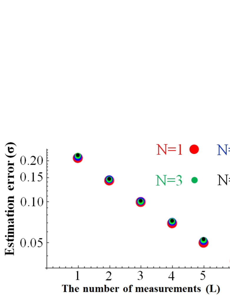
Figure 2: The variance ($\sigma$) of estimation against the number of measurements ($L$). The parameters are $g/2\pi=100$ kHz, $t\sqrt{N}=0.16$ ms, and $\sigma_{\rm{G}}/2\pi=1$kHz where $N$ denotes the number of the target qubits. In our scheme, $\sigma$ decreases exponentially with $L$.

We investigate the performance of the PME protocol where a single target qubit is coupled with a probe qubit. We assume that the initial state of the target qubit is $|0\rangle_{\rm{T}_{1}}$ where the detuning of the target qubit $\delta\omega_{1}$ has a Gaussian distribution with a zero average and a variance of $\sigma_{\rm{G}}$. The performance of our PME protocol depends on the value of $\delta\omega_{1}$. To evaluate the average performance of our protocol, we randomly pick up $N_{\rm{r}}$ values of the detuning $\{\delta\omega^{(l)}_{1}\}^{l=N_{\rm{r}}}_{l=1}$ from the Gaussian distribution, and we will take an average.

We numerically calculate the variance of the estimated energy eigenvalues in our protocol. The variance is defined as

$$\sigma = \frac{1}{N_{\rm{r}}}\sum_{l=1}^{N_{r}}\sqrt{\sum_{m=0}^{2^{L-1}}P^{(l)}_{m}(f_{m}-\frac{\delta\omega^{(l)}_{1}t}{2\pi})^{2}}$$ (5)

where $P^{(l)}_{m}$ denotes a probability to obtain a measurement outcome of $m$ for a given $\delta\omega^{(l)}_{1}$. The function $f_{m}=(2^{-L}m-1)\cdot H_{2^{-L}m-0.5}+2^{-L}m(1-H_{2^{-L}m-0.5})$ plays a role to remove the ambiguity due to the phase periodicity where $H_{x}$ denotes a Heaviside step function. We plot the variance by the simulations in Fig. 2. The variance decreases exponentially with the number of measurements $\sigma\propto 2^{-\frac{L}{2}}$, which is consistent with the scaling of the typical QPE protocol Higgins et al. (2007); Berry et al. (2009).

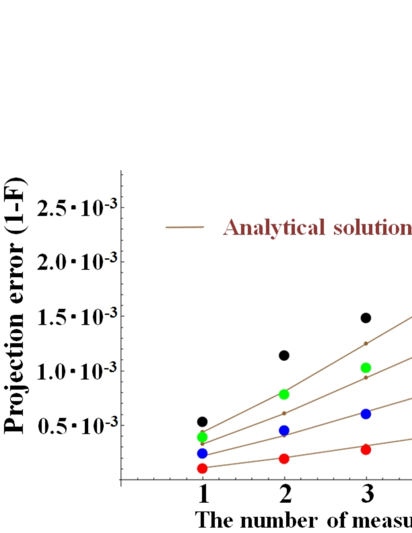
Figure 3: The projection errors $(1-F)$ against the number of measurements $(L)$ where $F$ denotes a fidelity of the post measurement states. The projection error increases linearly with the number of the target qubits $N$. We use the same parameters as in the Fig. 2.

We calculate the average fidelity between the initial state and the post-measurement state of the single target qubit. We define the fidelity as $F=\frac{1}{N_{\rm{r}}}\sum_{l=1}^{N_{r}}\sum_{m=0}^{2^{L-1}}P^{(l)}_{m}F^{(l)}_{m}$ where $P^{(l)}_{m}$ ($F_{m}^{(l)}$ ) denote the probability (fidelity) for a measurement outcome of $m$ for a given $\delta\omega^{(l)}_{1}$. If the fidelity is close to the unity, we obtain an analytical solution of the projection error

$$\epsilon\simeq\sum_{n=0}^{L-1}\frac{3(64+3\pi^{2}+e^{-\frac{1}{2}\sigma^{2}_{\rm{G}}(2^{n}t)^{2}}(64-3\pi^{2})(1-\sigma^{2}_{\rm{G}}(2^{n}t)^{2}))}{256(\frac{g}{\sigma_{\rm{G}}})^{2}}$$

We plot the projection error of both numerical simulations and analytical results in Fig. 3. This analytical solutions agree with the numerical simulations.

We calculate the estimate variance of our PME for multiple target qubits. Without loss of generality, we can assume the initial state of the target qubits is $\bigotimes_{j=1}^{N}|0\rangle_{\rm{T}_{j}}$. We define the variance for multiple target qubits by Eq. 5 where we replace $\delta\omega_{1}^{(l)}$ with $\delta\omega_{l}=\sum_{j=1}^{N}\delta\omega^{(l)}_{j}$. Here, $\delta\omega^{(l)}_{j}$ denotes a detuning at the $j$ th target qubit where we randomly pick up $N_{\rm{r}}$ values of the detuning $\{\delta\omega^{(l)}_{j}\}^{l=N_{\rm{r}}}_{l=1}$ from a Gaussian distribution with zero average and variance of $\sigma_{\rm{G}}$. Since we have $\delta\omega t=\frac{1}{N_{\rm{r}}}\sum_{l=1}^{N_{\rm{r}}}\delta\omega_{l}\simeq\sqrt{N}\sigma_{\rm{G}}t$ from the central limit theorem, we obtain $\delta\omega t=\Theta(N^{0})$ by choosing $t=\Theta(N^{-\frac{1}{2}})$. So we can remove the $N$ dependency of the variance. We confirm this from numerical simulations, and plot the results in Fig. 2. Similar to the single target qubit case, we can exponentially suppress the estimation variance for multiple target qubits as we increase the number of the measurements.

We also calculate the projection error for multiple target qubits. For a single target qubit, we obtained an analytical solution of the projection error $\epsilon$. For a small projection error, the total projection error for $N$ target qubits will be approximated as $N\epsilon$. We plot the analytical solution and numerical results in the Fig. 3, and there is a good agreement between the analytical and numerical results. Since the projection error is proportional to the number of the target qubits, our PME works efficiently for a relatively small number of target qubits. For example, from the simulation, the projection error is estimated around $0.27\%$ for $N=4$ and $L=6$ with the current parameters. To decrease the projection error for a larger number of the target qubits, we should increase the coupling strength between the probe and target qubits, which would be possible by changing the design of the qubits Twamley and Barrett (2010); Yoshihara et al. (2016).

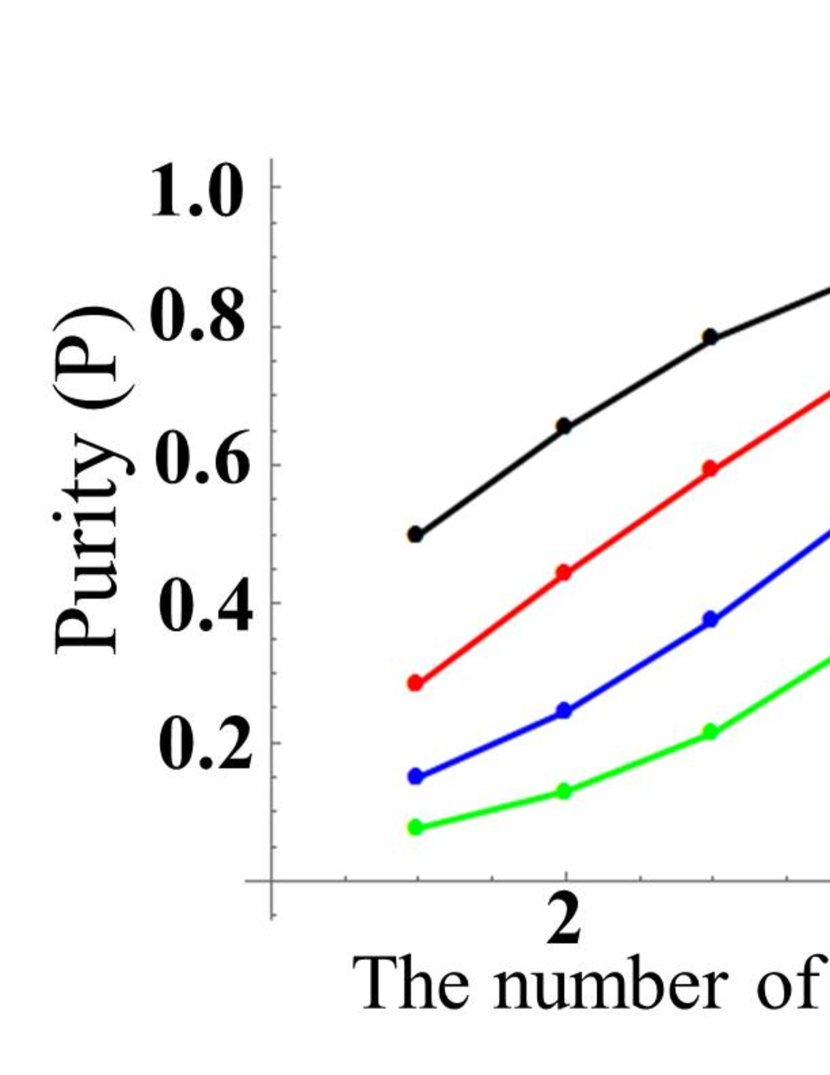
Figure 4: The purity of the state against the number of measurements. We use the same parameters as in the Fig. 2. The purity approaches to the unity as we increase the number of the measurements. Each continuous line is a guide for the eyes.

Finally, we calculate the purity of the post-measurement state when the initial state is a completely mixed state. For a given set of the detuning $\delta\omega_{j}^{(l)}$ $(j=1,2,\cdots,N)$, the post-measurement state is calculated as $\rho^{(l)}_{m}=\frac{\hat{V}^{(l)}_{m}\frac{1}{2^{N}}\hat{\openone}(\hat{V}^{(l)}_{m})^{\dagger}}{{\rm{Tr}}[\hat{V}_{m}\frac{1}{2^{N}}\hat{\openone}(\hat{V}^{(l)}_{m})^{\dagger}]}$. The average purity is calculated as $P=\frac{1}{N_{\rm{r}}}\sum_{l=1}^{N_{\rm{r}}}(\rho^{(l)}_{m})^{2}$. We plot this results in Fig. 4. As we increase the number of the measurements, the purity approaches to the unity.

In conclusion, we propose a protocol to implement the projective measurement of energy on an ensemble of qubits with unknown frequencies. We use a quantum phase estimation algorithm to determine the unknown energy of the target system. Unlike previous protocols, we only require a single probe qubit and global operations for the implementation, which makes it more feasible to realize. Our scheme has many potential applications such as characterization of unknown quantum systems, quantum metrology, and initialization.

This work was supported by JSPS KAKENHI Grant 15K17732, and was also partially supported by MEXT KAKENHI Grant Number 15H05870, 16H01050, and 24106009.

References

- von Neumann (1932) J. von Neumann, Mathematische Grundlagen der Quantenmechanik (Springer, 1932).
- Koshino and Shimizu (2005) K. Koshino and A. Shimizu, Phys. Rep. 412, 191 (2005).
- Wiseman and Milburn (2009) H. M. Wiseman and G. J. Milburn, Quantum measurement and control (Cambridge University Press, 2009).
- Aharonov et al. (2002) Y. Aharonov, S. Massar, and S. Popescu, Phys. Rev. A 66, 052107 (2002).
- Chuang and Nielsen (1997) I. L. Chuang and M. A. Nielsen, Journal of Modern Optics 44, 2455 (1997).
- Poyatos et al. (1997) J. Poyatos, J. I. Cirac, and P. Zoller, Phys. Rev. Lett. 78, 390 (1997).
- Nakayama et al. (2015) S. Nakayama, A. Soeda, and M. Murao, Phys. Rev. Lett. 114, 190501 (2015).
- Kitaev et al. (2002) A. Y. Kitaev, A. Shen, and M. N. Vyalyi, Classical and quantum computation, vol. 47 (American Mathematical Society Providence, 2002).
- Griffiths and Niu (1996) R. B. Griffiths and C.-S. Niu, Phys. Rev. Lett. 76, 3228 (1996).
- Parker and Plenio (2000) S. Parker and M. B. Plenio, Phys. Rev. Lett. 85, 3049 (2000).
- Braginsky and Khalili (1996) V. B. Braginsky and F. Y. Khalili, Reviews of Modern Physics 68, 1 (1996).
- Doherty et al. (2013) M. W. Doherty, N. B. Manson, P. Delaney, F. Jelezko, J. Wrachtrup, and L. C. Hollenberg, Physics Reports 528, 1 (2013).
- Neumann et al. (2008) P. Neumann, N. Mizuochi, F. Rempp, P. Hemmer, H. Watanabe, S. Yamasaki, V. Jacques, T. Gaebel, F. Jelezko, and J. Wrachtrup, Science 320, 1326 (2008).
- Shimo-Oka et al. (2015) T. Shimo-Oka, H. Kato, S. Yamasaki, F. Jelezko, S. Miwa, Y. Suzuki, and N. Mizuochi, Appl. Phys. Lett. 106, 153103 (2015).
- Macha et al. (2014) P. Macha, G. Oelsner, J. M. Reiner, M. Marthaler, S. André, G. Schön, U. Hübner, H. G. Meyer, E. llIichev, and A. V. Ustinov, Nature communications 5 (2014).
- Kakuyanagi et al. (2016) K. Kakuyanagi, Y. Matsuzaki, C. Deprez, H. Toida, K. Semba, H. Yamaguchi, W. J. Munro, and S. Saito, arXiv preprint arXiv:1606.04222 (2016).
- Heeres et al. (2015) R. W. Heeres, B. Vlastakis, E. Holland, S. Krastanov, V. V. Albert, L. Frunzio, L. Jiang, and R. J. Schoelkopf, Phys. Rev. Lett. 115, 137002 (2015).
- Clarke and Wilhelm (2007) J. Clarke and F. K. Wilhelm, Nature 453, 1031 (2007).
- Marcos et al. (2010) D. Marcos, M. Wubs, J. M. Taylor, R. Aguado, M. D. Lukin, and A. S. Sørensen, Phys. Rev. Lett. 105, 210501 (2010).
- Twamley and Barrett (2010) J. Twamley and S. D. Barrett, Phys. Rev. B 81, 241202 (2010).
- Zhu et al. (2011) X. Zhu, S. Saito, A. Kemp, K. Kakuyanagi, S. Karimoto, H. Nakano, W. J. Munro, Y. Tokura, M. S. Everitt, K. Nemoto, et al., Nature 478, 221 (2011).
- Yan et al. (2015) F. Yan, S. Gustavsson, A. Kamal, J. Birenbaum, A. Sears, D. Hover, T. Gudmundsen, J. Yoder, T. Orlando, J. Clarke, et al., arXiv preprint arXiv:1508.06299 (2015).
- Tyryshkin et al. (2012) A. M. Tyryshkin, S. Tojo, J. J. Morton, H. Riemann, N. V. Abrosimov, P. Becker, H.-J. Pohl, T. Schenkel, M. L. Thewalt, K. M. Itoh, et al., Nature materials 11, 143 (2012).
- Reagor et al. (2015) M. Reagor, W. Pfaff, C. Axline, R. W. Heeres, N. Ofek, K. Sliwa, E. Holland, C. Wang, J. Blumoff, K. Chou, et al., arXiv preprint arXiv:1508.05882 (2015).
- Saeedi et al. (2013) K. Saeedi, S. Simmons, J. Z. Salvail, P. Dluhy, H. Riemann, N. V. Abrosimov, P. Becker, H.-J. Pohl, J. J. Morton, and M. L. Thewalt, Science 342, 830 (2013).
- Higgins et al. (2007) B. L. Higgins, D. W. Berry, S. D. Bartlett, H. M. Wiseman, and G. J. Pryde, Nature 450, 393 (2007).
- Berry et al. (2009) D. W. Berry, B. L. Higgins, S. D. Bartlett, M. W. Mitchell, G. J. Pryde, and H. M. Wiseman, Phys. Rev. A 80, 052114 (2009).
- Yoshihara et al. (2016) F. Yoshihara, T. Fuse, S. Ashhab, K. Kakuyanagi, S. Saito, and K. Semba, arXiv preprint arXiv:1602.00415 (2016).