Riemannian Tensor Completion
with Side Information

Tengfei ZhouHui QianZebang ShenCongfu Xu
Computer Science Institute, Zhejiang University
{zhoutengfei_zju, qianhui, shenzebang, xucongfu@zju.edu.cn}
Corresponding author.
Abstract

By restricting the iterate on a nonlinear manifold, the recently proposed Riemannian optimization methods prove to be both efficient and effective in low rank tensor completion problems. However, existing methods fail to exploit the easily accessible side information, due to their format mismatch. Consequently, there is still room for improvement in such methods. To fill the gap, in this paper, a novel Riemannian model is proposed to organically integrate the original model and the side information by overcoming their inconsistency. For this particular model, an efficient Riemannian conjugate gradient descent solver is devised based on a new metric that captures the curvature of the objective. Numerical experiments suggest that our solver is more accurate than the state-of-the-art without compromising the efficiency.

I.   Introduction

Low Rank Tensor Completion (LRTC) problem, which aims to recover a tensor from its linear measurements, arises naturally in many artificial intelligence applications. In hyperspectral image inpainting, LRTC is applied to interpolate the unknown pixels based on the partial observation   Xu et al. (2015). In recommendation tasks, LRTC helps users find interesting items under specific contexts such as locations or time  Liu et al. (2015). In computational phenotyping, one adopts LRTC to discovery phenotypes in heterogeneous electronic health records  Wang et al. (2015).

Euclidean Models: LRTC can be formulated by a variety of optimization models over the Euclidean space. Amongst them, convex models that encapsulate LRTC as a regression problem penalized by a tensor nuclear norm are the most popular and well-understood  Romera-Paredes and Pontil (2013), Zhang et al. (2014). Though most of them have sound theoretical guarantees  Zhang and Aeron (2016), Chen et al. (2013), Yuan and Zhang (2015), in general, their solvers are ill-suited for large tensors because these procedures usually involve Singular Value Decomposition (SVD) of huge matrices per iteration  Liu et al. (2013). Another class of Euclidean models is formulated as the decomposition problem that factorizes a low rank tensor into small factors  Jain and Oh (2014), Filipović and Jukić (2015), Xu et al. (2015). Many solvers for such decomposition based model have been proposed to recover large tensors, and low per-iteration computational cost is illustrated  Beutel et al. (2014), Liu et al. (2014), Smith et al. (2016).

Riemannian Models: LRTC can also be modeled by nonconvex optimization constrained on Riemannian manifolds   Kressner et al. (2014), Kasai and Mishra (2016), which is easily handled by many manifold based solvers  Absil et al. (2009). Empirical comparison has shown that Riemannian solvers use significantly less CPU time to recover the underlying tensor in contrast to the Euclidean solvers  Kasai and Mishra (2016). The main reason resides in that such solvers avoid SVD of huge matrices by explicitly exploiting the geometrical structure of LRTC, which makes them more suitable for massive problem.

Of all the Riemanian models, two search spaces, fix multi-linear rank manifold  Kressner et al. (2014) and Tucker manifold  Kasai and Mishra (2016), are usually employed. The former is a sub-manifold of Euclidean space, and the latter is a quotient manifold induced by the Tucker decomposition. Generally, quotient manifold based solvers have higher convergence rates because it is usually easier to design a pre-conditioner for them  Kasai and Mishra (2016), Mishra and Sepulchre (2016).

Side Information: In the Euclidean models of LRTC, side information is helpful in improving the accuracy   Narita et al. (2011), Acar et al. (2011), Beutel et al. (2014). One common form of the side information is the feature matrix, which measures the statistical properties of tensor modes  Kolda and Bader (2009). For example, in Netflix tasks, feature matrix can be built from the demography of users  Bell and Koren (2007). Another form is the similarity matrix, which quantifies the resemblance between two entities of a tensor mode. For instance, the social network generates the similarity matrix by utilizing the correspondence between users  Rai et al. (2015). In practice, these two matrices can be transformed to each other, and we only consider the feature matrix case throughout this paper.

However, as far as we know, side information has not been incorporated in any Riemannian model. The first difficulty lies in the model design. Fusing the side information into the Riemannian model inevitably compromises the integrity of the low rank tensor due to the compactness of the manifold. The second difficulty results from the solver design. Incorporating the side information may aggravate the ill-conditioning of LRTC problem and degenerates the convergence significantly.

Contributions: To address these difficulties, a novel Riemannian LRTC method is proposed from the perspective of both model and solver designs. By exploring the relation between the subspace spanned by the tensor fibers and the column space of the feature matrix, we explicitly integrate the side information in a compact way. Meanwhile, a first order solver is devised under the manifold optimization framework. To ease the ill-conditioning, we design a novel metric based on an approximated Hessian of the cost function. The metric implicitly induce an adaptive preconditioner for our solver. Empirical studies illustrate that our method achieves much more accurate solutions within comparable processing time than the state-of-the-art.

II.   Notations and Preliminaries

In this paper, we only focus on the $3$rd order tensor, but generalizing our method to high order is straight forward. We use the notation $\mathbf{X}\in\mathbb{R}^{n\times m}$ to denote a matrix, and the notation $\mathbfcal{X}\in\mathbb{R}^{n_{1}\times\cdots\times n_{d}}$ to denote a $d$-th order tensor. We also denote by $\mathbfcal{X}(i_{1},\cdots,i_{d})$ the element in position $(i_{1},\cdots,i_{d})$ of $\mathbfcal{X}$. For many cases, we use curly braces with indexes to simplify the notation. For example, $\{\mathbf{O}_{i}\}_{i=1}^{3}$ is used to denote $\mathbf{O}_{1},\mathbf{O}_{2},\mathbf{O}_{3}$, and $\{\mathbf{U}_{i}\mathbf{O}_{i}\}_{i=1}^{3}$ refer to $\mathbf{U}_{1}\mathbf{O}_{1},\mathbf{U}_{2}\mathbf{O}_{2},\mathbf{U}_{3}\mathbf{O}_{3}$.

Mode-$k$ Fiber and matricization: A fiber of a tensor is obtained by varying one index while fixing the others, i.e. $\mathbfcal{X}(i_{1},\cdots,i_{k-1},:,i_{k+1},\cdots,i_{d})$ is the mode-$k$ fiber of a $d$-th order tensor $\mathbfcal{X}$. Here we use the colon to denote $\{1,\ldots,n_{k}\}$. A mode-$k$ matricization $\mathbfcal{X}_{(k)}\in\mathbb{R}^{n_{k}\times(n_{1}\cdots n_{k-1}n_{k+1}\cdots n_{d})}$ of a tensor $\mathbfcal{X}$ is obtained by arranging the mode-$n$ fibers of $\mathbfcal{X}$ so that each of them is a column of $\mathbfcal{X}_{(k)}$  Kolda and Bader (2009) The mode-$k$ product of tensor $\mathbfcal{X}$ and matrix $\mathbf{A}$ is denoted by $\mathbfcal{X}\times_{k}\mathbf{A}$, whose mode-$k$ matricization can be expressed as (𝒳×𝒜𝒜𝒳(\mathbfcal{X}\times_{k}\mathbf{A})_{(k)}=\mathbf{A}\mathbfcal{X}_{(k)}. For $3$rd order tensor $\mathbfcal{X}$ and matrix $\mathbf{A}_{1},\mathbf{A}_{2},\mathbf{A}_{3}$, we use 𝒳×𝒜superscriptsubscript𝒳subscript𝒜\mathbfcal{X}\times_{i=1}^{3}\mathbf{A}_{i} to denote $\mathbfcal{X}\times_{1}\mathbf{A}_{1}\times_{2}\mathbf{A}_{2}\times_{3}\mathbf{A}_{3}$.

Inner product and norm: The inner product of two tensors with the same size is defined by 𝒳𝒴𝒳𝒴delimited-⟨⟩𝒳𝒴subscriptsubscriptsubscript𝒳subscriptsubscript𝒴subscriptsubscript\langle\mathbfcal{X},\mathbfcal{Y}\rangle=\sum_{i_{1},\cdots,i_{d}}\mathbfcal{X}(i_{1},\cdots,i_{d})\mathbfcal{Y}(i_{1},\cdots,i_{d}). The Frobenius norm of a tensor $\mathbfcal{X}$ is defined by 𝒳𝒳𝒳subscriptnorm𝒳delimited-⟨⟩𝒳𝒳\|\mathbfcal{X}\|_{F}=\sqrt{\langle\mathbfcal{X},\mathbfcal{X}\rangle}.

Multi-linear rank and Tucker decomposition:  The multi-linear rank $\mathop{\rm rank^{vec}}(\mathbfcal{X})$ of a tensor $\mathbfcal{X}\in\mathbb{R}^{n_{1}\times n_{2}\times n_{3}}$ is defined as a vector $(\mathop{\rm rank}({\mathbfcal{X}_{(1)}}),\mathop{\rm rank}({\mathbfcal{X}_{(2)}}),\mathop{\rm rank}({\mathbfcal{X}_{(3)}}))$. If rankvec(𝒳\mathop{\rm rank^{vec}}(\mathbfcal{X})=(r_{1},r_{2},r_{3}), tucker decomposition factorizes $\mathbfcal{X}$ into a small core tensor ${\mathbfcal{G}}\in\mathbb{R}^{r_{1}\times r_{2}\times r_{3}}$ and three matrices $\mathbf{U}_{i}\in\mathbb{R}^{n_{i}\times r_{i}}$ with orthogonal columns, that is 𝒳𝒢×𝒰superscriptsubscript𝒳𝒢subscript𝒰\mathbfcal{X}={\mathbfcal{G}}\times_{i=1}^{3}\mathbf{U}_{i}. Note that, the tucker decomposition of a tensor is not unique. In fact, if 𝒳𝒢×𝒰superscriptsubscript𝒳𝒢subscript𝒰\mathbfcal{X}={\mathbfcal{G}}\times_{i=1}^{3}\mathbf{U}_{i}, we can easily obtain 𝒳×𝒱superscriptsubscript𝒳subscript𝒱\mathbfcal{X}={\mathbfcal{H}}\times_{i=1}^{3}\mathbf{V}_{i}, with ${\mathbfcal{H}}={\mathbfcal{G}}\times_{i=1}^{3}\mathbf{O}^{\top}_{i}$, $\mathbf{V}_{i}=\mathbf{U}_{i}\mathbf{O}_{i}$, where $\mathbf{O}_{i}\in\mathbb{R}^{r_{i}\times r_{i}}$ is any orthogonal matrix. Thus, we obtain the equivalent class

$$[{\mathbfcal{G}},\{\mathbf{U}_{i}\}_{i=1}^{3}]\triangleq\{({\mathbfcal{G}}\times_{i=1}^{3}\mathbf{O}_{i}^{\top},\{\mathbf{U}_{i}\mathbf{O}_{i}\}_{i=1}^{3})|\mathbf{O}_{i}^{\top}\mathbf{O}_{i}=\mathbf{I}_{i}\}.$$

For simplicity, we denote $[{\mathbfcal{G}},\{\mathbf{U}_{i}\}_{i=1}^{3}]$ by $[\mathbfcal{X}]$, when 𝒳𝒢×𝒰superscriptsubscript𝒳𝒢subscript𝒰\mathbfcal{X}={\mathbfcal{G}}\times_{i=1}^{3}\mathbf{U}_{i}. Usually, $[\mathbfcal{X}]$ is called the Tucker representation of $\mathbfcal{X}$, while $\mathbfcal{X}$ is call the tensor representation of $[\mathbfcal{X}]$. We also use $\overline{\mathbfcal{X}}$ to denote a specific decomposition of $\mathbfcal{X}$, additionally $\overline{\mathbfcal{X}}\in[\mathbfcal{X}]$.

II.1 Search Space of Riemannian Models

The Tucker manifold that we used in our Riemannian model is a quotient manifold induced by the Tucker decomposition. In order to lay the ground for Tucker manifold, we first describe its counterpart, the fix multi-rank manifold, which will be helpful in understanding the whole derivation.

A fixed multi-linear rank manifold $\mathcal{F}_{r}$ consists of tensors with the same fixed multi-linear rank. Specifically

r={𝒳\×\×\\𝒳}subscript𝑟𝒳superscriptsubscript\subscript\subscript\\superscript𝒳\mathcal{F}_{r}=\{\mathbfcal{X}\in\mathbb{R}^{n_{1}\times n_{2}\times n_{3}}|\mathop{\rm rank^{vec}}(\mathbfcal{X})=r\}.

To define the Tucker manifold, we first define a total space

$${\mathcal{M}_{r}}=\mathbb{R}^{r_{1}\times r_{2}\times r_{3}}\times\mathop{\rm St}(r_{1},n_{1})\times\mathop{\rm St}(r_{2},n_{2})\times\mathop{\rm St}(r_{3},n_{3}),$$ (1)

in which $\mathop{\rm St}(r_{i},n_{i})$ is the Stiefel manifold of a $n_{i}\times r_{i}$ matrix with orthogonal columns. Then, we can depict the Tucker manifold of multi-linear rank $r$ as follows.

$${\mathcal{M}_{r}}/\sim\triangleq\left\{[{\mathbfcal{G}},\{\mathbf{U}_{i}\}_{i=1}^{3}]|({\mathbfcal{G}},\{\mathbf{U}_{i}\}_{i=1}^{3})\in{\mathcal{M}_{r}}\right\}.$$ (2)

The Tucker manifold is a quotient manifold of the total space (1). We use the abstract quotient manifold, rather than the concrete total space, as search space because the non-uniqueness of the Tucker decomposition is undesirable for optimization. Note that such non-uniqueness will introduce more local optima into the minimization. The relation of manifold $\mathcal{F}_{r}$ and ${\mathcal{M}_{r}}/\sim$ is characterized as follows.

Proposition 1.

The quotient manifold ${\mathcal{M}_{r}}/\sim$ is diffeomorphic to the fix multi-linear rank manifold $\mathcal{F}_{r}$, with diffeomorphism $\rho(\cdot)$ from $\mathcal{F}_{r}$ to ${\mathcal{M}_{r}}/\sim$ defined by ρ(𝒳𝒢{𝒰}\rho(\mathbfcal{X})=[{\mathbfcal{G}},\{\mathbf{U}_{i}\}_{i=1}^{3}] where $[{\mathbfcal{G}},\{\mathbf{U}_{i}\}_{i=1}^{3}]$ is the tucker representation of $\mathbfcal{X}$.

This proposition says that each tensor $\mathbfcal{X}\in\mathcal{F}_{r}$ can be represented by a unique equivalent class $[{\mathbfcal{G}},\{\mathbf{U}_{i}\}_{i=1}^{3}]\in\mathcal{M}/\sim$ and vice-versa.

II.2 Vanilla Riemannian Tensor Completion

The purest incarnation of Riemannian tensor completion model is the Riemannian model over the fix multi-linear rank manifold. Let ${\mathbfcal{R}}\in\mathbb{R}^{n_{1}\times n_{2}\times n_{3}}$ be a partially observed tensor. Let $\Omega$ be the set which contains the indices of observed entries. The model can be expressed as:

$$\min_{\mathbfcal{X}}\frac{1}{2}\|{\mathbf{\mathcal{P}}_{\Omega}}(\mathbfcal{X}-{\mathbfcal{R}})\|_{F}^{2}\quad{\text{s.b.t}}\quad\mathbfcal{X}\in\mathcal{F}_{r},$$ (3)

with ${\mathbf{\mathcal{P}}_{\Omega}}$ maps $\mathbfcal{X}$ to the sparsified tensor ${\mathbf{\mathcal{P}}_{\Omega}}(\mathbfcal{X})$, where 𝒫Ω(𝒳𝒳{\mathbf{\mathcal{P}}_{\Omega}}(\mathbfcal{X})(i_{1},i_{2},i_{3})=\mathbfcal{X}(i_{1},i_{2},i_{3}) if $(i_{1},i_{2},i_{3})\in\Omega$, and 𝒫Ω(𝒳{\mathbf{\mathcal{P}}_{\Omega}}(\mathbfcal{X})(i_{1},i_{2},i_{3})=0 otherwise.

Another popular model, Tucker model, is based on the quotient manifold ${\mathcal{M}_{r}}/\sim$, which can be expressed as:

$$\min_{\mathbfcal{X}}\frac{1}{2}\|{\mathbf{\mathcal{P}}_{\Omega}}(\rho^{-1}([\mathbfcal{X}])-{\mathbfcal{R}})\|_{F}^{2}\quad{\text{s.b.t}}\quad[\mathbfcal{X}]\in{\mathcal{M}_{r}}/\sim,$$ (4)

with $\rho$ defined in Prop. 1.

Note that since the dawn of Riemannian framework for LRTC, a quandary exists: on one hand, sparse measurement limits the capacity of the solution; on the other hand, rich side information can not be incorporated into this framework. In many artificial intelligence applications, demands for high accuracy further exacerbates such dilemma.

III.   Riemannian Model with Side Information

We focus on the case that the side information is encoded in feature matrices $\mathbf{P}_{i}\in\mathbb{R}^{n_{i}\times k_{i}}$. Suppose ${\mathbfcal{R}}\in\mathcal{F}_{r}$ has tucker factors $({\mathbfcal{G}},\{\mathbf{U}_{i}\}_{i=1}^{3})$.Without loss of generality, we assume that $k_{i}\geq r_{i}$ and $\mathbf{P}_{i}$ has orthogonal columns.

In the ideal case, we assume that

$$\mathop{\rm span}(\mathbf{U}_{i})\subset\mathop{\rm span}(\mathbf{P}_{i}).$$ (5)

Such relation means that the feature matrices contain all the information in the latent space of the underlying tensor. Equivalently, there exists a matrix $\mathbf{W}_{i}$ such that $\mathbf{U}_{i}=\mathbf{P}_{i}\mathbf{W}_{i}$. However, in practice, due to the existence of noise, one can only expect such relation to hold approximately, i.e. $\mathbf{U}_{i}\approx\mathbf{P}_{i}\mathbf{W}_{i}$. Incorporating such relation to a tensor completion model via penalization, we have the following formulation

$\displaystyle\min_{{\mathbfcal{G}},\mathbf{U}_{i},\mathbf{W}_{i}}L({\mathbfcal{G}},\{\mathbf{U}\}_{i=1}^{3})+\sum_{i=1}^{3}\frac{\alpha_{i}|\Omega|}{2}\|\mathbf{U}_{i}-\mathbf{P}_{i}\mathbf{W}_{i}\|_{F}^{2},$ (6)
$\displaystyle\quad\text{s.t.}\quad({\mathbfcal{G}},\{\mathbf{U}_{i}\}_{i=1}^{3})\in{\mathcal{M}_{r}},$

where $L({\mathbfcal{G}},\{\mathbf{U}_{i}\}_{i=1}^{3})=\|{\mathbf{\mathcal{P}}_{\Omega}}({\mathbfcal{G}}\times_{i=1}^{3}\mathbf{U}_{i}-{\mathbfcal{R}})\|_{F}^{2}/2$. Fixing ${\mathbfcal{G}}$ and $\mathbf{U}_{i}$, with respect to $\mathbf{W}_{i}$, (6) has a close form solution

$$\mathbf{W}_{i}=(\mathbf{P}_{i}^{\top}\mathbf{P}_{i})^{-1}\mathbf{P}_{i}^{\top}\mathbf{U}_{i}=\mathbf{P}_{i}^{\top}\mathbf{U}_{i}.$$ (7)

Since $\min_{x,y}l(x,y)=\min_{x}l(x,y(x))$ where $y(x)=\arg\min_{y}l(x,y)$, one can substitute (7) into the above problem and obtain the following equivalence

$\displaystyle\min_{{\mathbfcal{G}},\mathbf{U}_{i}}L({\mathbfcal{G}},\{\mathbf{U}\}_{i=1}^{3})+\sum_{i=1}^{3}\frac{\alpha_{i}|\Omega|}{2}\mathop{\rm trace}(\mathbf{U}_{i}^{T}(\mathbf{I}_{i}-\mathbf{P}_{i}\mathbf{P}_{i}^{T})\mathbf{U}_{i})$ (8)
$\displaystyle\quad\triangleq f({\mathbfcal{G}},\{\mathbf{U}_{i}\}_{i=1}^{3})$
$\displaystyle\quad\text{s.t.}\quad({\mathbfcal{G}},\{\mathbf{U}_{i}\}_{i=1}^{3})\in{\mathcal{M}_{r}}.$

Although the cost function is already smooth over the total space ${\mathcal{M}_{r}}$, due to its invariance over the equivalent class $[{\mathbfcal{G}},\{\mathbf{U}_{i}\}_{i=1}^{3}]$, there can be infinite local optima, which is extremely undesirable. Indeed, if $({\mathbfcal{G}},\{\mathbf{U}_{i}\}_{i=1}^{3})$ is a local optimal of the objective, then so is every point in the infinite set $[{\mathbfcal{G}},\{\mathbf{U}_{i}\}_{i=1}^{3}]$. One way to reduce the number of local optima is to mathematically treated the entire set $[{\mathbfcal{G}},\{\mathbf{U}_{i}\}_{i=1}^{3}]$ as a point. Consequently, we redefine the cost by $\tilde{f}([{\mathbfcal{G}},\{\mathbf{U}_{i}\}_{i=1}^{3}])=f({\mathbfcal{G}},\{\mathbf{U}_{i}\}_{i=1}^{3})$ and obtain the following Remainnian optimization problem over the quotient manifold ${\mathcal{M}_{r}}/\sim$:

$$\min_{[\mathbfcal{X}]}\tilde{f}([\mathbfcal{X}])\quad\text{s.t.}\quad[\mathbfcal{X}]\in{\mathcal{M}_{r}}/\sim.$$ (9)
Remark 1.

In Riemannian optimization literature, problem (8) is called the lifted representation of problem (9) over the total space Absil et al. (2009). This model is closely related to the Laplace regularization model Narita et al. (2011). Concretely, they share the same form:

$$\min_{{\mathbfcal{G}},\mathbf{U}_{i}}L({\mathbfcal{G}},\{\mathbf{U}_{i}\}_{i=1}^{3})+\sum_{i=1}^{3}\frac{C_{i}}{2}\mathop{\rm trace}(\mathbf{U}_{i}^{\top}\mathbf{L}_{i}\mathbf{U}_{i}).$$ (10)

The difference lies in that $\mathbf{L}_{i}$ is a projection matrix in our case, while, in the Laplace regularization model, $\mathbf{L}_{i}$ is a Laplacian matrix.

Remark 2.

Since each $[\mathbfcal{X}]\in\mathcal{M}_{r}/\sim$ has a unique tensor representation in $\mathbfcal{X}\in\mathcal{F}_{r}$, we show that the abstract model (9) can be represented as a concrete model over the manifold $\mathcal{F}_{r}$. Specifically, the following Proposition interprets the proposed model as an optimization problem with a regularizer that encourages the mode-$i$ space of the estimated tensor close to $\mathop{\rm span}(\mathbf{P}_{i})$.

Proposition 2.

if $[\mathbfcal{X}]$ is a critical point of problem (9) then its tensor representation $\mathbfcal{X}$ is a critical point of the following problem.

min𝒳12𝒫Ω(𝒳αΩ\𝒳\𝒫\displaystyle\min_{\mathbfcal{X}\in\mathcal{F}_{r}}\frac{1}{2}\|{\mathbf{\mathcal{P}}_{\Omega}}(\mathbfcal{X}\!-\!{\mathbfcal{R}})\|_{F}^{2}\!+\!\sum_{i=1}^{3}\frac{\alpha_{i}|\Omega|}{2}{\mathop{\rm dist}}^{2}(\mathop{\rm span}(\mathbfcal{X}_{(i)}),\mathop{\rm span}(\mathbf{P}_{i}))

where $\mathop{\rm dist}(\cdot,\cdot)$ is the Chodal distance  Ye and Lim (2014) between two subspaces. And vice versa.

IV.   Riemannian Conjugate Gradient Descent

Refer to caption
Figure 1: Optimization Framework for Quotient Manifold: most Riemannian solvers are based on the iteration formula: $[x^{+}]\leftarrow R_{[x]}(t\eta_{[x]})$, where $t>0$ is the stepsize, $\eta_{[x]}$ is the search direction picked from current tangent space $T_{[x]}\mathcal{M}/\sim$, and $R_{[x]}(\cdot)$ is the retraction, i.e. a map from current tangent space to $\mathcal{M}/\sim$. Due to the abstractness of quotient manifold, such iteration is often lifted to (represented in) the total space as $x=R_{x}(t\eta_{x})$ where $x\in[x]$, $\eta_{x}$ is the horizontal lift of $\eta_{[x]}$, and $R_{x}(\cdot)$ is the lifted retraction. Such representation is possible only if $\mathcal{M}/\sim$ has the structure of Riemannian quotient, that is the total space is endowed with an invariant Riemannian metric.

We depict the optimization framework for quotient manifolds in Fig. 1. Under this framework, we solve the proposed problem (9) by Riemannian Conjugate Gradient descent (CG). With the details specified later, we list our CG solver for problem (9) in Alg. 1, where the CG direction is composed in the Polak-Ribiere+ manner with the momentum weight $\beta^{(k)}$ computed by Flecher-Reeves formula  Absil et al. (2009), and $\mathcal{T}_{k}(\cdot)$ is the projector of horizontal space $\mathcal{H}_{\overline{\mathbfcal{X}^{(k)}}}$. To represent Alg. 1 in concrete tensor formulations, four items must be specified: the Riemannian metric $\langle\cdot,\cdot\rangle_{{\overline{\mathbfcal{X}}}}$, the Riemannian gradient $\mathop{\rm grad}f({\overline{\mathbfcal{X}}})$, the retraction $R_{{\overline{\mathbfcal{X}}}}(\cdot)$, and the projector onto horizontal space $\mathcal{T}_{{\overline{\mathbfcal{X}}}}$.

Algorithm 1 CGSI: a Riemannian CG method
0:  Initializer $\overline{\mathbfcal{X}^{(0)}}=({\mathbfcal{G}}^{(0)},\{\mathbf{U}^{(0)}_{i}\}_{i=1}^{3})$ and tolerance $\epsilon$
1:  $k=0$;
2:  $\eta^{(-1)}=(\mathbf{0},\{\mathbf{0}\}_{i=1}^{3})$;
3:  repeat
4:     compute current Riemannian gradient $\xi^{(k)}=\mathop{\rm grad}f(\mathbfcal{X}^{(k)})$;
5:     compose CG direction $\eta^{(k)}=-\xi^{(k)}+\beta^{(k)}{\mathcal{T}_{k}({\eta^{(k-1)}})}$;
6:     choose a step size $t_{k}>0$;
7:     update by retraction $\overline{\mathbfcal{X}^{(k+1)}}=R_{{\overline{{\mathbfcal{X}^{(k)}}}}}(t_{k}{\eta^{(k)}})$;
8:     $k=k+1$;
9:  until $\langle\xi^{(k-1)},\xi^{(k-1)}\rangle_{\overline{\mathbfcal{X}^{(k-1)}}}\leq\epsilon$;
10:  return   $\overline{\mathbfcal{X}^{(k)}}$ .

IV.1 Metric Tuning

Riemannian metric $\langle\cdot,\cdot\rangle_{{\overline{\mathbfcal{X}}}}$ of ${\mathcal{M}_{r}}$ is an inner product defined over each tangent space $T_{{\overline{\mathbfcal{X}}}}{\mathcal{M}_{r}}$. A high-quality Riemannian solver for a quotient manifold should be equipped with a well-tuned metric, because (1) the metric determines the differential structure of the quotient manifold, and more importantly (2) it implicitly endows the solver with a preconditioner, which heavily affects the convergent rate  Mishra and Sepulchre (2014), Mishra (2014).

From the perspective of preconditioning, it seems that the best candidate is the Newton metric $\langle\eta,\xi\rangle_{{\overline{\mathbfcal{X}}}}=D^{2}f({\overline{\mathbfcal{X}}})[\eta,\xi]\forall\eta,\xi\in T_{{\overline{\mathbfcal{X}}}}{\mathcal{M}_{r}}$ where $D^{2}f({\overline{\mathbfcal{X}}})$ is the second order differential of the cost function. However, under such metric, computing the search direction involves solving a large system of linear equations, which precludes the Newton metric from the application to huge datasets. Therefore, we propose to use the following alternative:

$\displaystyle\small\langle{\eta_{{\overline{\mathbfcal{X}}}}},{\xi_{{\overline{\mathbfcal{X}}}}}\rangle_{{\overline{\mathbfcal{X}}}}$ $\displaystyle=D^{2}g({\overline{\mathbfcal{X}}})[{\eta_{{\overline{\mathbfcal{X}}}}},{\xi_{{\overline{\mathbfcal{X}}}}}]$ (11)
$\displaystyle=\sum_{i=1}^{3}\langle{\eta_{i}},{\xi_{i}}{\mathbfcal{G}}_{(i)}{\mathbfcal{G}}_{(i)}^{\top}\rangle+\langle{\eta_{\mathbfcal{G}}},{\xi_{\mathbfcal{G}}}\rangle$
$\displaystyle+\sum_{i=1}^{3}N\alpha_{i}\langle{\eta_{i}},(\mathbf{I}_{i}-\mathbf{P}_{i}\mathbf{P}_{i}^{\top}){\xi_{i}}\rangle,$

in which $g({\overline{\mathbfcal{X}}})$ is a scaled approximation to the original cost function, that is $g({\overline{\mathbfcal{X}}})\triangleq\frac{1}{2}\|{\mathbfcal{G}}\times_{1}^{3}\mathbf{U}_{i}-{\mathbfcal{R}}\|_{F}^{2}+\sum_{i=1}^{3}\frac{\alpha_{i}N}{2}\mathop{\rm trace}(\mathbf{U}_{i}^{T}(\mathbf{I}_{i}-\mathbf{P}_{i}\mathbf{P}_{i}^{T})\mathbf{U}_{i})$ with $N=n_{1}n_{2}n_{3}$.

Our metric is more scalable than Newton metric. The following Proposition indicates that the scale gradient induced by this metric can be computed with only $O(\sum_{i=1}^{3}n_{i}k_{i}r_{i}+r_{i}^{3})$ additional operations, which is much less than the operations required by Newton metric.

Proposition 3.

Suppose that the cost function $f(\cdot)$ has Euclidean gradient $\nabla f({\overline{\mathbfcal{X}}})=(\nabla_{\mathbfcal{G}}f,\{\nabla_{\mathbf{U}_{i}}f\}_{i=1}^{3})$. Then its scaled gradient $\tilde{\nabla}f({\overline{\mathbfcal{X}}})$ under the metric (11) can be computed by:

$\displaystyle\tilde{\nabla}_{\mathbfcal{G}}f({\overline{\mathbfcal{X}}})$ =𝒢f(𝒳¯)absentsubscript𝒢𝑓¯𝒳\displaystyle=\nabla_{\mathbfcal{G}}f({\overline{\mathbfcal{X}}}),
$\displaystyle\tilde{\nabla}_{\mathbf{U}_{i}}f({\overline{\mathbfcal{X}}})$ =𝐄i𝐆i1+𝐅i(𝐆i+Nαi𝐈i)1absentsubscript𝐄𝑖superscriptsubscript𝐆𝑖1subscript𝐅𝑖superscriptsubscript𝐆𝑖𝑁subscript𝛼𝑖subscript𝐈𝑖1\displaystyle=\mathbf{E}_{i}\mathbf{G}_{i}^{-1}+\mathbf{F}_{i}(\mathbf{G}_{i}+N\alpha_{i}\mathbf{I}_{i})^{-1},

where $\mathbf{E}_{i}=\mathbf{P}_{i}\mathbf{P}_{i}^{\top}\nabla_{\mathbf{U}_{i}}f$, $\mathbf{F}_{i}=\nabla_{\mathbf{U}_{i}}f-\mathbf{E}_{i}$, and $\mathbf{G}_{i}={{\mathbfcal{G}}_{(i)}}{{\mathbfcal{G}}_{(i)}}^{\top}$.

Moreover, the proposed metric contains the curvature information of the cost. It is easy to validate that $D^{2}f({\overline{\mathbfcal{X}}})/|\Omega|\approx D^{2}g({\overline{\mathbfcal{X}}})/N$, since $f({\overline{\mathbfcal{X}}})/|\Omega|\approx g({\overline{\mathbfcal{X}}})/N$ if the observed entries are sampled uniformly at random.

The final proposition suggests that the proposed metric makes the representation of solvers in the total space possible.

Proposition 4.

The quotient manifold ${\mathcal{M}_{r}}/\sim$ admits a structure of Riemannian quotient manifold, if ${\mathcal{M}_{r}}$ is endowed with the Riemannian metric defined in (11).

Projector Formulation
$\Psi_{{\overline{\mathbfcal{X}}}}(\mathbf{Z}_{\mathbfcal{G}},\{\mathbf{Z}_{i}\}_{i=1}^{3})$ projection of an ambient vector $(\mathbf{Z}_{\mathbfcal{G}},\{\mathbf{Z}_{i}\}_{i=1}^{3})$ onto $T_{{\overline{\mathbfcal{X}}}}{\mathcal{M}_{r}}$ $\begin{aligned} (\mathbf{Z}_{\mathbfcal{G}},\{\mathbf{Z}_{i}-\mathbf{V}_{i}\mathbf{S}_{i}\mathbf{G}_{i}^{-1}-\mathbf{W}_{i}\mathbf{S}_{i}\mathbf{G}_{\alpha_{i}}^{-1}\}_{i=1}^{3})\end{aligned}$ where $\mathbf{S}_{i}$ is the solution of : $\begin{cases}\begin{aligned} &\mathop{\rm sym}(\mathbf{V}_{i}^{T}\mathbf{V}_{i}\mathbf{S}_{i}\mathbf{G}_{i}^{-1}-\mathbf{U}_{i}^{\top}\mathbf{Z}_{i})\\ &\,\,\,\,\,=-\mathop{\rm sym}(\mathbf{W}_{i}^{T}\mathbf{W}_{i}\mathbf{S}_{i}\mathbf{G}_{\alpha_{i}}^{-1})\\ \end{aligned}\\ \mathbf{S}_{i}=\mathbf{S}_{i}^{\top}\end{cases}$
$\Pi_{{\overline{\mathbfcal{X}}}}(\eta_{{\overline{\mathbfcal{X}}}})$ Projection of a tangent vector $\eta_{\overline{\mathbfcal{X}}}$ of total space onto ${\mathcal{H}_{{\overline{\mathbfcal{X}}}}}$ $\begin{aligned} ({\eta_{\mathbfcal{G}}}+\sum_{1\leq i\leq 3}{\mathbfcal{G}}\times_{i}\mathbf{\Omega}_{i},\{\eta_{i}-\mathbf{U}_{i}\mathbf{\Omega}_{i}\}_{i=1}^{3})\end{aligned}$ where $(\mathbf{\Omega}_{1},\mathbf{\Omega}_{2},\mathbf{\Omega}_{3})$ is the solution of $\begin{cases}&\mathop{\rm skw}(\mathbf{V}_{i}^{T}\mathbf{V}_{i}\mathbf{\Omega}_{i}\mathbf{G}_{i}+\mathbf{G}_{i}\mathbf{\Omega}_{i}\\ &\quad+\mathbf{W}_{i}^{\top}\mathbf{W}_{i}\mathbf{\Omega}_{i}\mathbf{G}_{\alpha_{i}})\\ &\quad-{{\mathbfcal{G}}_{(i)}}(\mathbf{I}_{j_{i}}\otimes\mathbf{\Omega}_{k_{i}}){{\mathbfcal{G}}_{(i)}}^{\top}\\ &\quad-{{\mathbfcal{G}}_{(i)}}(\mathbf{\Omega}_{j_{i}}\otimes\mathbf{I}_{k_{i}}){{\mathbfcal{G}}_{(i)}}^{\top}\\ &=\mathop{\rm skw}(\mathbf{V}_{i}^{\top}\eta_{i}\mathbf{G}_{i}+\mathbf{W}_{i}^{\top}\eta_{i}\mathbf{G}_{\alpha_{i}})\\ &\quad+\mathop{\rm skw}({{\mathbfcal{G}}_{(i)}}({\eta_{\mathbfcal{G}}})_{(i)}^{\top})\\ \\ &\mathbf{\Omega}_{i}^{\top}=-\mathbf{\Omega}_{i}\forall i\in\{1,2,3\}\end{cases}$
Table 1: Expressions of Projectors. We define the following matrices: $\mathbf{V}_{i}:=\mathbf{P}_{i}\mathbf{P}_{i}^{\top}\mathbf{U}_{i},\mathbf{W}_{i}:=\mathbf{U}_{i}-\mathbf{V}_{i}$, $\mathbf{G}_{i}:={{\mathbfcal{G}}_{(i)}}{{\mathbfcal{G}}_{(i)}}^{\top}$, $\mathbf{G}_{\alpha_{i}}:=N\alpha_{i}\mathbf{I}_{i}+{{\mathbfcal{G}}_{(i)}}{{\mathbfcal{G}}_{(i)}}^{\top}$. $j_{i}=\max\{k|k\in\{1,2,3\},k\neq i\}$ and $k_{i}=\min\{k|k\in\{1,2,3\},k\neq i\}$. And the operator $\mathop{\rm sym}(\cdot)$ and $\mathop{\rm skw}(\cdot)$ extract the symmetric and skew components of a matrix respectively, i.e. $\mathop{\rm sym}(\mathbf{A})=(\mathbf{A}+\mathbf{A}^{\top})/2$ and $\mathop{\rm skw}(\mathbf{A})=(\mathbf{A}-\mathbf{A}^{\top})/2$. Note that the above linear systems can be solved by MATLAB command $pcg$ in $O(\sum_{1\leq i\leq 3}(n_{i}k_{i}^{2}+r_{i}^{3}))$ flops.

IV.2 Other Optimization Related Items

Projectors: To derive the optimization related items, two orthogonal projectors, $\Psi_{{\overline{\mathbfcal{X}}}}(\cdot)$ and $\Psi_{{\overline{\mathbfcal{X}}}}(\cdot)$, are required. The former projects a vector onto the tangent space $T_{{\overline{\mathbfcal{X}}}}{\mathcal{M}_{r}}$, and the latter is a projector from the tangent space onto the horizontal space $\mathcal{H}_{{\overline{\mathbfcal{X}}}}$. The orthogonality of both projectors is measured by the metric (11). Mathematical derivation of these projectors are given in Sec. VII.2.2 and Sec. VII.2.1.

Riemannian Gradient: According to  Absil et al. (2009), the Riemannian gradient can be computed by projecting the scaled gradient onto tangent space, specifically

$$\mathop{\rm grad}f({\overline{\mathbfcal{X}}})=\Psi_{{\overline{\mathbfcal{X}}}}(\tilde{\nabla}f({\overline{\mathbfcal{X}}})).$$ (12)

Retraction: We use the retraction defined by

$$R_{{\overline{\mathbfcal{X}}}}(\eta_{{\overline{\mathbfcal{X}}}})=({\mathbfcal{G}}+{\eta_{\mathbfcal{G}}},\{\mathop{\rm uf}(\mathbf{U}_{i}+\eta_{i})\}_{i=1}^{3}).$$ (13)

where $\mathop{\rm uf}(\cdot)$ extracts the orthogonal component from a matrix. Such retraction is proposed by  Kasai and Mishra (2016). we give rigorous analysis to prove that the above retraction is compatible with the proposed metric in Sec. VII.2.3.

V.   Experiments

We validate the effectiveness of the proposed solver CGSI by comparing it with the state-of-the-art. The baseline can be partitioned into three classes. The first class contains Riemannian solvers including GeomCG Kressner et al. (2014), FTC Kasai and Mishra (2016), and gHOI Liu et al. (2016). The second class consists of Euclidean solvers that take no account of the side information, including AltMin Romera-Paredes et al. (2013) and HalRTC Liu et al. (2013). The third class comprises of two methods that incorporate side information, including RUBIK Wang et al. (2015) and TFAI Narita et al. (2011). All the experiments are performed in Matlab on the same machine with 3.0 GHz Intel E5-2690 CPU and 128GB RAM.

All solvers are based on the Tucker decomposition, except that RUBIK is based on the CP decomposition. For fairness, the CP rank of RUBIK is set to $\lceil(\sum_{i=1}^{3}n_{i}r_{i}+r_{1}r_{2}r_{3})/(\sum_{i=1}^{3}n_{i})\rceil$.

V.1 Hyperspectral Image Inpainting

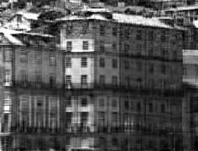
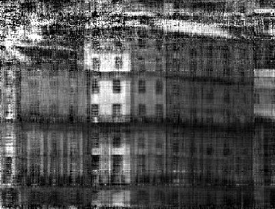
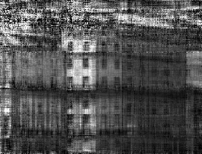
A hyperspectral image is a tensor whose the slices are photographs of the same scene under different wavelets. We adopt the dataset provided in Foster et al. (2006) which contains images about eight different rural scenes taken under 33 various wavelets. To make all methods in our baseline applicable to the completion problem, we resize each hyperspectral images to a small dimension such that $n_{1}=306$, $n_{2}=402$, and $n_{3}=33$. Empirically, we treat these graphs as tensors of rank $r=(30,30,6)$. The observed pixels, or the training set, are sampled from the tensors uniformly at random. And the sample size is set to $|\Omega|=OS\times p$ in which $OS$ is so-called Over-Sampling ratio and $p=\sum_{i=1}^{3}(n_{i}r_{i}-r_{i}^{2})+r_{1}r_{2}r_{3}$ is the number of free parameters in a size $n$ tensor with rank $r$. In addition to the observed entries, the mode-$1$ feature matrix is constructed by extracting the top-$(r_{1}+10)$ singular vectors from a matrix of size $n_{1}\times 10r_{1}$ whose columns are sampled from the mode-1 fibers of the hyperspectral graphs. The recovery accuracy is measured by Normalized Root Mean Square Error (NRMSE)  Kressner et al. (2014). All the compared methods are terminated when the training NRMSE is less than $0.003$ or iterate more than $300$ epochs. We report the NRMSE and CPU time of the compared methods in Tab. 2. From the table, we can see that the proposed method has much higher accuracy than the other solvers in our baseline. The empirical results also indicate that our method has nearly the same running time with FTC, the fastest tensor completion method. The visual results of the 27th slices of recovered hyperspectral images of scene 7 are illustrated in Fig. 2.

Table 2: Performance of the compared methods on hyperspectral images.
AltMin FTC GeomCG gHOI HalRTC RUBIK TFAI CGSI
data OS NRMSE Time(s) NRMSE Time NRMSE Time NRMSE Time NRMSE Time NRMSE Time NRMSE Time NRMSE Time
Scene1 3 0.161 183 0.091 52 0.113 61 0.115 65 0.080 177 0.086 197 0.161 164 0.062 77
5 0.156 307 0.067 76 0.077 93 0.103 109 0.078 177 0.085 194 0.159 273 0.040 100
7 0.156 429 0.060 100 0.056 124 0.092 152 0.077 177 0.085 195 0.159 382 0.039 110
9 0.156 550 0.046 126 0.044 151 0.078 195 0.077 178 0.085 198 0.156 479 0.036 126
Scene2 3 0.173 183 0.093 50 0.114 61 0.125 65 0.066 173 0.061 197 0.173 165 0.048 83
5 0.166 306 0.082 76 0.076 92 0.100 103 0.066 171 0.061 196 0.171 203 0.043 96
7 0.166 428 0.073 101 0.064 123 0.091 152 0.057 172 0.061 197 0.169 386 0.040 110
9 0.166 578 0.062 125 0.056 154 0.073 197 0.057 171 0.060 197 0.169 433 0.038 130
Scene3 3 0.033 226 0.041 68 0.044 181 0.043 187 0.034 174 0.062 189 0.063 131 0.025 83
5 0.033 346 0.030 99 0.029 251 0.037 308 0.033 177 0.061 185 0.062 209 0.021 108
7 0.033 486 0.023 124 0.021 389 0.033 177 0.031 177 0.059 187 0.057 210 0.018 131
9 0.033 587 0.019 156 0.021 386 0.031 491 0.029 172 0.034 189 0.033 229 0.017 143
Scene4 3 0.033 238 0.031 78 0.036 181 0.038 193 0.047 172 0.034 182 0.033 155 0.012 105
5 0.033 359 0.015 108 0.015 254 0.031 293 0.032 171 0.037 183 0.033 247 0.012 118
7 0.033 486 0.012 128 0.012 391 0.021 177 0.029 177 0.027 180 0.033 181 0.011 131
9 0.033 600 0.012 170 0.012 398 0.018 492 0.026 177 0.024 192 0.033 231 0.010 144
Scene5 3 0.059 236 0.051 75 0.077 180 0.169 187 0.086 169 0.126 180 0.062 99 0.024 104
5 0.059 362 0.041 104 0.051 254 0.113 289 0.076 171 0.059 183 0.061 128 0.022 114
7 0.059 483 0.034 137 0.037 325 0.089 398 0.047 173 0.054 190 0.061 181 0.021 128
9 0.059 603 0.028 166 0.029 400 0.065 494 0.042 173 0.058 192 0.061 229 0.021 142
Scene6 3 0.090 237 0.067 76 0.057 181 0.132 189 0.095 177 0.090 180 0.091 170 0.036 107
5 0.090 356 0.039 105 0.040 251 0.095 298 0.083 177 0.081 180 0.091 213 0.034 119
7 0.090 489 0.039 130 0.040 325 0.095 394 0.083 178 0.081 181 0.091 300 0.034 136
9 0.090 600 0.039 165 0.040 396 0.095 501 0.083 178 0.081 183 0.091 383 0.034 143
Scene7 3 0.071 245 0.073 82 0.069 181 0.075 193 0.077 172 0.069 181 0.072 165 0.031 119
5 0.072 377 0.034 102 0.032 225 0.064 293 0.069 172 0.067 180 0.072 203 0.028 158
7 0.072 581 0.028 161 0.028 336 0.052 452 0.062 171 0.064 181 0.072 302 0.026 157
9 0.072 603 0.027 170 0.027 400 0.041 494 0.057 173 0.058 183 0.072 183 0.026 189
Scene8 3 0.039 236 0.030 74 0.042 181 0.050 187 0.071 174 0.034 179 0.040 131 0.013 103
5 0.039 354 0.018 107 0.019 247 0.038 293 0.061 174 0.040 182 0.045 213 0.012 114
7 0.039 701 0.013 102 0.013 381 0.030 234 0.031 181 0.030 182 0.060 363 0.011 169
9 0.039 853 0.012 112 0.012 502 0.026 369 0.027 175 0.031 183 0.039 502 0.011 180
Original Observed CGSI RUBIK FTC
Refer to caption Refer to caption Refer to caption Refer to caption Refer to caption
Figure 2: Visual results of the recovered 27th frame of scene7 when OS is set to 3.

V.2 Recommender System

In recommendation tasks, two datasets are considered: MovieLens 10M (ML10M) and MovieLens 20M (ML20M). Both datasets contain the rating history of users for items at specific moments. For both datasets, we partition the samples into 731 slices in terms of time stamp. Those slices have the identical time intervals. Accordingly, the completion tasks for the two datasets are of sizes $71567\times 10681\times 731$ and $138493\times 26744\times 731$ respectively. In addition to the rating history, both datasets contain two extra files: one describes the genres of each movie, and the other contains tags of each movie. We construct a corpus that contains the text description of all movies from the genres descriptions and all the tags. The feature matrix is extracted from the above corpus by the latent semantic analysis (LSA) method. The processing is efficient since LSA is implemented via randomized SVD.

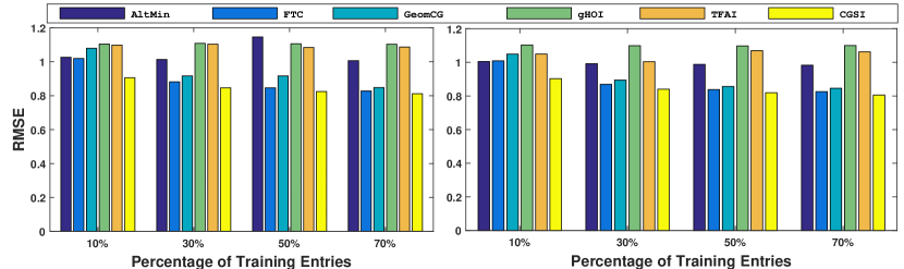
Various empirical studies are conducted to validate the performance of the proposed method. In the first scenario, we record the CPU time and the Root Mean Square Error (RMSE) outputted by the compared algorithms under different choices of multi-linear rank. In this scenario, for both datasets, $80\%$ samples are chosen as training set, and the rest are left for testing. The results are listed in Tab. 3, which suggests that the proposed method outperforms all other solvers in terms of accuracy. For ML10M, our method uses significantly less CPU time than its competitors. In Fig. 4, we report another scenario, in which the percentage of training samples are varied from $10\%$ to $70\%$ and the rank parameter is fixed to $(10,10,10)$. Experimental results in this figure indicate that our method has the lowest RMSE.

To show the impact of parameter $\alpha$ on the performance of our method, we depict the relation between RMSE and $\alpha$ in Fig. 3, where the rank parameter is set to $(10,10,10)$, and the partitioning scheme for training and testing samples is the same as the first scenario. From this Figure we can see that our method has higher accuracy than the vanilla Riemannian model’s solver FTC for a wide range of parameter choices.

Refer to caption
Figure 3: Effect of parameter $\alpha$ on the accuracy of CGSI.
Table 3: Performance of the compared methods on Recommendation Tasks.
AltMin FTC GeomCG gHOI TFAI CGSI
dataset rank RMSE Time(s) RMSE Time RMSE Time RMSE Time RMSE Time RMSE Time
ML10M (4,4,4) 0.982 924 0.824 236 0.835 307 1.076 467 1.011 426 0.823 178
(6,6,6) 0.968 1830 0.814 535 0.826 679 1.262 1035 0.9948 942 0.814 434
(8,8,8) 1.01 3123 0.822 928 0.833 1135 1.062 1734 0.993 1617 0.810 754
(10,10,10) 1.147 4963 0.824 1631 0.843 2220 1.094 2788 0.992 2522 0.807 1067
ML20M (4,4,4) 1.061 690 0.822 466 0.829 601 1.050 918 1.029 797 0.818 363
(6,6,6) 1.089 3451 0.808 982 0.822 1309 1.057 1869 1.008 1644 0.805 1107
(8,8,8) 1.092 5890 0.812 1725 0.828 2271 1.045 3363 1.004 3144 0.804 1739
(10,10,10) 1.092 9418 0.818 3161 0.834 4308 1.054 5795 1.025 5394 0.799 2813
Refer to caption
Figure 4: Accuracy of compared methods under different size of training set

VI.   Conclusion

In this paper, we exploit the side information to improve the accuarcy of Riemannian tensor completion. A novel Riemanian model is proposed. To solve the model efficiently, we design a new Riemannian metric. Such metric will induce an adaptive preconditioner for the solvers of the proposed model. Then, we devise a Riemannian conjugate gradient descent method using the adaptive preconditioner. Empirical results show that our solver outperforms state-of-the-arts.

VII.   appendix

VII.1 Proof of Propositions

Before delve into the proofs of the propositions, we construct the submersion between the total space ${\mathcal{M}_{r}}$ and fix multilinear rank manifold $\mathcal{F}_{r}$ in the following Lemma.

Lemma 5.

Let $\pi:{\mathcal{M}_{r}}\rightarrow\mathcal{F}_{r}$ be a mapping defined by

$$\pi({\mathbfcal{G}},\mathbf{U}_{1},\mathbf{U}_{2},\mathbf{U}_{3})={\mathbfcal{G}}\times_{i=1}^{3}\mathbf{U}_{i}.$$

Then it is a submersion from ${\mathcal{M}_{r}}$ to $\mathcal{F}_{r}$.

Proof.

To begin with, we define a function $\pi:{\mathcal{M}_{r}}\rightarrow\mathcal{F}_{r}$ as follows

$$\pi({\mathbfcal{G}},\mathbf{U}_{1},\mathbf{U}_{2},\mathbf{U}_{3})={\mathbfcal{G}}\times_{i=1}^{3}\mathbf{U}_{i}.$$

Note that $\pi()$ is a smooth function over ${\mathcal{M}_{r}}$, and for all ${\overline{\mathbfcal{X}}}=({\mathbfcal{G}},\mathbf{U}_{1},\mathbf{U}_{2},\mathbf{U}_{3})\in{\mathcal{M}_{r}}$, and for all the tangent vectors $\eta_{\overline{\mathbfcal{X}}}=(\eta_{\mathbfcal{G}},\eta_{1},\eta_{2},\eta_{3})\in T_{\overline{\mathbfcal{X}}}{\mathcal{M}_{r}}$, the first order derivative of $\pi()$ can be computed as follows:

$$D\pi({\overline{\mathbfcal{X}}})[\eta_{\overline{\mathbfcal{X}}}]=\eta_{\mathbfcal{G}}\times_{i=1}^{3}\mathbf{U}_{i}+{\mathbfcal{G}}\times_{1}\eta_{1}\times_{2}\mathbf{U}_{2}\times_{3}\mathbf{U}_{3}+{\mathbfcal{G}}\times_{1}\mathbf{U}_{1}\times_{2}\eta_{2}\times_{3}\mathbf{U}_{3}+{\mathbfcal{G}}\times_{1}\mathbf{U}_{1}\times_{2}\mathbf{U}_{2}\times_{3}\eta_{3}$$ (14)

Note that $\eta_{G}\in\mathbb{R}^{r_{1}\times r_{2}\times r_{3}}$ and $\eta_{i}\in T_{\mathbf{U}_{i}}\mathop{\rm St}(r_{i},n_{i})$ which means they can be expressed as $\eta_{i}=\mathbf{U}_{i}\mathbf{\Omega}_{i}+\mathbf{U}_{i,\perp}\mathbf{K}_{i}$ where $\Omega_{i}\in\mathbb{R}^{r_{i}\times r_{i}}$ is a skew matrix, $\mathbf{K}_{i}\in\mathbb{R}^{(n_{i}-r_{i})\times r_{i}}$ and $\mathbf{U}_{i,\perp}\in\mathbb{R}^{n_{i}\times(n_{i}-r_{i})}$ is the orthogonal basis, the spanned subspace of which is the orthogonal complement of $\mathop{\rm span}(\mathbf{U}_{i})$. Substitute these expressions to equation (14), we have:

$\displaystyle D\pi({\overline{\mathbfcal{X}}})[\eta_{\overline{\mathbfcal{X}}}]=(\eta_{\mathbfcal{G}}+\sum_{i=1}^{3}{\mathbfcal{G}}\times_{i}\mathbf{\Omega}_{i})\times_{i=1}^{3}\mathbf{U}_{i}+\sum_{i=1}^{3}{\mathbfcal{G}}\times_{i}\mathbf{U}_{i,\perp}\mathbf{K}_{i}\times_{j\neq i,1\leq j\leq 3}\mathbf{U}_{j}.$ (15)

Therefore, the range of the map $D\pi({\overline{\mathbfcal{X}}})[\cdot]$ over the tangent space $T_{\overline{\mathbfcal{X}}}{\mathcal{M}_{r}}$

$\displaystyle\mathop{\rm range}(D\pi({\overline{\mathbfcal{X}}}))=\left\{{\mathbfcal{H}}\times_{i=1}^{3}\mathbf{U}_{i}+\sum_{i=1}^{3}{\mathbfcal{G}}\times_{i}\mathbf{U}_{i,\perp}\mathbf{K}_{i}\times_{j\neq i,1\leq j\leq 3}\mathbf{U}_{j}|{\mathbfcal{H}}\in\mathbb{R}^{r_{1}\times r_{2}\times r_{3}},\mathbf{K}_{i}\in\mathbb{R}^{(n_{i}-r_{i})\times r_{i}}\right\}$ (16)

Note that the tangent space of fix multilinear rank manifold $\mathcal{F}_{r}$ at the point 𝒳π𝒢𝒰𝒰𝒰𝒳𝜋𝒢subscript𝒰subscript𝒰subscript𝒰\mathbfcal{X}=\pi({\mathbfcal{G}},\mathbf{U}_{1},\mathbf{U}_{2},\mathbf{U}_{3}) is

$$T_{\mathbfcal{X}}\mathcal{F}_{r}=\left\{{\mathbfcal{H}}\times_{i=1}^{3}\mathbf{U}_{i}+\sum_{i=1}^{3}{\mathbfcal{G}}\times_{i}\mathbf{V}_{i}\times_{j\neq i,1\leq j\leq 3}\mathbf{U}_{j}|{\mathbfcal{H}}\in\mathbb{R}^{r_{1}\times r_{2}\times r_{3}},\mathbf{V}_{i}\in\mathbb{R}^{n_{i}\times r_{i}}\text{ and }\mathbf{V}_{i}\mathbf{U}_{i}=\mathbf{0}\right\}.$$ (17)

Using the fact any matrix $\mathbf{V}_{i}\in\mathbb{R}^{n_{i}\times r_{i}}$ and $\mathbf{V}_{i}^{\top}\times\mathbf{U}_{i}=\mathbf{0}$, there exist $\mathbf{K}_{i}\in\mathbb{R}^{(n_{i}-r_{i})\times r_{i}}$ such that $\mathbf{V}_{i}=\mathbf{U}_{i,\perp}\mathbf{K}_{i}$, we can infer that

$$\mathop{\rm range}(D\pi({\overline{\mathbfcal{X}}}))=T_{\mathbfcal{X}}\mathcal{F}_{r}.$$ (18)

As a result, $\pi(\cdot)$ is a submersion from ${\mathcal{M}_{r}}$ to $\mathcal{F}_{r}$. ∎

VII.1.1 Horizontal Space

Proposition 6.

Let ${\overline{\mathbfcal{X}}}=({\mathbfcal{G}},\mathbf{U}_{1},\mathbf{U}_{2},\mathbf{U}_{3})\in[\mathbfcal{X}]$, the horizontal space of ${\mathcal{M}_{r}}$ at point ${\overline{\mathbfcal{X}}}$ is

$$\big{\{}\eta_{{\overline{\mathbfcal{X}}}}\in T_{{\overline{\mathbfcal{X}}}}{\mathcal{M}_{r}}|\mathbf{V}_{i}^{\top}\eta_{i}\mathbf{G}_{i}+\mathbf{W}_{i}^{\top}\eta_{i}\mathbf{G}_{\alpha_{i}}\text{is symmetric}\forall 1\leq i\leq 3\big{\}}$$

where $\mathbf{V}_{i}=\mathbf{P}_{i}\mathbf{P}_{i}^{\top}\mathbf{U}_{i}$, $\mathbf{W}_{i}=\mathbf{U}_{i}-\mathbf{P}_{i}\mathbf{P}_{i}^{\top}\mathbf{U}_{i}$, $\mathbf{G}_{i}={\mathbfcal{G}}_{(i)}{\mathbfcal{G}}_{(i)}^{\top}$, $\mathbf{G}_{\alpha_{i}}=N\alpha_{i}\mathbf{I}_{i}+{\mathbfcal{G}}_{(i)}{\mathbfcal{G}}_{(i)}^{\top}$.

Proof.

Let $\mathbfcal{X}\in\mathcal{F}_{r}$ be a tensor with tucker factorization ${\overline{\mathbfcal{X}}}=({\mathbfcal{G}},\mathbf{U}_{1},\mathbf{U}_{2},\mathbf{U}_{3})\in[\mathbfcal{X}]$. In quotient manifold framework Absil et al. (2009), the equivalent class $[\mathbfcal{X}]$ is called the fiber of total space. The lifted representation of the tangent space $T_{[\mathbfcal{X}]}{\mathcal{M}_{r}}/\sim$ is identified with a subspace of the tangent space $T_{{\overline{\mathbfcal{X}}}}{\mathcal{M}_{r}}$ that does not produce a displacement along the fiber $[\mathbfcal{X}]$. This is realized by decomposing $T_{{\overline{\mathbfcal{X}}}}{\mathcal{M}_{r}}$ into two complementary subspace, the vertical and horizontal spaces, such that $T_{{\overline{\mathbfcal{X}}}}{\mathcal{M}_{r}}={\mathcal{H}_{{\overline{\mathbfcal{X}}}}}\oplus{\mathcal{V}_{{\overline{\mathbfcal{X}}}}}$, where ${\mathcal{H}_{{\overline{\mathbfcal{X}}}}}$ is the horizontal space and ${\mathcal{V}_{{\overline{\mathbfcal{X}}}}}$ is the vertical space. It should be emphasized that the decomposition is respect to the metric (11). The vertical space ${\mathcal{V}_{{\overline{\mathbfcal{X}}}}}$ is the tangent space of the fiber $[\mathbfcal{X}]$. According to Kasai and Mishra (2016), the vertical space can be expressed as follows.

$${\mathcal{V}_{{\overline{\mathbfcal{X}}}}}=\{(-\sum_{i=1}^{3}{\mathbfcal{G}}\times_{i}\mathbf{\Omega}_{i},\mathbf{U}_{1}\mathbf{\Omega}_{1},\mathbf{U}_{2}\mathbf{\Omega}_{2},\mathbf{U}_{3}\mathbf{\Omega}_{3})|\mathbf{\Omega}_{i}^{\top}=-\mathbf{\Omega}_{i}\}.$$ (19)

Since horizontal space ${\mathcal{H}_{{\overline{\mathbfcal{X}}}}}$ is an orthogonal complement of ${\mathcal{V}_{{\overline{\mathbfcal{X}}}}}$ with respect to the Riemannian metric (11), for all horizontal vectors $\eta_{{\overline{\mathbfcal{X}}}}=(\eta_{\mathbfcal{G}},\eta_{1},\eta_{2},\eta_{3})\in{\mathcal{H}_{{\overline{\mathbfcal{X}}}}}$ we have

$$\langle\eta_{{\overline{\mathbfcal{X}}}},\zeta\rangle_{{\overline{\mathbfcal{X}}}}=0,\forall\zeta\in{\mathcal{V}_{{\overline{\mathbfcal{X}}}}}.$$ (20)

Using the expression for the horizontal space, the above equation is equivalent to the following one:

$\displaystyle\sum_{i=1}^{3}\langle{\eta_{i}},\mathbf{U}_{i}\mathbf{\Omega}_{i}{\mathbfcal{G}}_{(i)}{\mathbfcal{G}}_{(i)}^{\top}\rangle+\langle{\eta_{\mathbfcal{G}}},-\sum_{i=1}^{3}{\mathbfcal{G}}\times_{i}\mathbf{\Omega}_{i}\rangle$ (21)
$\displaystyle\quad+\sum_{i=1}^{3}N\alpha_{i}\langle{\eta_{i}},(\mathbf{I}_{i}-\mathbf{P}_{i}\mathbf{P}_{i}^{\top})\mathbf{U}_{i}\Omega_{i}\rangle=0.$

Using the property for the Euclidean inner product that for matrix $\mathbf{A},\mathbf{B},\mathbf{C},\mathbf{D}$ we have $\langle\mathbf{A},\mathbf{B}\mathbf{C}\mathbf{D}\rangle=\langle\mathbf{B}^{\top}\mathbf{A}\mathbf{D}^{\top},\mathbf{C}\rangle$. And for tensor ${\mathbfcal{A}},{\mathbfcal{B}}$ and matrix $\mathbf{C}$ we have $\langle{\mathbfcal{A}},{\mathbfcal{B}}\times_{i}\mathbf{C}\rangle=\langle{\mathbfcal{A}}_{(i)}{\mathbfcal{B}}_{(i)}^{\top},\mathbf{C}\rangle$. The above equation (22) is equivalent to the following one

$\displaystyle\sum_{i=1}^{3}\big{\langle}\mathbf{U}_{i}^{\top}\eta_{i}{\mathbfcal{G}}_{(i)}{\mathbfcal{G}}_{(i)}^{\top}+\eta_{{\mathbfcal{G}}}{\mathbfcal{G}}_{(i)}^{\top}+N\alpha_{i}(\mathbf{U}_{i}-\mathbf{P}_{i}\mathbf{P}_{i}^{\top}\mathbf{U}_{i})^{\top}\eta_{i},\mathbf{\Omega}_{i}\big{\rangle}=0,\forall\text{skew matrix }\mathbf{\Omega}_{i}$ (22)

Thus we have $\eta_{{\overline{\mathbfcal{X}}}}$ satisfy the following conditions

$\displaystyle(\mathbf{P}_{i}\mathbf{P}_{i}^{\top}\mathbf{U}_{i})^{\top}\eta_{i}{\mathbfcal{G}}_{(i)}{\mathbfcal{G}}_{(i)}^{\top}+(\mathbf{U}_{i}-\mathbf{P}_{i}\mathbf{P}_{i}^{\top}\mathbf{U}_{i})^{\top}\eta_{i}(N\alpha_{i}\mathbf{I}_{i}+{\mathbfcal{G}}_{(i)}{\mathbfcal{G}}_{(i)}^{\top})\text{ is a symmetric matrix}\forall i\in\{1,2,3\}.$ (23)

Defining $\mathbf{V}_{i}:=\mathbf{P}_{i}\mathbf{P}_{i}^{\top}\mathbf{U}_{i}$, $\mathbf{W}_{i}:=\mathbf{U}_{i}-\mathbf{P}_{i}\mathbf{P}_{i}^{\top}\mathbf{U}_{i}$, $\mathbf{G}_{i}:={\mathbfcal{G}}_{(i)}{\mathbfcal{G}}_{(i)}^{\top}$, $\mathbf{G}_{\alpha_{i}}:=N\alpha_{i}\mathbf{I}_{i}+{\mathbfcal{G}}_{(i)}{\mathbfcal{G}}_{(i)}^{\top}$, we obtain the formula for the horizontal space:

$\displaystyle{\mathcal{H}_{{\overline{\mathbfcal{X}}}}}=\big{\{}\eta_{{\overline{\mathbfcal{X}}}}\in T_{{\overline{\mathbfcal{X}}}}{\mathcal{M}_{r}}|\mathbf{V}_{i}^{\top}\eta_{i}\mathbf{G}_{i}+\mathbf{W}_{i}^{\top}\eta_{i}\mathbf{G}_{\alpha_{i}}\text{is symmetric}\big{\}}$ (24)

VII.1.2 Proof of Prop. (1)

Suppose $\mathbfcal{X}$ has tucker factors $({\mathbfcal{G}},\mathbf{U}_{1},\mathbf{U}_{2},\mathbf{U}_{3})$, then one can certify that:

$$\pi^{-1}({\overline{\mathbfcal{X}}})=[{\mathbfcal{G}},\mathbf{U}_{1},\mathbf{U}_{2},\mathbf{U}_{3}].$$

And hence the equivalent relationship $\sim$ defined by the equivalent classes $[{\mathbfcal{G}},\mathbf{U}_{1},\mathbf{U}_{2},\mathbf{U}_{3}]$ can also be expressed in terms of the map $\pi(\cdot)$:

$$({\mathbfcal{G}},\mathbf{U}_{1},\mathbf{U}_{2},\mathbf{U}_{3})\sim({\mathbfcal{H}},\mathbf{V}_{1},\mathbf{V}_{2},\mathbf{V}_{3})\text{ if and only if }\pi({\mathbfcal{G}},\mathbf{U}_{1},\mathbf{U}_{2},\mathbf{U}_{3})=\pi({\mathbfcal{H}},\mathbf{V}_{1},\mathbf{V}_{2},\mathbf{V}_{3}).$$

Since $\pi(\cdot)$ is a submersion (see Lemma 5), by the submersion theorem (Prop. 3.5.23 of Abraham et al. (2012)), the equivalent relation $\sim$ defined by the equivalent classes is regular and the quotient manifold ${\mathcal{M}_{r}}/\sim$ is diffeomorphic to $\mathcal{F}_{r}$. And according to the proof of Prop. 3.5.23 of  Abraham et al. (2012), the mapping $\varrho([{\mathbfcal{G}},\mathbf{U}_{1},\mathbf{U}_{2},\mathbf{U}_{3}])={\mathbfcal{G}}\times_{i=1}^{3}\mathbf{U}_{i}$ defines the diffeomorphism from ${\mathcal{M}_{r}}/\sim$ to $\mathcal{F}_{r}$. Therefore, ρ(𝒳ϱ𝒳𝒢𝒰𝒰𝒰\rho(\mathbfcal{X})=\varrho^{-1}(\mathbfcal{X})=[{\mathbfcal{G}},\mathbf{U}_{1},\mathbf{U}_{2},\mathbf{U}_{3}], where $[{\mathbfcal{G}},\mathbf{U}_{1},\mathbf{U}_{2},\mathbf{U}_{3}]$ is the tucker representation of $\mathbfcal{X}$.

VII.1.3 Proof of Proposition 2

Let ${\overline{\mathbfcal{X}}}=({\mathbfcal{G}},\mathbf{U}_{1},\mathbf{U}_{2},\mathbf{U}_{3})$ be any tucker factors of tensor ${\overline{\mathbfcal{X}}}\in\mathcal{F}_{r}$. According to the definition of Chordal distance of subspaces of different dimension Ye and Lim (2014), we have

$\displaystyle{\mathop{\rm dist}}^{2}(\mathop{\rm span}(\mathbfcal{X}_{(i)}),\mathop{\rm span}(\mathbf{P}_{i}))$ $\displaystyle=$ $\displaystyle{\mathop{\rm dist}}^{2}(\mathop{\rm span}(\mathbf{U}_{i}),\mathop{\rm span}(\mathbf{P}_{i}))$ (25)
$\displaystyle=$ $\displaystyle\sum_{i=1}^{r_{i}}\sin^{2}(\theta_{i})+k_{i}-r_{i}$ (26)
$\displaystyle=$ $\displaystyle\sum_{i=1}^{r_{i}}(1-\cos^{2}(\theta_{i}))+k_{i}-r_{i}$ (27)
$\displaystyle=$ $\displaystyle\mathop{\rm trace}(\mathbf{I})-\|\mathbf{P}_{i}^{\top}\mathbf{U}_{i}\|_{F}^{2}+k_{i}-r_{i}$ (28)
$\displaystyle=$ $\displaystyle\mathop{\rm trace}(\mathbf{U}_{i}^{\top}(\mathbf{I}-\mathbf{P}_{i}^{\top}\mathbf{P}_{i})\mathbf{U}_{i})+k_{i}-r_{i}$ (29)

where in the second equation $\theta_{i}$ is the $i$-th principal angle between $\mathop{\rm span}{\mathbf{U}_{i}}$ and $\mathop{\rm span}{\mathbf{P}_{i}}$, the second equation is derived from the definition of Chordal distance, the fourth equation is derived from the fact that $\cos(\theta_{i})$ is the $i$-th singular value of $\mathbf{P}_{i}^{\top}\mathbf{Q}_{i}$ due to $\mathbf{P}_{i}$ and $\mathbf{Q}_{i}$ are orthogonal bases (see Alg 12.4.3 of Golub and Van Loan (2012)). Therefore for all $({\mathbfcal{G}},\mathbf{U}_{1},\mathbf{U}_{2},\mathbf{U}_{3})\in{\mathcal{M}_{r}}$, we have

$$l(\pi({\mathbfcal{G}},\mathbf{U}_{1},\mathbf{U}_{2},\mathbf{U}_{3}))=\frac{1}{2}\|{\mathbf{\mathcal{P}}_{\Omega}}({\mathbfcal{G}}\times_{i=1}^{3}\mathbf{U}_{i}-{\mathbfcal{R}})\|_{F}^{2}+\sum_{i=1}^{3}(\mathop{\rm trace}(\mathbf{U}_{i}^{\top}(\mathbf{I}-\mathbf{P}_{i}^{\top}\mathbf{P}_{i})\mathbf{U}_{i})+k_{i}-r_{i}).$$ (30)

Which is equivalent to:

$$l(\pi({\mathbfcal{G}},\mathbf{U}_{1},\mathbf{U}_{2},\mathbf{U}_{3}))=f({\mathbfcal{G}},\mathbf{U}_{1},\mathbf{U}_{2},\mathbf{U}_{3})+C$$ (31)

where $C=\sum_{i=1}^{3}(k_{i}-r_{i})$ is a constant.

Note that the critical points of a function $h(x)$ over a smooth manifold $\mathcal{M}$ are those whose Riemannian gradient vanishing, that is $\mathop{\rm grad}h(x)=0$. And one can show that:

$$\mathop{\rm grad}h(x)=0\text{ if and only if }Dh(x)[\eta_{x}]=0\forall\eta_{x}\in T_{x}\mathcal{M}.$$ (32)

To prove that $\mathbfcal{X}$ is a critical point of $l(\cdot)$ over $\mathcal{F}_{r}$ if and only if $[\mathbfcal{X}]$ is a critical point of $\tilde{f}(\cdot)$ over ${\mathcal{M}_{r}}/\sim$, we need to prove that

gradl(𝒳 if and only if }{~𝒳\mathop{\rm grad}l(\mathbfcal{X})=\mathbf{0}\text{ if and only if }\mathop{\rm grad}\tilde{f}([\mathbfcal{X}])=\mathbf{0}. (33)

Note that since $\mathop{\rm grad}f({\mathbfcal{G}},\mathbf{U}_{1},\mathbf{U}_{2},\mathbf{U}_{3})$ is the horizontal lift of $\mathop{\rm grad}\tilde{f}([\mathbfcal{X}])$ for all $({\mathbfcal{G}},\mathbf{U}_{1},\mathbf{U}_{2},\mathbf{U}_{3})\in[\mathbfcal{X}]$. We have gradf~([𝒳\mathop{\rm grad}\tilde{f}([\mathbfcal{X}])=\mathbf{0} if and only if $\mathop{\rm grad}f({\mathbfcal{G}},\mathbf{U}_{1},\mathbf{U}_{2},\mathbf{U}_{3})=0$ for at least one $({\mathbfcal{G}},\mathbf{U}_{1},\mathbf{U}_{2},\mathbf{U}_{3})\in[\mathbfcal{X}]$. Thus to prove (33), one only need to certify

gradl(𝒳 if and only if 𝒢𝒰𝒰𝒰𝒳 such that }{𝒢𝒰𝒰𝒰\mathop{\rm grad}l(\mathbfcal{X})=\mathbf{0}\text{ if and only if }\exists({\mathbfcal{G}},\mathbf{U}_{1},\mathbf{U}_{2},\mathbf{U}_{3})\in[\mathbfcal{X}]\text{ such that }\mathop{\rm grad}f({\mathbfcal{G}},\mathbf{U}_{1},\mathbf{U}_{2},\mathbf{U}_{3})=\mathbf{0}. (34)

On one side, suppose gradl(𝒳\mathop{\rm grad}l(\mathbfcal{X})=\mathbf{0}, and ${\overline{\mathbfcal{X}}}=({\mathbfcal{G}},\mathbf{U}_{1},\mathbf{U}_{2},\mathbf{U}_{3})\in[\mathbfcal{X}]$. Let $\eta_{\overline{\mathbfcal{X}}}$ be any tangent vector belonging to $T_{{\overline{\mathbfcal{X}}}}{\mathcal{M}_{r}}$. We have:

$\displaystyle Df({\overline{\mathbfcal{X}}})[\eta_{\overline{\mathbfcal{X}}}]$ $\displaystyle=$ $\displaystyle Dl(\pi({\overline{\mathbfcal{X}}}))[D\pi({\overline{\mathbfcal{X}}})[\eta_{\overline{\mathbfcal{X}}}]]$ (35)
$\displaystyle=$ $\displaystyle Dl(\mathbfcal{X})[D\pi({\overline{\mathbfcal{X}}})[\eta_{\overline{\mathbfcal{X}}}]]$ (36)
$\displaystyle=$ $\displaystyle 0$ (37)

where the first equation is derived from equation (31) and chain rule of first order derivative; the third equation is due to gradl(𝒳\mathop{\rm grad}l(\mathbfcal{X})=\mathbf{0} and $D\pi({\overline{\mathbfcal{X}}})[\eta_{\overline{\mathbfcal{X}}}]\in T_{\mathbfcal{X}}\mathcal{F}_{r}$ since $\pi(\cdot)$ is a submersion (See Lemma 5). Because $\eta_{\overline{\mathbfcal{X}}}$ is an arbitrary tangent vector, we have

$$Df({\overline{\mathbfcal{X}}})[\eta_{\overline{\mathbfcal{X}}}]=0\forall\eta_{\overline{\mathbfcal{X}}}\in T_{{\overline{\mathbfcal{X}}}}{\mathcal{M}_{r}}.$$ (38)

And according to (32) we have $\mathop{\rm grad}f({\overline{\mathbfcal{X}}})=\mathbf{0}$. Thus, we prove that

gradl(𝒳}{𝒳¯\mathop{\rm grad}l(\mathbfcal{X})=\mathbf{0}\Rightarrow\mathop{\rm grad}f({\overline{\mathbfcal{X}}})=0. (39)

On the other side, suppose ${\overline{\mathbfcal{X}}}=({\mathbfcal{G}},\mathbf{U}_{1},\mathbf{U}_{2},\mathbf{U}_{3})\in[\mathbfcal{X}]$ and $\mathop{\rm grad}f({\overline{\mathbfcal{X}}})=\mathbf{0}$. Then for all $\eta{X}\in T{X}\mathcal{F}_{r}$ we have:

$\displaystyle Dl(\mathbfcal{X})[\eta{X}]$ $\displaystyle=$ $\displaystyle Dl(\pi({\overline{\mathbfcal{X}}}))[\eta{X}]$ (40)
$\displaystyle=$ $\displaystyle Dl(\pi({\overline{\mathbfcal{X}}}))[D\pi({\overline{\mathbfcal{X}}})[\eta_{\overline{\mathbfcal{X}}}]]$ (41)
$\displaystyle=$ $\displaystyle Df({\overline{\mathbfcal{X}}})(\eta_{\overline{\mathbfcal{X}}})$ (42)
$\displaystyle=$ $\displaystyle 0$ (43)

where the second equation is because there exist $\eta_{\overline{\mathbfcal{X}}}\in T_{{\overline{\mathbfcal{X}}}}{\mathcal{M}_{r}}$ such that $D\pi({\overline{\mathbfcal{X}}})[\eta_{\overline{\mathbfcal{X}}}]=\eta{X}$ due to $\pi()$ being a submersion (See Lemma 5); the third equation is derived by the equation (31) and chain rule of first order derivative; the fourth equation is due to $\mathop{\rm grad}f({\overline{\mathbfcal{X}}})=\mathbf{0}$. Thus we have proved that

gradf(𝒳¯)=0gradl(𝒳\mathop{\rm grad}f({\overline{\mathbfcal{X}}})=0\Rightarrow\mathop{\rm grad}l(\mathbfcal{X})=0 (44)

Since we have proved both (39) and (44), we have (34) holds.

VII.1.4 Proof of Proposition 3

Since the Euclidean ambient space (71) $\mathbb{R}^{r_{1}\times r_{2}\times r_{3}}\times\mathbb{R}^{n_{1}\times r_{1}}\times\mathbb{R}^{n_{2}\times r_{2}}\times\mathbb{R}^{n_{3}\times r_{3}}$ is an special smooth manifold, with tangent space at each its point being the ambient space itself Absil et al. (2009). Therefore, one can endow the ambient space with a metric, and treats it as a Riemannian manifold. By endowing the ambient space with the same metric with total space, namely:

$\displaystyle\langle{\overline{\mathbfcal{X}}},{\overline{\mathbfcal{Y}}}\rangle_{{\overline{\mathbfcal{Z}}}}=\sum_{i=1}^{3}\langle{\overline{\mathbfcal{X}}}_{\mathbf{U}_{i}},{\overline{\mathbfcal{Y}}}_{\mathbf{U}_{i}}({\overline{\mathbfcal{Z}}}_{{\mathbfcal{G}}})_{(i)}({\overline{\mathbfcal{Z}}}_{{\mathbfcal{G}}})_{(i)}^{\top}\rangle+\langle{\overline{\mathbfcal{X}}}_{{\mathbfcal{G}}},{\overline{\mathbfcal{Y}}}_{{\mathbfcal{G}}}\rangle+\sum_{i=1}^{3}N\alpha_{i}\langle{\overline{\mathbfcal{X}}}_{\mathbf{U}_{i}},(\mathbf{I}_{i}-\mathbf{P}_{i}\mathbf{P}_{i}^{\top}){\overline{\mathbfcal{Y}}}_{\mathbf{U}_{i}}\rangle$ (45)

where ${\overline{\mathbfcal{X}}},{\overline{\mathbfcal{Y}}},{\overline{\mathbfcal{Z}}}$ are any ambient vectors, and all of them are tuples like $({\overline{\mathbfcal{X}}}_{{\mathbfcal{G}}},{\overline{\mathbfcal{X}}}_{\mathbf{U}_{1}},{\overline{\mathbfcal{X}}}_{\mathbf{U}_{2}},{\overline{\mathbfcal{X}}}_{\mathbf{U}_{3}})$. The scaled Euclidean of the cost $\tilde{\nabla}f({\overline{\mathbfcal{X}}})$ means the ambient vector which satisfies the following condition

$$\langle\tilde{\nabla}f({\overline{\mathbfcal{X}}}),{\overline{\mathbfcal{Y}}}\rangle_{\overline{\mathbfcal{X}}}=Df({\overline{\mathbfcal{X}}})[{\overline{\mathbfcal{Y}}}],\forall{\overline{\mathbfcal{Y}}}\in\text{ambient space}$$ (46)

This equation is equivalent to the following:

$$\begin{aligned} &\sum_{i=1}^{3}\langle{\overline{\mathbfcal{Y}}}_{i},\tilde{\nabla}_{\mathbf{U}_{i}}f({\overline{\mathbfcal{X}}})({\overline{\mathbfcal{X}}}_{{\mathbfcal{G}}})_{(i)}({\overline{\mathbfcal{X}}}_{{\mathbfcal{G}}})_{(i)}^{\top}\rangle+\langle{\overline{\mathbfcal{Y}}}_{\mathbfcal{G}},\tilde{\nabla}_{{\mathbfcal{G}}}f({\overline{\mathbfcal{X}}})\rangle+\sum_{i=1}^{3}N\alpha_{i}\langle{\overline{\mathbfcal{Y}}}_{i},(\mathbf{I}_{i}-\mathbf{P}_{i}\mathbf{P}_{i}^{\top})\tilde{\nabla}_{\mathbf{U}_{i}}f({\overline{\mathbfcal{X}}})\rangle\\ &=\sum_{i=1}^{3}\langle{\overline{\mathbfcal{Y}}}_{i},\nabla_{\mathbf{U}_{i}}\bar{f}({\overline{\mathbfcal{X}}})\rangle+\langle{\overline{\mathbfcal{Y}}}_{{\mathbfcal{G}}},\nabla_{{\mathbfcal{G}}}\bar{f}({\overline{\mathbfcal{X}}})\rangle,\forall{\overline{\mathbfcal{Y}}}\in\text{ ambient space}\end{aligned}.$$ (47)

By taking the partial Euclidean gradient both side of above equation with respect to ${\overline{\mathbfcal{Y}}}_{{\mathbfcal{G}}}$ and ${\overline{\mathbfcal{Y}}}_{\mathbf{U}_{i}}$, one has

$\displaystyle\tilde{\nabla}_{{\mathbfcal{G}}}\bar{f}({\overline{\mathbfcal{X}}})=\nabla_{{\mathbfcal{G}}}\bar{f}({\overline{\mathbfcal{X}}})$ (48)
$\displaystyle\tilde{\nabla}_{\mathbf{U}_{i}}\bar{f}({\overline{\mathbfcal{X}}})=\mathbf{E}_{i}(({\overline{\mathbfcal{X}}}_{{\mathbfcal{G}}})_{(i)}({\overline{\mathbfcal{X}}}_{{\mathbfcal{G}}})_{(i)}^{\top})^{-1}+\mathbf{F}_{i}(N\alpha_{i}\mathbf{I}_{i}+({\overline{\mathbfcal{X}}}_{{\mathbfcal{G}}})_{(i)}({\overline{\mathbfcal{X}}}_{{\mathbfcal{G}}})_{(i)}^{\top})^{-1}$

where $\mathbf{E}_{i}=\mathbf{P}_{i}\mathbf{P}_{i}^{\top}\nabla_{\mathbf{U}_{i}}f({\overline{\mathbfcal{X}}})$ and $\mathbf{F}_{i}=\nabla_{\mathbf{U}_{i}}f({\overline{\mathbfcal{X}}})-\mathbf{E}_{i}$.

VII.1.5 Proof of Proposition 4

According to  Absil et al. (2009), to prove ${\mathcal{M}_{r}}/\sim$ has the structure of Riemannian manifolds, one need to show that for all $[\mathbfcal{X}]\in{\mathcal{M}_{r}}/\sim$ and for all tangent vectors $\eta_{[\mathbfcal{X}]},\xi_{[\mathbfcal{X}]}\in T_{[\mathbfcal{X}]}{\mathcal{M}_{r}}/\sim$ we have

$$\langle\eta_{{\overline{\mathbfcal{X}}}_{1}},\xi_{{\overline{\mathbfcal{X}}}_{1}}\rangle_{{\overline{\mathbfcal{X}}}_{1}}=\langle\eta_{{\overline{\mathbfcal{X}}}_{2}},\xi_{{\overline{\mathbfcal{X}}}_{2}}\rangle_{{\overline{\mathbfcal{X}}}_{2}},\forall{\overline{\mathbfcal{X}}}_{1},{\overline{\mathbfcal{X}}}_{2}\in[\mathbfcal{X}]$$ (49)

where $\eta_{{\overline{\mathbfcal{X}}}_{1}},\eta_{{\overline{\mathbfcal{X}}}_{2}}$ are horizontal lift of $\eta_{[\mathbfcal{X}]}$ and $\xi_{{\overline{\mathbfcal{X}}}_{1}},\xi_{{\overline{\mathbfcal{X}}}_{2}}$ are horizontal lift of $\xi_{[\mathbfcal{X}]}$. To prove that, we firstly express ${\overline{\mathbfcal{X}}}_{2},\eta_{{\overline{\mathbfcal{X}}}_{2}},\xi_{{\overline{\mathbfcal{X}}}_{2}}$ in terms of ${\overline{\mathbfcal{X}}}_{1},\eta_{{\overline{\mathbfcal{X}}}_{1}},\xi_{{\overline{\mathbfcal{X}}}_{1}}$, then verify the invariant property (49).

Let ${\overline{\mathbfcal{X}}}_{1}=({\mathbfcal{G}},\mathbf{U}_{1},\mathbf{U}_{2},\mathbf{U}_{3})$. since ${\overline{\mathbfcal{X}}}_{1},{\overline{\mathbfcal{X}}}_{2}\in[\mathbfcal{X}]$, there exist orthogonal matrices $\mathbf{O}_{i}\in\mathcal{O}(r_{i})$ such that

$${\overline{\mathbfcal{X}}}_{2}=({\mathbfcal{G}}\times_{i=1}^{3}\mathbf{O}_{i}^{\top},\mathbf{U}_{1}\mathbf{O}_{1},\mathbf{U}_{2}\mathbf{O}_{2},\mathbf{U}_{3}\mathbf{O}_{3}).$$ (50)

Let $\eta_{{\overline{\mathbfcal{X}}}_{1}}=(\eta_{{\mathbfcal{G}}},\eta_{1},\eta_{2},\eta_{3})$, in this paragraph, we will prove that $\eta_{{\overline{\mathbfcal{X}}}_{2}}$ can be expressed by the following formula

$$\eta_{{\overline{\mathbfcal{X}}}_{2}}=(\eta_{{\mathbfcal{G}}}\times_{i=1}^{3}\mathbf{O}_{i}^{\top},\eta_{1}\mathbf{O}_{1},\eta_{2}\mathbf{O}_{2},\eta_{3}\mathbf{O}_{3}).$$ (51)

Note that $\eta_{{\overline{\mathbfcal{X}}}_{2}}$ is the horizontal lift of $\eta_{[{\overline{\mathbfcal{X}}}]}$, to prove (51), one only need to show that $(\eta_{{\mathbfcal{G}}}\times_{i=1}^{3}\mathbf{O}_{i}^{\top},\eta_{1}\mathbf{O}_{1},\eta_{2}\mathbf{O}_{2},\eta_{3}\mathbf{O}_{3})$ satisfy the following two conditions (See Sec. 3.6.2 of Absil et al. (2009))

$\displaystyle\zeta$ $\displaystyle\in$ $\displaystyle{\mathbfcal{H}}_{{\overline{\mathbfcal{X}}}_{2}}$ (52)
$\displaystyle D\tau({\overline{\mathbfcal{X}}}_{2})[\zeta]$ $\displaystyle=$ $\displaystyle\eta_{[\mathbfcal{X}]}$ (53)

where for brevity we denote $(\eta_{{\mathbfcal{G}}}\times_{i=1}^{3}\mathbf{O}_{i}^{\top},\eta_{1}\mathbf{O}_{1},\eta_{2}\mathbf{O}_{2},\eta_{3}\mathbf{O}_{3})$ by $\zeta$; the ${\mathbfcal{H}}_{{\overline{\mathbfcal{X}}}}$ is the horizontal space at ${\overline{\mathbfcal{X}}}$ (See Lemma 6 for its expression); $\tau(\cdot)$ is the nature mapping from ${\mathcal{M}_{r}}$ to ${\mathcal{M}_{r}}/\sim$ which is defined by

$$\tau({\overline{\mathbfcal{X}}})=[\mathbfcal{X}]$$

Note that $\tau()$ is a composition of map $\rho(\cdot)$ and map $\pi(\cdot)$ defined in Prop. 1 and Lemma 5, namely

$$\tau({\overline{\mathbfcal{X}}})=\rho(\pi({\overline{\mathbfcal{X}}})).$$ (54)

According to Lemma. 6, ${\mathbfcal{H}}_{{\overline{\mathbfcal{X}}}_{1}}=\{\eta_{{\overline{\mathbfcal{X}}}_{1}}\in T_{{\overline{\mathbfcal{X}}}_{1}}{\mathcal{M}_{r}}|\mathbf{V}_{i}^{\top}\eta_{i}\mathbf{G}_{i}+\mathbf{W}_{i}^{\top}\eta_{i}\mathbf{G}_{\alpha_{i}}\text{ is symmetric}\}$ where $\mathbf{V}_{i}=\mathbf{P}_{i}\mathbf{P}_{i}^{\top}\mathbf{U}_{i},\mathbf{W}_{i}=\mathbf{U}_{i}-\mathbf{V}_{i},\mathbf{G}_{i}={\mathbfcal{G}}_{(i)}{\mathbfcal{G}}_{(i)}^{\top}$ and ${\mathbfcal{G}}_{\alpha_{i}}=N\alpha_{i}\mathbf{I}_{i}+{\mathbfcal{G}}_{(i)}{\mathbfcal{G}}_{(i)}^{\top}$. Using the equation (50), we have:

$${\mathbfcal{H}}_{{\overline{\mathbfcal{X}}}_{2}}=\{\eta_{{\overline{\mathbfcal{X}}}_{2}}\in T_{{\overline{\mathbfcal{X}}}_{2}}{\mathcal{M}_{r}}|\mathbf{O}_{i}^{\top}\mathbf{V}_{i}^{\top}\eta_{i}\mathbf{O}_{i}^{\top}\mathbf{G}_{i}\mathbf{O}_{i}+\mathbf{O}_{i}^{\top}\mathbf{W}_{i}^{\top}\eta_{i}\mathbf{O}_{i}^{\top}\mathbf{G}_{\alpha_{i}}\mathbf{O}_{i}\text{ is symmetric}\}$$ (55)

(Note that when proving the above equation, we use the equations like: $({\mathbfcal{G}}\times_{i=1}^{3}\mathbf{O}_{i}^{\top})_{(1)}=\mathbf{O}_{1}^{\top}{\mathbfcal{G}}_{(1)}(\mathbf{O}_{2}^{\top}\otimes\mathbf{O}_{3}^{\top})^{\top}$ Kolda and Bader (2009) and the properties like $\mathbf{O}_{2}^{\top}\otimes\mathbf{O}_{3}^{\top}$ is orthogonal matrix ). To prove $\zeta\in{\mathbfcal{H}}_{{\overline{\mathbfcal{X}}}_{2}}$, on one hand we noticed that:

$\displaystyle\zeta_{i}^{\top}\mathbf{U}_{i}\mathbf{O}_{i}+\mathbf{O}_{i}^{\top}\mathbf{U}_{i}^{\top}\zeta_{i}$ $\displaystyle=$ $\displaystyle\mathbf{O}_{i}^{\top}\eta_{i}^{\top}\mathbf{U}_{i}\mathbf{O}_{i}+\mathbf{O}_{i}^{\top}\mathbf{U}_{i}^{\top}\eta_{i}\mathbf{O}_{i}$ (56)
$\displaystyle=$ $\displaystyle\mathbf{O}_{i}^{\top}(\eta_{i}^{\top}\mathbf{U}_{i}+\mathbf{U}_{i}^{\top}\eta_{i})\mathbf{O}_{i}$ (57)
$\displaystyle=$ $\displaystyle\mathbf{0}$ (58)

where the first equation use the fact $\zeta_{i}=\eta_{i}\mathbf{O}_{i}$, the third equation use the fact $\eta_{i}\in T_{\mathbf{U}_{i}}\mathop{\rm St}(r_{i},n_{i})$ is equivalent to $\eta_{i}^{\top}\mathbf{U}_{i}+\mathbf{U}_{i}^{\top}\eta_{i}=\mathbf{0}$ (See Sec 3.5.7 of  Absil et al. (2009)). The above equation implies that $\zeta_{i}\in T_{\mathbf{U}_{i}\mathbf{O}_{i}}\mathop{\rm St}(r_{i},n_{i})$. And hence we have

$$\zeta\in\big{(}\mathbb{R}^{r_{1}\times r_{2}\times r_{3}}\times T_{\mathbf{U}_{1}\mathbf{O}_{1}}\mathop{\rm St}(r_{1},n_{1})\times T_{\mathbf{U}_{2}\mathbf{O}_{2}}\mathop{\rm St}(r_{2},n_{2})\times T_{\mathbf{U}_{3}\mathbf{O}_{3}}\mathop{\rm St}(r_{3},n_{3})\big{)}=T_{{\overline{\mathbfcal{X}}}_{2}}{\mathcal{M}_{r}}.$$ (59)

One the other hand, we have $\mathbf{O}_{i}^{\top}\mathbf{V}_{i}^{\top}\zeta_{i}\mathbf{O}_{i}^{\top}\mathbf{G}_{i}\mathbf{O}_{i}+\mathbf{O}_{i}^{\top}\mathbf{W}_{i}^{\top}\zeta_{i}\mathbf{O}_{i}^{\top}\mathbf{G}_{\alpha_{i}}\mathbf{O}_{i}$ is symmetric since:

$\displaystyle(\mathbf{O}_{i}^{\top}\mathbf{V}_{i}^{\top}\zeta_{i}\mathbf{O}_{i}^{\top}\mathbf{G}_{i}\mathbf{O}_{i}+\mathbf{O}_{i}^{\top}\mathbf{W}_{i}^{\top}\zeta_{i}\mathbf{O}_{i}^{\top}\mathbf{G}_{\alpha_{i}}\mathbf{O}_{i})^{\top}$ $\displaystyle=$ $\displaystyle(\mathbf{O}_{i}^{\top}\mathbf{V}_{i}^{\top}\eta_{i}\mathbf{O}_{i}\mathbf{O}_{i}^{\top}\mathbf{G}_{i}\mathbf{O}_{i}+\mathbf{O}_{i}^{\top}\mathbf{W}_{i}^{\top}\eta_{i}\mathbf{O}_{i}\mathbf{O}_{i}^{\top}\mathbf{G}_{\alpha_{i}}\mathbf{O}_{i})^{\top}$
$\displaystyle=$ $\displaystyle\mathbf{O}_{i}^{\top}(\mathbf{V}_{i}^{\top}\eta_{i}\mathbf{G}_{i}+\mathbf{W}_{i}^{\top}\eta_{i}\mathbf{G}_{\alpha_{i}})^{\top}\mathbf{O}_{i}$
$\displaystyle=$ $\displaystyle\mathbf{O}_{i}^{\top}(\mathbf{V}_{i}^{\top}\eta_{i}\mathbf{G}_{i}+\mathbf{W}_{i}^{\top}\eta_{i}\mathbf{G}_{\alpha_{i}})\mathbf{O}_{i}$
$\displaystyle=$ $\displaystyle\mathbf{O}_{i}^{\top}(\mathbf{V}_{i}^{\top}\eta_{i}\mathbf{O}\mathbf{O}^{\top}\mathbf{G}_{i}+\mathbf{W}_{i}^{\top}\eta_{i}\mathbf{O}_{i}\mathbf{O}_{i}^{\top}\mathbf{G}_{\alpha_{i}})\mathbf{O}_{i}$
$\displaystyle=$ $\displaystyle\mathbf{O}_{i}^{\top}\mathbf{V}_{i}^{\top}\zeta_{i}\mathbf{O}_{i}^{\top}\mathbf{G}_{i}\mathbf{O}_{i}+\mathbf{O}_{i}^{\top}\mathbf{W}_{i}^{\top}\zeta_{i}\mathbf{O}_{i}^{\top}\mathbf{G}_{\alpha_{i}}\mathbf{O}_{i}.$

Thus, we have proved that $\zeta\in\mathcal{H}_{{\overline{\mathbfcal{X}}}_{2}}$. The following equations verify (53) holds.

$\displaystyle D\tau({\overline{\mathbfcal{X}}}_{2})[\zeta]$ $\displaystyle=$ $\displaystyle D\rho(\pi({\overline{\mathbfcal{X}}}_{2}))[D\pi({\overline{\mathbfcal{X}}}_{2})[\zeta]]$ (60)
$\displaystyle=$ Dρ(𝒳ζ𝒢×𝒰𝒪𝒢×𝒪×ζ×||𝒰𝒪\displaystyle D\rho(\mathbfcal{X})\left[\zeta_{\mathbfcal{G}}\times_{i=1}^{3}\mathbf{U}_{i}\mathbf{O}_{i}+\sum_{i=1}^{3}({\mathbfcal{G}}\times_{i=1}^{3}\mathbf{O}_{i}^{\top})\times_{i}\zeta_{i}\times_{1\leq j\leq 3,j\neq i}\mathbf{U}_{i}\mathbf{O}_{i}\right]
$\displaystyle=$ Dρ(𝒳η𝒢×𝒪×𝒰𝒪𝒢×𝒪×η𝒪×||𝒰𝒪\displaystyle D\rho(\mathbfcal{X})\left[(\eta_{G}\times_{i=1}^{3}\mathbf{O}_{i}^{\top})\times_{i=1}^{3}\mathbf{U}_{i}\mathbf{O}_{i}+\sum_{i=1}^{3}({\mathbfcal{G}}\times_{i=1}^{3}\mathbf{O}_{i}^{\top})\times_{i}\eta_{i}\mathbf{O}_{i}\times_{1\leq j\leq 3,j\neq i}\mathbf{U}_{i}\mathbf{O}_{i}\right]
$\displaystyle=$ Dρ(𝒳η𝒢×𝒰𝒢×𝒪×η×||𝒰\displaystyle D\rho(\mathbfcal{X})\left[\eta_{G}\times_{i=1}^{3}\mathbf{U}_{i}+\sum_{i=1}^{3}({\mathbfcal{G}}\times_{i=1}^{3}\mathbf{O}_{i})\times_{i}\eta_{i}\times_{1\leq j\leq 3,j\neq i}\mathbf{U}_{i}\right] (62)
$\displaystyle=$ $\displaystyle D\rho(\mathbfcal{X})[D\pi({\overline{\mathbfcal{X}}}_{1})[\eta_{{\overline{\mathbfcal{X}}}_{1}}]]$ (63)
$\displaystyle=$ $\displaystyle D\rho(\pi({\overline{\mathbfcal{X}}}_{1}))[D\pi({\overline{\mathbfcal{X}}}_{1})[\eta_{{\overline{\mathbfcal{X}}}_{1}}]]$ (64)
$\displaystyle=$ $\displaystyle D\rho({\overline{\mathbfcal{X}}}_{1})[\eta_{{\overline{\mathbfcal{X}}}_{1}}]$ (65)
$\displaystyle=$ $\displaystyle\eta_{[\mathbfcal{X}]}$ (66)

where the first equation is derived by the chain rule of derivative, the second equation is derived by using (14), the third equation is obtained by using our definition of $\zeta$, the fourth equation is using the property of tensor matrix product that ${\mathbfcal{A}}\times_{i}\mathbf{A}\times_{i}\mathbf{B}={\mathbfcal{A}}\times_{i}(\mathbf{B}\mathbf{A})$ and ${\mathbfcal{A}}\times_{i}\mathbf{A}\times_{j}\mathbf{B}={\mathbfcal{A}}\times_{j}\mathbf{B}\times_{i}\mathbf{A}\forall j\neq i$ Kolda and Bader (2009), the fifth equation result from (14), the eighth equation is because $\eta_{{\overline{\mathbfcal{X}}}_{1}}$ is the horizontal lift of $\eta_{[\mathbfcal{X}]}$.

By similar arguments of above paragraph, one can verify that

$\displaystyle\xi_{{\overline{\mathbfcal{X}}}_{2}}=(\xi_{{\mathbfcal{G}}}\times_{i=1}^{3}\mathbf{O}_{i}^{\top},\xi_{1}\mathbf{O}_{1},\xi_{2}\mathbf{O}_{2},\xi_{3}\mathbf{O}_{3}).$ (67)

Now we have

$\displaystyle\langle\eta_{{\overline{\mathbfcal{X}}}_{2}},\xi_{{\overline{\mathbfcal{X}}}_{2}}\rangle_{{\overline{\mathbfcal{X}}}_{2}}$ $\displaystyle=$ $\displaystyle\sum_{i=1}^{3}\langle\eta_{i}\mathbf{O}_{i},\xi_{i}\mathbf{O}_{i}({\mathbfcal{G}}\times_{i=1}^{3}\mathbf{O}_{i}^{\top})_{(i)}({\mathbfcal{G}}\times_{i=1}^{3}\mathbf{O}_{i}^{\top})_{(i)}^{\top}\rangle+\langle{\eta_{\mathbfcal{G}}}\times_{i=1}^{3}\mathbf{O}_{i},{\xi_{\mathbfcal{G}}}\times_{i=1}^{3}\mathbf{O}_{i}\rangle$
$\displaystyle\quad+\sum_{i=1}^{3}N\alpha_{i}\langle\eta_{i}\mathbf{O}_{i},(\mathbf{I}_{i}-\mathbf{P}_{i}\mathbf{P}_{i}^{\top})\xi_{i}\mathbf{O}_{i}\rangle$
$\displaystyle=$ $\displaystyle\sum_{i=1}^{3}\langle\eta_{i}\mathbf{O}_{i},\xi_{i}\mathbf{O}_{i}\mathbf{O}_{i}^{\top}\mathbf{G}_{(i)}\mathbf{G}_{(i)}^{\top}\mathbf{O}_{i}\rangle+\langle{\eta_{\mathbfcal{G}}}\times_{i=1}^{3}\mathbf{O}_{i},{\xi_{\mathbfcal{G}}}\times_{i=1}^{3}\mathbf{O}_{i}\rangle$
$\displaystyle+\sum_{i=1}^{3}N\alpha_{i}\langle\eta_{i}\mathbf{O}_{i},(\mathbf{I}_{i}-\mathbf{P}_{i}\mathbf{P}_{i}^{\top})\xi_{i}\mathbf{O}_{i}\rangle$
$\displaystyle=$ $\displaystyle\sum_{i=1}^{3}\langle\eta_{i},\xi_{i}\mathbf{G}_{(i)}\mathbf{G}_{(i)}^{\top}\rangle+\langle{\eta_{\mathbfcal{G}}},{\xi_{\mathbfcal{G}}}\rangle+\sum_{i=1}^{3}N\alpha_{i}\langle\eta_{i},(\mathbf{I}_{i}-\mathbf{P}_{i}\mathbf{P}_{i}^{\top})\xi_{i}\rangle$ (69)
$\displaystyle=$ $\displaystyle\langle\eta_{{\overline{\mathbfcal{X}}}_{1}},\xi_{{\overline{\mathbfcal{X}}}_{1}}\rangle_{{\overline{\mathbfcal{X}}}_{1}}$ (70)

where the first equation use the expressions of ${\overline{\mathbfcal{X}}}_{2},\eta_{{\overline{\mathbfcal{X}}}_{2}},xi_{{\overline{\mathbfcal{X}}}_{2}}$ in terms of ${\overline{\mathbfcal{X}}}_{1},\eta_{{\overline{\mathbfcal{X}}}_{1}},\xi_{{\overline{\mathbfcal{X}}}_{1}}$ (see equations (50,51,67)); the second equation is derived by using equations like

$\displaystyle({\mathbfcal{G}}\times_{i=1}^{3}\mathbf{O}_{i}^{\top})_{(1)}({\mathbfcal{G}}\times_{i=1}^{3}\mathbf{O}_{i}^{\top})_{(1)}^{\top}=\left(\mathbf{O}_{1}^{\top}{\mathbfcal{G}}_{(1)}(\mathbf{O}_{3}^{\top}\otimes\mathbf{O}_{2}^{\top})^{\top}\right)\left(\mathbf{O}_{1}^{\top}{\mathbfcal{G}}_{(1)}(\mathbf{O}_{3}^{\top}\otimes\mathbf{O}_{2}^{\top})^{\top}\right)^{\top}=\mathbf{O}_{1}^{\top}{\mathbfcal{G}}_{(1)}{\mathbfcal{G}}_{(1)}^{\top}\mathbf{O}_{1};$

the third equation is derived from the fact that Euclidean inner product is orthogonal invariant. And the invariant property of the proposed metric is being proved.

VII.2 Derivation of The Expressions of Optimization Related Objects

VII.2.1 Projector from ambient space onto tangent space

We call the Euclidean space

$$\mathbb{R}^{r_{1}\times r_{2}\times r_{3}}\times\mathbb{R}^{n_{1}\times r_{1}}\times\mathbb{R}^{n_{2}\times r_{2}}\times\mathbb{R}^{n_{3}\times r_{3}}$$ (71)

the ambient space. The vector belonging to ambient space is called by ambient vector. One ambient vector is denoted by $(\mathbf{Z}_{\mathbfcal{G}},\mathbf{Z}_{1},\mathbf{Z}_{2},\mathbf{Z}_{3})$, for brevity the notation may be shorted to $\mathbf{Z}$.

Proposition 7.

Let ${\mathcal{M}_{r}}$ be the total space, endowed with the Riemannian metric (11). Let ${\overline{\mathbfcal{X}}}=({\mathbfcal{G}},\mathbf{U}_{1},\mathbf{U}_{2},\mathbf{U}_{3})\in MMr$ Then the orthogonal projection of an ambient vector $(\mathbf{Z}_{\mathbfcal{G}},\mathbf{Z}_{1},\mathbf{Z}_{2},\mathbf{Z}_{3})$ onto the tangent space $T_{{\overline{\mathbfcal{X}}}}{\mathcal{M}_{r}}$ can be computed by

$\displaystyle\Psi_{\overline{\mathbfcal{X}}}(\mathbf{Z}_{\mathbfcal{G}},\mathbf{Z}_{1},\mathbf{Z}_{2},\mathbf{Z}_{3})$ $\displaystyle=$ $\displaystyle\big{(}\mathbf{Z}_{\mathbfcal{G}},\mathbf{Z}_{1}-\mathbf{V}_{1}\mathbf{S}_{1}({\mathbfcal{G}}_{(1)}{\mathbfcal{G}}_{(1)}^{T})^{-1}-\mathbf{W}_{1}\mathbf{S}_{1}({\mathbfcal{G}}_{(1)}{\mathbfcal{G}}_{(1)}^{T}+\alpha_{1}N\mathbf{I}_{1})^{-1}$ (72)
$\displaystyle\mathbf{Z}_{2}-\mathbf{V}_{2}\mathbf{S}_{2}({\mathbfcal{G}}_{(2)}{\mathbfcal{G}}_{(2)}^{T})^{-1}-\mathbf{W}_{2}\mathbf{S}_{2}({\mathbfcal{G}}_{(2)}{\mathbfcal{G}}_{(2)}^{T}+\alpha_{2}N\mathbf{I}_{2})^{-1}$
$\displaystyle\mathbf{Z}_{3}-\mathbf{V}_{3}\mathbf{S}_{3}({\mathbfcal{G}}_{(3)}{\mathbfcal{G}}_{(3)}^{T})^{-1}-\mathbf{W}_{3}\mathbf{S}_{3}({\mathbfcal{G}}_{(3)}{\mathbfcal{G}}_{(3)}^{T}+\alpha_{3}N\mathbf{I}_{3})^{-1}\big{)}$

where $\mathbf{V}_{i}=\mathbf{P}_{i}\mathbf{P}_{i}^{\top}\mathbf{U}_{i}$ and $\mathbf{W}_{i}=\mathbf{U}_{i}-\mathbf{V}_{i}$ and $\mathbf{S}_{i}$ is the solution of the following matrix linear equation

$$\begin{cases}\begin{aligned} &\mathop{\rm sym}(\mathbf{V}_{i}^{T}\mathbf{V}_{i}\mathbf{S}_{i}({{\mathbfcal{G}}_{(i)}}{{\mathbfcal{G}}_{(i)}}^{\top})^{-1})-\mathop{\rm sym}(\mathbf{U}_{i}^{\top}\mathbf{Z}_{i})+\mathop{\rm sym}(\mathbf{W}_{i}^{T}\mathbf{W}_{i}\mathbf{S}_{i}(N\alpha_{i}\mathbf{I}_{i}+{{\mathbfcal{G}}_{(i)}}{{\mathbfcal{G}}_{(i)}}^{\top})^{-1})=\mathbf{0}.\end{aligned}\\ \mathbf{S}_{i}=\mathbf{S}_{i}^{\top}\end{cases}$$ (73)

in which $\mathop{\rm sym}(\mathbf{A})=1/2(\mathbf{A}+\mathbf{A}^{\top})$ for all square matrices.

Proof.

The orthogonal projection of an ambient vector to the tangent space, is computed by subtraction of its component belongs to the normal space. To begin with we derive the normal space $N_{{\overline{\mathbfcal{X}}}}$ which orthogonal complement of $T_{{\overline{\mathbfcal{X}}}}{\mathcal{M}_{r}}$ with respect to the Riemannian metric (11). Let $\zeta=(\zeta_{\mathbf{G}},\zeta_{1},\zeta_{2},\zeta_{3})\in N_{{\overline{\mathbfcal{X}}}}$ be any vector of the normal space. Then we have

$$\langle\zeta,\eta\rangle_{{\overline{\mathbfcal{X}}}}=0\forall\eta\in T_{{\overline{\mathbfcal{X}}}}{\mathcal{M}_{r}}$$ (74)

Since the tangent space of total space can be expressed as

$\displaystyle T_{{\overline{\mathbfcal{X}}}}{\mathcal{M}_{r}}=\mathbb{R}^{r_{1}\times r_{2}\times r_{3}}\times T_{\mathbf{U}_{1}}\mathop{\rm St}(r_{1},n_{1})\times T_{\mathbf{U}_{2}}\mathop{\rm St}(r_{2},n_{2})\times T_{\mathbf{U}_{3}}\mathop{\rm St}(r_{3},n_{3})$ (75)

where the tangent space of Stiefel manifold can be formulated as:

$\displaystyle T_{\mathbf{U}_{i}}\mathop{\rm St}(r_{i},n_{i})=\{\mathbf{U}_{i}\mathbf{\Omega}_{i}+\mathbf{U}_{i,\perp}\mathbf{K}_{i}|\mathbf{\Omega}_{i}\in\mathbb{R}^{r_{i}\times r_{i}}\text{ is skew and }\mathbf{K}_{i}\in\mathbb{R}^{(n_{i}-r_{i})\times r_{i}}\}$ (76)

and $\mathbf{U}_{i,\perp}$ is also a matrix with orthogonal columns such that $\mathbf{U}_{i,\perp}^{\top}\mathbf{U}_{i}=0$. Using the formula (75) and (76), the equation (74) is equivalent to the following formula

$\displaystyle\sum_{i=1}^{3}\langle\mathbf{U}_{i}\mathbf{\Omega}_{i}+\mathbf{U}_{i,\perp}\mathbf{K}_{i},\zeta_{i}{\mathbfcal{G}}_{(i)}{\mathbfcal{G}}_{(i)}^{\top}\rangle+\langle{\eta_{\mathbfcal{G}}},\zeta_{\mathbfcal{G}}\rangle+\sum_{i=1}^{3}N\alpha_{i}\langle\mathbf{U}_{i}\mathbf{\Omega}_{i}+\mathbf{U}_{i,\perp}\mathbf{K}_{i},(\mathbf{I}_{i}-\mathbf{P}_{i}\mathbf{P}_{i}^{\top})\zeta_{i}\rangle=0$ (77)
$\displaystyle\quad\quad\forall\mathbf{K}_{i}\in\mathbb{R}^{r_{i}\times(n_{i}-r_{i})},\text{skew matrix }\mathbf{\Omega}_{i}\in\mathbb{R}^{r_{i}\times r_{i}},\eta_{{\mathbfcal{G}}}\in\mathbb{R}^{r_{1}\times r_{2}\times r_{3}}.$

Using the fact that the condition $\langle\mathbf{Z},\mathbf{U}_{i}\mathbf{\Omega}_{i}+\mathbf{U}_{i,\perp}\mathbf{K}_{i}\rangle=0\forall\mathbf{K}_{i}\text{ and skew matrix}\mathbf{\Omega}_{i}$ is equivalent to that $\mathbf{Z}=\mathbf{U}_{i}\mathbf{S}_{i}$ where $\mathbf{S}_{i}$ is any symmetric matrix. the above equation (77) can be simplified as the following conditions

$$\begin{cases}\zeta_{\mathbfcal{G}}=0\\ \mathbf{P}_{i}\mathbf{P}_{i}^{\top}\zeta_{i}{{\mathbfcal{G}}_{(i)}}{{\mathbfcal{G}}_{(i)}}^{\top}+(\mathbf{I}_{i}-\mathbf{P}_{i}\mathbf{P}_{i}^{\top})\zeta_{i}(N\alpha_{i}\mathbf{I}_{i}+{{\mathbfcal{G}}_{(i)}}{{\mathbfcal{G}}_{(i)}}^{\top})=\mathbf{U}_{i}\mathbf{S}_{i}\forall i\in\{1,2,3\}\end{cases}$$ (78)

where $\mathbf{S}_{i}$ is a symmetric matrix. Note that the second equation of (78), is equivalent to the following equations:

$\displaystyle\mathbf{P}_{i}\mathbf{P}_{i}^{\top}\zeta_{i}$ $\displaystyle=$ $\displaystyle\mathbf{V}_{i}\mathbf{S}_{i}({{\mathbfcal{G}}_{(i)}}{{\mathbfcal{G}}_{(i)}}^{\top})^{-1}$ (79)
$\displaystyle(\mathbf{I}_{i}-\mathbf{P}_{i}\mathbf{P}_{i}^{\top})\zeta_{i}$ $\displaystyle=$ $\displaystyle\mathbf{W}_{i}\mathbf{S}_{i}(N\alpha_{i}\mathbf{I}_{i}+{{\mathbfcal{G}}_{(i)}}{{\mathbfcal{G}}_{(i)}}^{\top})^{-1}$

where $\mathbf{V}_{i}=\mathbf{P}_{i}\mathbf{P}_{i}^{\top}\mathbf{U}_{i}$ and $\mathbf{W}_{i}=\mathbf{U}_{i}-\mathbf{V}_{i}$, and the first equation is obtained by multiplying the both side of the second formula of (78) by $\mathbf{P}_{i}\mathbf{P}_{i}^{\top}$, the second equation is obtained by multiplying the both side of the second formula of (78) by $\mathbf{I}-\mathbf{P}_{i}\mathbf{P}_{i}^{\top}$. The above equation array is further equivalent to

$$\zeta_{i}=\mathbf{V}_{i}\mathbf{S}_{i}({{\mathbfcal{G}}_{(i)}}{{\mathbfcal{G}}_{(i)}}^{\top})^{-1}+\mathbf{W}_{i}\mathbf{S}_{i}(N\alpha_{i}\mathbf{I}_{i}+{{\mathbfcal{G}}_{(i)}}{{\mathbfcal{G}}_{(i)}}^{\top})^{-1}$$ (80)

since one can obtain equation (80) by adding the two equations in (79), and one an obtain the two equations in (79) via multiplying both sides of (80) by $\mathbf{P}_{i}\mathbf{P}_{i}^{\top}$ or $\mathbf{I}-\mathbf{P}_{i}\mathbf{P}_{i}$. Therefore, the normal space $N_{{\overline{\mathbfcal{X}}}}$ can be expressed as follows.

$\displaystyle N_{{\overline{\mathbfcal{X}}}}=\big{\{}(0,\zeta_{1},\zeta_{2},\zeta_{3})|\zeta_{i}=\mathbf{V}_{i}\mathbf{S}_{i}({{\mathbfcal{G}}_{(i)}}{{\mathbfcal{G}}_{(i)}}^{\top})^{-1}+\mathbf{W}_{i}\mathbf{S}_{i}(N\alpha_{i}\mathbf{I}_{i}+{{\mathbfcal{G}}_{(i)}}{{\mathbfcal{G}}_{(i)}}^{\top})^{-1},\mathbf{S}_{i}=\mathbf{S}_{i}^{\top},1\leq i\leq 3\big{\}}.$ (81)

Now the projection of an ambient vector can be calculated by subtracting its components in the normal space $N_{{\overline{\mathbfcal{X}}}}$. Specifically, suppose $\Psi_{{\overline{\mathbfcal{X}}}}(\mathbf{Z}_{\mathbfcal{G}},\mathbf{Z}_{1},\mathbf{Z}_{2},\mathbf{Z}_{3})=(\mathbf{Y}_{\mathbfcal{G}},\mathbf{Y}_{1},\mathbf{Y}_{2},\mathbf{Y}_{3})$, we have $\mathbf{Y}_{\mathbfcal{G}}=\mathbf{Z}_{\mathbfcal{G}}$ and there exist symmetric matrices $\mathbf{S}_{i}$ such that

$$\mathbf{Y}_{i}=\mathbf{Z}_{i}-\mathbf{V}_{i}\mathbf{S}_{i}({{\mathbfcal{G}}_{(i)}}{{\mathbfcal{G}}_{(i)}}^{\top})^{-1}-\mathbf{W}_{i}\mathbf{S}_{i}(N\alpha_{i}\mathbf{I}_{i}+{{\mathbfcal{G}}_{(i)}}{{\mathbfcal{G}}_{(i)}}^{\top})^{-1}$$ (82)

where $\mathbf{V}_{i}=\mathbf{P}_{i}\mathbf{P}_{i}^{\top}\mathbf{U}_{i}$, $\mathbf{W}_{i}=\mathbf{U}_{i}-\mathbf{V}_{i}$ and $1\leq i\leq 3$. Since $(\mathbf{Y}_{\mathbfcal{G}},\mathbf{Y}_{1},\mathbf{Y}_{2},\mathbf{Y}_{3})\in{T_{{\overline{\mathbfcal{X}}}}{\overline{{\mathcal{M}_{r}}}}}$ we have

$$\mathbf{U}_{i}^{\top}\mathbf{Y}_{i}+\mathbf{Y}_{i}^{\top}\mathbf{U}_{i}=0,1\leq i\leq 3.$$ (83)

By plugging in the equation (82) into the above equation we can obtain the linear equations for the symmetric matrix $\mathbf{S}_{i}$:

$\displaystyle\mathop{\rm sym}(\mathbf{V}_{i}^{T}\mathbf{V}_{i}\mathbf{S}_{i}({{\mathbfcal{G}}_{(i)}}{{\mathbfcal{G}}_{(i)}}^{\top})^{-1})-\mathop{\rm sym}(\mathbf{U}_{i}^{\top}\mathbf{Z}_{i})+\mathop{\rm sym}(\mathbf{W}_{i}^{T}\mathbf{W}_{i}\mathbf{S}_{i}(N\alpha_{i}\mathbf{I}_{i}+{{\mathbfcal{G}}_{(i)}}{{\mathbfcal{G}}_{(i)}}^{\top})^{-1})=\mathbf{0}.$ (84)

VII.2.2 Projector from Tangent Space onto Horizontal Space

Proposition 8.

Let ${\mathcal{M}_{r}}$ be the total space, endowed with the Riemannian metric (11). Let ${\overline{\mathbfcal{X}}}=({\mathbfcal{G}},\mathbf{U}_{1},\mathbf{U}_{2},\mathbf{U}_{3})\in MMr$. Then the orthogonal projector $\Pi_{{\overline{\mathbfcal{X}}}}$ from tangent space $T_{{\overline{\mathbfcal{X}}}}{\mathcal{M}_{r}}$ to horizontal space ${\mathcal{H}_{{\overline{\mathbfcal{X}}}}}$ has the following form

$\displaystyle\Pi_{{\overline{\mathbfcal{X}}}}({\eta_{{\overline{\mathbfcal{X}}}}})=({\eta_{\mathbfcal{G}}}+\sum_{i=1}^{3}{\mathbfcal{G}}\times_{i}\mathbf{\Omega}_{i},{\eta_{1}}-\mathbf{U}_{1}\mathbf{\Omega}_{1},{\eta_{2}}-\mathbf{U}_{2}\mathbf{\Omega}_{2},{\eta_{3}}-\mathbf{U}_{3}\mathbf{\Omega}_{3})$ (85)

where $\eta_{\overline{\mathbfcal{X}}}=({\eta_{\mathbfcal{G}}},{\eta_{1}},{\eta_{2}},{\eta_{3}})$ is a tangent vector. And $(\mathbf{\Omega}_{1},\mathbf{\Omega}_{2},\mathbf{\Omega}_{3})$ is the solution of the following linear matrix equation system:

$$\begin{cases}\begin{aligned} &\mathop{\rm skw}(\mathbf{V}_{i}^{T}\mathbf{V}_{i}\mathbf{\Omega}_{i}{{\mathbfcal{G}}_{(i)}}{{\mathbfcal{G}}_{(i)}}^{\top})+\mathop{\rm skw}({{\mathbfcal{G}}_{(i)}}{{\mathbfcal{G}}_{(i)}}^{\top}\mathbf{\Omega}_{i})+\mathop{\rm skw}(\mathbf{W}_{i}^{\top}\mathbf{W}_{i}\mathbf{\Omega}_{i}(N\alpha_{i}\mathbf{I}_{i}+{{\mathbfcal{G}}_{(i)}}{{\mathbfcal{G}}_{(i)}}^{\top}))\\ &\quad\quad-{{\mathbfcal{G}}_{(i)}}(\mathbf{I}_{j_{i}}\otimes\mathbf{\Omega}_{k_{i}}+\mathbf{\Omega}_{j_{i}}\otimes\mathbf{I}_{k_{i}}){{\mathbfcal{G}}_{(i)}}^{\top}\\ &\quad\quad=\mathop{\rm skw}[\mathbf{V}^{\top}{\eta_{i}}{{\mathbfcal{G}}_{(i)}}{{\mathbfcal{G}}_{(i)}}^{\top}+\mathbf{W}^{\top}{\eta_{i}}(N\alpha_{i}\mathbf{I}_{i}+{{\mathbfcal{G}}_{(i)}}{{\mathbfcal{G}}_{(i)}}^{\top})+{{\mathbfcal{G}}_{(i)}}({\eta_{\mathbfcal{G}}})_{(i)}^{\top}]\forall i\in\{1,2,3\}\\ &\mathbf{\Omega}_{i}^{\top}=-\mathbf{\Omega}_{i}\forall i\in\{1,2,3\}\end{aligned}\end{cases}$$ (86)

where $j_{i}=\max\{k|k\in\{1,2,3\},k\neq i\}$ and $k_{i}=\min\{k|k\in\{1,2,3\},k\neq i\}$, $\mathbf{V}_{i}=\mathbf{P}_{i}\mathbf{P}_{i}^{\top}\mathbf{U}_{i}$ and $\mathbf{W}_{i}=\mathbf{U}_{i}-\mathbf{V}_{i}$.

Proof.

The projection from tangent space $T_{{\overline{\mathbfcal{X}}}}{\mathcal{M}_{r}}$ onto the horizontal space ${\mathcal{H}_{{\overline{\mathbfcal{X}}}}}$ is also derived by subtracting the normal component from the tangent vector. Note that the normal space to ${\mathcal{H}_{{\overline{\mathbfcal{X}}}}}$ in $T_{{\overline{\mathbfcal{X}}}}{\mathcal{M}_{r}}$ is the vertical space ${\mathcal{V}_{{\overline{\mathbfcal{X}}}}}$ defined in (19). Then the projection $\Psi({\eta_{{\overline{\mathbfcal{X}}}}})=(\varsigma_{{\mathbfcal{G}}},\varsigma_{1},\varsigma_{2},\varsigma_{3})$ have the following form:

$\displaystyle\begin{cases}\varsigma_{{\mathbfcal{G}}}=\eta_{\mathbfcal{G}}+\sum_{i=1}^{3}{\mathbfcal{G}}\times_{i}\mathbf{\Omega}_{i},\\ \varsigma_{i}=\eta_{i}-\mathbf{U}_{i}\mathbf{\Omega}_{i}\forall i=\{1,2,3\}\end{cases}$ (87)

where $\mathbf{\Omega}_{i}$ is a skew matrix to be determined. Since $(\varsigma_{{\mathbfcal{G}}},\varsigma_{1},\varsigma_{2},\varsigma_{3})\in{\mathcal{H}_{{\overline{\mathbfcal{X}}}}}$, then according to Prop. 6, it must satisfy that:

$$\mathop{\rm skw}(\mathbf{V}_{i}^{\top}\varsigma_{i}\mathbf{G}_{i}+\mathbf{W}_{i}^{\top}\varsigma_{i}\mathbf{G}_{\alpha_{i}})=\mathbf{0}\forall 1\leq i\leq 3$$ (88)

where $\mathbf{V}_{i}=\mathbf{P}_{i}\mathbf{P}_{i}^{\top}\mathbf{U}_{i}$, $\mathbf{W}_{i}=\mathbf{U}_{i}-\mathbf{P}_{i}\mathbf{P}_{i}^{\top}\mathbf{U}_{i}$, $\mathbf{G}_{i}={\mathbfcal{G}}_{(i)}{\mathbfcal{G}}_{(i)}^{\top}$, $\mathbf{G}_{\alpha_{i}}=N\alpha_{i}\mathbf{I}_{i}+{\mathbfcal{G}}_{(i)}{\mathbfcal{G}}_{(i)}^{\top}$, and $\mathop{\rm skw}()$ is a map define on square matrices, $\mathop{\rm skw}(\mathbf{A})=1/2(\mathbf{A}-\mathbf{A}^{\top})$. Doing some algebra, we obtain the linear system (86).

VII.2.3 Retraction

We proof that the retraction is compatible with the metric (11) by showing it induce an retraction over the quotient manifold.

Lemma 9.

Let $R_{\cdot}(\cdot)$ be the retraction defined in (13). Then

$$E_{[\mathbfcal{X}]}(\eta_{[\mathbfcal{X}]}):=[R_{{\overline{\mathbfcal{X}}}}(\eta_{{\overline{\mathbfcal{X}}}})]$$

where ${\overline{\mathbfcal{X}}}\in[\mathbfcal{X}]$ and $\eta_{{\overline{\mathbfcal{X}}}}$ is a horizontal lift of $\eta_{[\mathbfcal{X}]}$, defines an retraction over the quotient manifold ${\mathcal{M}_{r}}/\sim$.

Proof.

Let ${\overline{\mathbfcal{X}}}_{1},{\overline{\mathbfcal{X}}}_{2}$ be any tucker factors belonging to equivalent classes $[\mathbfcal{X}]$. Let $\eta_{[\mathbfcal{X}]}$ be any tangent vector in the tangent space $T_{[\mathbfcal{X}]}{\mathcal{M}_{r}}/\sim$. Let $\eta_{{\overline{\mathbfcal{X}}}_{1}}$ and $\eta_{{\overline{\mathbfcal{X}}}_{2}}$ are horizontal lifts of $\eta_{[\mathbfcal{X}]}$. Suppose ${\overline{\mathbfcal{X}}}_{1}=({\mathbfcal{G}},\mathbf{U}_{1},\mathbf{U}_{2},\mathbf{U}_{3})$, then we have

$\displaystyle[R_{{\overline{\mathbfcal{X}}}_{2}}(\eta_{{\overline{\mathbfcal{X}}}_{2}})]$ $\displaystyle=$ $\displaystyle\left[R_{({\mathbfcal{G}}\times_{i=1}^{3}\mathbf{O}_{i}^{\top},\{\mathbf{U}_{i}\mathbf{O}_{i}\})}(\eta_{{\mathbfcal{G}}}\times_{i=1}^{3}\mathbf{O}_{i}^{\top},\{\eta_{i}\mathbf{O}_{i}\}_{i=1}^{3})\right]$ (89)
$\displaystyle=$ $\displaystyle\left[({\mathbfcal{G}}+\eta_{{\mathbfcal{G}}})\times_{i=1}^{3}\mathbf{O}_{i}^{\top},\{\mathop{\rm uf}(\mathbf{U}_{i}\mathbf{O}_{i}+\eta_{i}\mathbf{O}_{i})\}_{i=1}^{3}\right]$ (90)
$\displaystyle=$ $\displaystyle\left[({\mathbfcal{G}}+\eta_{{\mathbfcal{G}}})\times_{i=1}^{3}\mathbf{O}_{i}^{\top},\{\mathop{\rm uf}(\mathbf{U}_{i}+\eta_{i})\mathbf{O}_{i}\}_{i=1}^{3}\right]$ (91)
$\displaystyle=$ $\displaystyle\left[({\mathbfcal{G}}+\eta_{{\mathbfcal{G}}}),\{\mathop{\rm uf}(\mathbf{U}_{i}+\eta_{i})\}_{i=1}^{3}\right]$ (92)
$\displaystyle=$ $\displaystyle[R_{{\overline{\mathbfcal{X}}}_{1}}(\eta_{{\overline{\mathbfcal{X}}}_{1}})]$ (93)

where the first equation is because of (50) and (51), the second equation use the definition of retraction (13), the third equation is because $\mathop{\rm uf}(\mathbf{A}\mathbf{O})=\mathop{\rm uf}(\mathbf{A})\mathbf{O}$ for all orthogonal matrix $\mathbf{O}$. Thus, according to Prop 4.1.3 of Absil et al. (2009), we have that $E_{\cdot}(\cdot)$ is a valid retraction of ${\mathcal{M}_{r}}/\sim$.eqn:retraction

VII.2.4 The Euclidean Gradient of the Cost

The Euclidean gradient of the cost $\nabla f({\mathbfcal{G}},\mathbf{U}_{1},\mathbf{U}_{2},\mathbf{U}_{3})$ can be decompose as $\nabla f({\mathbfcal{G}},\mathbf{U}_{1},\mathbf{U}_{2},\mathbf{U}_{3})=(\nabla_{\mathbfcal{G}}f,\nabla_{\mathbf{U}_{1}}f,\nabla_{\mathbf{U}_{2}}f,\nabla_{\mathbf{U}_{3}}f)$ where $\nabla_{\mathbfcal{G}}f$ and $\nabla_{\mathbf{U}_{i}}f$ are partial derivatives of the cost with respect to ${\mathbfcal{G}}$ and $\mathbf{U}_{i}$. By doing some algebra, one has:

$\displaystyle\nabla_{\mathbfcal{G}}f({\mathbfcal{G}},\mathbf{U}_{1},\mathbf{U}_{2},\mathbf{U}_{3})={\mathbfcal{S}}\times_{i=1}^{3}\mathbf{U}_{i}^{\top}$ (94)
$\displaystyle\nabla_{\mathbf{U}_{i}}f({\mathbfcal{G}},\mathbf{U}_{1},\mathbf{U}_{2},\mathbf{U}_{3})={\mathbfcal{S}}_{(i)}(\mathbf{U}_{j_{i}}\otimes\mathbf{U}_{k_{i}}){{\mathbfcal{G}}_{(i)}}+N\alpha_{i}\mathbf{W}_{i}$

where

$\displaystyle{\mathbfcal{S}}={\mathbf{\mathcal{P}}_{\Omega}}({\mathbfcal{G}}\times_{i=1}^{3}\mathbf{U}_{i}-{\mathbfcal{R}})$ (95)
$\displaystyle\mathbf{W}_{i}=\mathbf{U}_{i}-\mathbf{P}_{i}\mathbf{P}_{i}^{\top}\mathbf{U}_{i},$

$j_{i}=\max\{k|k\in\{1,2,3\},k\neq i\}$ and $k_{i}=\min\{k|k\in\{1,2,3\},k\neq i\}$.

VII.3 More Empirical Results: Simulation

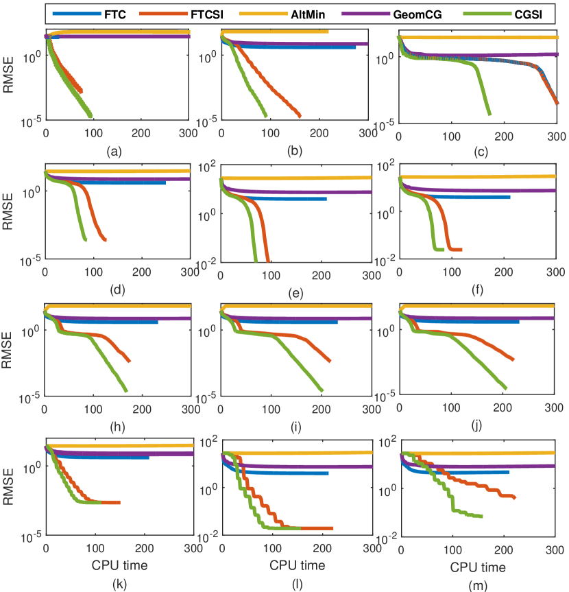
In the simulations, we complete a random tensor ${\mathbfcal{R}}$ whose size is fixed to $5000\times 5000\times 5000$ and multilinear rank to $(10,10,10)$. And it is generated by ${\mathbfcal{R}}={\mathbfcal{A}}\times_{1}\mathbf{B}_{1}\times_{2}\mathbf{B}_{2}\times_{3}\mathbf{B}_{3}$ where ${\mathbfcal{A}}\in\mathbb{R}^{10\times 10\times 10}$ and $\mathbf{B}_{i}\in\mathbb{R}^{5000\times 10}$ are random (multi-dimensional) arrays with i.i.d standard Gaussian entries. The side informations are encoded in three feature matrices. They are generated by $\mathbf{F}_{i}=\mathbf{B}_{i}+s\|\mathbf{B}_{i}\|_{F}\mathbf{N}_{i}$ where $\mathbf{N}_{i}$ is a noise matrix with entries drew from i.i.d normal distribution. The indices of the observed entries $\Omega$ are sampled from the full indices set of the $5000\times 5000\times 5000$ tensor uniformly at random. Its cardinality $|\Omega|$ is set to $OS\times D$ where $D=3\times(5000\times 10-10^{2})+10^{3}$ is the dimension of the manifolds of $5000\times 5000\times 5000$ tensors with multilinear rank $(10,10,10)$ and $OS$ is called the Over-Sampling ratio. We compare the five tensor completion solvers under the following four scenarios. In each run the compared solvers are started with the same initializer generated from random, and stopped when either the norm of the gradient is less than $10^{-4}$ or the number of iterations is more than 300. To show the effectiveness of the propose metric, we also implemented an Riemannian CG solver, with the least square metric Kasai and Mishra (2016). And the parameters of $CGSI$ and $FTCSI$ are set to the same values as they solve the same problem.

VII.3.1 Case 1: influence of sampling ratio

We study the number of observed samples on the performance of the compared solvers. We vary the oversampling ratio in the set $OS\in\{0.1,1,5\}$ while fixing the noise scale of the feature matrices to $10^{-5}$. Then, run the five solvers on each tasks. For each run, we set $\alpha_{i},1\leq i\leq 3$ are all set to $10/|\Omega|$ and $\lambda=0$ for CGSI and FTCSI. The parameters of other baselines are set to the defaults. We report the convergence behavior of the compared solvers in Fig. 5(a-c). Note that in Fig. 5(a) the RMSE curve of FTC coincides with that of GE and in Fig. 5(c) the RMSE curve of FTC coincides with that of FTCSI. From Fig. 5(a) and (b), we can see that only CGSI and FTCSI successfully bring the RMSE down below $10^{-2}$ when OS is smaller than $1$. This shows that when the observed entries are scarce, using the side information in the optimization can make a big difference on the accuracy of tensor completion task. And from Fig. 5(a-c), we can see that CGSI converges to the solution faster than FTCSI. This is shows that our proposed metric can indeed accelerate the convergence of Riemannian conjugate gradient descent method.

VII.3.2 Case 2: influence of noisy side information

To study the affect of noisy feature matrix on the performance of the proposed method. We fix the oversampling ratio to $OS=1$ and vary the noise scale of the feature $c$ matrix in the set $\{10^{-4},10^{-3},10^{-2}\}$. For CGSI and FTCSI, their parameters $\alpha_{i}$ are all set to $1$ and $\lambda$ is set to 00. The convergence behavior of the compared methods are reported in Fig. 5(d-f). From these figures we can see that when converging, the RMSE of CGSI and FTCSI are similar. This is because they solve the same problem. And even the feature matrices are noisy, the RMSE of CGSI and FTCSI are much better than the other baselines. These figures also show that CGSI is much faster than FTCSI, which is attributed to that CGSI is endowed with a better Riemannian metric.

VII.3.3 Case 3: influence of non-relevant features

We consider the performance of the proposed method, when the provided feature matrices $\mathbf{F}_{i}$ have much more columns than the correct ones $\mathbf{B}_{i}$. The matrices $\mathbf{F}_{i}\in\mathbb{R}^{5000\times 10(k+1)}$ is generated by augmenting the correct feature matrices $\mathbf{B}_{i}$ with $10k$ randomly generated columns. That is, we set $\mathbf{F}_{i}=[\mathbf{B}_{i},\mathbf{G}_{i}]+10^{-5}\|\mathbf{B}_{i}\|\mathbf{E}_{i}$ where $\mathbf{G}_{i}\in\mathbb{R}^{5000\times 10k}$ and $\mathbf{E}_{i}\in\mathbb{R}^{5000\times 10(k+1)}$ are random matrices with entries drew from i.i.d standard Gaussian distribution. We fix the oversampling ratio to $OS=1$, and vary the parameter $k\in\{10,30,50\}$. For CGSI and FTCSI, $\alpha_{i},1\leq i\leq 3$ are set to $0.5$ and $\lambda$ is set to 00. The parameters of other baselines are set to the default. We report the convergence behavior of the compared solvers in Fig. 5 (g-i). From these figures we can see that both CGSI and FTCSI successfully bring the RMSE down around $10^{-5}$ even when the columns of $\mathbf{F}_{i}$ are 50 times larger than $\mathbf{B}_{i}$. And These figures also shows that the proposed solver CGSI converges much faster than FTCSI, which is attributed to CGSI being endowed with a better Riemannian metric.

VII.3.4 Case 4: influence of noisy samples

We consider the case where the observed entries are noisy by adding a scaled Gaussian noise $\epsilon{\mathbf{\mathcal{P}}_{\Omega}}({\mathbfcal{E}})$ to ${\mathbf{\mathcal{P}}_{\Omega}}({\mathbfcal{R}})$ where ${\mathbfcal{E}}$ is a noise tensor with i.i.d standard Gaussian entries. We fix the oversampling ratio $OS$ to $1$, the noise scale $c$ of feature matrices to $10^{-4}$ and vary the noise scale of samples such that $\epsilon\in\{10^{-4},10^{-3},10^{-2}\}$. For CGSI and FTCSI, their parameters are set as follow. When $\alpha_{i}=5,1\leq i\leq 3$ and $\lambda=0$. The parameters of other baselines are set to defaults. We report the performance of the compared solvers in Fig. 5 (j-l). From these figures we can see that only the solvers for the proposed model, that is CGSI and FTCSI, bring the RMSE down to the level of noise $\epsilon$ when converging. This shows that when the observed entries are few, exploiting the side information can significantly improves the RMSE. Also we can see that CGSI converges much faster than FTCSI, this exhibit that the proposed metric (11) is able to accelerate the convergence of Riemannian conjugate gradient descent method.

Refer to caption
Figure 5: Simulation results of different solvers on the task of tensor completion.

References

  • Abraham et al. (2012) Ralph Abraham, Jerrold E Marsden, and Tudor Ratiu. Manifolds, tensor analysis, and applications, volume 75. Springer Science & Business Media, 2012.
  • Absil et al. (2009) P-A Absil, Robert Mahony, and Rodolphe Sepulchre. Optimization algorithms on matrix manifolds. Princeton University Press, 2009.
  • Acar et al. (2011) Evrim Acar, Tamara G. Kolda, and Daniel M. Dunlavy. All-at-once optimization for coupled matrix and tensor factorizations. In MLG’11, 2011.
  • Bell and Koren (2007) Robert M Bell and Yehuda Koren. Lessons from the netflix prize challenge. Acm Sigkdd Explorations Newsletter, 9(2):75–79, 2007.
  • Beutel et al. (2014) Alex Beutel, Partha Pratim Talukdar, Abhimanu Kumar, Christos Faloutsos, Evangelos E Papalexakis, and Eric P Xing. Flexifact: Scalable flexible factorization of coupled tensors on hadoop. In ICDM, pages 109–117. SIAM, 2014.
  • Chen et al. (2013) Shouyuan Chen, Michael R Lyu, Irwin King, and Zenglin Xu. Exact and stable recovery of pairwise interaction tensors. In NIPS, 2013.
  • Filipović and Jukić (2015) Marko Filipović and Ante Jukić. Tucker factorization with missing data with application to low-n-rank tensor completion. Multidimensional systems and signal processing, 26(3):677–692, 2015.
  • Foster et al. (2006) David H Foster, Kinjiro Amano, Sérgio MC Nascimento, and Michael J Foster. Frequency of metamerism in natural scenes. Journal of the Optical Society ofAmerica A, 23:2359–2372, 2006.
  • Golub and Van Loan (2012) Gene H Golub and Charles F Van Loan. Matrix computations, volume 3. JHU Press, 2012.
  • Jain and Oh (2014) Prateek Jain and Sewoong Oh. Provable tensor factorization with missing data. In Advances in Neural Information Processing Systems, pages 1431–1439, 2014.
  • Kasai and Mishra (2016) Hiroyuki Kasai and Bamdev Mishra. Low-rank tensor completion: a riemannian manifold preconditioning approach. In ICML, 2016.
  • Kolda and Bader (2009) Tamara G Kolda and Brett W Bader. Tensor decompositions and applications. SIAM review, 51(3):455–500, 2009.
  • Kressner et al. (2014) Daniel Kressner, Michael Steinlechner, and Bart Vandereycken. Low-rank tensor completion by riemannian optimization. BIT Numerical Mathematics, 54(2):447–468, 2014.
  • Liu et al. (2013) Ji Liu, Przemyslaw Musialski, Peter Wonka, and Jieping Ye. Tensor completion for estimating missing values in visual data. IEEE Transactions on Pattern Analysis and Machine Intelligence, 35(1):208–220, 2013.
  • Liu et al. (2015) Qiang Liu, Shu Wu, and Liang Wang. Cot: Contextual operating tensor for context-aware recommender systems. In AAAI, pages 203–209, 2015.
  • Liu et al. (2014) Yuanyuan Liu, Fanhua Shang, Hong Cheng, James Cheng, and Hanghang Tong. Factor matrix trace norm minimization for low-rank tensor completion. In Proceedings of the 2014 SIAM International Conference on Data Mining, pages 866–874. SIAM, 2014.
  • Liu et al. (2016) Yuanyuan Liu, Fanhua Shang, Wei Fan, James Cheng, and Hong Cheng. Generalized higher order orthogonal iteration for tensor learning and decomposition. IEEE transactions on neural networks and learning systems, 27(12):2551–2563, 2016.
  • Mishra (2014) Bamdev Mishra. A Riemannian approach to large-scale constrained least-squares with symmetries. PhD thesis, Universite de Liege, Liege, Belgique, 2014.
  • Mishra and Sepulchre (2014) Bamdev Mishra and Rodolphe Sepulchre. R3mc: A riemannian three-factor algorithm for low-rank matrix completion. In Decision and Control (CDC), 2014 IEEE 53rd Annual Conference on, pages 1137–1142. IEEE, 2014.
  • Mishra and Sepulchre (2016) Bamdev Mishra and Rodolphe Sepulchre. Riemannian preconditioning. SIAM Journal on Optimization, 26(1):635–660, 2016.
  • Narita et al. (2011) Atsuhiro Narita, Kohei Hayashi, Ryota Tomioka, and Hisashi Kashima. Tensor factorization using auxiliary information. In Joint European Conference on Machine Learning and Knowledge Discovery in Databases, pages 501–516. Springer, 2011.
  • Rai et al. (2015) Piyush Rai, Yingjian Wang, and Lawrence Carin. Leveraging features and networks for probabilistic tensor decomposition. In AAAI, pages 2942–2948, 2015.
  • Romera-Paredes and Pontil (2013) Bernardino Romera-Paredes and Massimiliano Pontil. A new convex relaxation for tensor completion. In Advances in Neural Information Processing Systems, pages 2967–2975, 2013.
  • Romera-Paredes et al. (2013) Bernardino Romera-Paredes, Hane Aung, Nadia Bianchi-Berthouze, and Massimiliano Pontil. Multilinear multitask learning. In Proceedings of the 30th International Conference on Machine Learning, pages 1444–1452, 2013.
  • Smith et al. (2016) Shaden Smith, Jongsoo Park, and George Karypis. An exploration of optimization algorithms for high performance tensor completion. In Proceedings of the 2016 ACM/IEEE conference on Supercomputing, 2016.
  • Wang et al. (2015) Yichen Wang, Robert Chen, Joydeep Ghosh, Joshua C Denny, Abel Kho, You Chen, Bradley A Malin, and Jimeng Sun. Rubik: Knowledge guided tensor factorization and completion for health data analytics. In Proceedings of the 21th ACM SIGKDD International Conference on Knowledge Discovery and Data Mining, pages 1265–1274. ACM, 2015.
  • Xu et al. (2015) Yangyang Xu, Ruru Hao, Wotao Yin, and Zhixun Su. Parallel matrix factorization for low-rank tensor completion. Inverse Problems & Imaging, 9(2), 2015.
  • Ye and Lim (2014) Ke Ye and Lek-Heng Lim. Distance between subspaces of different dimensions. arXiv preprint arXiv:1407.0900, 2014.
  • Yuan and Zhang (2015) Ming Yuan and Cun-Hui Zhang. On tensor completion via nuclear norm minimization. Foundations of Computational Mathematics, pages 1–38, 2015.
  • Zhang et al. (2014) Xiaoqin Zhang, Zhengyuan Zhou, Di Wang, and Yi Ma. Hybrid singular value thresholding for tensor completion. In AAAI, pages 1362–1368, 2014.
  • Zhang and Aeron (2016) Zemin Zhang and Shuchin Aeron. Exact tensor completion using t-svd. IEEE Transactions on Signal Processing, 2016.