A quark model study of strong decays of $X\left(3915\right)$

P. González Departamento de Física Teórica -IFIC
Universitat de Val ncia-CSIC
E-46100 Burjassot (Valencia), Spain.

(E-mail: pedro.gonzalez@uv.es)

Abstract

Strong decays of $X\left(3915\right)$ are analyzed from two quark model descriptions of $X\left(3915\right)$, a conventional one in terms of the Cornell potential and an unconventional one from a Generalized Screened potential. We conclude that the experimental suppression of the OZI allowed decay $X\left(3915\right)\rightarrow D\overline{D}$ might be explained in both cases as due to the momentum dependence of the decay amplitude. However, the experimental significance of the OZI forbidden decay $X\left(3915\right)\rightarrow\omega J/\psi$ could favor an unconventional description.
Keywords: quark, meson, potential

1 Introduction

In the last edition of the Review of Particle Physics [1] the former $X\left(3915\right)$ charmonium state has been assigned to a conventional $\chi_{c0}\left(3915\right)$ with quoted mass $M_{X(3915)}=3918.4\pm 1.9$ $MeV$ and total width $\Gamma_{X(3915)}=20\pm 5$ $MeV$. This assignment has been a matter of controversy: in references [2, 3] it has been argued that the mass, width, decay properties and production rates are incompatible with a $\chi_{c0}\left(2p\right)$ state expected from conventional descriptions as the ones provided by the Cornell model [4] or the Godfrey-Isgur model [5]. Indeed, alternative descriptions, based on four quark structures -meson-antimeson molecule, tetraquark, mixed charmonium-molecule…-, have been developed in the past (for an extensive review of these alternatives see the recent report [6] and references therein). In particular, some of the different molecular like treatments [7, 8, 9, 10] have allowed for the calculation of masses as well as strong and electromagnetic decay properties that can be compared to current data.

In this article we show that an unconventional description of the $X\left(3915\right),$ yet based on a quark-antiquark structure, as the one provided by the Generalized Screened Potential Model (GSPM) [11, 12], may give better account of its decay properties than the conventional one from the Cornell model. As a matter of fact the GSPM results, being closer to the ones obtained from molecular like treatments, may provide a reasonable description of data.

We shall centre first on the lack of evidence of the OZI allowed decay $X\left(3915\right)\rightarrow D\overline{D}$. By using two different decay models, ${}^{3}P_{0}$ and $C^{3\text{ }},$ for the calculation of the amplitude, we shall show that the observed experimental suppression may be explained either from the momentum dependence of the ${}^{3}P_{0}$ amplitude in the case of the GSPM description of $X\left(3915\right)$ or from the momentum dependence of the $C^{3\text{ }}$ amplitude in the case of the Cornell description of $X\left(3915\right)$. Therefore no definite conclusion about the conventional or unconventional nature of $X\left(3915\right)$ should be extracted from this decay. On the contrary, we shall show that the significant partial width for the OZI suppressed decay $X\left(3915\right)\rightarrow\omega J/\psi$, which we shall analyze later, might discriminate between both descriptions in favor of the GSPM one.

These contents are organized as follows. In Section 2 a comparative description of $X\left(3915\right)$ with the Cornell potential versus the Generalized Screened potential is presented. Then, in Section 3 a study of $X\left(3915\right)\rightarrow D\overline{D}$ with the ${}^{3}P_{0}$ and $C^{3}$ decay models is carried out for both descriptions of $X\left(3915\right)$, the results being compared to the ones obtained from other approaches. Section 4 is dedicated to the analysis of the decay $X\left(3915\right)\rightarrow\omega J/\psi$. Finally, in Section 5 our main results and conclusions are summarized.

2 $X\left(3915\right)$ quark model descriptions

The Cornell potential [4]

$$V_{Cor}(r)\equiv\sigma r-\frac{\zeta}{r}\text{ \ \ \ }\left(r:0\rightarrow\infty\right)$$ (1)

with the parameters $\sigma$ and $\zeta$ standing for the string tension and the color coulomb strength respectively, and refined models from it [5], have been very successful in the description of the heavy quarkonia spectra ($r$ standing for the quark-antiquark distance) below the open-flavor two meson thresholds. Above these thresholds the effect of two-meson channels have been explicitly implemented [13, 14] but a good overall description of data seems difficult to be attained.

In Table 1, from [12], the calculated masses for $J^{++}$ Cornell charmonium sates (fifth column) from $V_{Cor}(r)$, with standard effective parameters $\sigma=850$ MeV/fm, $\zeta=100$ MeV.fm , are listed (these values provide a reasonable overall spectral description of charmonium as well as bottomonium [11]). The value chosen for the charm mass $m_{c}=1348.6$ MeV will be justified below.

$J^{PC}$	$\begin{array}[c]{c}\text{GSPM}\\ \text{States}\end{array}$	$\begin{array}[c]{c}M_{GSPM}\\ \text{MeV}\end{array}$	$\begin{array}[c]{c}M_{PDG}\\ \text{MeV}\end{array}$	$\begin{array}[c]{c}M_{Cor}\\ \text{MeV}\end{array}$	$\begin{array}[c]{c}\text{Cornell}\\ \text{States}\end{array}$
$0^{++}$	$1p_{\left[T_{0},T_{1}\right]}$	$3456.1$	$3414.75\pm 0.31$	$3456.2$	$1p$
$1^{++}$	$1p_{\left[T_{0},T_{1}\right]}$	$3456.1$	$3510.66\pm 0.07$	$3456.2$	$1p$
$2^{++}$	$1p_{\left[T_{0},T_{1}\right]}$	$3456.1$	$3556.20\pm 0.09$	$3456.2$	$1p$
$1^{++}$	$2p_{\left[T_{0},T_{1}\right]}$	$3871.7$	$3871.69\pm 0.17$	$3910.9$	$2p$
$0^{++}$	$1p_{\left[T_{1},T_{2}\right]}$	$3897.9$	$3918.4\pm 1.9$	$3910.9$	$2p$
$2^{++}$	$2p_{\left[T_{0},T_{1}\right]}$	$3903.0$	$3927.2\pm 2.6$	$3910.9$	$2p$
$1^{++}$	$1p_{\left[T_{1},T_{2}\right]}$	$4017.3$
$0^{++}$	$1p_{\left[T_{3},T_{4}\right]}$	$4140.2$
			$X\left(4140\right)$
$2^{++}$	$1p_{\left[T_{1},T_{2}\right]}$	$4140.2$
$0^{++}$	$1p_{\left[T_{4},T_{5}\right]}$	$4325.1$	$X\left(4350\right)$	$4294.6$	$3p$

Table 1: Calculated $J^{++}$ charmonium masses, up to $4350$ MeV, from the Cornell potential $V_{Cor}:$ $M_{Cor},$ and from the Generalized Screened potential $V(r):M_{GSPM}$, with $\sigma=850$ MeV/fm, $\zeta=100$ MeV.fm and $m_{c}=1348.6$ MeV. For the GSPM the $0^{++}\left(1p_{\left[T_{2},T_{3}\right]}\right)$ row has been omitted since there is no bound state in that energy region; for $1^{++}$ we do not list any state above $4080$ MeV due to the current incomplete knowledge about thresholds above this energy; the same for $2^{++}$ states above $4224$ MeV. Masses for experimental resonances, $M_{PDG},$ have been taken from [1] (when a resonance appears in the Particle Listing section of [1] but not in the Summary Table we write the name of the resonance that contains the nominal mass between parenthesis). For $p$ waves we quote separately the $np_{0}$, $np_{1}$ and $np_{2}$ states.

We shall focus our attention on $X\left(3915\right)$, a $0^{+}(0^{++})$ charmonium state above the first corresponding $0(0^{++})$ threshold, $D\overline{D}$, at $3730$ MeV. In the Cornell model it should be assigned to the $2p$ state: $\chi_{c0}\left(2p\right)$. Although the calculated $\chi_{c0,1,2}\left(2p\right)$ mass in Table 1 ($3910.9$ MeV) is close to the experimental one ($3918.4$ MeV) a more stringent test of the model involving other observables should be done before making any definite assignment. For this purpose we shall consider strong decays for which there are some experimental information.

For the sake of comparison, an unconventional description from the so called Generalized Screened Potential Model (GSPM) will be used. The GSPM [11, 12] is based on an effective quark-antiquark static potential $V\left(r\right)$ that implicitly incorporates threshold effects, in particular color screening from meson-meson configurations. The model has been applied to heavy quarkonia showing that a reasonable overall description of $J^{++}$ resonances below and above thresholds and of $1^{--}$ resonances quite below threshold is feasible (the choice of the mass $m_{c}=1348.6$ MeV allows for a precise spectral description of $X(3872)$ as a $0\left(1^{++}\right)$ state). More precisely, $V\left(r\right)$ is obtained through a Born-Oppenheimer approximation from the lattice results for the energy of two static color sources (heavy quark and heavy antiquark) in terms of their distance, $E\left(r\right)$, when the mixing of the quenched quark-antiquark configuration with open flavor meson-meson ones is taken into account [15]. By calling $M_{T_{i}}$ with $i\geq 1$ the masses of the physical meson-meson thresholds, $T_{i}$, with a given set of quantum numbers $I(J^{PC})$, and defining $M_{T_{0}}\equiv 0$ for a unified notation (note that $T_{0}$ does not correspond to any physical meson-meson threshold), the form of $V\left(r\right)$ in the different energy regions (specified as energy interval subindices) reads:

$$V_{\left[M_{T_{0}},M_{T_{1}}\right]}(r)=\left\{\begin{array}[c]{c}\sigma r-\frac{\zeta}{r}\text{ \ \ \ \ \ \ \ \ \ \ \ \ \ \ \ \ \ \ \ \ \ \ }r\leq r_{T_{1}}\\ \\ M_{T_{1}}-m_{Q}-m_{\overline{Q}}\text{ \ \ \ \ \ \ \ \ \ }r\geq r_{T_{1}}\end{array}\right.$$ (2)

and

$$V_{\left[M_{T_{j-1}},M_{T_{j}}\right]}(r)=\left\{\begin{array}[c]{c}M_{T_{j-1}}-m_{Q}-m_{\overline{Q}}\text{ \ \ \ \ \ }r\leq r_{T_{j-1}}\\ \\ \sigma r-\frac{\zeta}{r}\text{\ \ \ \ \ \ \ \ \ \ \ }r_{T_{j-1}}\leq r\leq r_{T_{j}}\\ \\ M_{T_{j}}-m_{Q}-m_{\overline{Q}}\text{ \ \ \ \ \ \ \ \ \ }r\geq r_{T_{j}}\end{array}\right.$$ (3)

for $j>1,$ where $m_{Q}$ $\left(m_{\overline{Q}}\right)$ stands for the mass of the heavy quark (antiquark) and with the crossing radii $r_{T_{i}}$ $\left(i\geq 1\right)$ defined by the continuity of the potential as

$$\sigma r_{T_{i}}-\frac{\zeta}{r_{T_{i}}}=M_{T_{i}}-m_{Q}-m_{\overline{Q}}$$ (4)

Thus, $V\left(r\right)$ has in each energy region between neighbor thresholds a Cornell form but modulated at short and long distances by these thresholds. Thus, for example in Fig. 1 the form of $V\left(r\right)$ in the first and second energy regions is drawn for $c\overline{c}$ states with $I^{G}(J^{PC})=0^{+}(0^{++})$ quantum numbers, whose first threshold $T_{1}$ corresponds to $D^{0}\overline{D}^{0}$ and its second threshold $T_{2}$ to $D_{s}^{+}D_{s}^{-}$.

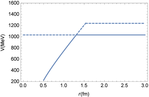
Figure 1: Generalized screened potential $V(r).$ The solid (dashed) line indicates the potential in the first (second) energy region for $0^{+}(0^{++})$ $c\overline{c}$ states with $m_{c}=1348.6$ MeV, $\sigma=850$ MeV/fm, $\zeta=100$ MeV.fm, $M_{T_{1}}=3730$ MeV ($r_{T_{1}}=1.31$ fm) and $M_{T_{2}}=3937$ MeV ($r_{T_{2}}=1.54$ fm).

From (2) it is clear that the description of states far below the lowest threshold $M_{T_{1}}$ is going to be identical to the Cornell one; however, a completely different description of the states above $M_{T_{1}}$ comes out. For instance, the $0^{+}(0^{++})$ bound state in the energy region $\left[M_{T_{1}=D^{0}\overline{D}^{0}},M_{T_{2}=D_{s}^{+}D_{s}^{-}}\right]$ is obtained by solving the Schrödinger equation for $V_{\left[M_{D^{0}\overline{D}^{0}},M_{D_{s}^{+}D_{s}^{-}}\right]}(r)$. This $1p_{\left[T_{1},T_{2}\right]}$ GSPM state with mass $3897.9$ MeV which should be assigned to $X(3915),$ see Table 1, differs greatly from the $2p$ Cornell one as can be checked in Fig. 2, from [12], where the respective radial wave functions are plotted.

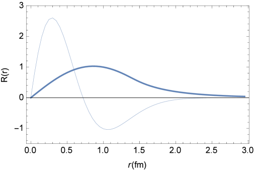
Figure 2: Radial wave functions R(r) (in units $fm^{-\frac{3}{2}}$) for the $0^{++}\left(1p_{\left[T_{1},T_{2}\right]}\right)$ GSPM state (thick line) and the $0^{++}\left(2p\right)$ Cornell state (thin line).

3 Decay models for $X\left(3915\right)\rightarrow D\overline{D}$

In order to get detailed predictions for the open flavor strong decay $X\left(3915\right)\rightarrow D\overline{D}$ we shall rely on a quark model framework. $X\left(3915\right)$ shall be considered as a $0^{+}\left(0^{++}\right)$ $c\overline{c}$ (Cornell or GSPM) state whose decay takes place through the formation of a light $q\overline{q}$ ($q=u,d$) pair that combines with $c\overline{c}$ giving rise to $D\overline{D}$. In the so called ${}^{3}P_{0}$ decay model [16] $q\overline{q}$ is created in the hadronic vacuum with $0^{++}$ quantum numbers. In the so called $C^{3}$ (Cornell Coupled-Channel) decay model [4] the $q\overline{q}$ creation is governed by the same potential generating the spectrum. Both models give a reasonable description of $I(J^{PC})$ charmonium decays [4, 17] below the corresponding first open flavor meson-meson thresholds.

For the ${}^{3}P_{0}$ as well as for the $C^{3}$ decay model the width for $X\left(3915\right)\rightarrow D\overline{D},$ in the rest frame of $X\left(3915\right),$ can be expressed as

$$\Gamma=2\pi\frac{E_{D}E_{\overline{D}}}{M_{X\left(3915\right)}}k_{D}\left|A\right|^{2}$$ (5)

where $E_{D}$ $\left(=E_{\overline{D}}\right)$ is the energy of the $D$ (or $\overline{D}$) meson given by

$$E_{D}=\sqrt{M_{D}^{2}+k_{D}^{2}}=E_{\overline{D}}$$ (6)

being $k_{D}$ the modulus of the three-momentum of $D$ (or $\overline{D}$) for which we shall use the relativistic expression

$$k_{D}=\frac{\sqrt{\left(M_{X}^{2}-4M_{D}^{2}\right)}}{2}$$ (7)

and $A$ stands for the decay amplitude.

In the ${}^{3}P_{0}$ model one has

$$\left|A\right|_{{}^{3}P_{0}}^{2}\equiv\gamma^{2}\left|M\right|^{2}$$ (8)

where the constant $\gamma$ specifies the strength of the pair creation, and the expression for $\left|M\right|^{2}$ can be derived from [17] in a straightforward manner (we use the same notation as in this reference) as

$$\left|M\right|^{2}=\frac{1}{32}I\left(-\right)^{2}$$ (9)

where

$$I\left(-\right)^{2}=\left|\begin{array}[c]{c}\frac{1}{\hbar^{\frac{9}{2}}}\int_{0}^{\infty}r_{X}^{2}dr_{X}\psi_{X}\left(r_{X}\right)\int p^{2}dp\widetilde{u}_{D}\left(p\right)\widetilde{u}_{\overline{D}}\left(p\right)\\ \left[-pj_{1}\left(\frac{pr_{X}}{\hbar}\right)j_{0}\left(\frac{m_{c}}{\left(m_{c}+m_{q}\right)}\frac{kr_{X}}{\hbar}\right)+\frac{m_{q}}{\left(m_{c}+m_{q}\right)}kj_{0}\left(\frac{pr_{X}}{\hbar}\right)j_{1}\left(\frac{m_{c}}{\left(m_{c}+m_{q}\right)}\frac{kr_{X}}{\hbar}\right)\right]\end{array}\right|^{2}$$ (10)

$m_{q}$ is the mass of the light quark, $\psi_{X}$ denotes the radial wave function of $X\left(3915\right)$ in configuration space and $\widetilde{u}_{D}\left(p\right)$ stands for radial wave function of $D$ in momentum space

$$\widetilde{u}_{D}\left(p\right)\equiv\sqrt{\frac{2}{\pi}}\int_{0}^{\infty}r_{D}^{2}dr_{D}\psi_{D}\left(r_{D}\right)j_{0}\left(\frac{pr_{D}}{\hbar}\right)$$ (11)

calculated from $\psi_{D},$ the radial wave function of $D$ in configuration space.

In order to simplify the calculation we shall approach as usual $\psi_{D}\left(r_{D}\right)$ by a gaussian (the same expression for $\psi_{\overline{D}}\left(r_{\overline{D}}\right)$)

$$\psi_{D}\left(r_{D}\right)=\frac{2}{\pi^{\frac{1}{4}}R_{D}^{\frac{3}{2}}}e^{-\frac{r_{D}^{2}}{2R_{D}^{2}}}$$ (12)

$R_{D}$ can be fixed either variationally or by requiring it to be equal to the root mean square (rms) radius, obtained from Cornell or the GSPM descriptions of $D$ (this implies the reset of the value of the coulomb strength $\zeta$ to get the spectral mass). By using the rms procedure we get $R_{D}=0.54$ fm. Then the use of the gaussian instead of the Cornell or the GSPM wave functions hardly makes any difference.

Notice that we have used $k$ in (10) for the three-momentum of $D$ (or $\overline{D}$) instead of the fixed $k_{D}.$ This will allow us to analyze the momentum dependence of the amplitude in order to have some idea of the possible effect of momentum dependent corrections. In this regard we should keep in mind that i) the strength of the pair creation may depend on momentum and ii) we calculate the amplitude from a non relativistic quark model.

The calculated ${}^{3}P_{0}$ widths for both descriptions, using $k=k_{D}$, are plotted in Table 2

	$\begin{array}[c]{c}X\left(3915\right)\\ 2p\text{ Cornell state}\end{array}$	$\begin{array}[c]{c}X\left(3915\right)\\ 1p_{\left[T_{1},T_{2}\right]}\text{ GSPMstate}\end{array}$
$\begin{array}[c]{c}{}^{3}P_{0}\\ \text{decay model}\end{array}$	$1.99\gamma^{2}$	$0.59\gamma^{2}$
$\begin{array}[c]{c}C^{3}\\ \text{decay model}\end{array}$	$33.66$	$1.95$

Table 2: Calculated widths in MeV for the decay $X\left(3915\right)\rightarrow D\overline{D}.$ The masses $M_{X\left(3915\right)}=3918$ MeV, $M_{D}=M_{\overline{D}}=1865$ MeV, from [1], have been used.

Usual values of $\gamma$, fitted from measured decays, are between $0.4$ and $7$. Therefore the calculated widths range from a few to dozens of MeV. This seems to be in contradiction with the observed experimental absence of the decay. Nonetheless, it is illustrative to examine the momentum dependence of the amplitude, plotted in Fig. 3.

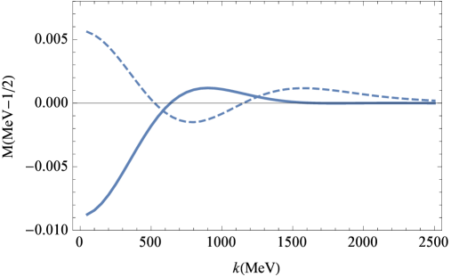
Figure 3: Momentum dependence of the ${}^{3}P_{0}$ decay ampitude for the GSPM (solid line) and Cornell (dashed line) descriptions of $X\left(3915\right).$

As can be checked, for the GSPM description the amplitude vanishes for a value of $k=637$ MeV close to $k_{D}=599.6$ MeV. Hence it is plausible that momentum dependent corrections to the ${}^{3}P_{0}$ decay model make the amplitude to vanish. Indeed, it has been shown that the use of harmonic wave functions for $X\left(3915\right)$ as well as for $D$ and $\overline{D}$ gives rise to a vanishing amplitude [18].

We may then tentatively conclude that the GSPM description combined with the ${}^{3}P_{0}$ decay model might provide an explanation to data.

It should be pointed out that alternative quark model calculations of the $X\left(3915\right)\rightarrow D\overline{D}$ decay from a ${}^{3}P_{0}$ decay model can be found in the literature. For example, in reference [19], with harmonic oscillator wave functions, the estimated width of the $0^{++}\left(2p\right)$ state, close to the total width of $X\left(3915\right)$ (a similar value was obtained in [20]), was used as an argument in favor of a conventional description. In reference [21], using a screened potential model description of $X\left(3915\right)$ [22], the calculated width was much larger than data disfavoring the $2p$ state assignment to $X\left(3915\right)$. A different result was found in reference [23], where the node structure in the Bethe Salpeter wave function employed gave rise to a small width. Finally, in reference [24], by using a gaussian expansion method in the framework of a chiral quark model to generate the wave functions, a width bigger than the total width of $X\left(3915\right)$ was found.

On the other hand, for the $C^{3}$ decay model one has

$$\left|A\right|_{Cor}^{2}\equiv\left|G\right|^{2}$$ (13)

The expression for $\left|G\right|^{2}$ has been derived from [4] by including the coulomb term of the potential as well as confinement. By using gaussians wave functions for $D$ and $\overline{D}$ as above and defining

$$\beta\equiv\frac{1}{2R_{D}^{2}}$$ (14)

the amplitude reads

$$\left|G\right|^{2}=g^{2}\left|\int_{0}^{\infty}dr_{X}\psi_{X}\left(r_{X}\right)e^{-\frac{\beta r_{X}^{2}}{2}}j_{0}\left(\frac{m_{c}}{\left(m_{c}+m_{q}\right)}\frac{kr_{X}}{\hbar}\right)J\left(r_{X}\right)\right|^{2}$$ (15)

where

$$g^{2}\equiv\left(\frac{2}{3\pi^{2}\hbar m_{q}^{2}\beta}\right)$$ (16)

and

$$J\left(r_{X}\right)\equiv\int_{a}^{b}dre^{-2\beta r^{2}}\left[2r_{X}\beta\left(\sigma r+\frac{\zeta}{r}\right)\left(e^{-2\beta rr_{X}}+e^{2\beta rr_{X}}\right)+\left(\sigma+\frac{\zeta}{r^{2}}\right)\left(e^{-2\beta rr_{X}}-e^{2\beta rr_{X}}\right)\right]$$ (17)

For the Cornell description of $X\left(3915\right)$ the integration limits are $a=0$ and $b=\infty$ whereas for the GSPM description one has $a=r_{T_{1}}=1.31$ fm and $b=r_{T_{2}}=1.54$ fm (notice that only for this interval the radial derivative of the Generalized Screened potential from which the amplitude is calculated [4] does not vanish).

The expression of the amplitude for the Cornell description is connected to the one given by equation (3.37) in [4], $I_{21}^{0},$ through

$$I_{21}^{0}=\beta\frac{\left(G\right)_{\zeta=0}}{g\sigma}$$ (18)

The calculated $C^{3}$ decay widths for both descriptions, using $k=k_{D}$, are plotted in Table 2. Again, the values obtained do not fit data. But if we plot the momentum dependence of the amplitude, Fig. 4, we realize that for the Cornell description the amplitude vanishes for a value of $k=558$ MeV close to $k_{D}=599.6$ MeV (this result differs slightly from the one obtained in reference [13] due to the differences in the expression of the amplitude).

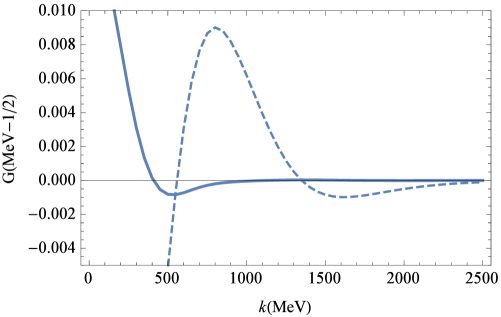
Figure 4: Momentum dependence of the $C^{3}$ decay ampitude for the GSPM (solid line) and Cornell (dashed line) descriptions of $X\left(3915\right).$

Hence it is plausible that momentum dependent corrections to the $C^{3}$ decay model make the amplitude to vanish. As a matter of fact, the use of $M_{X}=3910.9$ MeV, as given by the model, and $M_{D}=1869$ MeV as it corresponds to $D^{+}$ would give a vanishing amplitude for the non relativistic value of $K_{D}$.

We may then tentatively conclude that the Cornell description combined with the $C^{3}$ decay model might provide an explanation to data.

Putting together our tentative conclusions we may finally conclude that the observed suppression of the decay $X\left(3915\right)\rightarrow D\overline{D}$ might be equally well explained from a $C^{3}$ decay model with a Cornell description of $X\left(3915\right)$ and from a ${}^{3}P_{0}$ decay model with a GSPM description of $X\left(3915\right)$. Therefore, no conclusion about the conventional or unconventional nature of $X\left(3915\right)$ can be extracted from its decay to $D\overline{D}$.

Notice that the experimental suppression of the decay to $D\overline{D}$ may also be understood, at least qualitatively, from molecular like pictures. Thus, for instance, in reference [9] the dynamically generated $X\left(3915\right)$ (identifying $X(3915)$ with the so called $Y(3940)$ as done by the PDG) was dominantly a $D^{\ast}\overline{D}^{\ast}$ bound state decaying into pairs of light vectors or light vector-heavy vector mesons, whereas in reference [10] the $X\left(3915\right)$ was assumed to be a $D_{s}\overline{D}_{s}$ bound state so that its decay to $D\overline{D}$ is OZI suppressed.

4 The $X\left(3915\right)\rightarrow\omega J/\psi$ decay

Experimental information on this decay comes from the average of measured production rates in two-photon fusion [1]

$$\Gamma\left(X(3915)\rightarrow\gamma\gamma\right)\mathcal{B}\left(X(3915)\rightarrow J/\psi\omega\right)=54\pm 9\text{ eV}$$ (19)

and from the average of the product of branching fraction measurements for $X(3915)$ production in $B$ decay (see [3] and references therein)

$$\mathcal{B}\left(B^{+}\rightarrow K^{+}X(3915)\right)\mathcal{B}\left(X(3915)\rightarrow J/\psi\omega\right)=3.0_{-0.5-0.3}^{+0.6+0.5}\times 10^{-5}$$ (20)

In reference [3] it has been argued that if $X(3915)$ were a $\chi_{c0}\left(2p\right)$ Cornell state then it would be reasonable to assume that

$$\mathcal{B}\left(B^{+}\rightarrow K^{+}\chi_{c0}\left(2p\right)\right)\lesssim\mathcal{B}\left(B^{+}\rightarrow K^{+}\chi_{c0}\left(1p\right)\right)$$ (21)

The argument is based on the fact that the available phase space for $B^{+}\rightarrow K^{+}\chi_{c0}\left(2p\right)$ is significantly smaller than for $B^{+}\rightarrow K^{+}\chi_{c0}\left(1p\right)$ and on the assumption, based on reference [25], that $B$-meson decay rate to $\chi_{c0}\left(np\right)$ is proportional to $\left|R_{\chi_{c0}\left(np\right)}^{\prime}(0)\right|^{2}$ (we shall discuss this assumption for conventional Cornell states later on).

As the values of $\left|R_{0^{++}\left(2p\right)}^{{}^{\prime}}\left(0\right)\right|^{2}$ and $\left|R_{0^{++}\left(1p\right)}^{{}^{\prime}}\left(0\right)\right|^{2}$ do not differ much (see (24) below) one expects the ratio

$$\frac{\mathcal{B}\left(B^{+}\rightarrow K^{+}\chi_{c0}\left(2p\right)\right)}{\mathcal{B}\left(B^{+}\rightarrow K^{+}\chi_{c0}\left(1p\right)\right)}\lesssim 1$$ (22)

Then, using the experimental value $\mathcal{B}\left(B^{+}\rightarrow K^{+}\chi_{c0}\left(1p\right)\right)=1.5_{-0.14}^{+0.15}\times 10^{-4}$ one would get from (20)

$$\mathcal{B}\left(\chi_{c0}\left(2p\right)\rightarrow J/\psi\omega\right)>0.14$$ (23)

On the other hand $\Gamma\left(X(3915)\rightarrow\gamma\gamma\right)$ is known to be proportional to $\left|R_{X(3915)}^{\prime}(0)\right|^{2}$ [26]. Therefore, if $X(3915)$ were a $\chi_{c0}\left(2p\right)$ Cornell state we would expect the predicted ratio

$$\frac{\left(\Gamma\left(\chi_{c0}\left(2p\right)\rightarrow\gamma\gamma\right)\right)}{\left(\Gamma\left(\chi_{c0}\left(1P\right)\rightarrow\gamma\gamma\right)\right)}=\frac{\left|R_{0^{++}\left(2p\right)}^{{}^{\prime}}\left(0\right)\right|^{2}}{\left|R_{0^{++}\left(1p\right)}^{{}^{\prime}}\left(0\right)\right|^{2}}=1.4$$ (24)

to be a reasonable approximation to data. Then, using the experimental value

$$\Gamma\left(\chi_{c0}\left(1P\right)\rightarrow\gamma\gamma\right)=2.3\pm 0.4\text{ KeV}$$ (25)

one would get

$$\Gamma\left(\chi_{c0}\left(2p\right)\rightarrow\gamma\gamma\right)\sim 3.3\pm 0.6\text{ KeV}$$ (26)

However, the combination of (26) with (19) would give

$$\mathcal{B}\left(\chi_{c0}\left(2p\right)\rightarrow J/\psi\omega\right)\sim 0.017\pm 0.006$$ (27)

which is clearly incompatible with (23).

We may then tentatively conclude that the Cornell description of $X(3915)$ is not consistent with existing data for $\mathcal{B}\left(X(3915)\rightarrow J/\psi\omega\right).$

Let us now consider the GSPM description, say $X(3915)$ is a $1p_{\left[T_{1},T_{2}\right]}$ GSPM state. By using again the assumption $\mathcal{B}\left(B^{+}\rightarrow K^{+}\chi_{c0}\left(2p\right)\right)\lesssim\mathcal{B}\left(B^{+}\rightarrow K^{+}\chi_{c0}\left(1p\right)\right)$ an upper bound for $\mathcal{B}\left(B^{+}\rightarrow K^{+}X_{1p_{\left[T_{1},T_{2}\right]}}\right)$ can be found as follows. From [25] the decay rate of a $B^{+}$-meson to $0^{++}$ charmonium is given by the decay rate of the $\overline{b}$ antiquark with the light quark as a noninteracting spectator. To leading order in the QCD coupling the production rate, involving a color octet mechanism (a $c\overline{c}$ pair produced in a color octet $S$-wave), can be written as

$$\Gamma_{\left(\overline{b}\rightarrow 0^{++},\overline{s}\right)}=H_{8}^{\prime}\left(m_{b}\right)\Gamma_{8\left(\overline{b}\rightarrow c\overline{c}\left({}^{3}S_{1}\right),\overline{s}\right)}$$ (28)

where the subindex $8$ stands for color octet mechanism, $m_{b}$ is the mass of the $b$ quark and $H_{8}^{\prime}\left(m_{b}\right)$ is a nonperturbative parameter proportional to the probability for a $c\overline{c}$ pair produced in a color octet $S$-wave fragmenting into a color singlet $0^{++}$ bound state. This parameter can be expressed as

$$H_{8}^{\prime}\left(m_{b}\right)=a+eH_{1}$$ (29)

where$\ a$ is an unknown constant to be determined phenomenologically, $H_{1}$ is given by

$$H_{1}\approx\frac{1}{m_{c}^{4}}\left(\frac{9}{2\pi}\right)\left|R_{0^{++}}^{\prime}(0)\right|^{2}$$ (30)

with $m_{c}$ the mass of the $c$ quark and

$$e\equiv-\left(\frac{16}{27\beta}\right)\ln\left(\alpha_{s}\left(m_{b}\right)\right)$$ (31)

with $\beta=\frac{33-2n_{f}}{6}$ being $n_{f}$ the number of active quarks. Using $n_{f}=4$ and $\alpha_{s}\left(m_{b}\right)\approx 0.2$ [25] we get $e\approx 0.2$.

As the phase space is the same for the GSPM and the Cornell descriptions we get

$$\frac{\mathcal{B}\left(B^{+}\rightarrow K^{+}X_{1p_{\left[T_{1},T_{2}\right]}}\right)}{\mathcal{B}\left(B^{+}\rightarrow K^{+}\chi_{c0}\left(2p\right)\right)}=\frac{a+e\left(H_{1}\right)_{1p_{\left[T_{1},T_{2}\right]}}}{a+e\left(H_{1}\right)_{\chi_{c0}\left(2p\right)}}$$ (32)

By substituting the calculated values

$$\left|R_{0^{++}(1p_{\left[T_{1},T_{2}\right]})}^{{}^{\prime}}\left(0\right)\right|^{2}=3.57\text{ fm}^{-\frac{5}{2}}$$ (33)

$$\left|R_{0^{++}\left(2p\right)}^{{}^{\prime}}\left(0\right)\right|^{2}=272.25\text{ fm}^{-\frac{5}{2}}$$ (34)

we have

$$\frac{\mathcal{B}\left(B^{+}\rightarrow K^{+}X_{1p_{\left[T_{1},T_{2}\right]}}\right)}{\mathcal{B}\left(B^{+}\rightarrow K^{+}\chi_{c0}\left(2p\right)\right)}=\frac{a+0.1\text{ MeV}}{a+7.1\text{ MeV}}$$ (35)

Then using $\mathcal{B}\left(B^{+}\rightarrow K^{+}\chi_{c0}\left(2p\right)\right)\lesssim\mathcal{B}\left(B^{+}\rightarrow K^{+}\chi_{c0}\left(1p\right)\right)$ we obtain from (35) the bound

$$\mathcal{B}\left(B^{+}\rightarrow K^{+}X_{1p_{\left[T_{1},T_{2}\right]}}\right)\lesssim\left(\frac{a+0.1\text{ MeV}}{a+7.1\text{ MeV}}\right)\mathcal{B}\left(B^{+}\rightarrow K^{+}\chi_{c0}\left(1p\right)\right)$$ (36)

in terms of the unknown constant $a$.

Let us consider now $\Gamma\left(1p_{\left[T_{1},T_{2}\right]}\rightarrow\gamma\gamma\right).$ This width can be calculated from the predicted GSPM ratio ((notice that there is no difference between the Cornell $\chi_{c0}\left(1P\right)$ state and the $0^{++}\left(1p_{\left[T_{0},T_{1}\right]}\right)$ GSPM state)

$$\frac{\Gamma\left(1p_{\left[T_{1},T_{2}\right]}\rightarrow\gamma\gamma\right)}{\Gamma\left(\chi_{c0}\left(1P\right)\rightarrow\gamma\gamma\right)}=\frac{\left|R_{0^{++}\left(1p_{\left[T_{1},T_{2}\right]}\right)}^{{}^{\prime}}\left(0\right)\right|^{2}}{\left|R_{0^{++}\left(1p_{\left[T_{0},T_{1}\right]}\right)}^{{}^{\prime}}\left(0\right)\right|^{2}}=0.02$$ (37)

Using the experimental value $\Gamma\left(\chi_{c0}\left(1P\right)\rightarrow\gamma\gamma\right)=2.3\pm 0.4$ KeV one gets

$$\Gamma\left(0^{++}\left(1p_{\left[T_{1},T_{2}\right]}\right)\rightarrow\gamma\gamma\right)\simeq 0.02\left(\Gamma\left(\chi_{c0}\left(1p\right)\rightarrow\gamma\gamma\right)\right)_{Exp}=46\pm 8\text{ }eV$$ (38)

Therefore, if $X(3915)$ is a $1p_{\left[T_{1},T_{2}\right]}$ GSPM state, the combination of (38) with (19) gives

$$\mathcal{B}\left(1p_{\left[T_{1},T_{2}\right]}\rightarrow J/\psi\omega\right)>0.83$$ (39)

This implies from (20) that

$$\mathcal{B}\left(B^{+}\rightarrow K^{+}X_{1p_{\left[T_{1},T_{2}\right]}}\right)<3.6_{-0.6-0.4}^{+0.7+0.6}\times 10^{-5}$$ (40)

Hence making this bound equal to the one previously obtained (36), we get a phenomenological value for $a$ compatible with data. For the central experimental value $\mathcal{B}\left(B^{+}\rightarrow K^{+}X_{1p_{\left[T_{1},T_{2}\right]}}\right)<3.6\times 10^{-5}$ we have

$$a\sim 2.1\text{ MeV}$$ (41)

Hence a full consistent description of data is feasible. Furthermore, this value of $a$ gives a ratio

$$\frac{a+e\left(H_{1}\right)_{\chi_{c0}\left(2p\right)}}{a+e\left(H_{1}\right)_{\chi_{c0}\left(1p\right)}}\sim\frac{2.1+7.1}{2.1+5.0}=1.3$$ (42)

very close to the ratio

$$\frac{\left|R_{0^{++}\left(2p\right)}^{{}^{\prime}}\left(0\right)\right|^{2}}{\left|R_{0^{++}\left(1p\right)}^{{}^{\prime}}\left(0\right)\right|^{2}}=1.4$$ (43)

providing consistency to the argument used in [3].

We may then tentatively conclude that the GSPM description of $X(3915)$ might be consistent with existing data for $\mathcal{B}\left(X(3915)\rightarrow J/\psi\omega\right).$

Certainly one could argue that the calculated values of the square of the derivatives of the wave functions at the origin, on which our discussion is based, could vary when corrections to the Cornell and GSPM descriptions were considered. However, as we only deal with ratios involving such derivatives we do not expect significant changes from these corrections.

As the plausible account of data by the GSPM depends on the value of the unknown parameter $a$ some direct estimation of the $X(3915)\rightarrow J/\psi\omega$ decay width would be of great interest to confirm or refute our results. Unfortunately the QCDME (QCD Multipole Expansion) formalism developed to calculate hadronic decays [27, 28] is not very reliable when states above threshold are involved (see for example [29]). Nonetheless, if we assumed that corrections could be effectively incorporated by means of multiplicative factors then we might try to apply the QCDME to compare the decay widths obtained with the GSPM and Cornell descriptions. Even so, the calculation of these decay widths would be out of the scope of this article since it involves contributions from intermediate color octet states that should be consistently obtained with the model under consideration.

The only simple thing we can do is to use a scaling law as a very rough approach for the ratio of the decay widths being aware that the value obtained could differ even orders of magnitude from the real one (see [30] and references therein).

In the QCDME the $X(3915)\rightarrow J/\psi\omega$ decay corresponds to a three gluon E1-E1-E1 transition. As each E1 introduces a color-electric dipole moment that goes linearly with the $c\overline{c}$ distance $\overrightarrow{r}$ the scaling law reads

$$\frac{\Gamma\left(1p_{\left[T_{1},T_{2}\right]}\rightarrow J/\psi\omega\right)}{\Gamma\left(\chi_{c0}\left(2p\right)\rightarrow J/\psi\omega\right)}\simeq\left(\frac{\int drr^{2}R_{J/\psi}r^{3}R_{1p_{\left[T_{1},T_{2}\right]}}}{\int drr^{2}R_{J/\psi}r^{3}R_{\chi_{c0}\left(2p\right)}}\right)^{2}$$ (44)

where $R$ stands for the radial wave function.

By substituting the calculated integrals from the GSPM and the Cornell descriptions we get

$$\frac{\Gamma\left(1p_{\left[T_{1},T_{2}\right]}\rightarrow J/\psi\omega\right)}{\Gamma\left(\chi_{c0}\left(2p\right)\rightarrow J/\psi\omega\right)}\simeq 4$$ (45)

This value is about $13$ times smaller than the one obtained from (39) and (27), may be indicating the inadequacy of the scaling law and signaling the need for a more precise direct estimation of the $X(3915)\rightarrow J/\psi\omega$ decay before extracting any definite conclusion about the validity of the GSPM to describe the $X(3915).$

In this regard, it may be also illustrative to compare the result $\Gamma\left(X(3915)_{GSPM}\rightarrow\gamma\gamma\right)\simeq 46\pm 8$ eV, from which the bound $\mathcal{B}\left(X(3915)_{GSPM}\rightarrow J/\psi\omega\right)>0.83$ is obtained, with those obtained from molecular like model descriptions of $X(3915)$ (identifying $X(3915)$ with the so called $Y(3940)$ as done by the PDG). So, in reference [8], where the $X(3915)$ is considered as a $D^{\ast}\overline{D}^{\ast}$ hadronic molecule and a phenomenological lagrangian approach is followed, the values $\Gamma\left(X(3915)\rightarrow\gamma\gamma\right)\simeq 330$ eV and $\Gamma\left(X(3915)\rightarrow J/\psi\omega\right)\simeq 5.47$ MeV have been reported; these values are close to satisfy the experimental requirement (19). On the other hand, in reference [9] the calculated values $\Gamma\left(X(3915)\rightarrow\gamma\gamma\right)\simeq 31$ eV and $\Gamma\left(X(3915)\rightarrow J/\psi\omega\right)\simeq 1.52$ MeV are far from satisfying (19). Therefore, the GSPM result for $\Gamma\left(X(3915)\rightarrow\gamma\gamma\right)$ is closer to those obtained from molecular approaches than to the one resulting from the conventional Cornell description; with respect to the $X(3915)$ decay to $J/\psi\omega$ its GSPM value has to be, as shown above, significantly more dominant than in such approaches in order to reproduce current data.

5 Summary

A comparative study of the strong decays $X\left(3915\right)\rightarrow D\overline{D}$ and $X(3915)\rightarrow J/\psi\omega$ has been carried out from two quark model descriptions of $X\left(3915\right).$ The first description comes out from a Cornell potential that provides a reasonable fit to heavy quarkonia states lying below open flavor two meson thresholds; the second one is based on a Generalized Screened Potential Model (GSPM) that allows for a consistent heavy quarkonia description of $J^{++}$ states below and above thresholds and $1^{--}$ states quite below their corresponding threshold (in this last case there is no difference between the GSPM and Cornell potentials).

The $X\left(3915\right)\rightarrow D\overline{D}$ process has been studied from two decay models, the ${}^{3}P_{0}$ and the $C^{3}$ (Cornell Coupled-Channel), usually employed within the quark model framework. We have shown that the three-momentum of the final mesons ($D$ and $\overline{D}$) is close to the value that makes $i)$ the ${}^{3}P_{0}$ decay amplitude to vanish for a GSPM description of $X\left(3915\right)$ and $ii)$ the $C^{3}$ decay amplitude to vanish for a Cornell description of $X\left(3915\right).$ These results make plausible an explanation of the observed experimental absence of this decay through small momentum dependent corrections to the amplitudes. As a consequence, no discrimination between the two descriptions employed can be done from this decay.

A different situation may occur for $X(3915)\rightarrow J/\psi\omega.$ We have shown that an explanation of existing data involving the branching fraction $\mathcal{B}\left(X(3915)\rightarrow J/\psi\omega\right)$ seems to be impossible to attain from the Cornell description. On the contrary, the GSPM description might accommodate all the experimental information predicting a quite big branching ratio for this OZI non allowed decay. The experimental confirmation of this prediction would clearly point out to a non conventional nature of $X(3915)$ putting in question the $\chi_{c0}\left(2p\right)$ PDG assignment.

This work has been supported by Ministerio de Economía y Competitividad of Spain (MINECO) grant FPA2013-47443-C2-1-P, by SEV-2014-0398 and by PrometeoII/2014/066 from Generalitat Valenciana.

References

- [1] K. A. Olive et al. [Particle Data Group (PDG)], Chin. Phys. C 38, 090001 (2014).
- [2] F. K. Guo and U. G. Meissner, Phys. Rev. D 86, 091501 (2012).
- [3] S. L. Olsen, Phys. Rev. D 91, 057501 (2015).
- [4] E. Eichten, K. Gottfried, T. Kinoshita, K. D. Lane and T. M. Yan, Phys. Rev. D 17, 3090 (1978); Phys. Rev. D 21, 203 (1980).
- [5] S. Godfrey and N. Isgur, Phys. Rev. D 32, 189 (1985).
- [6] H-X. Chen, W. Chen, X. Liu and S-L. Zhu, Phys. Rep. 639, 1 (2016).
- [7] X. Liu and S-L. Zhu, Phys. Rev. D 80, 017502 (2009).
- [8] T. Branz, T. Gutsche and V. E. Lyubovitskij, Phys. Rev. D 80, 054019 (2009).
- [9] R. Molina and E. Oset, Phys. Rev. D 80, 114013 (2009); T. Branz, R. Molina and E. Oset, Phys. Rev. D 83, 114015 (2011).
- [10] X. Li and M. B. Voloshin, Phys. Rev. D 91, 114014 (2015).
- [11] P. González, J.Phys. G 41, 095001 (2014).
- [12] P. González, Phys. Rev. D 92, 014017 (2015).
- [13] E. Eichten, K. Lane and C. Quigg, Phys. Rev. D 69, 094019 (2004).
- [14] E. Eichten, K. Lane and C. Quigg, Phys. Rev. D 75, 014014 (2006).
- [15] G. S. Bali, H. Neff, T. Düssel, T. Lippert and K. Schilling (SESAM Collaboration), Phys. Rev. D 71, 114513 (2005).
- [16] A. Le Yaouanc, L. Oliver, O. Pène and J. C. Raynal in ”Hadron transitions in the quark model”, Gordon and Breach Science Publishers 1988; Phys. Rev. D 8, 2223 (1973).
- [17] S. Ono, Phys. Rev. D 23, 1118 (1981).
- [18] T. Barnes and S. Godfrey, Phys. Rev. D 69, 054008 (2004).
- [19] X. Liu, Z-G. Luo and Z-F. Sun, Phys. Rev. Lett. 104, 122001 (2010).
- [20] T. Barnes, S. Godfrey and E. S. Swanson, Phys. Rev. D 72, 054026 (2005).
- [21] Y-C. Yang, Z. Xia and J. Ping, Phys. Rev. D 81, 094003 (2010).
- [22] B-Q. Li and K-T. Chao, Phys. Rev. D 79, 094004 (2009).
- [23] Y. Jiang, G-L. Wang, T. Wang and W-L. Ju, Int. J. Mod. Phys. A 28, 1350145-1 (2013).
- [24] H. Wang, Y. Yang and J. Ping, Eur. Phys. J. A 50, 76 (2014).
- [25] G. T. Bodwin, E. Braaten, T. C. Yuan and G. P. Lepage, Phys. Rev. D 46, R3703 (1992).
- [26] W. Kuong, P. B. Mackenzie, R. Rosenfeld and J. L. Rosner, Phys. Rev. D 37, 3210 (1988).
- [27] K. Gottfried, Phys. Rev. Lett. 40, 598 (1978).
- [28] T.-M. Yan, Phys. Rev. D 22, 1652 (1980).
- [29] N. Brambilla et al., Eur. Phys. J. C71, 1534 (2011).
- [30] Y.-P. Kuang, Front. Phys. China 1, 19 (2006).