Measurement of Anticipative Power of a Retina by Predictive Information

Abstract

The predictive properties of a retina are studied by measuring the mutual information (MI) between its stimulation and the corresponding firing rates while it is being probed by a train of short pulses with stochastic intervals. Features of the measured MI at various time shifts between the stimulation and the response are used to characterize the predictive properties of the retina. By varying the statistical properties of the pulse train, our experiments show that a retina has the ability to predict future events of the stimulation if the information rate of the stimulation is low enough. Also, this predictive property of the retina occurs at a time scale similar to the well established anticipative phenomenon of omitted stimulus response in a retina. Furthermore, a retina can make use of its predictive ability to distinguish between time series created by an Ornstein–Uhlenbeck and a hidden Markovian process.

I Introduction

The ability to predict or anticipate future events is crucial for the survival of animals. Predicting dynamical inputs can compensate the latency during information transfer and provide predictive information for learning and behavior Berry and Schwartz (2011); Berry et al. (1999); Hosoya et al. (2005); Leonardo and Meister (2013); Bialek et al. (2001). In 2007, Schwartz Schwartz et al. (2007); Schwartz and Berry (2008) et al reported that there will be spontaneous responses from the ganglion cells in the retina of salamander and mice after a periodic light stimulation is abruptly stopped; with the latency of this spontaneous response being linearly related to the period of the stopped stimulation. In other words, the retina seems to anticipate when the next upcoming pulse should have occurred and produce a response if the upcoming pulse is missing. This timed response for the omitted pulse from the retina is known as omitted stimulus response (OSR). Phenomena similar to the OSR have also been reported for induced ocular motor behavior under periodic light stimuli in zebra fish larvae Sumbre et al. (2008) and growth of slime mold under periodic alternation of moisture or temperature Saigusa et al. (2008).

Ideally, one would like to quantify and model the predictive properties of a retina. Although the phenomenon of OSR has been discovered for more than 10 years, it is still not clear how to relate OSR to the predictive properties of the retina. In OSR, information of the stimulation is apparently coded into the timing of the pulses. However, when there are fluctuations in the inter-pulse intervals of the stimulation, it is difficult to identify or even produce OSR. Therefore, it is not feasible to make use of OSR in inferring the predictive properties of a retina for the general cases of a non-periodic stimulation which should contain much more information than a purely periodic one. Bialek and Tishby have introduced the idea of predictive information (PI) based on the statistical properties of the input and output signal of a data processing system Rubin et al. (2016); Bialek and Tishby (1999). Recently, this idea has been applied successfully to describe the response of a retina to a stimulation in the form of a stochastic moving bar by computing the mutual information, $I_{m}\left(\delta t\right)$, between the input and output as a function of time shift $\delta t$ between the two signals Palmer et al. (2015). Intuitively, the form of $I_{m}\left(\delta t\right)$ should be determined by the predictive dynamics of the retina. However, it is still not clear what kind of information one can extract from $I_{m}\left(\delta t\right)$.

In this work, we report our experimental results in quantifying the predictive properties of a retina by using the PI method mentioned above. With a retina plated on top of a multi-electrode array (MEA) probed by stochastic light pulses, $I_{m}\left(\delta t\right)$ is measured as a function of the properties of the light pulses; namely its mean inter-pulse interval ($\left\langle\tau\right\rangle$) and correlation time ($\tau_{cor}$). Our main finding is that the location of the peak of $I_{m}\left(\delta t\right)$ can be shifted from $-\delta t$ to $+\delta t$ by an increase of $\tau_{cor}$; suggesting that retina has the ability to predict (with some uncertainties) future events in the stimulation when the stimulation is regular enough. However, this ability of prediction can only be observed when $\left\langle\tau\right\rangle$ is in the range of 100 ms < $\left\langle\tau\right\rangle$ < 200 ms; similar to that of the OSR phenomenon mentioned above measured in bullfrog retinas. Furthermore, this predictive property of a retina can be used to distinguish the signals generated from an Ornstein–Uhlenbeck (OU) and an hidden Markovian (HMM) process; with the signal from the HMM process being identified as more predictable by the retina.

II Materials and Methods

Retinas used in the experiments are obtained under dim red light from bullfrogs which were dark adapted for 1 hour before dissection. Our sample is consisted of a piece of retina fixed on the 60-channel multi-electrode array (MEA, 200 µm inter-electrode distance with 10 µm electrode diameter) by a permeable membrane and perfused with oxygenated Ringer’s solution. Each retina preparation can last for 6-8 hours. Stimulations to the retina is in the form of a train of stochastic light pulses (pulse duration = 50 ms) generated from a LED (peak of wavelength = 560 nm, intensity = 5 cd/m²) which illuminates the whole retina through a projection lens. The interval between pulses is controlled by a computer to produce a train of pulses with different characteristics which will be described in details below. Responses from the retinas are recorded at 20 kHz through the local field potentials at the 60 electrodes of the MEA. Spike sorting is performed through the Offline Sorter software. Signals with ambiguous or multiple waveforms are discarded. Firing rates are calculated as the number of spikes identified within a 5 ms bin. Our experiments consist of recording responses of the retina for stimulations with different characteristics. The protocol is to present each set of stimuli continuously for 5 min in a random order, and the inter-experiment resting time is 2–3 min. For OSR measurements, the same stimuli constituted of 20 pulses are repeated for 10–20 trials with 3–5 sec inter-trial resting time. All the experiments are carried out in a dark room with temperature around 25 °C. In the results reported below, over ten retina samples are used and at least three retina samples (on average 10–20 waveforms sorted from each sample) were used to verify each experimental results.

III Results

Figure 1a shows inter-pulse-interval ($\tau$) of the stochastic pulse train used in the experiment as a function of time (with a discrete time step of 5 ms). The pulse train is characterized by three parameters; namely the mean inter-pulse interval ($\langle\tau\rangle$), the correlation time between inter-pulse intervals ($\tau_{cor}$) and the standard deviations of $\tau$. This stimulation series is generated by following the idea of Palmer et al Palmer et al. (2015) which is associated with a damped harmonic oscillator driven by noise, with the $i^{th}$ intervals being generated as:

$$\tau_{i+1} = \tau_{i}+v_{i}\Delta$$ (1)

$$v_{i+1} = \left(1-\Gamma\right)v_{i}-\omega^{2}\tau_{i}\Delta+\xi_{i}\sqrt{D\Delta}$$ (2)

where v is the rate of change of $\tau$, $\xi$ a Gaussian noise with zero mean with amplitude $D=1$. The iteration step size $\Delta$ is fixed at 1/60 in the iteration. Note that $\Gamma$/2$\omega$ is kept at 1.06 so that the system is slightly over-damped. To generate the stimulations, the series $\left\{\tau_{i}\right\}$ ($\equiv\left\{\tau_{1},\tau_{2},\ldots\right\}$) is first created by the iteration of Eq. (1) and Eq. (2). Then, the standard deviations of $\left\{\tau_{i}\right\}$ is rescaled to have a fixed value of 20 ms and an offset is added to $\left\{\tau_{i}\right\}$ to obtain the desired mean $\langle\tau\rangle$. With this method, the correlation of $\left\{\tau_{i}\right\}$ is not only controlled by $\Gamma$, the rescaling of its standard deviation and the addition of offset all affect the correlation time of the series. The correlation time of the resultant stimulation must then be measured by computing its autocorrelation function. Note that when $\tau_{cor}$ tends to $\infty$, we will recover the periodic stimulation in OSR. With this stochastic pulse train, we can stimulate the retina by temporal patterns with continuous adjustable $\langle\tau\rangle$ and $\tau_{cor}$. During each experiment reported below, such a pulse train is presented to the retina for 5 min. Figure 1b is the raster plot of the firings of the retina recorded by the MEA while Fig. 1c shows the average firing rate obtained from Fig. 1b.

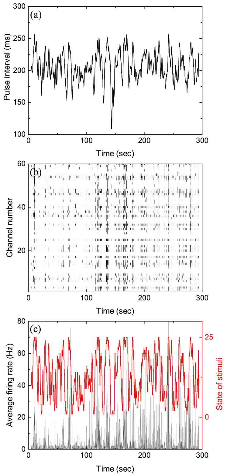
Figure 1: Stochastic pulse intervals and the induced retinal firing patterns. (a) Time series of pulse intervals generated by the iteration formula; $\langle\tau\rangle=200$ ms, $\sqrt{\langle(\tau-\langle\tau\rangle)^{2}\rangle}=20$ ms and $\tau_{cor}=4$ s. (b) Raster plot showing firing timestamps from 60 channels under the input shown in (a). (c) Average firing rate of the population recorded in (b). To calculate mutual information, the stimuli shown in (a) with varying pulse intervals are defined as equally distributed 25 states shown in red.

Mutual information at different time lag ($\delta t$) between the stimulation (Fig. 1a) and response (Fig. 1b) can then be calculated by using appropriate binning for the stimulation and response into discrete states. Figure 2 is the computed MI between stimulation and response from sorted firing waveforms in Fig. 1. The stimulation was binned into 25 equally distributed states ($S=\left\{s_{1},s_{2},\ldots,s_{25}\right\}$) while the number of spikes in one time window is used as the state index for the response ($R=\left\{r_{1},r_{2},\ldots\right\}$). The number of states for the response is then the maximum number of spikes for each channel within the time window. The maximal states within 50 ms is on average 10–15 spikes. The mutual information at time shift $\delta t$ is then given by:

$$I_{m}\left(S,R,\delta t\right)=\sum_{i}\sum_{j}p\left(s_{i},r_{j-k}\right)\log_{2}\frac{p\left(s_{i},r_{j-k}\right)}{p\left(s_{i}\right)p\left(r_{j-k}\right)}$$ (3)

where $p\left(x_{i}\right)$ is the probability of having a state $x_{i}$ and $p\left(s_{i},r_{j}\right)$ is the joint probability of the state $\left(s_{i},r_{j}\right)$. Note that the difference in state index $j-k$ denotes a shift in time of $\delta t$. It can be seen from Fig. 2a that the $I_{m}\left(S,R,\delta t\right)$ has a peak located at negative $\delta t$ and it is non-zero for $\delta t>0$. The location of the peak at negative $\delta t$ indicate that maximum information shared between $S$ and $R$ when $R$ is lagged behind $S$; confirming our intuition that the retina takes some time to reflect/process the information contained in $S$ in producing $R$.

Figure 2: An example of measured $I_{m}\left(\delta t\right)$ with stimulation shown in Fig. 1a. $I_{m}\left(\delta t\right)$ computed from shuffled data is also shown to serve as a base line. Three different $I_{m}\left(\delta t\right)$ obtained from three sorted signals in the same experiment are shown in the inset to demonstrate the variability of the data.

Similar to the finding of Palmer et al. (2015), the nonzero value of $I_{m}\left(S,R,\delta t\right)$ in Fig. 2a for $\delta t>0$ indicates that the firing patterns in retina provides predictive information for the future events in $S\left(t\right)$ from its history. In fact, $I_{m}\left(S,R,\delta t>0\right)$ is termed predictive information in Bialek and Tishby (1999). Also, it can be seen that $I_{m}\left(S,R,\delta t\right)$ can be nonzero extending into quite large $\delta t$; much longer than the correlation time of $S$. This last non-physical property of the measured $I_{m}$ originates from the fact we are computing $I_{m}$ from a finite time series. In order to find the baseline of our experimental $I_{m}$, either states of stimuli or firing patterns were randomly shuffled. The MI curve for shuffled data fluctuates at a nonzero and aligns with measurements at large $\delta t$, showing $I_{m_{0}}$ as a baseline due to finite data in Fig. 2b. Note that $I_{m_{0}}$ must be obtained for each firing patterns under different stimulations. $I_{m}$ reported below are all corrected as: $I_{m}^{*}=I_{m}-I_{m_{0}}$.

To visualize how much information is being shared between $S$ and $R$, Fig. 3 is a comparison of $I_{m}\left(S,S,\delta t\right)$, $I_{m}\left(R,R,\delta t\right)$ and $I_{m}\left(S,R,\delta t\right)$ from data displayed in Figs. 1 and 2. It can be seen that only a very small percentage of the information is being shared by $S$ and $R$. To quantify the amount of predictive information extracted by the retina, we have defined the predicting power based on measured $I_{m}$ as the ratio between the two areas in Fig. 3 as $P_{p}\left(S,R\right)=a/A$, where $A$ and $a$ are the area under the curves $I_{m}\left(S,S,\delta t\right)$ and $I_{m}\left(S,R,\delta t\right)$ at positive $\delta t$ respectively. This definition satisfies the intuitive notion that $P_{p}\left(S,S\right)$ or $P_{p}\left(R,R\right)$ equals to 1 and will allow the comparison of predictive information between different experiments. A remarkable feature of Fig. 3 is that while both $I_{m}\left(S,S,\delta t\right)$ and $I_{m}\left(R,R,\delta t\right)$ decay symmetrically about $\delta t=0$, $I_{m}\left(S,R,\delta t\right)$ seems to decay slower for $\delta t>0$. Since both $R$ and $S$ are symmetric with respect to time lag, the asymmetry of $I_{m}\left(S,R,\delta t\right)$ possibly comes from the anticipative nature of the retina dynamics in generating $R$.

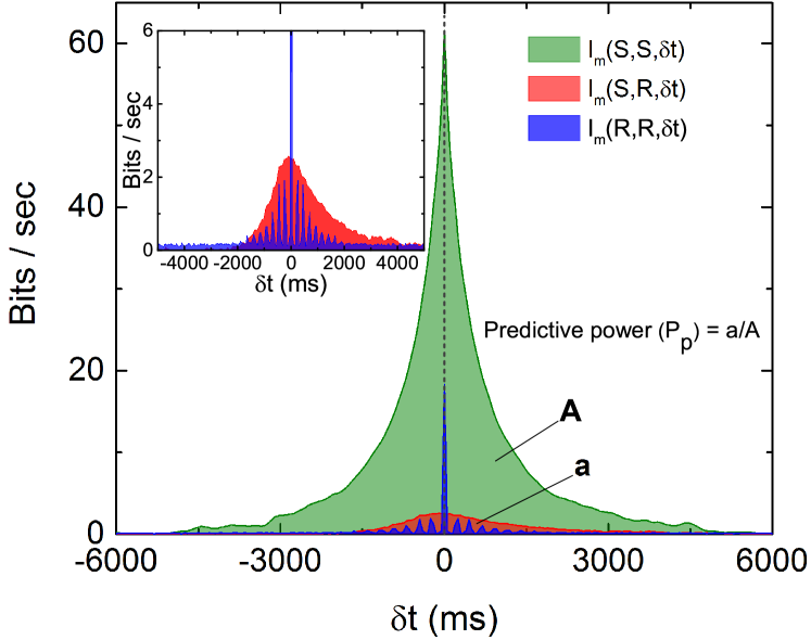
Figure 3: Comparison of the three $I_{m}\left(\delta t\right)$ as described in the text and the definition of predictive power ($P_{p}$). Note that both $I\left(S,S,\delta t\right)$ and $I\left(R,R,\delta t\right)$ are symmetric about their respective peaks but $I\left(S,R,\delta t\right)$ is not symmetric (inset). The oscillation observed in $I\left(R,R,\delta t\right)$ is caused by the quasi-periodicity of the stimulation light pulses.

To test the idea that asymmetry of $I_{m}\left(S,R,\delta t\right)$ is a manifestation of the predictive nature of the retina, two sets of $R$ are created artificially. First, the standard method to capture response of retina was applied, convolving the temporal spike trigger average (STA) obtained under random flicking stimuli with the stochastic pulse provided in experiment. The result fails to capture the asymmetry observed in experiment and over estimates the response delay. Alternatively, we have simulated a simple anticipative response from the stimulations $\left\{s_{i}\right\}$ as $\left\{r_{i}\right\}$ with $r_{i+1}=s_{i}+v_{i}\delta t$ where $v_{i}$ is the estimated “velocity” of the signal based on its $N$-step history $\left\{s_{i-N},s_{i-N+1},\ldots,s_{i}\right\}$. In other words, we are using linear extrapolation of $s_{i}$ to produce $r_{i+1}$. Figure 4 is the computed $I_{m}\left(\delta t\right)$ between the stimulations and their linear extrapolated responses together with the experimentally measured $I_{m}\left(\delta t\right)$. It can be seen that this simulated $I_{m}\left(\delta t\right)$ captures two essential features of the experimental measurements. First, the peak of the PI curve is not located at zero but at negative time lag. Second, the decay in $I_{m}\left(\delta t\right)$ is slower for $\delta t>0$. Obviously, the location of the peak of the $I_{m}\left(\delta t\right)$ curve in Fig. 4 is determined by the number of extrapolation. If we are extrapolating $n$-steps with $r_{i+n}=f\left(s_{i},s_{i-1},\ldots\right)$ for some function $f$, then the peak should be located at minus $n$ time lags.

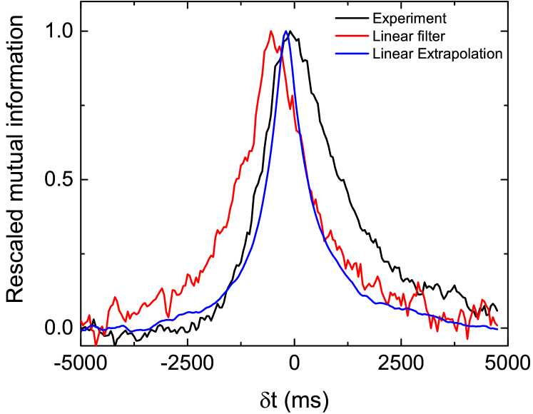
Figure 4: Comparison of $I_{m}\left(\delta t\right)$ with two simulated response. The experimental result (with parameters the same as those in Fig. 1) is shown in black. The red curve is obtained from the simulation convoluted with spike trigger average of the retina. The blue curve is simulated by linear extrapolation with a time window of 10 steps. These $I_{m}\left(\delta t\right)$s are normalized by their peak values for the ease of comparison. See text for details.

With the normalization introduced in Fig. 3, we can compare the predictive power ($P_{p}$) for stimulations with various $\langle\tau\rangle$ and $\tau_{cor}$. Figure 5 shows the measured dependence of $P_{p}$ on $\langle\tau\rangle$ and $\tau_{cor}$ by experiments similar to those shown in Fig. 3. Results shown in Fig. 5 are obtained from one single retina. The $P_{p}$ is measured for each channels of the MEA and error bars are obtained from the spread of these measured values. With fixed $\tau_{cor}=4$ s, it can be seen from Fig. 5a, $P_{p}$ falls off to a very small value around $\langle\tau\rangle=200$–$250$ ms. Note that a time scale of 200 ms is also the upper limit for a periodic stimulation to produce OSR in the bullfrog retina. Figure 5b shows $P_{p}$ under stimuli with different $\tau_{cor}$ when $\langle\tau\rangle$ fixed at $200$ ms. Note that the data is plotted in the inverse of $\tau_{cor}$. The idea is that the amount of information encoded into time series should increase with the inverse of its correlation time because an purely periodic signal (infinite correlation time) will not contain any information. With this interpretation, Fig. 5b indicates that the predictive power of the retina seems to be at its maximum when the information content of the stimulation is low and tends to its minimum when the information content is high. The characteristic time scale (halfway between the max and the min) determined from Fig. 5 is when $\tau_{cor}\approx 2.5$ s.

Figure 5: Predictive power ($P_{p}$) depends on the statistical properties of the simulation light pulses. (a) Measured $P_{p}$ at various $\langle\tau\rangle$ with $\tau$ being fixed to correlate in 20 steps for each value of $\langle\tau\rangle$. (b) Measured $P_{p}$ as a function of $1/\tau_{cor}$ with $\langle\tau\rangle$ fixed at 200 ms. The results are obtained from the same retina, and error bar indicates the deviation between 19 sorted signals.

One interesting feature of the measured $I_{m}$ during our scan of $\tau_{cor}$ at fixed $\langle\tau\rangle$ is that the peak location of the $I_{m}$ shifted from negative $\delta t$ to positive $\delta t$ as $\tau_{cor}$ is increased. Figure 6 shows the dependence of $\delta t_{p}$ as a function of $\tau_{cor}^{-1}$ where $\delta t_{p}$ is the distance of the peak location of $I_{m}$ from the line of $\delta t=0$. The inset of Fig. 6 shows the definition of peak location ($\delta t_{p}$) and the forms of $I_{m}\left(\delta t\right)$ for $\tau_{cor}=0.2$, $4.0$, and $7.0$ s. At first sight, one might expect $\delta t_{p}$ to be always negative because it will always take time for stimulations just to propagate through the different layers and synapses of the retina. That will be true if the retina is just a passive filter. The fact that $\delta t_{p}$ can be shifted to positive indicates that the retina is actively predicting the future events of the stimulations. This interpretation is consistent with the result of Fig. 5b which suggests that prediction is possible only when the input signal is regular enough.

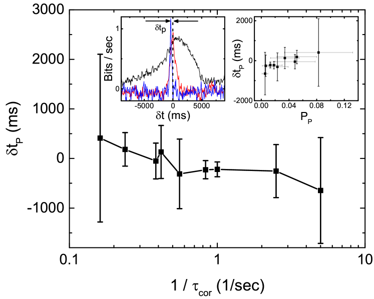
Figure 6: Latency to peak ($\delta t_{p}$) of $I_{m}\left(\delta t\right)$ as a function of $\tau_{cor}$ obtained from 19 sorted signals in the same retina. The left inset shows the definition of $\delta t_{p}$ and the measured $I_{m}\left(\delta t\right)$ with $\tau_{cor}$ = 0.2 (blue), 4 (red), 7 s (black). Right inset shows the relation between $\delta t_{p}$ and $P_{p}$ calculated from the same data

IV Discussions

Although the periodic input used in OSR and the stochastic pulses used in this study seem to be quite different, the periodic pulses are in fact a limiting case of the stochastic pulses when the correlation time of the inter-pulse interval becomes infinite. With this consideration, one can think of the periodic pulses used in the phenomenon of OSR as the carrier of information very much like the carrier wave in an FM radio signal and the information is being encoded into the deviations (fluctuations) from the carrier period. Therefore, the stochastic pulses (with a fixed mean period) used in our experiments are then encoding information in its deviations from the mean. The amount of information encoded can then be characterized by the correlation time; the longer the $\tau_{cor}$, the less the amount of encoded information. With a periodic stimulation (infinite correlation time), there is no information encoded. In fact, this carrier wave picture is supported by our finding that both OSR and $\langle\tau\rangle$ for optimal prediction have the same time scale.

We have therefore extended the study of anticipative capability of a retina from probing it with period stimulations to stochastic stimulations. Although the responses of the retina induced by these two types of stimulations seem to be very different, they are of the same nature. In the OSR, a clear transient, spontaneous (anticipative) response can be observed in the phenomenon of OSR after the termination of the periodic stimulations while there seems to be no clear anticipative responses can be identified after the termination of the stochastic stimulations. However, the results shown in Fig. 6 show that the retina is generating signals ahead of the stimulation with similar information. That is: the retina is actively producing spontaneous output corresponding to future events of the stimulation; similar to the case of OSR.

The picture emerges from the above discussions is that the retina is spontaneously/actively producing output to predict the future. The location of $\delta t_{p}$ can then be used as an indicator of the complexity or predictability of the stimulation. Intuitively, $\delta t_{p}$ will be more negative when the signals is more complex or more difficult to predict.

To test this idea, we have also performed experiments with stimulations generated by an OU process. We have tuned the OU process in such that its time scales and fluctuations are similar to those used in our experiments reported above. Figure 7 is a comparison for $I_{m}$ obtained from the OU process and that from Fig. 3. It can be seen that the peak of $I_{m}$ from the OU process lags behind from that of our experiment; demonstrating that retina can distinguish these two types of signals and indicate that the time series from the OU process is more complex that that used in our experiment. Note that the OU process is a Markovian process while the time interval signal used in our experiment is not. There is a hidden variable $v$, which can be deduced from successive values of pulse interval, forming a hidden Markov Model. Our experimental results show that the retina somehow manages to make use of this hidden information to anticipate the next time interval and therefore produce a peak in $I_{m}$ which can be located at $\delta t_{p}>0$. It is well known that neural field models for a retina can successfully produce the anticipative tracking of a moving object spatially. It is still not known how a retina can do the same in the time domain Yang et al. (2015).

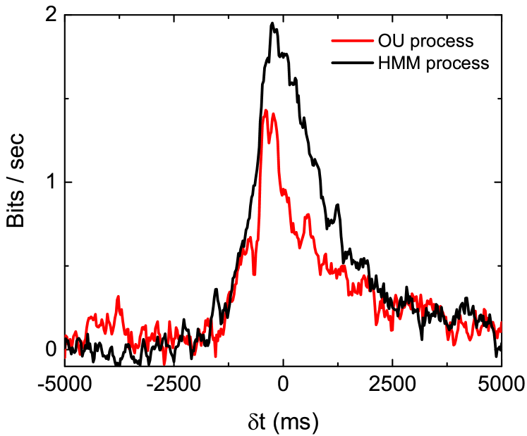
Figure 7: Discriminating OU and the HMM process by a retina. Measured $I_{m}\left(\delta t\right)$ with stimulations generated from an OU process (red) and that similar to Fig. 1a (black); with $\langle\tau\rangle=200$ ms and $\tau_{cor}=4$ s for both stimulations.

References

- Berry and Schwartz (2011) Michael J. II Berry and Gregory Schwartz, “Retina as Embodying Predictions about the Visual World,” in Predictions in the Brain: Using Our Past to Generate a Future (Oxford University Press, 2011) pp. 295–310.
- Berry et al. (1999) Michael J. Berry, Iman H. Brivanlou, Thomas A. Jordan, and Markus Meister, “Anticipation of moving stimuli by the retina,” Nature 398, 334–338 (1999).
- Hosoya et al. (2005) Toshihiko Hosoya, Stephen A. Baccus, and Markus Meister, “Dynamic predictive coding by the retina,” Nature 436, 71–77 (2005).
- Leonardo and Meister (2013) Anthony Leonardo and Markus Meister, “Nonlinear Dynamics Support a Linear Population Code in a Retinal Target-Tracking Circuit,” Journal of Neuroscience 33, 16971–16982 (2013).
- Bialek et al. (2001) W. Bialek, I. Nemenman, and N. Tishby, “Predictability, Complexity, and Learning,” Neural Computation 13, 2409–2463 (2001).
- Schwartz et al. (2007) Greg Schwartz, Rob Harris, David Shrom, and Michael J. Berry, “Detection and prediction of periodic patterns by the retina,” Nature Neuroscience 10, 552–554 (2007).
- Schwartz and Berry (2008) G. Schwartz and M. J. 2nd Berry, “Sophisticated Temporal Pattern Recognition in Retinal Ganglion Cells,” Journal of Neurophysiology 99, 1787–1798 (2008).
- Sumbre et al. (2008) Germán Sumbre, Akira Muto, Herwig Baier, and Mu-Ming Poo, “Entrained rhythmic activities of neuronal ensembles as perceptual memory of time interval,” Nature 456, 102–106 (2008).
- Saigusa et al. (2008) Tetsu Saigusa, Atsushi Tero, Toshiyuki Nakagaki, and Yoshiki Kuramoto, “Amoebae Anticipate Periodic Events,” Physical Review Letters 100, 018101 (2008).
- Rubin et al. (2016) Jonathan Rubin, Nachum Ulanovsky, Israel Nelken, and Naftali Tishby, “The Representation of Prediction Error in Auditory Cortex,” PLOS Comput Biol 12, e1005058 (2016).
- Bialek and Tishby (1999) William Bialek and Naftali Tishby, “Predictive Information,” (1999), arXiv:cond-mat/9902341 .
- Palmer et al. (2015) Stephanie E. Palmer, Olivier Marre, Michael J. Berry, and William Bialek, “Predictive information in a sensory population,” Proceedings of the National Academy of Sciences 112, 6908–6913 (2015).
- Yang et al. (2015) Ying-Jen Yang, Chun-Chung Chen, Pik-Yin Lai, and C. K. Chan, “Adaptive synchronization and anticipatory dynamical systems,” Physical Review E 92, 030701 (2015).